55 Cancri (Copernicus): A Multi-Planet System with a Hot Super-Earth and a Jupiter Analogue

Abstract

The star 55 Cancri was one of the first known exoplanet hosts and each of the planets in this system is remarkable. Planets b and c are in a near 1:3 resonance. Planet d has a 14.5 year orbit, and is one of the longest known orbital periods for a gas giant planet. Planet e has a mass of 8 $M_{\oplus}$ and transits this bright star, providing a unique case for modeling of the interior structure and atmospheric composition of an exoplanet. Planet f resides in the habitable zone of the star. If the planets are approximately co-planar, then by virtue of having one transiting planet, this is a system where the Doppler technique has essentially measured the true mass of the planets, rather than just $M\sin i$. The unfolding history of planet discovery for this system provides a good example of the challenges and importance of understanding the star to understand the planets.

1 Introduction

Transiting exoplanets with well-determined masses offer a unique opportunity for understanding the interior structure, chemical composition, evolution and atmospheric properties of exoplanets. The brightest known transit host star is 55 Cancri (55 Cnc), with a $8M_{\oplus}$ mass transiting planet in a 0.7356 day orbit (Winn et al. 2011; Demory et al. 2011). This star also has 4 other known exoplanets. The gas giant planet 55 Cnc b (Butler et al. 1997) was the fourth exoplanet discovered with the Doppler technique. Five years later, two more planets, 55 Cnc c and d, were announced in the system (Marcy et al. 2002). 55 Cnc d was remarkable in being the first planet known to orbit beyond 4AU. McArthur et al. (2004) announced the discovery of, 55 Cnc e. It was later learned that this orbital period was an alias of the true period, which is a remarkable 0.7365 days (18 hours). This revision distinguished 55 Cnc e as having the shortest known orbital period at that time. Fischer et al. (2008) added the last known planet to this system, 55 Cnc f, which orbits in the habitable zone.

Over the decade of exoplanet discoveries in the 55 Cnc system, several things went wrong that led to transient periods of confusion and misinterpretations. An incorrect infrared excess was measured, leading to the false interpretation of a significant debris disk. The modeling of an orbital period for 55 Cnc e was a case study of aliases in time series data; that period was revised from 2.8 d (McArthur et al. 2004) to 0.74 d (Dawson & Fabrycky 2010). Before the revision to this orbital period for 55 Cnc e, photometric surveys that targeted the incorrect transit ephemeris naturally missed what eventually turned out to be one of the most scientifically valuable transiting planets. The carbon abundance in the host star was intially overestimated, leading to confusion in the interpretation of the interior structure of 55 Cnc e. Ultimately, the story of 55 Cnc demonstrates the importance of understanding the host star to understand the orbiting planets.

2 The Host Star

Understanding the host star is important for understanding the nature (mass, radius, orbital evolution) of prospective planets. 55 Cancri (also known as 55 Cnc, $\rho^{1}$ Cancri, HD 75732, HIP 43587, HR 3522) is a bright G8V star, just 41 parsecs away. It is the primary component of a visual binary system. The secondary component, $\rho^{1}{\rm Cnc\,B}$, is about 7 magnitudes fainter ($V\sim 13$) with an angular separation of $\sim 85"$, corresponding to a projected physical separation of 1100 AU. The absolute radial velocities for the primary and secondary star are $27.3\pm 0.3$ and $27.4\pm 0.3$ km s^-1 respectively (Nidever et al. 2002), providing strong support for a gravitationally bound wide binary system.

2.1 The Confusing Question of a Debris Disk

One early controversy over 55 Cnc centered on whether or not the star had a reprocessing disk. Dominik et al. (1998) suggested that 55 Cnc had a Vega-like dust disk based on Infrared Space Observatory (ISO) data and Trilling & Brown (1998) claimed that they had resolved the disk out to $3.^{\prime\prime}2$ with near infrared coronographic images. However, Jayawardhana et al. (2000) was not able to confirm this result; they found the sub-mm emission to be a factor of 100 lower than expected for the reported disk. Schneider et al. (2001) imposed an upper limit on the NIR flux with NICMOS on HST that was 10 times lower than that reported by Trilling & Brown (1998). Jayawardhana et al. (2002) found 3 faint background sub-mm sources and it is possible that the faint binary companion may have contributed to the early source confusion. The best current assessment is that a reprocessing disk has not yet been detected around 55 Cnc.

2.2 Piecing Together the Fundamental Parameters

Ford et al. (1999) list a sampling of published effective temperatures for 55 Cnc that range from 4460 to 5336 K and discuss their inability to find a self-consistent stellar evolutionary model, given the poor quality of the observed parameters. Even the question of whether 55 Cnc was a main sequence star or a subgiant was disputed. While 55 Cnc is a few tenths of a magnitude brighter than the zero age main sequence, this is likely because of high metallicity, which was first noted by Greenstein & Oinas (1968).

Although stellar ages are notoriously difficult to determine (Mamajek & Hillenbrand 2008), model isochrones can be used to estimate an age for 55 Cnc. Published photometry was fitted with a spectral energy distribution by von Braun et al. (2011) to derive a bolometric luminosity. Using their interferometrically measured stellar radius $0.943\pm 0.01$ to derive $T_{\rm eff}~{}$ = $5196\pm 24{\rm K}$, the authors adopted the ${\rm[Fe/H]}$ published by Valenti & Fischer (2005) to fit Yonsei-Yale isochrones (Demarque et al. 2004; Kim et al. 2002; Yi et al. 2004), yielding a stellar mass of $0.905\pm 0.015M_{\odot}$ and an age of $10.2\pm 2.2$ Gyr. This age was initially at odds with the statistical kinematic age of 1 Gyr suggested by Eggen (1995); however the kinematic age was later revised by Reid (2002) who find the space motion velocity relative to the LSR to be 29.5 km s^-1, similar to disk stars with ages between $2-8$ Gyr. Gonzalez & Vanture (1998), and Brewer et al. (2016) both carried out fine spectroscopic modeling to determine stellar temperature and abundances and then used isochrone fitting to estimate the stellar age of 7.9 Gyr for 55 Cnc.

The age, rotation rate, magnetic field strength and chromospheric activity of stars are all physically correlated and therefore can be used to collectively piece together a self-consistent characterization of a star. As magnetic field lines emerge from the surfaces of stars, they suppress local convection and produce cooler regions, or starspots, in the photosphere. Photometric rotation periods can be measured for younger stars with larger spots (from stronger magnetic fields) using ground-based time series photometry. Marcy et al. (2002) obtained ground-based photometry for 55 Cnc that was constant at the level of 0.0012 magnitudes without any indication of rotational variability, consistent with a slowly rotating star with small spots.

Chromospheric activity measurements offer the best way for estimating the rotational periods of slowly rotating stars like 55 Cnc. Magnetic fields transport energy into the lower chromosphere and produce emission in deep spectral line cores such as the calcium II H (396.9 nm) and K (393.4 nm), calcium infrared triplet (849.8, 845.2, 866.2 nm), and the hydrogen Balmer lines (486.1 and 656.3 nm). The correlation between chromospheric activity and the rotation period of stars was first noted by Kraft (1967). The 30-year Mount Wilson Observatory HK Project (Wilson 1978; Vaughan et al. 1978; Duncan et al. 1991; Baliunas et al. 1995) measured Ca II H&K emission to study stellar chromospheric activity and variability in bright stars. The consistency and duration of this data set make it a touchstone for all studies of chromospheric activity.

Ca II H&K emission is parameterized by $S_{HK}$, a measure of flux in the line core relative to flux in adjacent continuum bands. Since late type stars have much weaker near-UV continuum than earlier type stars, $S_{HK}$ values cannot be directly compared for stars with different spectral types. Instead, $S_{HK}$ can be transformed to $\log R^{\prime}_{HK}$, the fraction of a star’s bolometric luminosity from the lower chromosphere after accounting for photospheric contributions (Noyes et al. 1984b; Soderblom 1985; Mamajek & Hillenbrand 2008). The Noyes et al. (1984b) calibration between Ca II H&K emission and rotation periods for stars with a range of $B-V$ color from 0.4 to 1.4 provides a good way to estimate rotation periods, even for older and more slowly rotating stars. Henry et al. (2000) report an average $S_{HK}=0.19$ and $\log R^{\prime}_{HK}=-4.949$ over 6 yr of monitoring 55 Cnc, implying a rotation period, ${\rm P_{rot}}=42.2$d, consistent with other activity-based estimates of 42 to 44 days (Soderblom 1985; Baliunas et al. 1997; Bell & Branch 1976). Isaacson & Fischer (2010) measure a slightly lower activity level, $\log R^{\prime}_{HK}$ = -4.991, implying a rotational period of about 47 days.

Parameter	Value	Source
Spectral Type	G8V	Perryman et al. (1997, Hipparcos)
V Magnitude	6.1	Perryman et al. (1997, Hipparcos)
Parallax	$81.03\pm 0.75\,{\rm mas}$	Perryman et al. (1997, Hipparcos)
${\rm M_{V}}$	5.64	(using Hipparcos photometry and parallax)
Radial Velocity	$27.3\pm 0.3$	Nidever et al. (2002)
Mass	0.71	Brewer et al. (2016)
Radius (aiso)	0.93	Ford et al. (1999)
Radius (aiso)	0.92	Brewer et al. (2016)
Radius (aintrfmtry)	$0.943\pm 0.01$	von Braun et al. (2011)
Luminosity	0.59 $L_{\odot}$	Brewer et al. (2016)
${\rm B-V}$	0.869	Perryman et al. (1997, Hipparcos)
${\rm T_{eff}}$ (aintrfmtry)	$0.943\pm 0.01$	von Braun et al. (2011)
${\rm T_{eff}}$ (aspectr)	5250 K	Brewer et al. (2016)
$\log g$ (aiso)	4.5	Ford et al. (1999)
$\log g$ (aspectr)	4.36	Brewer et al. (2016)
${\rm[M/H]}$	0.34	Brewer et al. (2016)
${\rm[Fe/H]}$	0.35	Brewer et al. (2016)
${\rm[Mg/H]}$	0.32	Brewer et al. (2016)
${\rm[Si/H]}$	0.33	Brewer et al. (2016)
${\rm[O/H]}$	0.32	Brewer et al. (2016)
Mg/Si	0.87	Delgado Mena et al. (2010)
Mg/Si	0.984	Brewer & Fischer (2016)
Si/Fe	1.098	Brewer et al. (2016)
${\rm C/O}$	1.12	Delgado Mena et al. (2010)
${\rm C/O}$	$0.534\pm 0.06$	Brewer & Fischer (2016)
${\rm P_{rot}}$ ($S_{HK}$)	42.2d	Henry et al. (2000)
${\rm P_{rot}}$ ($S_{HK}$)	42.2d	Isaacson & Fischer (2010)
$S_{HK}$	0.19	Henry et al. (2000)
$S_{HK}$	0.18	Isaacson & Fischer (2010)
$\log R^{\prime}_{HK}$	-4.949	Henry et al. (2000)
$\log R^{\prime}_{HK}$	-4.991	Isaacson & Fischer (2010)
Age (aiso)	$10\pm 2.5$ Gyr	von Braun et al. (2011)
Age (aiso)	$8.4^{+7.1}_{-8.3}$ Gyr	Ford et al. (1999)
Age (aiso)	7.9 Gyr	Gonzalez & Vanture (1998)
Age (aiso)	7.9 Gyr	Brewer et al. (2016)
Age (akin)	2 - 8 Gyr	Eggen (1995)
Age (akin)	2 - 8 Gyr	Reid (2002)
Age (aact)	$6.44\pm 1$ Gyr	Isaacson & Fischer (2010)

^aAbbreviations: iso: isochrone models; intrfmtry: interferometric measurement; spectr: spectroscopic analysis; kin: kinematic evidence; act: inferred by chromospheric activity

The Mount Wilson HK survey also demonstrated a relation between stellar rotation periods and the magnetic cycle periods, analogous to the 11-year solar magnetic cycle. Using the relation derived by Noyes et al. (1984a) and Noyes et al. (1984b): $P_{cyc}\sim\left(P_{rot}/\tau_{c}\right)^{1.25}$, where $P_{cyc}$ is magnetic cycle period, $P_{rot}$ is the rotation period, and $\tau$ is the turnover time at the base of the convective zone, the estimated period for the magnetic cycle of 55 Cnc is $9-10$ years.

Young stars rotate faster and have stronger magnetic fields, empirically suggesting a causal relation between stellar rotation and the magnetic dynamo. With time, the rotation period of a star slows down. The spin-down relation can be inverted to estimate the age of a star, given its rotation period. Donahue (1998) and Henry et al. (2000) used the chromospheric activity measurement from Ca II H&K emission to estimate an activity-based stellar age of $6.44\pm 1$ Gyr, a good match to ages derived by evolutionary models discussed above.

The fundamental data for 55 Cnc has improved significantly over time. The interferometric stellar radius measurement (von Braun et al. 2011) is secure and the spectroscopic analysis is now both more accurate (Brewer et al. 2015) and more precise, yielding an effective temperature of $5250\pm 35{\rm K}$, $\log g=4.36\pm 0.05$, and ${\rm[Fe/H]=0.35}$ (Brewer et al. 2016). The best current fundamental stellar parameters for 55 Cnc are compiled in Table 2.2.

3 Unfolding Exoplanet Discoveries

The first detected exoplanet orbiting 55 Cnc was a gas giant in a 14.65 day orbit (Butler et al. 1997), found with the Doppler technique. Alternative explanations for the radial velocity signal, including star spots and pulsations, were considered by the authors. However, spots would exhibit the same $\sim 44$ day rotation period as the star and pulsations would have to produce a photometrically detectable 7.3% change in radius to explain the 77 m s^-1 velocity amplitude.

Five years later, Marcy et al. (2002) announced two more planets: 55 Cnc c, with an orbital period of 44.276 d and mass $M\sin i=0.21M_{Jup}$, and a gas giant planet, 55 Cnc d with an orbital period of $5360\pm 400$ days. The best 3-planet Keplerian model still had a reduced chi-squared fit that seemed too high with a residual radial velocity rms of 8.5 m s^-1. Because the period of 55 Cnc c was so close to the rotational period of the star, the authors discussed the possibility of star spots as the orgin for the signal. However, two compelling points were made: star spots fade after a month or two, but the signal had persisted with unfailing regularity for almost 14 years. In addition, the star was chromospherically inactive and photometrically stable. Noting the closeness of planets b and c to a 3:1 resonance, exhaustive dynamical simulations were carried out; no measurable non-Keplerian perturbations were found that might account for the higher than expected residual scatter.

McArthur et al. (2004) combined data from the Hobby Eberly Telescope High-Resolution Spectrograph with the published Lick Hamilton data and announced the detection of 55 Cnc e, a Neptune-mass planet with an orbital period of 2.808d. The small velocity amplitude, $K=6.67\pm 0.81$ m s^-1, corresponded to a planet with a mass similar to Neptune. McArthur et al. (2004) highlighted the Bodenheimer et al. (2001) suggestion that low mass close-in planets could experience significant heating from tidal interactions that inflate the planet radius and result in loss of a significant fraction of the atmospheric mass, leaving behind a rocky core. While the orbital period for 55 Cnc e would later turn out to be an alias of the true signal, inclusion of a fourth Keplerian signal helped to reduce scatter in the residual velocities. McArthur et al. (2004) also analyzed data from the HST FGS and reported a tentative detection of an astrometric signal for 55 Cnc d that implied an inclination of $37^{\circ}\pm 7^{\circ}$. If correct, this would imply a substantial non-coplanarity relative to 55 Cnc e, which was later observed to transit.

3.1 The Mysterious Case of Aliases

Shortly after the McArthur publication appeared, Wisdom (2005) raised doubts about the 2.8-d planet, 55 Cnc e, and argued that the signal might be an alias of the 43.93-day planet. Wisdom found an additional signal, a sinusoid with amplitude 3.15 m/s and period of 261 days. This important work was not published in a peer-reviewed journal; however, a brief manuscript is posted on Jack Wisdom’s website.

A few years later, Fischer et al. (2008) provided an 18-year update on the 55 Cnc system. The authors confirmed the four previous planets (including the spurious period for 55 Cnc e) as well as the fifth planet, 55 Cnc f with an orbital period of 260 days and mass, $M\ sini=45.7M_{\oplus}$. This paper improved the orbital parameters for the longest period orbit. The authors note that even after fitting for these five planets, the residual radial velocity scatter still seemed excessive. They speculated that this might be caused by systematic errors (from the instrument or the stellar photosphere), underestimated formal RV errors, or additional low amplitude planets. Their simulations showed that a dynamically stable sixth planet would have eluded detection in the following parameter space of mass and period: $Msini<50M_{\oplus}$ with orbital periods between 300 and 850 days, $Msini<100M_{\oplus}$ for periods from 850 to 1500 days, and $Msini<250M_{\oplus}$ for periods from 1750 to 4000 days. These regions of parameter space remain interesting hunting grounds for additional planets in the 55 Cnc system.

In 2010, Dawson & Fabrycky outlined a cookbook approach for distinguishing aliases in undersampled time series data. Indeed, as Dawson & Fabrycky (2010) suspected, 1-day aliases were common enough in time series radial velocity data sets that a minimum period search for periodogram analysis was often set to be just longer than one day. Dawson & Fabrycky (2010) investigated the published data sets and found that the model for some Doppler-detected planets, including 55 Cnc e, was affected by daily aliases. They revised the orbital period first found by McArthur et al. (2004) from 2.8 days to 0.7365 days. At the time, this was the shortest orbital period of any known exoplanet.

Table 1: Detected Planets orbiting 55 Cnc

	Period	${\rm T_{p}}$		$\omega$	K	Mass	${\rm a_{rel}}$
Planet	[days]	[JD]	Eccentricity	[deg]	m s-1	${\rm M_{\oplus}}$	[AU]
b	14.65194 $\pm 0.00002$	2456830.92	0.013 $\pm 0.01$	138	70.9	258.4	0.114
c	44.392 $\pm 0.0012$	2453973.66	0.082 $\pm 0.02$	18.5	10.6	55.6	0.24
d	5285 $\pm 4.5$	2454390.96	0.032 $\pm 0.1$	357	45.2	1170	5.8
e	0.73655 $\pm 5.1e-7$	2459676.49	0.22 $\pm 0.05$	156	5.7	7.5	0.0156
f	259.4 $\pm 0.1$	2459416.62	0.27 $\pm 0.05$	305	4.2	38.3	0.78

The Keplerian signals for the five 55 Cnc planets have been refit here, using published radial velocities from Lick Observatory (Fischer et al. 2014) and Keck Observatory (Butler et al. 2017). For each individual planet, the theoretical Keplerian velocities are overplotted on the observed data after subtracting off Keplerian velocities derived for the other planets using the best fit parameters listed in Table 3.1. Nelson et al. (2014) carried out a self-consistent Bayesian analysis of the 55 Cnc system with n-body integrations to investigate gravitational interactions between the planets. The Keplerian parameters modeled here agree within uncertainties with the Nelson et al. (2014) values except that we fit a slightly longer period for 55 Cnc d and derive a smaller velocity amplitude and therefore a smaller mass for 55 Cnc e.

Figures 2 and 2 show the best-fit, phase-folded velocities for 55 Cnc b and c with the theoretical curve overplotted. Figure 4 shows the RV data overplotted with a best-fit model with a period of 14.5 years for 55 Cnc d. This long period is close enough to $P_{c}$, the magnetic cycle period, that it is worth considering whether this long period signal is the result of globally varying velocity fields induced during the magnetic cycle of 55 Cnc. Butler et al. (2017) also publish $S_{HK}$ values for the Keck data and this time series is shown in Figure 4. Overplotted on the $S_{HK}$ data is a scaled sinusoid (solid red line) with a 10-year period, consistent with the magnetic cycle period estimated above. Also shown for reference is a scaled sinusoid (dashed blue line) with the same period as 55 Cnc d. The inconsistency between the best fits for $P_{cyc}$ and the orbital period for 55 Cnc d support the planetary interpretation for the 14.5 year signal. Figure 6 showse the phase-folded data and theoretical fit for 55 Cnc e. After fitting for planets b, c, d, and e, a periodogram of the residuals (Figure 6) shows strong power at the period of 55 Cnc f. The residual velocities are phase-folded at this period and overplotted with the theoretical fit in Figure 8. Figure 8 shows a artists rendition of the inner planetary system with the orbit of 55 Cnc f located in the habitable zone of the host star.

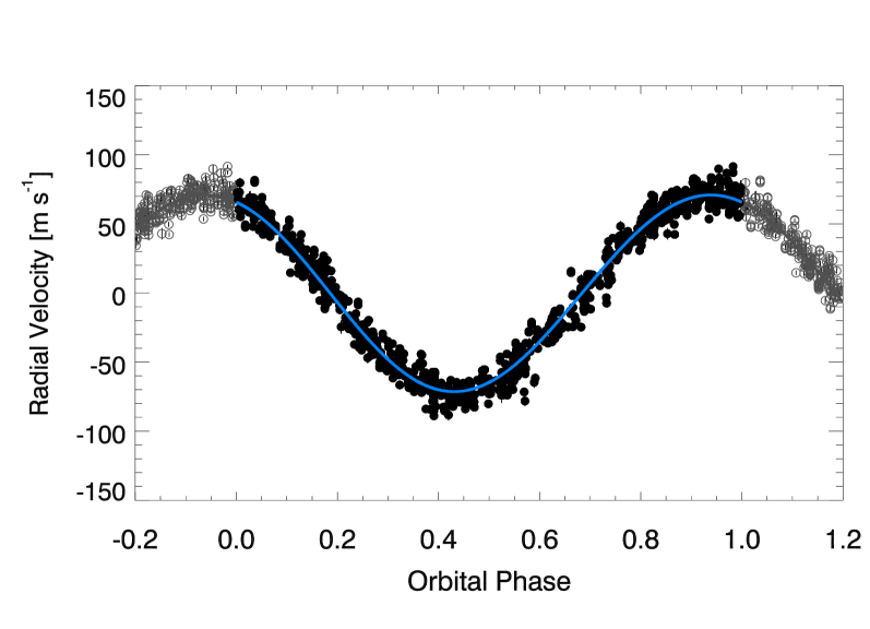
Figure 1: 55 Cnc b, phase-folded at 14.65194 days. The amplitude of 70.9 m s^-1 implies a planet with $M\sin i=0.81M_{Jup}$. Theoretical curve is overplotted as a blue line.

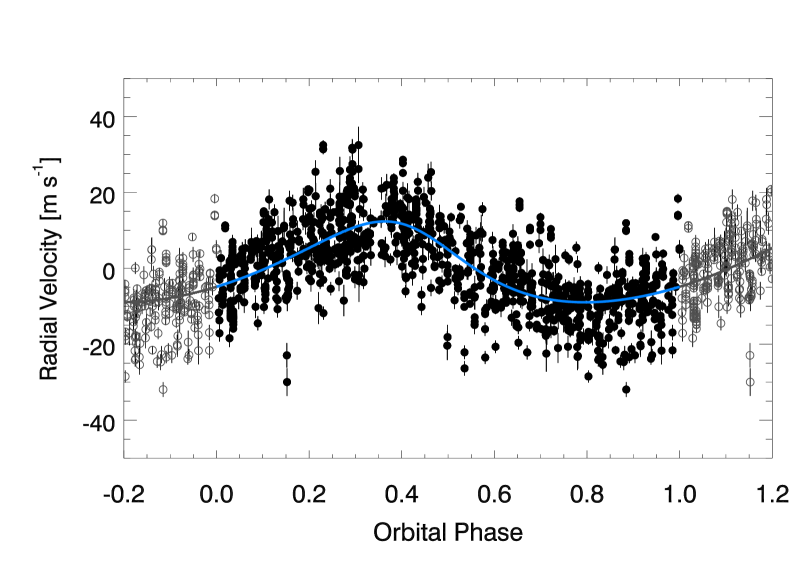
Figure 2: Radial velocities for 55 Cnc c, phase-folded at 44.392 days. The 10.6 m s^-1 amplitude corresponds to a $M\sin i=55.6M_{\oplus}$ planet. Model fit is overplotted as a blue line.

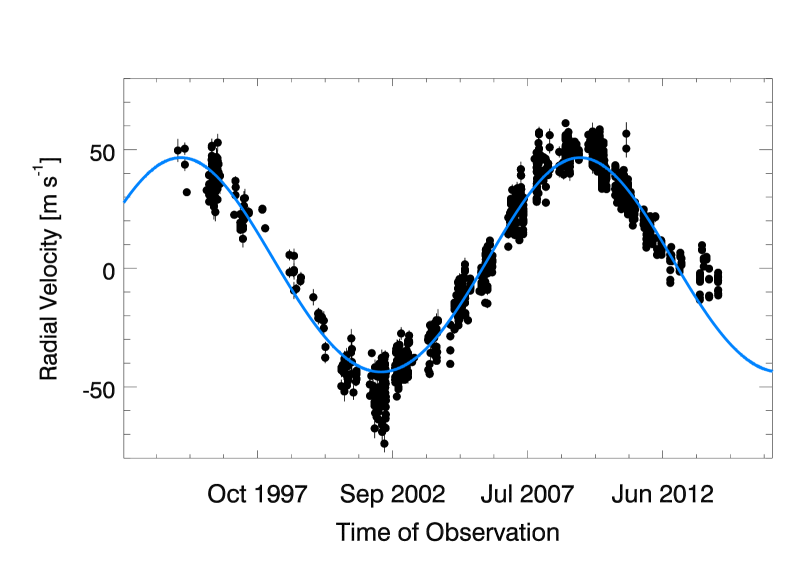
Figure 3: The time series data for 55 Cnc d with other planets removed, corresponds to a planet with an orbital period of 14.5 years and $M\sin i=3.7M_{Jup}$. Keplerian fit is overplotted as a blue line.

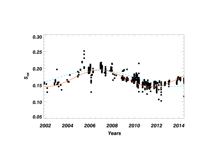
Figure 4: The magnetic activity cycle of 55 Cnc appears in the time series Ca II H&K emission from the Keck spectra. Consistent with the predicted correlation, the best fit period for $P_{cyc}$ is a 10 year period (red sinusoidal line). The 14.5 year period of the outer planet (rescaled and shown as a blue dashed line) is not in phase with the activity cycle.

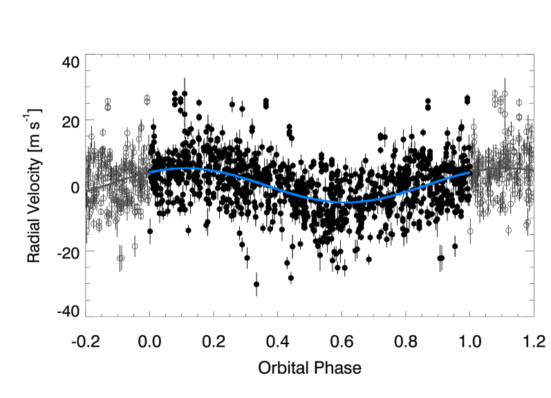
Figure 5: The 55 Cnc velocities are phase-folded at 0.73655 days revealing 5.7 m s^-1 signal that is modeled as 55 Cnc e, a $7.5M_{\oplus}$ planet. Model fit is overplotted as a blue line.

Figure 6: After fitting for planets b, c, d, e, a periodogram of the residual velocities shows a strong peak at 260 d.

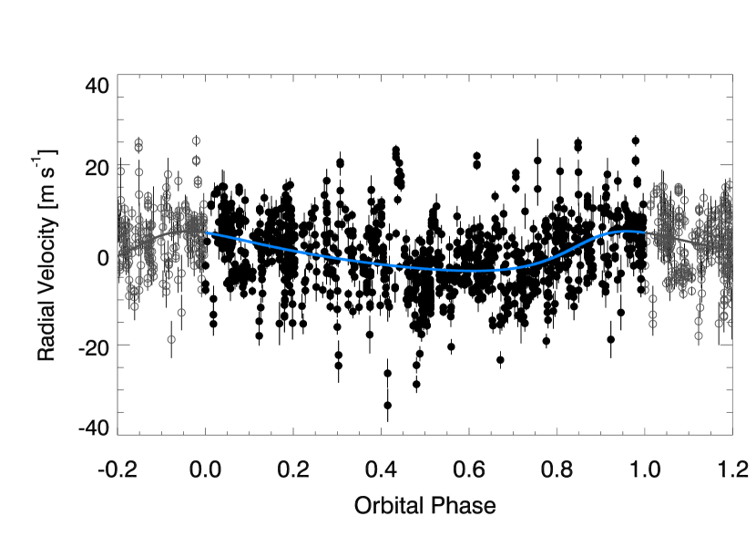
Figure 7: The radial velocity data are phase-folded at the best fit period of 259.4 days for 55 Cnc f. Theoretical fit is overplotted as a blue line.

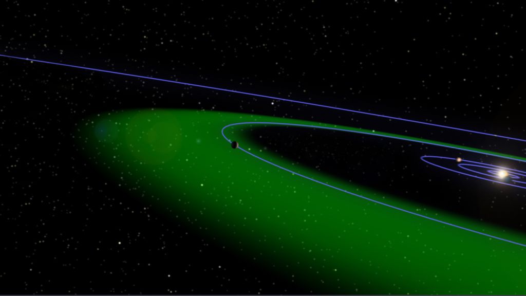
Figure 8: Artists rendition of the 55 Cnc exoplanet architecture, with 55 Cnc f in the habitable zone of the star.

4 A Transiting Planet

The change in orbital period from 2.8 days (McArthur et al. 2004) to 0.74 days (Dawson & Fabrycky 2010) doubled the probability of detecting a transit. Demory et al. (2011) estimated a transit probability of 29% for the revised orbital period and observed 55 Cnc at the predicted transit time on 6 January 2011 (Figure LABEL:fig:fig9) using the IRAC 4.5 micron channel on the warm Spitzer space telescope. A month later, Winn et al. (2011) carried out nearly continuous photometric monitoring of the system with the MOST (Microvariability and Oscillations of Stars) Canadian satellite from 2011 February 7 to 22. Both teams detected a transit at the time predicted with the shorter orbital period and adopted the careful interferometric measurement of the stellar angular diameter using the CHARA array (von Braun et al. 2011) to derive a radius for the planet.

Winn et al. 2011 modeled their phase-folded data (Figure LABEL:fig:fig10) and measured a transit depth of $380\pm 52$ ppm, implying a planet radius of $2.00\pm 14R_{\oplus}$. Adopting the stellar mass of $0.963^{+0.051}_{-0.029}$ from (Takeda et al. 2007) and stellar radius of $0.943\pm 0.01\,R_{\odot}$ they derived a planetary mass of $8.63M_{\oplus}$. Gillon et al. (2012) combined MOST observations with their new 4.5 $\mu$m Warm Spitzer IRAC data to derive a slightly larger radius of $2.17\pm 0.10R_{\oplus}$. This slightly larger radius leads them to conclude that 55 Cnc e has a gaseous envelope overlying a rocky nucleus. Given the proximity of the planet to the host star, the authors note that a plausible composition for the envelope is water in super-critical form. While the photometric errors from ground-based facilities are larger because of atmospheric scintillation, de Mooij et al. (2014) were able to detect the transit using ALFOSC with the 2.5-m Nordic Optical Telescope.

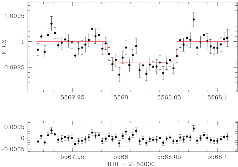
Figure 9: Demory et al. (2011) Spitzer transit of 55 Cnc e

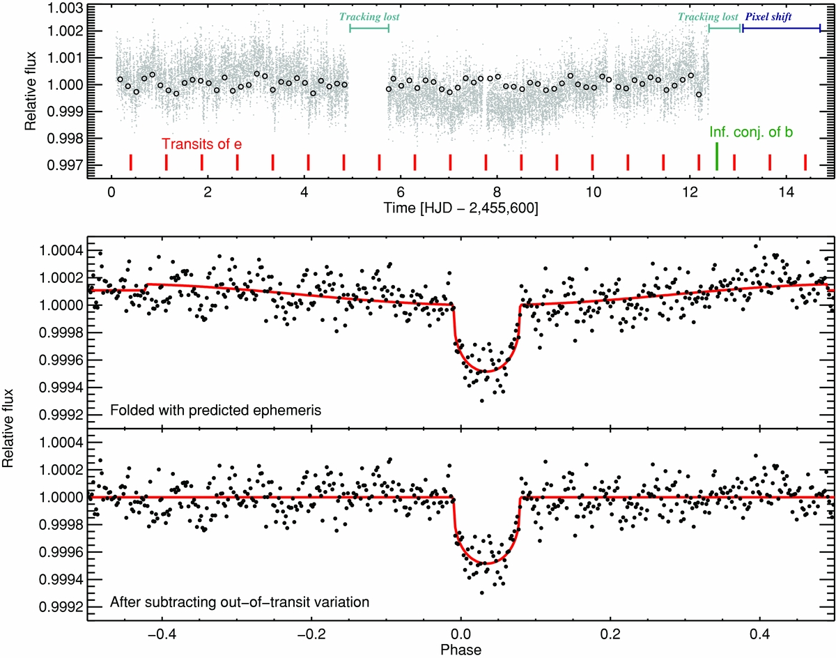
Figure 10: Winn et al. (2011) transit light curve from the MOST satellite, phase folded at P=0.74 d.

4.1 The Mistaken Identity of 55 Cnc e

With revised orbital parameters and a secure mass and radius for 55 Cnc e, the characterization of the planet has been the subject of lively debate. In particular, the ratio of carbon to oxygen in the protoplanetary disk influences the composition and structure of exoplanets. If ${\rm C/O}$ is above a threshold value, then carbonates will dominate (Brewer & Fischer 2016; Madhusudhan 2012). Conversely, the planet composition will be primarily magnesium silicates if ${\rm C/O}$ is below that threshold. The nominal threshold value is $\sim 1$ at the formation site of planetesimals, but with planetesimal migration, the threshold value could be as low as 0.6 (Moriarty et al. 2014). The stellar abundance ${\rm C/O}$ ratio is a reasonable estimate of the volatile gas ratio in the protoplanetary disk, and early estimates of ${\rm C/O}$ for 55 Cnc were as high as 1.12 (Delgado Mena et al. 2010) leading Madhusudhan et al. (2012) to consider the possibility of a carbon-rich interior structure for 55 Cnc e. The stellar ${\rm C/O}$ ratio has since been revised (Brewer et al. 2016) and Demory et al. (2016) provide a revised model for the interior structure of 55 Cnc e that is consistent with a iron core and silicate mantle, similar to Earth.

4.2 The Future

Our understanding of the planetary system orbiting 55 Cnc is likely to be revised again in the future. There is an enormous gap between 55 Cnc f orbiting at 0.78 AU and 55 Cnc d orbiting at 5.8 AU. If Nature abhors a vacuum, then there are sure to be additional planets awaiting discovery.