Fluctuation theorem for quantum-state statistics

Abstract

We derive the fluctuation theorem for quantum-state statistics that can be obtained when we initially measure the total energy of a quantum system at thermal equilibrium, let the system evolve unitarily, and record the quantum-state data reconstructed at the end of the process. The obtained theorem shows that the quantum-state statistics for the forward and backward processes is related to the equilibrium free-energy difference through an infinite series of independent relations, which gives the quantum work fluctuation theorem as a special case, and reproduces the out-of-time-order fluctuation-dissipation theorem near thermal equilibrium. The quantum-state statistics exhibits a system-size scaling behavior that differs between integrable and non-integrable (quantum chaotic) systems as demonstrated numerically for one-dimensional quantum lattice models.

Fluctuation theorems (FTs) have played a central role in our understanding of how macroscopic irreversibility arises from microscopically reversible equation of motion Boc ; Evans et al. (1993); Gallavotti and Cohen (1995); Jarzynski (1997); Crooks (1999); Esposito et al. (2009); Campisi et al. (2011). The FTs lead to many fundamental relations in thermodynamics and statistical mechanics, including the second law of thermodynamics, the fluctuation-dissipation theorem (FDT) Callen and Welton (1951); Kubo (1957); Marconi et al. (2008), and Onsager’s reciprocity relation Onsager (1931); Casimir (1945).

The conventional approach to FTs in isolated quantum systems is based on the two-point measurement for work Kur ; Tas ; Esposito et al. (2009): one initially measures the total energy, let the system evolve according to a time-dependent Hamiltonian, and again measures the total energy at the end of the process. From the difference between the initial and final total energies, one can extract the work done on the system by an external force. The obtained work probability distributions for the forward and time-reversed processes are related to the equilibrium free-energy difference between the initial and final configurations (the quantum work FT). In this approach, one makes a projective energy measurement (with the outcome $E_{l}^{f}$ being the $l$th eigenenergy of the final Hamiltonian) on the final state $\hat{\rho}$, so that one obtains limited information on the quantum state $\hat{\rho}$ itself, i.e., only the diagonal information $\langle E_{l}^{f}|\hat{\rho}|E_{l}^{f}\rangle$ is available, where $|E_{l}^{f}\rangle$ is the energy eigenstate.

How does the quantum state $\hat{\rho}$ realized after the time evolution (including information on the off-diagonal elements $\langle E_{l}^{f}|\hat{\rho}|E_{m}^{f}\rangle$, $l\neq m$) fluctuate? Here, by fluctuations of the quantum state we mean that the state fluctuates depending on the result of the initial energy measurement. If we repeat the procedure to (i) prepare the initial thermal equilibrium state, (ii) measure the total energy, (iii) perform a unitary time evolution, and (iv) reconstruct the quantum state $\hat{\rho}$, we can operationally determine the statistics of quantum states (Fig. 1). When the above procedure is repeated sufficiently many times, we obtain duplicated copies of quantum states, with which we can in principle reconstruct the quantum state using the technique of the quantum-state tomography Par ; Lvovsky and Raymer (2009).

The statistics of quantum states is closely related to quantum chaos, or non-integrability, of the system, the characterization of which has been a long-standing issue in statistical mechanics Berry (1987); Haake (2010). Suppose that after the first measurement the quantum state is projected to a certain eigenstate of the initial Hamiltonian. Then the state evolves within a subspace of the total Hilbert space due to the presence of conserved quantities. For integrable systems, the number of conserved quantities is extensive, so that the size of the subspace is highly constrained. Hence we expect that the resulting behavior of the quantum-state statistics is different between integrable and non-integrable systems.

Another motivation to study the quantum-state statistics is the recent finding of the out-of-time-order FDT Tsuji et al. (2018a), which relates chaotic properties of the system and a nonlinear response function involving a time-reversed process, and can be viewed as a higher-order extension of the conventional FDT. Provided that the conventional FDT can be derived from the quantum work FT near equilibrium, it is thus a natural question what is the underlying law that leads to the out-of-time-order FDT if applied near equilibrium.

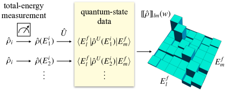
Figure 1: Schematic procedure for measuring quantum-state statistics. We initially prepare the thermal equilibrium state $\hat{\rho}_{i}$, and measure the total energy with the outcome $E_{k}^{i}$, where the state changes to $\hat{\rho}(E_{k}^{i})$. Then the system evolves according to a unitary operator $\hat{U}$, and the final state $\hat{\rho}^{U}(E_{k}^{i})$ is reconstructed in the energy eigenbasis. We repeat the procedure to accumulate the matrix data $[\![\hat{\rho}]\!]_{lm}(w)$ [Eq. (1)].

In this paper, we show that the quantum-state statistics accumulated under a certain condition for the forward and time-reversed processes satisfies an infinite series of exact relations that are expressed in terms of the equilibrium free-energy difference between the initial and final configurations. The relations include the quantum work (Crooks) FT as a special case, and allow further extensions. Near equilibrium, the out-of-time-order FDT Tsuji et al. (2018a) is reproduced. We argue that the fluctuation of the quantum-state statistics shows a different system-size scaling between integrable and non-integrable systems, which can be used as a diagnosis of quantum chaos. This is demonstrated numerically for one-dimensional quantum lattice models.

Let us suppose that an isolated quantum system evolves in time according to the time-dependent Hamiltonian $\hat{H}(s)$ ($t_{i}\leq s\leq t_{f}$) (forward process). The initial and final Hamiltonians are denoted by $\hat{H}_{i}=\hat{H}(t_{i})$ and $\hat{H}_{f}=\hat{H}(t_{f})$. The unitary evolution operator is given by $\hat{U}=\mathcal{T}\exp(-\frac{i}{\hbar}\int_{t_{i}}^{t_{f}}ds\,\hat{H}(s))$, where $\mathcal{T}$ represents the time-ordered product. We assume that the initial state is in thermal equilibrium with temperature $k_{B}T=\beta^{-1}$, and is described by the canonical ensemble with the density matrix $\hat{\rho}_{i}=e^{-\beta\hat{H}_{i}}/Z_{i}(\beta)$, where $Z_{i}(\beta)\equiv{\rm Tr}(e^{-\beta\hat{H}_{i}})$ is the partition function. We denote the eigenvalues and orthonormal eigenvectors of $\hat{H}_{i}$ ($\hat{H}_{f}$) by $E_{k}^{i}$ ($E_{k}^{f}$) and $|E_{k}^{i}\rangle$ ($|E_{k}^{f}\rangle$), respectively.

Suppose that we perform a projective energy measurement and obtain the measurement outcome $E_{k}^{i}$ with the probability $p_{k}^{i}=e^{-\beta E_{k}^{i}}/Z_{i}(\beta)$, where the quantum state $\hat{\rho}_{i}$ is projected from $\hat{\rho}_{i}$ to $\hat{\rho}(E_{k}^{i})=|E_{k}^{i}\rangle\langle E_{k}^{i}|$. After the unitary time evolution, the quantum state becomes $\hat{\rho}^{U}(E_{k}^{i})\equiv\hat{U}\hat{\rho}(E_{k}^{i})\hat{U}^{\dagger}$. At the end of the process, we record the quantum state reconstructed in the eigenbasis of the final Hamiltonian as $\langle E_{l}^{f}|\hat{\rho}^{U}(E_{k}^{i})|E_{m}^{f}\rangle$. We here address the question of whether there is any law that governs the statistics of these quantum-state data when we repeat the above procedure. We show that it emerges when we accumulate the quantum-state data under a certain energy constraint given by $w=\frac{1}{2}(E_{l}^{f}+E_{m}^{f})-E_{k}^{i}$. After taking the average, we obtain

$$[\![\hat{\rho}]\!]_{lm}(w)\equiv\overline{\delta(w-(\tfrac{1}{2}(E_{l}^{f}+E_{m}^{f})-E_{k}^{i}))\langle E_{l}^{f}|\hat{\rho}^{U}(E_{k}^{i})|E_{m}^{f}\rangle}$$

$$=\sum_{k}p_{k}^{i}\delta(w-(\tfrac{1}{2}(E_{l}^{f}+E_{m}^{f})-E_{k}^{i}))\langle E_{l}^{f}|\hat{\rho}^{U}(E_{k}^{i})|E_{m}^{f}\rangle,$$ (1)

where the overline represents the average over the repeated processes, and $\delta(x)$ is the Dirac delta function. For $l=m$, $w$ corresponds precisely to the difference between the initial and final energies, which is equivalent to the work performed on the system. However, for off-diagonal elements, $w$ does not, in general, correspond to the work, but only has a formal meaning of the difference between the initial energy $E_{k}^{i}$ and the averaged final energy $\frac{1}{2}(E_{l}^{f}+E_{m}^{f})$.

We also consider the time-reversed process with the Hamiltonian $\hat{\bar{H}}(s)=\Theta\hat{H}(t_{i}+t_{f}-s)\Theta^{-1}$ ($t_{i}\leq s\leq t_{f}$), where $\Theta$ represents the antiunitary time-reversal operator. The corresponding initial and final Hamiltonians are $\hat{\bar{H}}_{i}=\hat{\bar{H}}(t_{i})$ and $\hat{\bar{H}}_{f}=\hat{\bar{H}}(t_{f})$, and the unitary evolution is given by $\hat{\bar{U}}=\Theta\hat{U}^{\dagger}\Theta^{-1}$. The initial state for the time-reversed process is assumed to be $\hat{\bar{\rho}}_{i}=e^{-\beta\hat{\bar{H}}_{i}}/\bar{Z}_{i}(\beta)$, where $\bar{Z}_{i}(\beta)={\rm Tr}(e^{-\beta\hat{\bar{H}}_{i}})$. In the same way as the forward process, we define

$$[\![\hat{\bar{\rho}}]\!]_{lm}(w)\equiv\overline{\delta(w-(\tfrac{1}{2}(\bar{E}_{l}^{f}+\bar{E}_{m}^{f})-\bar{E}_{k}^{i}))\langle\bar{E}_{l}^{f}|\hat{\bar{\rho}}^{\bar{U}}(\bar{E}_{k}^{i})|\bar{E}_{m}^{f}\rangle}$$

$$=\sum_{k}\bar{p}_{k}^{i}\delta(w-(\tfrac{1}{2}(\bar{E}_{l}^{f}+\bar{E}_{m}^{f})-\bar{E}_{k}^{i}))\langle\bar{E}_{l}^{f}|\hat{\bar{\rho}}^{\bar{U}}(\bar{E}_{k}^{i})|\bar{E}_{m}^{f}\rangle,$$ (2)

where $\bar{E}_{k}^{i}$ ($\bar{E}_{k}^{f}$) and $|\bar{E}_{k}^{i}\rangle$ ($|\bar{E}_{k}^{f}\rangle$) are the eigenvalues and orthonormal eigenvectors of $\hat{\bar{H}}_{i}$ ($\hat{\bar{H}}_{f}$), respectively, $\bar{p}_{k}^{i}=e^{-\beta\bar{E}_{k}^{i}}/\bar{Z}_{i}(\beta)$, $\hat{\bar{\rho}}^{\bar{U}}(\bar{E}_{k}^{i})=\hat{\bar{U}}\hat{\bar{\rho}}(\bar{E}_{k}^{i})\hat{\bar{U}}^{\dagger}$, and $\hat{\bar{\rho}}(\bar{E}_{k}^{i})=|\bar{E}_{k}^{i}\rangle\langle\bar{E}_{k}^{i}|$.

Since $[\![\hat{\rho}]\!](w)$ is an operator acting on the Hilbert space, there are various ways to retrieve information from this object. Let us define distribution functions for the quantum-state statistics by taking the trace of the $n$th moment of $[\![\hat{\rho}]\!](w)$ ($n=1,2,\dots$),

$$p_{n}(w) \equiv\frac{1}{\mathcal{N}_{n}}{\rm Tr}([\![\hat{\rho}]\!]^{\circledast n}(w)).$$ (3)

Here $\mathcal{N}_{n}$ is a normalization constant determined by

$$\int_{-\infty}^{\infty}dw\,p_{n}(w) =1,$$ (4)

and $[\![\hat{\rho}]\!]^{\circledast n}(w)=([\![\hat{\rho}]\!]\circledast\cdots\circledast[\![\hat{\rho}]\!])(w)$ is defined by the $n$th power of $[\![\hat{\rho}]\!](w)$ with the symbol $\circledast$ denoting the matrix multiplication and energy convolution simultaneously, i.e.,

$$([\![\hat{\rho}]\!]\circledast[\![\hat{\rho}]\!])_{lm}(w) \equiv\int_{-\infty}^{\infty}dw^{\prime}\sum_{n}[\![\hat{\rho}]\!]_{ln}(w-w^{\prime})[\![\hat{\rho}]\!]_{nm}(w^{\prime}).$$ (5)

For the time-reversed process, the corresponding distribution function is defined by $\bar{p}_{n}(w)\equiv\frac{1}{\bar{\mathcal{N}}_{n}}{\rm Tr}([\![\hat{\bar{\rho}}]\!]^{\circledast n}(w))$ with the normalization condition $\int_{-\infty}^{\infty}dw\,\bar{p}_{n}(w)=1$ and $\bar{\mathcal{N}}_{n}$ being the normalization constant for $\bar{p}_{n}(w)$.

At $n=1$, $p_{n}(w)$ is identical to the work probability distribution: $p_{1}(w)=\sum_{kl}p_{k}^{i}\delta(w-E_{l}^{f}+E_{k}^{i})|\langle E_{l}^{f}|\hat{U}|E_{k}^{i}\rangle|^{2}$. For arbitrary $n$, $p_{n}(w)$ can be proven to take a real value (Appendix A). However, for $n\geq 2$, $p_{n}(w)$ is not necessarily positive semidefinite. This prevents us from interpreting $p_{n}(w)$ ($n\geq 2$) as a probability distribution, though $p_{n}(w)$ satisfies the normalization condition (4). Hence $p_{n}(w)$ ($n\geq 2$) should be regarded as a quasiprobability.

The main result of this paper is that the following relation holds between $p_{n}(w)$ and its time-reversed partner $\bar{p}_{n}(w)$:

$$\frac{p_{n}(w)}{\bar{p}_{n}(-w)} =e^{\beta(w-n\Delta F(n\beta))}\quad(n=1,2,\dots).$$ (6)

Here $\Delta F(\beta)=F_{f}(\beta)-F_{i}(\beta)$ [$F_{i,f}(\beta)=-\beta^{-1}\ln Z_{i,f}(\beta)$] is the difference of the equilibrium free energies for the initial and final Hamiltonians at temperature $\beta^{-1}$. Note that the inverse temperature appearing in the free-energy argument is multiplied by $n$ in Eq. (6). For $n=1$, the relation (6) reduces to the quantum work FT, $p_{1}(w)/\bar{p}_{1}(-w)=e^{\beta(w-\Delta F(\beta))}$. For $n\geq 2$, the relation (6) gives an extension of the FT to the quantum-state statistics. A remarkable feature of Eq. (6) is that it is valid for arbitrary unitary evolution $\hat{U}$, no matter how the system is driven away from equilibrium. Note that on the left-hand side of Eq. (6) each $p_{n}(w)$ and $\bar{p}_{n}(-w)$ strongly depends on $\hat{U}$, while the right-hand side is written in terms of the equilibrium quantities.

The relation (6) can be derived using the method of characteristic functions Talkner et al. (2007). Here we define a characteristic function for $p_{n}(w)$ as the Fourier transform of $p_{n}(w)$,

$$G_{n}(u) \equiv\int_{-\infty}^{\infty}dw\,e^{iuw}p_{n}(w),$$ (7)

which can be written as $G_{n}(u)=\mathcal{N}_{n}^{-1}{\rm Tr}[(\hat{\rho}_{i}\hat{W}_{i,u}^{\dagger}(t_{i})\hat{W}_{f,u}(t_{f})^{n})]$, where $\hat{W}_{i,u}(t_{i})$ and $\hat{W}_{f,u}(t_{f})$ are the Heisenberg representation of operators $\hat{W}_{i,u}\equiv e^{iu\hat{H}_{i}}$ and $\hat{W}_{f,u}\equiv e^{iu\hat{H}_{f}}$, respectively (Appendix A). Hence $G_{n}(u)$ ($n\geq 2$) is classified into an out-of-time-ordered correlation function Lar . By using the time-reversal property of $G_{n}(u)$, we find a symmetry relation $G_{n}(u)=(Z_{f}(n\beta)/Z_{i}(n\beta))\bar{G}_{n}(-u+i\beta)$, where $\bar{G}_{n}(u)$ is the characteristic function for $\bar{p}_{n}(w)$. After Fourier transformation, we arrive at Eq. (6). The details of the proof is described in Appendix A.

By multiplying $e^{-\beta w}\bar{p}_{n}(-w)$ on both sides of Eq. (6) and using the normalization condition (4), we obtain the integral FT for the quantum-state statistics,

$$\langle e^{-\beta w}\rangle_{p_{n}} =e^{-n\beta\Delta F(n\beta)},$$ (8)

where $\langle\cdots\rangle_{p_{n}}\equiv\int_{-\infty}^{\infty}dw\,p_{n}(w)\cdots$. For $n=1$, the relation (8) is nothing but the Jarzynski equality, $\langle e^{-\beta w}\rangle_{p_{1}}=e^{-\beta\Delta F(\beta)}$, while for $n\geq 2$ it provides an extension of the Jarzynski equality. If one knows the distribution function $p_{n}(w)$, one can extract the equilibrium free-energy difference at temperature $k_{B}T/n=(n\beta)^{-1}$. Since $p_{n}(w)$ is generated by the characteristic function $G_{n}(u)$, one can measure $p_{n}(w)$ through the measurement of the out-of-time-ordered correlation function, for which various protocols have been proposed Swingle et al. (2016); Campisi and Goold (2017); Yao ; Zhu et al. (2016); Tsuji et al. (2017, 2018a); Yunger Halpern (2017); Yunger Halpern et al. (2018).

Applying Jensen’s inequality to the Jarzynski equality, one arrives at the second law of thermodynamics,

$$\langle w\rangle_{p_{1}} \geq\Delta F(\beta).$$ (9)

One may wonder if one could derive a similar inequality

$$\langle w\rangle_{p_{n}}\geq n\Delta F(n\beta)\quad(!)$$ (10)

from Eq. (8). This is, however, possible only if $p_{n}(w)$ is positive semidefinite, since one cannot use Jensen’s inequality for non-positive-semidefinite distributions. We note that $p_{n}(w)$ becomes positive semidefinite in the zero-temperature limit ($\beta\to\infty$). Let us assume that the ground state of the initial system (denoted by $|E_{g}^{i}\rangle$ with the eigenenergy $E_{g}^{i}$) is unique. Then, in the zero-temperature limit,

$$p_{n}(w) \to\frac{1}{\mathcal{N}_{n}}\sum_{l_{1},\dots,l_{n}}\delta(w-(E_{l_{1}}^{f}+\cdots+E_{l_{n}}^{f})+nE_{g}^{i})(p_{g}^{i})^{n}$$

$$\quad\times|\langle E_{l_{1}}^{f}|\hat{U}|E_{g}^{i}\rangle|^{2}\cdots|\langle E_{l_{n}}^{f}|\hat{U}|E_{g}^{i}\rangle|^{2}\geq 0$$ (11)

with $p_{g}^{i}=e^{-\beta E_{g}^{i}}/Z_{i}(\beta)$. Thus, at zero temperature the inequality (10) holds. Of course, this does not mean that we have a new second law in addition to the existing one (9). At zero temperature $p_{n}(w)$ is related to $p_{1}(w)$ through $p_{n}(w)=\int_{-\infty}^{\infty}dw_{1}\cdots dw_{n-1}\,p_{1}(w-w_{1})p_{1}(w_{1}-w_{2})\cdots p_{1}(w_{n-2}-w_{n-1})p_{1}(w_{n-1})$, from which one obtains $\langle w\rangle_{p_{n}}=n\langle w\rangle_{p_{1}}$. Therefore, the inequality (10) reduces to the second law (9) at zero temperature [where $\Delta F(n\beta)\sim\Delta F(\beta)$], and (10) does not provide new information in this case. In fact, the relation (6) reduces to the quantum work FT [Eq. (6) with $n=1$] in the zero-temperature limit. To obtain new information beyond the quantum work FT, one has to consider finite-temperature states.

If the relation (6) is applied near equilibrium, one can reproduce the out-of-time-order FDT Tsuji et al. (2018a) around zero frequency. This can be seen from the expansion of the integral FT (8) for $n=1$ and $n=2$ up to the third cumulants with respect to $w$. If the Hamiltonian is split into the time-independent part and the rest as $\hat{H}(s)=\hat{H}_{0}+\xi(s)\hat{X}(s)$, where $\xi(s)$ is an external field and $\hat{X}(s)$ is the coupled operator, then the second-order functional derivative $\frac{\delta^{2}}{\delta\xi(s)\xi(s^{\prime})}$ on both sides of the cumulant expansions around $\xi(s)=0$ (near equilibrium) leads to the near-zero-frequency part of the out-of-time-order FDT. Details of the derivation are given in Appendix B.

We have examined two aspects of $p_{n}(w)$: the distribution function for the quantum-state statistics and out-of-time-ordered correlation functions. For the latter, there have been various discussions in relation to chaotic properties of quantum systems Kit ; Mal ; Swingle et al. (2016); Rozenbaum et al. (2017); Aleiner et al. (2016); Fan et al. (2017); Tsuji et al. (2018b). Here we argue that there is a strong connection between the fluctuation in $p_{n}(w)$ ($n\geq 2$) and quantum chaotic nature (non-integrability) of the system. The crucial difference of $p_{n}(w)$ ($n\geq 2$) from the work probability distribution $p_{1}(w)$ is that the former can take a negative value. In the following, we focus on the case of $n=2$. We quantify the fluctuation in $p_{2}(w)$ by the $L^{1}$ norm ($\|\cdot\|_{1}$),

$$\Delta p_{2} \equiv\frac{1}{Z_{i}(\beta)}\|p_{2}(w)\|_{1}=\frac{1}{Z_{i}(\beta)}\int_{-\infty}^{\infty}dw\,|p_{2}(w)|.$$ (12)

$\Delta p_{2}$ counts the negative portion of $p_{2}(w)$ since $\Delta p_{2}=Z_{i}(\beta)^{-1}[1-2\int_{p_{2}(w)<0}dw\,p_{2}(w)]$ (note that $p_{2}(w)$ satisfies the normalization condition (4)).

As an illustration, let us consider the case that the Hamiltonian is suddenly quenched (i.e., $\hat{H}(s)=\hat{H}_{i}\to\hat{H}_{f}$) and the initial temperature is $\beta=0$. If we assume a non-degeneracy condition (Appendix C), $\Delta p_{2}$ is written for real Hamiltonians as $\Delta p_{2}=Z_{i}(0)^{-2}\sum_{klmn}|\langle E_{k}^{i}|E_{n}^{f}\rangle|\cdot|\langle E_{n}^{f}|E_{m}^{i}\rangle|\cdot|\langle E_{m}^{i}|E_{l}^{f}\rangle|\cdot|\langle E_{l}^{f}|E_{k}^{i}\rangle|$. Using conserved quantities inherent in the system, the unitary transition matrix $\hat{U}_{lk}\equiv\langle E_{l}^{f}|E_{k}^{i}\rangle$ can be block-diagonalized as $\hat{U}=\oplus_{\alpha}\hat{U}^{(\alpha)}$. If we define an entrywise-absolute-value matrix, $(\hat{U}_{\rm abs}^{(\alpha)})_{lk}\equiv|\hat{U}_{lk}^{(\alpha)}|$, then $\Delta p_{2}=Z_{i}(0)^{-2}\sum_{\alpha}{\rm Tr}(\hat{U}_{\rm abs}^{(\alpha)\dagger}\hat{U}_{\rm abs}^{(\alpha)}\hat{U}_{\rm abs}^{(\alpha)\dagger}\hat{U}_{\rm abs}^{(\alpha)})=Z_{i}(0)^{-2}\sum_{\alpha}\|\hat{U}_{\rm abs}^{(\alpha)\dagger}\hat{U}_{\rm abs}^{(\alpha)}\|_{F}^{2}$, where $\|\cdot\|_{F}$ denotes the Frobenius norm. Since the Frobenius norm is submultiplicative, $\Delta p_{2}$ satisfies an inequality, $\Delta p_{2}\leq Z_{i}(0)^{-2}\sum_{\alpha}\|\hat{U}_{\rm abs}^{(\alpha)\dagger}\|_{F}^{2}\|\hat{U}_{\rm abs}^{(\alpha)}\|_{F}^{2}$. By using the relation $\|\hat{U}_{\rm abs}^{(\alpha)}\|_{F}^{2}=\|\hat{U}_{\rm abs}^{(\alpha)\dagger}\|_{F}^{2}=\|\hat{U}^{(\alpha)}\|_{F}^{2}={\rm Tr}(\hat{U}^{(\alpha)}\hat{U}^{(\alpha)\dagger})=D_{\alpha}$ ($D_{\alpha}$ is the dimension of the $\alpha$th block Hilbert space) and $Z_{i}(0)=\sum_{\alpha}D_{\alpha}=D$ ($D$ is the dimension of the total Hilbert space), we obtain

$$\Delta p_{2} \leq\frac{\sum_{\alpha}D_{\alpha}^{2}}{(\sum_{\alpha}D_{\alpha})^{2}}.$$ (13)

The right-hand side of this inequality strongly depends on the number of conserved quantities. As an estimate, let’s suppose that each block Hilbert space has approximately the same dimension (i.e., $D_{\alpha}$ is independent of $\alpha$). Then $\Delta p_{2}\lesssim D_{\alpha}/D$, i.e., the fluctuation in $p_{2}(w)$ is constrained by the dimension of the block Hilbert space as compared to the dimension of the total Hilbert space. In integrable systems, the number of conserved quantities typically grows in proportion to the system size, so that $D_{\alpha}/D$ is expected to decay exponentially in the large system-size limit. On the other hand, in non-integrable systems there is a finite number of conserved quantities, so that $D_{\alpha}/D$ remains constant (or decays at most algebraically) as the system size increases. One can thus distinguish integrable and non-integrable systems by examining the system-size scaling behavior of $\Delta p_{2}$.

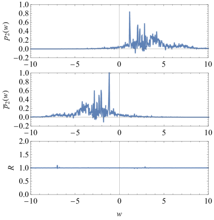
Figure 2: Plot of $p_{2}(w)$ for the forward process (3) (top panel) and that of $\bar{p}_{2}(w)$ for the time-reversed process (middle) in the one-dimensional hard-core boson model (14) driven by the interaction quench $V=2\to 4$ with $t^{\prime}=V^{\prime}=1$, $\beta=0.1$, $L=12$, and $N=4$. The bottom panel plots $R=p_{2}(w)/\bar{p}_{2}(-w)/e^{\beta(w-2\Delta F(2\beta))}$ as a function of $w$. The finite-size grid ($\Delta w=0.04$) is used.

We numerically demonstrate the relation (6) for the quantum-state statistics and the behavior of $\Delta p_{2}$ (12) for the one-dimensional model of hard-core bosons with the Hamiltonian,

$$\hat{H}(s) =-t\sum_{i}(b_{i}^{\dagger}b_{i+1}+\mbox{h.c.})+V(s)\sum_{i}n_{i}^{b}n_{i+1}^{b}$$

$$\quad-t^{\prime}\sum_{i}(b_{i}^{\dagger}b_{i+2}+\mbox{h.c.})+V^{\prime}\sum_{i}n_{i}^{b}n_{i+2}^{b},$$ (14)

where $t$ ($t^{\prime}$) and $V(s)$ ($V^{\prime}$) are the (next-)nearest-neighbor hopping and the strength of the interaction, respectively, and $b_{i}^{\dagger}$ is the creation operator for hard-core bosons at site $i$. We use $t$ as the unit of energy, and assumes the periodic boundary condition. The results are shown for the filling $N/L=1/3$, where $N$ and $L$ are the number of particles and lattice sites, respectively. For other fillings, we obtain qualitatively similar results (Appendix C). To drive the system out of equilibrium, we perform an interaction quench $V(s)=V_{i}\to V_{f}$ at time $s=0$. In this setup, $p_{n}(w)$ (3) does not depend on $t_{i}(<0)$ and $t_{f}(>0)$. We numerically solve the model by exact diagonalization (for details, see Appendix C).

The model (14) has been well studied in the context of quantum chaos Rigol (2009a); Santos and Rigol (2010). At $t^{\prime}=V^{\prime}=0$, the model is known to be integrable. In the non-integrable case ($t^{\prime}\neq 0$ or $V^{\prime}\neq 0$), the level-spacing statistics shows the Wigner-Dyson distribution, which is the universal property of quantum chaotic systems as expected from random matrix theory. The non-integrable model satisfies the eigenstate thermalization hypothesis Deutsch (1991); Srednicki (1994); Rigol et al. (2008), which is a sufficient condition for an isolated quantum system to be thermalized.

In the top and middle panels in Fig. 2, we plot the distribution functions $p_{2}(w)$ for the forward process and $\bar{p}_{2}(w)$ for the time-reversed processes with $\beta=0.1$, where we take a finite grid size $\Delta w=0.04$ to broaden the delta function (Appendix C). We clearly see that both $p_{2}(w)$ and $\bar{p}_{2}(w)$ have negative parts. In the bottom panel of Fig. 2, we plot $R\equiv p_{2}(w)/\bar{p}_{2}(-w)/e^{\beta(w-2\Delta F(2\beta))}$. The value of $R$ stays close to $1$ over the whole region of $w$, which confirms the validity of the FT (6) for the quantum-state statistics. Small derivations are due to the finite grid $\Delta w$ used to plot $p_{2}(w)$ and $\bar{p}_{2}(w)$.

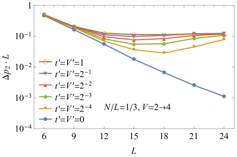
Figure 3: Log plot of $\Delta p_{2}\cdot L$ against the system size $L$ for the one-dimensional hard-core boson model (14) with $\beta=0$ driven by the interaction quench $V=2\to 4$. The system is integrable if $t^{\prime}=V^{\prime}=0$ and non-integrable otherwise.

We numerically evaluate $\Delta p_{2}$ (12), which quantifies the negative portion of the distribution $p_{2}(w)$, for the one-dimensional hardcore boson model (14) in the limit of $\Delta w\to 0$ while keeping $L$ fixed (Appendix C). At zero temperature, $p_{2}(w)$ is positive semidefinite (i.e., $\Delta p_{2}=Z_{i}(\beta)^{-1}$) as explained earlier, and $\Delta p_{2}$ grows monotonically as temperature increases. In Fig. 3, we plot $\Delta p_{2}$ multiplied by the system size $L$ as a function of $L$ at $\beta=0$ for the quench $V=2\to 4$. Clearly, $\Delta p_{2}$ shows a different scaling behavior between the integrable ($t^{\prime}=V^{\prime}=0$) and non-integrable ($t^{\prime}=V^{\prime}\neq 0$) cases. For the integrable case, $\Delta p_{2}$ tends to decay exponentially (within $L\leq 24$ one can still see slight bending of the curve in the log plot in Fig. 3), while for the non-integrable cases $\Delta p_{2}$ decays algebraically ($\Delta p_{2}\propto L^{-1}$) and converges to the single universal curve. Even a tiny violation of integrability ($t^{\prime}=V^{\prime}=2^{-4}$) causes a big difference in the behavior of $\Delta p_{2}$. These results are consistent with the inequality (13). For the one-dimensional hardcore boson model (14), in the non-integrable case $D=\binom{L}{N}$ and $D_{\alpha}\approx\frac{1}{L}\binom{L}{N}$ due to the parity and translational symmetries. From (13), $\Delta p_{2}$ is roughly bounded by $\Delta p_{2}\lesssim L^{-1}$. If $\Delta p_{2}$ decays as a power law, $\Delta p_{2}\propto L^{-\gamma}$, then the exponent $\gamma$ must satisfy $\gamma\geq 1$. The results shown in Fig. 3 indicate that the inequality for the exponent $\gamma$ is saturated (i.e., $\gamma=1$). In the integrable case shown in Fig. 3, the numerical estimate within $L\leq 24$ suggests that $\Delta p_{2}\propto e^{-cL}$ with $c=0.30$, the value of which is, however, non-universal and depends on the model parameters. We also simulate the same quantity for the one-dimensional spinless fermion model with nearest and next nearest neighbor hopping and interaction Rigol (2009b); Santos and Rigol (2010), and obtain similar results (Appendix C).

To summarize, we have studied the statistics of quantum states that can be obtained by the projective energy measurement followed by unitary evolution and quantum-state reconstruction in the energy basis. By accumulating the data of quantum states under a certain energy condition [Eq. (1)], we obtain the distribution function [Eq. (3)] which satisfies an infinite series of exact relations [Eq. (6)] (fluctuation theorem for the quantum-state statistics). It contains the quantum work fluctuation theorem as a special case, and if applied near equilibrium it reproduces the out-of-time-order fluctuation-dissipation theorem Tsuji et al. (2018a), which connects chaotic properties of the system and a nonlinear response function. We have discussed various aspects of the distribution function for the quantum-state statistics. In particular, the negativity of the distribution is closely related to the quantum chaotic nature (non-integrability) of the underlying model Hamiltonian. We have numerically demonstrated this for one-dimensional integrable and non-integrable quantum lattice models. The implications of the obtained relations to thermodynamics and thermalization in isolated quantum systems merit further study.

Appendix A Proof of the fluctuation theorem for the quantum-state statistics

In this section, we prove the fluctuation theorem for the quantum-state statistics [Eq. (6)],

$$\frac{p_{n}(w)}{\bar{p}_{n}(-w)} =e^{\beta(w-n\Delta F(n\beta))}\quad(n=1,2,\dots).$$ (15)

The proof is actually similar to that for the ordinary quantum work fluctuation theorem using the method of characteristic functions Talkner et al. (2007).

Let us first recursively evaluate the product $\circledast$ in the definition of $p_{n}(w)$ in the energy eigenbasis,

$$p_{n}(w) =\frac{1}{\mathcal{N}_{n}}{\rm Tr}([\![\hat{\rho}]\!]^{\circledast n}(w))$$

$$=\frac{1}{\mathcal{N}_{n}}\sum_{k_{1},\cdots,k_{n}}\sum_{l_{1},\cdots,l_{n}}p_{k_{1}}^{i}p_{k_{2}}^{i}\cdots p_{k_{n}}^{i}\delta(w-(E_{l_{1}}^{f}+E_{l_{2}}^{f}+\cdots+E_{l_{n}}^{f})+(E_{k_{1}}^{i}+E_{k_{2}}^{i}+\cdots+E_{k_{n}}^{i}))$$

$$\quad\times\langle E_{l_{1}}^{f}|\hat{U}|E_{k_{1}}^{i}\rangle\langle E_{k_{1}}^{i}|\hat{U}^{\dagger}|E_{l_{2}}^{f}\rangle\langle E_{l_{2}}^{f}|\hat{U}|E_{k_{2}}^{i}\rangle\langle E_{k_{2}}^{i}|\hat{U}^{\dagger}|E_{l_{3}}^{f}\rangle\cdots\langle E_{l_{n}}^{f}|\hat{U}|E_{k_{n}}^{i}\rangle\langle E_{k_{n}}^{i}|\hat{U}^{\dagger}|E_{l_{1}}^{f}\rangle.$$ (16)

The normalization constant $\mathcal{N}_{n}$ is determined by the direct calculation of the integral of $p_{n}(w)$,

$$1 =\int_{-\infty}^{\infty}dw\,p_{n}(w)$$

$$=\frac{1}{\mathcal{N}_{n}}\sum_{k_{1},\cdots,k_{n}}\sum_{l_{1},\cdots,l_{n}}p_{k_{1}}^{i}p_{k_{2}}^{i}\cdots p_{k_{n}}^{i}\langle E_{l_{1}}^{f}|\hat{U}|E_{k_{1}}^{i}\rangle\langle E_{k_{1}}^{i}|\hat{U}^{\dagger}|E_{l_{2}}^{f}\rangle\langle E_{l_{2}}^{f}|\hat{U}|E_{k_{2}}^{i}\rangle\langle E_{k_{2}}^{i}|\hat{U}^{\dagger}|E_{l_{3}}^{f}\rangle\cdots\langle E_{l_{n}}^{f}|\hat{U}|E_{k_{n}}^{i}\rangle\langle E_{k_{n}}^{i}|\hat{U}^{\dagger}|E_{l_{1}}^{f}\rangle.$$

$$=\frac{1}{\mathcal{N}_{n}}\sum_{l_{1},\cdots,l_{n}}\langle E_{l_{1}}^{f}|\hat{U}\hat{\rho}_{i}\hat{U}^{\dagger}|E_{l_{2}}^{f}\rangle\langle E_{l_{2}}^{f}|\hat{U}\hat{\rho}_{i}\hat{U}^{\dagger}|E_{l_{3}}^{f}\rangle\cdots\langle E_{l_{n}}^{f}|\hat{U}\hat{\rho}_{i}\hat{U}^{\dagger}|E_{l_{1}}^{f}\rangle.$$

$$=\frac{1}{\mathcal{N}_{n}}{\rm Tr}[(\hat{U}\hat{\rho}_{i}\hat{U}^{\dagger})(\hat{U}\hat{\rho}_{i}\hat{U}^{\dagger})\cdots(\hat{U}\hat{\rho}_{i}\hat{U}^{\dagger})]=\frac{1}{\mathcal{N}_{n}}{\rm Tr}(\hat{\rho}_{i}^{n})=\frac{1}{\mathcal{N}_{n}}\frac{Z_{i}(n\beta)}{Z_{i}(\beta)^{n}}.$$ (17)

Hence $\mathcal{N}_{n}$ is given by the equilibrium partition function as

$$\mathcal{N}_{n} =\frac{Z_{i}(n\beta)}{Z_{i}(\beta)^{n}}.$$ (18)

In particular, $\mathcal{N}_{n}$ is real ($\mathcal{N}_{n}\in\mathbb{R}$). $p_{n}(w)$ is also real ($p_{n}(w)\in\mathbb{R}$) as confirmed by taking the complex conjugate of $p_{n}(w)$,

$$p_{n}(w)^{\ast} =\frac{1}{\mathcal{N}_{n}}\sum_{k_{1},\cdots,k_{n}}\sum_{l_{1},\cdots,l_{n}}p_{k_{1}}^{i}p_{k_{2}}^{i}\cdots p_{k_{n}}^{i}\delta(w-(E_{l_{1}}^{f}+E_{l_{2}}^{f}+\cdots+E_{l_{n}}^{f})+(E_{k_{1}}^{i}+E_{k_{2}}^{i}+\cdots+E_{k_{n}}^{i}))$$

$$\quad\times\langle E_{k_{1}}^{i}|\hat{U}^{\dagger}|E_{l_{1}}^{f}\rangle\langle E_{l_{2}}^{f}|\hat{U}|E_{k_{1}}^{i}\rangle\langle E_{k_{2}}^{i}|\hat{U}^{\dagger}|E_{l_{2}}^{f}\rangle\langle E_{l_{3}}^{f}|\hat{U}|E_{k_{2}}^{i}\rangle\cdots\langle E_{k_{n}}^{i}|\hat{U}^{\dagger}|E_{l_{n}}^{f}\rangle\langle E_{l_{1}}^{f}|\hat{U}|E_{k_{n}}^{i}\rangle$$

$$=\frac{1}{\mathcal{N}_{n}}\sum_{k_{1},\cdots,k_{n}}\sum_{l_{1},\cdots,l_{n}}p_{k_{1}}^{i}p_{k_{2}}^{i}\cdots p_{k_{n}}^{i}\delta(w-(E_{l_{1}}^{f}+E_{l_{2}}^{f}+\cdots+E_{l_{n}}^{f})+(E_{k_{1}}^{i}+E_{k_{2}}^{i}+\cdots+E_{k_{n}}^{i}))$$

$$\quad\times\langle E_{l_{1}}^{f}|\hat{U}|E_{k_{n}}^{i}\rangle\langle E_{k_{n}}^{i}|\hat{U}^{\dagger}|E_{l_{n}}^{f}\rangle\cdots\langle E_{l_{3}}^{f}|\hat{U}|E_{k_{2}}^{i}\rangle\langle E_{k_{2}}^{i}|\hat{U}^{\dagger}|E_{l_{2}}^{f}\rangle\langle E_{l_{2}}^{f}|\hat{U}|E_{k_{1}}^{i}\rangle\langle E_{k_{1}}^{i}|\hat{U}^{\dagger}|E_{l_{1}}^{f}\rangle.$$ (19)

By changing the summation labels as $k_{i}\to k_{n+1-i}$ and $l_{i}\to l_{n+1-i}$ and subsequently permuting the labels cyclicly, $l_{1}\to l_{2}\to\cdots\to l_{n}\to l_{1}$, one can see that $p_{n}(w)^{\ast}$ (19) becomes identical to $p_{n}(w)$ (16), proving the realness of $p_{n}(w)$.

After Fourier transformation, the characteristic function $G_{n}(u)$ [Eq. (7)] is given by

$$G_{n}(u) =\int_{-\infty}^{\infty}dw\,e^{iuw}p_{n}(w)$$

$$=\frac{1}{\mathcal{N}_{n}}\sum_{k_{1},\cdots,k_{n},l_{1},\cdots,l_{n}}p_{k_{1}}^{i}\cdots p_{k_{n}}^{i}e^{iu(E_{l_{1}}^{f}+\cdots+E_{l_{n}}^{f})-iu(E_{k_{1}}^{i}+\cdots+E_{k_{n}}^{i})}$$

$$\quad\times\langle E_{l_{1}}^{f}|\hat{U}|E_{k_{1}}^{i}\rangle\langle E_{k_{1}}^{i}|\hat{U}^{\dagger}|E_{l_{2}}^{f}\rangle\langle E_{l_{2}}^{f}|\hat{U}|E_{k_{2}}^{i}\rangle\langle E_{k_{2}}^{i}|\hat{U}^{\dagger}|E_{l_{3}}^{f}\rangle\cdots\langle E_{l_{n}}^{f}|\hat{U}|E_{k_{n}}^{i}\rangle\langle E_{k_{n}}^{i}|\hat{U}^{\dagger}|E_{l_{1}}^{f}\rangle.$$ (20)

Here we define an operator

$$\hat{W}_{i,u} \equiv e^{iu\hat{H}_{i}},$$ (21)

$$\hat{W}_{f,u} \equiv e^{iu\hat{H}_{f}}.$$ (22)

With this, the characteristic function can be expressed in a compact form of

$$G_{n}(u) =\frac{1}{\mathcal{N}_{n}}{\rm Tr}[(\hat{\rho}_{i}\hat{W}_{i,u}^{\dagger}\hat{U}^{\dagger}\hat{W}_{f,u}\hat{U})^{n}].$$ (23)

If we take the Heisenberg picture, the explicit time dependence is included in the operators as $\hat{W}_{i,u}^{\dagger}(t_{i})=\hat{W}_{i,u}^{\dagger}$ and $\hat{W}_{f,u}(t_{f})=\hat{U}^{\dagger}\hat{W}_{f,u}\hat{U}^{\dagger}$, with which $G_{n}(u)$ is written as

$$G_{n}(u) =\frac{1}{\mathcal{N}_{n}}{\rm Tr}[(\hat{\rho}_{i}\hat{W}_{i,u}^{\dagger}(t_{i})\hat{W}_{f,u}(t_{f}))^{n}].$$ (24)

One can see that for $n\geq 2$ the operators are out-of-time-ordered, i.e., Eq. (24) cannot be expressed as the usual time-ordered product. Hence $G_{n}(u)$ ($n\geq 2$) is classified as an out-of-time-ordered correlator.

If we expand the trace in Eq. (23) in a complete basis set $\{|m\rangle\}_{m}$, $G_{n}(u)$ is written as

$$G_{n}(u) =\frac{1}{\mathcal{N}_{n}}\sum_{m}\langle m|(\hat{\rho}_{i}\hat{W}_{i,u}^{\dagger}\hat{U}^{\dagger}\hat{W}_{f,u}\hat{U})^{n}|m\rangle.$$ (25)

Here we use the identity $\langle k|\hat{O}|l\rangle=\langle\bar{k}|\Theta\hat{O}^{\dagger}\Theta^{-1}|\bar{l}\rangle$ Sakurai (1994) which is valid for arbitrary linear operators $\hat{O}$, where $\Theta$ is the antiunitary time-reversal operator, $|\bar{k}\rangle\equiv\Theta|k\rangle$ and $|\bar{l}\rangle\equiv\Theta|l\rangle$, to obtain

$$G_{n}(u) =\frac{1}{\mathcal{N}_{n}}\sum_{m}\langle\bar{m}|\Theta(\hat{U}^{\dagger}\hat{W}_{f,u}^{\dagger}\hat{U}\hat{W}_{i,u}\hat{\rho}_{i})^{n}\Theta^{-1}|\bar{m}\rangle.$$ (26)

We define the time-reversed counterpart of the operators $\hat{W}_{i,u}$ and $\hat{W}_{f,u}$,

$$\hat{\bar{W}}_{i,u} \equiv e^{iu\hat{\bar{H}}_{i}},$$ (27)

$$\hat{\bar{W}}_{f,u} \equiv e^{iu\hat{\bar{H}}_{f}}.$$ (28)

Let us recall that $\Theta\hat{U}^{\dagger}\Theta^{-1}=\hat{\bar{U}}$, $\Theta\hat{W}_{f,u}^{\dagger}\Theta^{-1}=\hat{\bar{W}}_{i,u}$, $\Theta\hat{U}\Theta^{-1}=\hat{\bar{U}}^{\dagger}$, $\Theta\hat{W}_{i,u}\Theta^{-1}=\hat{\bar{W}}_{f,u}$, and $\Theta\hat{\rho}_{i}\Theta^{-1}=\bar{Z}_{f}(\beta)Z_{i}(\beta)^{-1}\hat{\bar{\rho}}_{f}$ (since $\Theta\hat{H}_{i}\Theta^{-1}=\hat{\bar{H}}_{f}$). From these, we have

$$G_{n}(u) =\frac{1}{\mathcal{N}_{n}}\frac{\bar{Z}_{f}(\beta)^{n}}{Z_{i}(\beta)^{n}}{\rm Tr}[(\hat{\bar{U}}\hat{\bar{W}}_{i,u}\hat{\bar{U}}^{\dagger}\hat{\bar{W}}_{f,u}^{\dagger}\hat{\bar{\rho}}_{f})^{n}].$$ (29)

Now we use the following relations,

$$\hat{\bar{W}}_{f,u}^{\dagger}\hat{\bar{\rho}}_{f} =\bar{Z}_{f}(\beta)^{-1}\hat{\bar{W}}_{f,u-i\beta}^{\dagger},$$ (30)

$$\hat{\bar{W}}_{i,u} =\bar{Z}_{i}(\beta)\hat{\bar{\rho}}_{i}\hat{\bar{W}}_{i,u-i\beta}.$$ (31)

Then $G_{n}(u)$ is written as

$$G_{n}(u) =\frac{1}{\mathcal{N}_{n}}\frac{\bar{Z}_{i}(\beta)^{n}}{Z_{i}(\beta)^{n}}{\rm Tr}[(\hat{\bar{U}}\hat{\bar{\rho}}_{i}\hat{\bar{W}}_{i,u-i\beta}\hat{\bar{U}}^{\dagger}\hat{\bar{W}}_{f,u-i\beta}^{\dagger})^{n}]$$

$$=\frac{1}{\mathcal{N}_{n}}\frac{\bar{Z}_{i}(\beta)^{n}}{Z_{i}(\beta)^{n}}{\rm Tr}[(\hat{\bar{\rho}}_{i}\hat{\bar{W}}_{i,u-i\beta}\hat{\bar{U}}^{\dagger}\hat{\bar{W}}_{f,u-i\beta}^{\dagger}\hat{\bar{U}})^{n}],$$ (32)

where we performed the cyclic permutation in the trace. We further rewrite $G_{n}(u)$ using the relations,

$$\hat{\bar{W}}_{i,u-i\beta} =\hat{\bar{W}}_{i,-u+i\beta}^{\dagger},$$ (33)

$$\hat{\bar{W}}_{f,u-i\beta}^{\dagger} =\hat{\bar{W}}_{f,-u+i\beta}.$$ (34)

They lead to

$$G_{n}(u) =\frac{1}{\mathcal{N}_{n}}\frac{\bar{Z}_{i}(\beta)^{n}}{Z_{i}(\beta)^{n}}{\rm Tr}[(\hat{\bar{\rho}}_{i}\hat{\bar{W}}_{i,-u+i\beta}^{\dagger}\hat{\bar{U}}^{\dagger}\hat{\bar{W}}_{f,-u+i\beta}\hat{\bar{U}})^{n}].$$ (35)

One can notice that the right-hand side of Eq. (35) is proportional to the characteristic function for $\bar{p}_{n}(w)$,

$$\bar{G}_{n}(u) \equiv\int_{-\infty}^{\infty}dw\,e^{iuw}\bar{p}_{n}(w)$$

$$=\frac{1}{\bar{\mathcal{N}}_{n}}{\rm Tr}[(\hat{\bar{\rho}}_{i}\hat{\bar{W}}_{i,u}^{\dagger}\hat{\bar{U}}^{\dagger}\hat{\bar{W}}_{f,u}\hat{\bar{U}})^{n}]$$ (36)

In the same way as for $\mathcal{N}_{n}$, the normalization constant $\bar{\mathcal{N}}_{n}$ is given by

$$\bar{\mathcal{N}}_{n} =\frac{\bar{Z}_{i}(n\beta)}{\bar{Z}_{i}(\beta)^{n}}.$$ (37)

The partition function for the time-reversed process is related to the one for the forward process through

$$\bar{Z}_{i}(\beta) ={\rm Tr}(e^{-\beta\hat{\bar{H}}_{i}})={\rm Tr}(e^{-\beta\Theta\hat{H}_{f}\Theta^{-1}})={\rm Tr}(\Theta e^{-\beta\hat{H}_{f}}\Theta^{-1})={\rm Tr}(e^{-\beta\hat{H}_{f}})=Z_{f}(\beta).$$ (38)

By comparing Eq. (35) with Eq. (36) and using Eqs. (18), (37), and (38), we arrive at the symmetry relation,

$$G_{n}(u) =\frac{Z_{f}(n\beta)}{Z_{i}(n\beta)}\bar{G}_{n}(-u+i\beta).$$ (39)

Its inverse Fourier transformation gives

$$p_{n}(w) =\frac{Z_{f}(n\beta)}{Z_{i}(n\beta)}e^{\beta w}\bar{p}_{n}(-w).$$ (40)

Finally, the partition function can be expressed in terms of the equilibrium free energy, $Z_{i,f}(n\beta)=e^{-n\beta F_{i,f}(n\beta)}$, with which the fluctuation theorem for the quantum-state statistics (15) is proved. $\blacksquare$

Appendix B Derivation of the out-of-time-order fluctuation-dissipation theorem from the fluctuation theorem for quantum-state statistics

In this section, we show the derivation of the out-of-time-order fluctuation-dissipation theorem (FDT) Tsuji et al. (2018a) around zero frequency from the fluctuation theorem for the quantum-state statistics [Eq. (6)].

Before looking into the details of the derivation, let us overview the derivation of the ordinary fluctuation-dissipation theorem around zero frequency from the quantum work fluctuation theorem [Eq. (6) with $n=1$], which helps one to understand the derivation of the out-of-time-order version. Here we mean the fluctuation-dissipation theorem in the form of Kubo (1957); Tsuji et al. (2018a)

$$C_{\{A,B\}}(\omega) =\coth\left(\frac{\beta\hbar\omega}{2}\right)C_{[A,B]}(\omega),$$ (41)

where $\hat{A}$ and $\hat{B}$ are arbitrary observables, and $C_{\{A,B\}}(\omega)$ and $C_{[A,B]}(\omega)$ are Fourier transforms of the anticommutator and commutator correlation functions, respectively,

$$C_{\{A,B\}}(\omega) \equiv\int_{-\infty}^{\infty}dt\,e^{i\omega t}\langle\{\hat{A}(t),\hat{B}(0)\}\rangle,$$ (42)

$$C_{[A,B]}(\omega) \equiv\int_{-\infty}^{\infty}dt\,e^{i\omega t}\langle[\hat{A}(t),\hat{B}(0)]\rangle,$$ (43)

where $\langle\cdots\rangle\equiv{\rm Tr}[\hat{\rho}_{i}\cdots]$ denotes the statistical average over the initial state. To derive the FDT, we perform the cumulant expansion of the integrated fluctuation theorem $\langle e^{-\beta w}\rangle_{p_{1}}=e^{-\beta\Delta F(\beta)}$ (Jarzynski equality) up to the second order,

$$\langle w\rangle_{p_{1}}-\Delta F(\beta) \approx\frac{\beta}{2}\langle(\Delta w)^{2}\rangle_{p_{1}},$$ (44)

with $\Delta w\equiv w-\langle w\rangle_{p_{1}}$. The approximation ($\approx$) means that we have neglected the $k$th-order cumulant terms for $k\geq 3$. The cumulant expansion in (44) corresponds to the expansion of (41) around zero frequency. To evaluate $\langle w\rangle_{p}$ and $\langle(\Delta w)^{2}\rangle_{p}$, we use the characteristic function for $p_{1}(w)$,

$$G_{1}(u) =\int_{-\infty}^{\infty}dw\,e^{iuw}p_{1}(w)=\langle\hat{W}_{i}^{\dagger}(u)\hat{U}^{\dagger}\hat{W}_{f}(u)\hat{U}\rangle.$$ (45)

By taking the derivatives of $G_{1}(u)$, we obtain

$$\langle w\rangle_{p_{1}} =\frac{\partial G_{1}(u)}{\partial iu}\bigg{|}_{u=0}=\langle\hat{U}^{\dagger}\hat{H}_{f}\hat{U}\rangle-\langle\hat{H}_{i}\rangle,$$ (46)

$$\langle(\Delta w)^{2}\rangle_{p_{1}} =\frac{\partial^{2}G_{1}(u)}{\partial(iu)^{2}}\bigg{|}_{u=0}-\langle w\rangle_{p_{1}}^{2}=\langle\hat{U}^{\dagger}\hat{H}_{f}^{2}\hat{U}\rangle-2\langle\hat{H}_{i}\hat{U}^{\dagger}\hat{H}_{f}\hat{U}\rangle+\langle\hat{H}_{i}^{2}\rangle-\langle w\rangle_{p_{1}}^{2}.$$ (47)

The fluctuation theorem is valid for arbitrary perturbations. Here we consider a specific form of the perturbation,

$$\hat{H}(s) =\hat{H}_{0}+\xi(s)\hat{X}_{S}(s),\quad(t_{i}\leq s\leq t_{f})$$ (48)

where $\hat{H}_{0}$ is the time-independent unperturbed Hamiltonian, $\hat{X}_{S}(s)$ represents the external force in the Schrödinger picture, and $\xi(s)$ is a time-dependent parameter ($\xi(s)\in\mathbb{R}$). In the Heisenberg picture, we denote $\hat{X}(s)=\hat{U}(s,t_{i})^{\dagger}\hat{X}_{S}(s)\hat{U}(s,t_{i})$ [$\hat{U}(t,t^{\prime})\equiv\mathcal{T}\exp(-\frac{i}{\hbar}\int_{t^{\prime}}^{t}ds\,\hat{H}(s))$ for $t\geq t^{\prime}$]. In order for $\hat{H}(s)$ to be hermitian, $\hat{X}(s)$ should also be hermitian. Suppose that, after the system is driven by the external force, the Hamiltonian comes back to the initial one ($\hat{H}_{i}=\hat{H}_{f}=\hat{H}_{0}$). In this case, the free-energy difference vanishes ($\Delta F(\beta)=0$). By taking the second functional derivative with respect to $\xi(s)$ on both sides of Eq. (44) and putting $\xi(s)=0$, we obtain

$$\frac{\delta^{2}}{\delta\xi(t_{1})\delta\xi(t_{2})}\langle w\rangle_{p_{1}}\bigg{|}_{\xi=0} \approx\frac{\beta}{2}\frac{\delta^{2}}{\delta\xi(t_{1})\delta\xi(t_{2})}\langle(\Delta w)^{2}\rangle_{p_{1}}\bigg{|}_{\xi=0}$$ (49)

with $t_{i}<t_{2}\leq t_{1}<t_{f}$. Using Eq. (46), the left-hand side of Eq. (49) is calculated as

$$\frac{\delta^{2}}{\delta\xi(t_{1})\delta\xi(t_{2})}\langle w\rangle_{p_{1}}\bigg{|}_{\xi=0} =\left(\frac{i}{\hbar}\right)^{2}\langle[\hat{X}(t_{2}),[\hat{X}(t_{1}),\hat{H}_{0}]]\rangle=\frac{i}{\hbar}\langle[\dot{\hat{X}}(t_{1}),\hat{X}(t_{2})]\rangle,$$ (50)

where $\dot{\hat{X}}(s)\equiv\frac{i}{\hbar}[\hat{H}_{0},\hat{X}(s)]$ does not include a derivative in terms of the explicit time dependence of $\hat{X}_{S}(s)$. Using Eq. (47), the right-hand side of Eq. (49) is calculated as

$$\frac{\delta^{2}}{\delta\xi(t_{1})\delta\xi(t_{2})}\langle(\Delta w)^{2}\rangle_{p_{1}}\bigg{|}_{\xi=0} =\left(\frac{i}{\hbar}\right)^{2}\langle[\hat{X}(t_{2}),[\hat{X}(t_{1}),\hat{H}_{0}^{2}]]\rangle-2\left(\frac{i}{\hbar}\right)^{2}\langle\hat{H}_{0}[\hat{X}(t_{2}),[\hat{X}(t_{1}),\hat{H}_{0}]]\rangle$$

$$=\langle\{\dot{\hat{X}}(t_{1}),\dot{\hat{X}}(t_{2})\}\rangle=-\langle\{\ddot{\hat{X}}(t_{1}),\hat{X}(t_{2})\}\rangle.$$ (51)

By substituting these results in Eq. (49), we obtain

$$\langle[\dot{\hat{X}}(t_{1}),\hat{X}(t_{2})]\rangle \approx\frac{i\beta\hbar}{2}\langle\{\ddot{\hat{X}}(t_{1}),\hat{X}(t_{2})\}\rangle.$$ (52)

So far, we have assumed $t_{1}\geq t_{2}$. However, the relation (52) also holds for $t_{1}<t_{2}$, which can be confirmed by exchanging $t_{1}$ and $t_{2}$ in Eq. (52). By taking the limit of $t_{i}\to-\infty$ and $t_{f}\to\infty$, one can see that the relation (52) is valid for arbitrary $t_{1}$ and $t_{2}$. If we write $\dot{\hat{X}}(t_{1})=:\hat{A}(t_{1})$ and $\hat{X}(t_{2})=:\hat{B}(t_{2})$ ($\hat{A}$ and $\hat{B}$ are arbitrary hermitian operators), we have

$$\langle[\hat{A}(t_{1}),\hat{B}(t_{2})]\rangle \approx\frac{\beta\hbar}{2}i\partial_{t_{1}}\langle\{\hat{A}(t_{1}),\hat{B}(t_{2})\}\rangle$$ (53)

$$\Leftrightarrow\quad C_{[A,B]}(\omega) \approx\frac{\beta\hbar\omega}{2}C_{\{A,B\}}(\omega).$$ (54)

This is nothing but the near-zero-frequency part ($\omega\sim 0$) of the ordinary FDT (41).

Now, we move on to the derivation of the out-of-time-order FDT Tsuji et al. (2018a), which can be expressed in the form of

$$C_{\{A,B\}^{2}}(\omega)+C_{[A,B]^{2}}(\omega) =2\coth\left(\frac{\beta\hbar\omega}{4}\right)C_{\{A,B\}[A,B]}(\omega),$$ (55)

where we have defined

$$C_{\{A,B\}^{2}}(\omega) \equiv\int_{-\infty}^{\infty}dt\,e^{i\omega t}\langle\{\hat{A}(t),\hat{B}(0)\},\{\hat{A}(t),\hat{B}(0)\}\rangle,$$ (56)

$$C_{[A,B]^{2}}(\omega) \equiv\int_{-\infty}^{\infty}dt\,e^{i\omega t}\langle[\hat{A}(t),\hat{B}(0)],[\hat{A}(t),\hat{B}(0)]\rangle,$$ (57)

$$C_{\{A,B\}[A,B]}(\omega) \equiv\int_{-\infty}^{\infty}dt\,e^{i\omega t}\langle\{\hat{A}(t),\hat{B}(0)\},[\hat{A}(t),\hat{B}(0)]\rangle.$$ (58)

Here we use the notation of the bipartite statistical average with respect to the initial state, $\langle\hat{X},\hat{Y}\rangle={\rm Tr}(\hat{\rho}_{i}^{\frac{1}{2}}\hat{X}\hat{\rho}_{i}^{\frac{1}{2}}\hat{Y})$. The out-of-time-order FDT (55) can be derived from the cumulant expansion of the integrated form of the fluctuation theorem for the quantum-state statistics [Eq. (8) with $n=2$] at temperature $(\beta/2)^{-1}$ together with the ordinary integrated fluctuation theorem [Eq. (8) with $n=1$] at temperature $\beta^{-1}$ up to the third order,

$$\langle w\rangle_{p_{1},\beta}-\Delta F(\beta) \approx\frac{\beta}{2}\langle(\Delta w)^{2}\rangle_{p_{1},\beta}-\frac{\beta^{2}}{6}\langle(\Delta w)^{3}\rangle_{p_{1},\beta},$$ (59)

$$\frac{1}{2}\langle w\rangle_{p_{2},\frac{\beta}{2}}-\Delta F(\beta) \approx\frac{\beta}{8}\langle(\Delta w)^{2}\rangle_{p_{2},\frac{\beta}{2}}-\frac{\beta^{2}}{48}\langle(\Delta w)^{3}\rangle_{p_{2},\frac{\beta}{2}}.$$ (60)

Here we explicitly show the temperature at which the expectation value is evaluated. As we stated for the ordinary FDT (41), the cumulant expansion here corresponds to the expansion of (55) around zero frequency. Hereafter we focus on the leading terms around zero frequency, and neglect higher-order derivatives in time during the derivation. We subtract both sides of Eq. (59) from those of Eq. (60),

$$\frac{1}{2}\langle w\rangle_{p_{2},\frac{\beta}{2}}-\langle w\rangle_{p_{1},\beta} \approx\frac{\beta}{2}\left[\frac{1}{4}\langle(\Delta w)^{2}\rangle_{p_{2},\frac{\beta}{2}}-\langle(\Delta w)^{2}\rangle_{p_{1},\beta}\right]-\frac{\beta^{2}}{6}\left[\frac{1}{8}\langle(\Delta w)^{3}\rangle_{p_{2},\frac{\beta}{2}}-\langle(\Delta w)^{3}\rangle_{p_{1},\beta}\right].$$ (61)

The explicit forms of $\langle w\rangle_{p_{1},\beta}$ and $\langle(\Delta w)^{2}\rangle_{p_{1},\beta}$ are given in Eqs. (46) and (47), respectively. $\langle(\Delta w)^{3}\rangle_{p_{1},\beta}$ is given by

$$\langle(\Delta w)^{3}\rangle_{p_{1},\beta} =\frac{\partial^{3}G_{1}(u)}{\partial(iu)^{3}}\bigg{|}_{u=0}-3\langle w^{2}\rangle_{p_{1},\beta}\langle w\rangle_{p_{1},\beta}+2\langle w\rangle_{p_{1},\beta}^{3}$$

$$=\langle\hat{U}^{\dagger}\hat{H}_{f}^{3}\hat{U}\rangle-3\langle\hat{H}_{i}\hat{U}^{\dagger}\hat{H}_{f}^{2}\hat{U}\rangle+3\langle\hat{H}_{i}^{2}\hat{U}^{\dagger}\hat{H}_{f}\hat{U}\rangle-\langle\hat{H}_{i}^{3}\rangle-3\langle w^{2}\rangle_{p_{1},\beta}\langle w\rangle_{p_{1},\beta}+2\langle w\rangle_{p_{1},\beta}^{3}.$$ (62)

To evaluate the remaining $\langle w\rangle_{p_{2},\frac{\beta}{2}}$, $\langle(\Delta w)^{2}\rangle_{p_{2},\frac{\beta}{2}}$, and $\langle(\Delta w)^{3}\rangle_{p_{2},\frac{\beta}{2}}$ in Eq. (61), we use the characteristic function for $p_{2}(w)$,

$$G_{2}(u)|_{\frac{\beta}{2}} \equiv\int_{-\infty}^{\infty}dw\,e^{iuw}p_{2}(w)|_{\frac{\beta}{2}}=\langle\hat{W}_{i}^{\dagger}(u)\hat{U}^{\dagger}\hat{W}_{f}(u)\hat{U},\hat{W}_{i}^{\dagger}(u)\hat{U}^{\dagger}\hat{W}_{f}(u)\hat{U}\rangle.$$ (63)

$\langle w\rangle_{p_{2},\frac{\beta}{2}}$, $\langle(\Delta w)^{2}\rangle_{p_{2},\frac{\beta}{2}}$, and $\langle(\Delta w)^{3}\rangle_{p_{2},\frac{\beta}{2}}$ are provided by the derivatives of $G_{2}(u)|_{\frac{\beta}{2}}$,

$$\langle w\rangle_{p_{2},\frac{\beta}{2}} =\frac{\partial G_{2}(u)}{\partial(iu)}\bigg{|}_{\frac{\beta}{2},u=0}=2\langle\hat{U}^{\dagger}\hat{H}_{f}\hat{U}\rangle-2\langle\hat{H}_{i}\rangle,$$ (64)

$$\langle(\Delta w)^{2}\rangle_{p_{2},\frac{\beta}{2}} =\frac{\partial^{2}G_{2}(u)}{\partial(iu)^{2}}\bigg{|}_{\frac{\beta}{2},u=0}-\langle w\rangle_{p_{2},\frac{\beta}{2}}^{2}$$

$$=2\langle\hat{U}^{\dagger}\hat{H}_{f}^{2}\hat{U}\rangle+2\langle\hat{U}^{\dagger}\hat{H}_{f}\hat{U},\hat{U}^{\dagger}\hat{H}_{f}\hat{U}\rangle+4\langle\hat{H}_{i}^{2}\rangle-8\langle\hat{H}_{i}\hat{U}^{\dagger}\hat{H}_{f}\hat{U}\rangle-\langle w\rangle_{p_{2},\frac{\beta}{2}}^{2},$$ (65)

$$\langle(\Delta w)^{3}\rangle_{p_{2},\frac{\beta}{2}} =\frac{\partial^{3}G_{2}(u)}{\partial(iu)^{3}}\bigg{|}_{\frac{\beta}{2},u=0}-3\langle w^{2}\rangle_{p_{2},\frac{\beta}{2}}\langle w\rangle_{p_{2},\frac{\beta}{2}}+2\langle w\rangle_{p_{2},\frac{\beta}{2}}^{3}$$

$$=2\langle\hat{U}^{\dagger}\hat{H}_{f}^{3}\hat{U}\rangle+6\langle\hat{U}^{\dagger}\hat{H}_{f}^{2}\hat{U},\hat{U}^{\dagger}\hat{H}_{f}\hat{U}\rangle-12\langle\hat{H}_{i}\hat{U}^{\dagger}\hat{H}_{f}^{2}\hat{U}\rangle$$

$$\quad-12\langle\hat{H}_{i}\hat{U}^{\dagger}\hat{H}_{f}\hat{U},\hat{U}^{\dagger}\hat{H}_{f}\hat{U}\rangle+24\langle\hat{H}_{i}^{2}\hat{U}^{\dagger}\hat{H}_{f}\hat{U}\rangle-8\langle\hat{H}_{i}^{3}\rangle-3\langle w^{2}\rangle_{p_{2},\frac{\beta}{2}}\langle w\rangle_{p_{2},\frac{\beta}{2}}+2\langle w\rangle_{p_{2},\frac{\beta}{2}}^{3}.$$ (66)

By subtracting $\langle w\rangle_{p1,\beta}$, $\langle(\Delta w)^{2}\rangle_{p_{1},\beta}$, and $\langle(\Delta w)^{3}\rangle_{p_{1},\beta}$ from $\frac{1}{2}\langle w\rangle_{p_{2},\frac{\beta}{2}}$, $\frac{1}{4}\langle(\Delta w)^{2}\rangle_{p_{2},\frac{\beta}{2}}$, and $\frac{1}{8}\langle(\Delta w)^{3}\rangle_{p_{2},\frac{\beta}{2}}$, respectively, we obtain

$$\frac{1}{2}\langle w\rangle_{p_{2},\frac{\beta}{2}}-\langle w\rangle_{p_{1},\beta} =0,$$ (67)

$$\frac{1}{4}\langle(\Delta w)^{2}\rangle_{p_{2},\frac{\beta}{2}}-\langle(\Delta w)^{2}\rangle_{p_{1},\beta} =-\frac{1}{2}\langle\hat{U}^{\dagger}\hat{H}_{f}^{2}\hat{U}\rangle+\frac{1}{2}\langle\hat{U}^{\dagger}\hat{H}_{f}\hat{U},\hat{U}^{\dagger}\hat{H}_{f}\hat{U}\rangle,$$ (68)

$$\frac{1}{8}\langle(\Delta w)^{3}\rangle_{p_{2},\frac{\beta}{2}}-\langle(\Delta w)^{3}\rangle_{p_{1},\beta} =-\frac{3}{4}\langle\hat{U}^{\dagger}\hat{H}_{f}^{3}\hat{U}\rangle+\frac{3}{4}\langle\hat{U}^{\dagger}\hat{H}_{f}^{2}\hat{U},\hat{U}^{\dagger}\hat{H}_{f}\hat{U}\rangle+\frac{3}{2}\langle\hat{H}_{i}\hat{U}^{\dagger}\hat{H}_{f}^{2}\hat{U}\rangle$$

$$\quad-\frac{3}{2}\langle\hat{H}_{i}\hat{U}^{\dagger}\hat{H}_{f}\hat{U},\hat{U}^{\dagger}\hat{H}_{f}\hat{U}\rangle-3\langle w\rangle_{p_{1},\beta}\left[\frac{1}{4}\langle(\Delta w)^{2}\rangle_{p_{2},\frac{\beta}{2}}-\langle(\Delta w)^{2}\rangle_{p_{1},\beta}\right].$$ (69)

As in the case of the ordinary fluctuation theorem, we consider a perturbation in the form of (48). We take the second derivative of both sides of Eq. (61) with respect to $\xi(s)$ and put $\xi(s)=0$. This results in

$$\frac{\delta^{2}}{\delta\xi(t_{1})\delta\xi(t_{2})}\left[\frac{1}{4}\langle(\Delta w)^{2}\rangle_{p_{2},\frac{\beta}{2}}-\langle(\Delta w)^{2}\rangle_{p_{1},\beta}\right]\bigg{|}_{\xi=0} \approx\frac{\beta}{3}\frac{\delta^{2}}{\delta\xi(t_{1})\delta\xi(t_{2})}\left[\frac{1}{8}\langle(\Delta w)^{3}\rangle_{p_{2},\frac{\beta}{2}}-\langle(\Delta w)^{3}\rangle_{p_{1},\beta}\right]\bigg{|}_{\xi=0}.$$ (70)

The left hand side of Eq. (70) is calculated as

$$\frac{\delta^{2}}{\delta\xi(t_{1})\delta\xi(t_{2})}\left[\frac{1}{4}\langle(\Delta w)^{2}\rangle_{p_{2},\frac{\beta}{2}}-\langle(\Delta w)^{2}\rangle_{p_{1},\beta}\right]\bigg{|}_{\xi=0}$$

$$=-\frac{1}{2}\Big{(}\frac{i}{\hbar}\Big{)}^{2}\langle[\hat{X}(t_{2}),[\hat{X}(t_{1}),\hat{H}_{0}^{2}]]\rangle+\Big{(}\frac{i}{\hbar}\Big{)}^{2}\langle\hat{H}_{0}[\hat{X}(t_{2}),[\hat{X}(t_{1}),\hat{H}_{0}]]\rangle+\Big{(}\frac{i}{\hbar}\Big{)}^{2}\langle[\hat{X}(t_{1}),\hat{H}_{0}],[\hat{X}(t_{2}),\hat{H}_{0}]\rangle$$

$$=-\frac{1}{2}\langle\{\dot{\hat{X}}(t_{1}),\dot{\hat{X}}(t_{2})\}\rangle+\langle\dot{\hat{X}}(t_{1}),\dot{\hat{X}}(t_{2})\rangle$$ (71)

The second derivative in the right hand side of Eq. (70) is calculated as

$$\frac{\delta^{2}}{\delta\xi(t_{1})\delta\xi(t_{2})}\left[\frac{1}{8}\langle(\Delta w)^{3}\rangle_{p_{2},\frac{\beta}{2}}-\langle(\Delta w)^{3}\rangle_{p_{1},\beta}\right]\bigg{|}_{\xi=0}$$

$$=-\frac{3}{4}\Big{(}\frac{i}{\hbar}\Big{)}^{2}\langle[\hat{X}(t_{2}),[\hat{X}(t_{1}),\hat{H}_{0}^{3}]]\rangle+\frac{3}{4}\Big{(}\frac{i}{\hbar}\Big{)}^{2}\langle[\hat{X}(t_{2}),[\hat{X}(t_{1}),\hat{H}_{0}^{2}]]\hat{H}_{0}\rangle+\frac{3}{4}\Big{(}\frac{i}{\hbar}\Big{)}^{2}\langle\hat{H}_{0}^{2}[\hat{X}(t_{2}),[\hat{X}(t_{1}),\hat{H}_{0}]]\rangle$$

$$\quad+\frac{3}{4}\Big{(}\frac{i}{\hbar}\Big{)}^{2}\langle[\hat{X}(t_{1}),\hat{H}_{0}^{2}],[\hat{X}(t_{2}),\hat{H}_{0}]\rangle+\frac{3}{4}\Big{(}\frac{i}{\hbar}\Big{)}^{2}\langle[\hat{X}(t_{2}),\hat{H}_{0}^{2}],[\hat{X}(t_{1}),\hat{H}_{0}]\rangle+\frac{3}{2}\Big{(}\frac{i}{\hbar}\Big{)}^{2}\langle\hat{H}_{0}[\hat{X}(t_{2}),[\hat{X}(t_{1}),\hat{H}_{0}^{2}]]\rangle$$

$$=-i\hbar\frac{3}{4}\langle[\ddot{\hat{X}}(t_{1}),\dot{\hat{X}}(t_{2})]\rangle.$$ (72)

Combining these results, we obtain from Eq. (70)

$$\langle\dot{\hat{X}}(t_{1}),\dot{\hat{X}}(t_{2})\rangle \approx\frac{1}{2}\langle\{\dot{\hat{X}}(t_{1}),\dot{\hat{X}}(t_{2})\}\rangle-\frac{i\beta\hbar}{4}\langle[\ddot{\hat{X}}(t_{1}),\dot{\hat{X}}(t_{2})]\rangle.$$ (73)

The relation (73) can be viewed as the leading gradient expansion of

$$\langle\dot{\hat{X}}(t_{1}),\dot{\hat{X}}(t_{2})\rangle =\frac{1}{2}\langle\dot{\hat{X}}(t_{1}-\frac{i\beta\hbar}{2})\dot{\hat{X}}(t_{2})\rangle+\frac{1}{2}\langle\dot{\hat{X}}(t_{2})\dot{\hat{X}}(t_{1}+\frac{i\beta\hbar}{2})\rangle.$$ (74)

As we will see below, this is almost equivalent to the out-of-time-order FDT (55). Using the relation (52) and neglecting higher-order derivatives, one can also write

$$\langle\dot{\hat{X}}(t_{1}),\dot{\hat{X}}(t_{2})\rangle \approx\frac{1}{2}\langle\{\dot{\hat{X}}(t_{1}),\dot{\hat{X}}(t_{2})\}\rangle.$$ (75)

We note that the relations (52), (73) and (75) hold not only for hermitian operators $\hat{X}(t_{1})$ and $\hat{X}(t_{2})$ but also for arbitrary linear operators $\hat{X}(t_{1})$ and $\hat{X}(t_{2})$. This is because we can decompose arbitrary operators $\hat{X}(t_{1})$ and $\hat{X}(t_{2})$ into a linear combination of hermitian terms $\hat{X}(t_{j})=\frac{1}{2}(\hat{X}(t_{j})+\hat{X}(t_{j})^{\dagger})+\frac{1}{2i}i(\hat{X}(t_{j})-\hat{X}(t_{j})^{\dagger})$ ($j=1,2$) and for each hermitian term we can apply (52), (73) and (75).

The relation (75) together with (52) contains enough information to reproduce the out-of-time-order FDT (55). By substituting $\dot{\hat{X}}(t_{1})=\{\hat{A}(t),\hat{B}(t^{\prime})\}$ and $\dot{\hat{X}}(t_{2})=[\hat{A}(t),\hat{B}(t^{\prime})]$ in (75), the right-hand side of (55) is approximated as

$$\langle\{\hat{A}(t),\hat{B}(t^{\prime})\},[\hat{A}(t),\hat{B}(t^{\prime})]\rangle \approx\frac{1}{2}\langle\{\{\hat{A}(t),\hat{B}(t^{\prime})\},[\hat{A}(t),\hat{B}(t^{\prime})]\}\rangle=\langle[\hat{A}(t),\hat{B}(t^{\prime})\hat{A}(t)\hat{B}(t^{\prime})]\rangle.$$ (76)

We then use (52) with $\dot{X}(t_{1})=\hat{A}(t)$ and $\hat{X}(t_{2})=\hat{B}(t^{\prime})\hat{A}(t)\hat{B}(t^{\prime})$ to have

$$\langle[\hat{A}(t),\hat{B}(t^{\prime})\hat{A}(t)\hat{B}(t^{\prime})]\rangle \approx\frac{i\beta\hbar}{2}\langle\{\dot{\hat{A}}(t),\hat{B}(t^{\prime})\hat{A}(t)\hat{B}(t^{\prime})\}\rangle$$

$$=\frac{i\beta\hbar}{4}\langle\{\dot{\hat{A}}(t)\hat{B}(t^{\prime}),\hat{A}(t)\hat{B}(t^{\prime})\}\rangle+\frac{i\beta\hbar}{4}\langle[\dot{\hat{A}}(t)\hat{B}(t^{\prime}),\hat{A}(t)\hat{B}(t^{\prime})]\rangle$$

$$\quad+\frac{i\beta\hbar}{4}\langle\{\hat{B}(t^{\prime})\hat{A}(t),\hat{B}(t^{\prime})\dot{\hat{A}}(t)\}\rangle+\frac{i\beta\hbar}{4}\langle[\hat{B}(t^{\prime})\hat{A}(t),\hat{B}(t^{\prime})\dot{\hat{A}}(t)]\rangle.$$ (77)

From (52), one can see that the terms including commutators in Eq. (77) have higher-order derivatives, which can be neglected here. The anticommutator terms in Eq. (77) can be expressed in terms of the bipartite statistical average via (75),

$$\langle[\hat{A}(t),\hat{B}(t^{\prime})\hat{A}(t)\hat{B}(t^{\prime})]\rangle \approx\frac{i\beta\hbar}{2}\langle\dot{\hat{A}}(t)\hat{B}(t^{\prime}),\hat{A}(t)\hat{B}(t^{\prime})\rangle+\frac{i\beta\hbar}{2}\langle\hat{B}(t^{\prime})\hat{A}(t),\hat{B}(t^{\prime})\dot{\hat{A}}(t)\rangle$$

$$=\frac{\beta\hbar}{8}i\partial_{t}\left(\langle\{\hat{A}(t),\hat{B}(t^{\prime})\},\{\hat{A}(t),\hat{B}(t^{\prime})\}\rangle+\langle[\hat{A}(t),\hat{B}(t^{\prime})],[\hat{A}(t),\hat{B}(t^{\prime})]\rangle\right).$$ (78)

Combining (76), (77), and (78), one can reproduce the near-zero-frequency part of the out-of-time-order FDT (55):

$$\langle\{\hat{A}(t),\hat{B}(t^{\prime})\},[\hat{A}(t),\hat{B}(t^{\prime})]\rangle \approx\frac{\beta\hbar}{8}i\partial_{t}\left(\langle\{\hat{A}(t),\hat{B}(t^{\prime})\},\{\hat{A}(t),\hat{B}(t^{\prime})\}\rangle+\langle[\hat{A}(t),\hat{B}(t^{\prime})],[\hat{A}(t),\hat{B}(t^{\prime})]\rangle\right)$$ (79)

$$\Leftrightarrow\quad C_{\{A,B\}[A,B]}(\omega) \approx\frac{\beta\hbar\omega}{8}[C_{\{A,B\}^{2}}(\omega)+C_{[A,B]^{2}}(\omega)].$$ (80)

Note that $[2\coth\big{(}\frac{\beta\hbar\omega}{4}\big{)}]^{-1}=\frac{\beta\hbar\omega}{8}+O((\beta\hbar\omega)^{2})$.

Appendix C Numerical calculation of the distribution function for the quantum-state statistics

In this section, we describe the details of the numerical calculation of the distribution function $p_{2}(w)$ (3) for the quantum-state statistics, and demonstrate additional numerical results for the one-dimensional hard-core boson model (14). We also show some results for the one-dimensional spinless fermion model.

The distribution function $p_{2}(w)$ is numerically calculated by the use of exact diagonalization. If all the eigenenergies and eigenstates for the initial and final Hamiltonians are known, then it is straightforward to calculate $p_{2}(w)$ through the expression (16). In practice, we replace the delta function $\delta(w)$ in Eq. (16) with a rectangular function with a finite grid size $\Delta w$,

$$\delta(w) =\begin{cases}\frac{1}{\Delta w}&\tilde{w}\in[-\frac{\Delta w}{2},\frac{\Delta w}{2}]\\ 0&\mbox{otherwise}\end{cases}.$$ (81)

In the results shown in Fig. 1, we use $\Delta w=0.04$.

To calculate the fluctuation $\Delta p_{2}$ [Eq. (12)] for the distribution $p_{2}(w)$, we assume the non-degeneracy condition defined by

$$E_{f,n}-E_{i,m}+E_{f,l}-E_{i,k}=E_{f,n^{\prime}}-E_{i,m^{\prime}}+E_{f,l^{\prime}}-E_{i,k^{\prime}}$$

$$\Rightarrow\quad[(k,m)=(k^{\prime},m^{\prime})\mbox{ or }(m^{\prime},k^{\prime})]\mbox{ and }[(l,n)=(l^{\prime},n^{\prime})\mbox{ or }(n^{\prime},l^{\prime})].$$ (82)

For the one-dimensional hard-core boson model (14), there is a trivial degeneracy due to the parity and translational symmetries. There might be other accidental degeneracies in the model. We assume that these degeneracies can be removed by an infinitesimal perturbation to the Hamiltonian (14).

If the non-degeneracy condition (82) is satisfied, then $\Delta p_{2}$ can be evaluated as

$$\Delta p_{2} =\frac{1}{Z_{i}(\beta)}\frac{1}{\mathcal{N}_{2}}\sum_{k,l,m,n}p_{k}^{i}p_{m}^{i}\Big{|}{\rm Re}[\langle E_{n}^{f}|\hat{U}|E_{m}^{i}\rangle\langle E_{m}^{i}|\hat{U}^{\dagger}|E_{l}^{f}\rangle\langle E_{l}^{f}|\hat{U}|E_{k}^{i}\rangle\langle E_{k}^{i}|\hat{U}^{\dagger}|E_{n}^{f}\rangle]\Big{|},$$ (83)

where the system size $L$ is fixed while $\Delta w\to 0$. We consider the case in which the Hamiltonian is quenched (i.e., $\hat{H}=\hat{H}_{i}\to\hat{H}_{f}$). In this case,

$$\Delta p_{2} =\frac{1}{Z_{i}(\beta)}\frac{1}{\mathcal{N}_{2}}\sum_{k,l,m,n}p_{k}^{i}p_{m}^{i}\Big{|}{\rm Re}[\langle E_{n}^{f}|E_{m}^{i}\rangle\langle E_{m}^{i}|E_{l}^{f}\rangle\langle E_{l}^{f}|E_{k}^{i}\rangle\langle E_{k}^{i}|E_{n}^{f}\rangle]\Big{|}.$$ (84)

We further assume that the Hamiltonian is real (i.e., $\hat{H}^{\ast}=\hat{H}$), where the eigenstates can be taken as real vectors. This allows us to rewrite $\Delta p_{2}$ as

$$\Delta p_{2} =\frac{1}{Z_{i}(\beta)}\frac{1}{\mathcal{N}_{2}}\sum_{k,l,m,n}p_{k}^{i}p_{m}^{i}|\langle E_{n}^{f}|E_{m}^{i}\rangle|\cdot|\langle E_{m}^{i}|E_{l}^{f}\rangle|\cdot|\langle E_{l}^{f}|E_{k}^{i}\rangle|\cdot|\langle E_{k}^{i}|E_{n}^{f}\rangle|.$$ (85)

In the case of $\beta=0$, the expression is further simplified to

$$\Delta p_{2} =\frac{1}{Z_{i}(0)^{2}}\sum_{k,l,m,n}|\langle E_{n}^{f}|E_{m}^{i}\rangle|\cdot|\langle E_{m}^{i}|E_{l}^{f}\rangle|\cdot|\langle E_{l}^{f}|E_{k}^{i}\rangle|\cdot|\langle E_{k}^{i}|E_{n}^{f}\rangle|.$$ (86)

We use Eq. (86) to evaluate $\Delta p_{2}$ numerically. For the one-dimensional hard-core boson model, the energy eigenstates in Eq. (86) are taken to be simultaneous eigenstates of $\hat{P}$ and $\hat{T}+\hat{T}^{-1}$ Sandvik (2010), where $\hat{P}$ is the parity transformation, and $\hat{T}$ represents the translation to the right by one site. Note that $\hat{H}(s)$ (14), $\hat{P}$, and $\hat{T}+\hat{T}^{-1}$ all commute with each other.

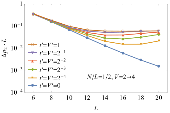
Figure 4: The log plot of $\Delta p_{2}\cdot L$ as a function of $L$ for the one-dimensional hard-core boson model driven by the interaction quench $V=2\to 4$ with $\beta=0$ at half filling ($N/L=1/2$).

In Fig. 4, we plot $\Delta p_{2}\cdot L$ as a function of $L$ for the one-dimensional hard-core boson model (14) at half filling ($N/L=1/2$). By comparing with Fig. 2 (for the filling $N/L=1/3$), one can see that the results do not qualitatively change while the filling is changed. In both cases, $\Delta p_{2}$ shows different scaling behaviors between non-integrable and integrable models. For the integrable case ($t^{\prime}=V^{\prime}=0$), $\Delta p_{2}$ decays exponentially, $\Delta p_{2}\sim e^{-cL}$ with $c=0.36$. The value of $c$ is different from that for $N/L=1/3$ (shown in the main text), so that $c$ is a non-universal quantity. On the other hand, in the non-integrable cases ($t^{\prime}\neq 0$ or $V^{\prime}\neq 0$) the results in Fig. 4 suggests that $\Delta p_{2}$ decays algebraically as $\Delta p_{2}\sim L^{-\gamma}$ with $\gamma=1$. This supports our expectation that the non-integrable scaling behavior is universal, and does not depend on details of the system such as the filling.

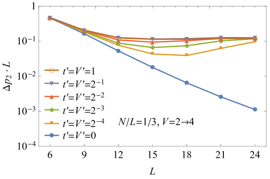
Figure 5: The log plot of $\Delta p_{2}\cdot L$ as a function of $L$ for the one-dimensional spinless fermion model (87) driven by the interaction quench $V=2\to 4$ with $\beta=0$ and $N/L=1/3$.

We also consider the one-dimensional spinless fermion model with nearest and next nearest neighbor hoppings and interactions Rigol (2009b); Santos and Rigol (2010),

$$\hat{H}(s) =-t\sum_{i}(f_{i}^{\dagger}f_{i+1}+\mbox{h.c.})+V(s)\sum_{i}n_{i}^{f}n_{i+1}^{f}-t^{\prime}\sum_{i}(f_{i}^{\dagger}f_{i+2}+\mbox{h.c.})+V^{\prime}\sum_{i}n_{i}^{f}n_{i+2}^{f},$$ (87)

where $f_{i}^{\dagger}$ creates a fermion at site $i$ and $n_{i}^{f}\equiv f_{i}^{\dagger}f_{i}$ is the fermion density operator. The model is known to be integrable when $t^{\prime}=V^{\prime}=0$ and non-integrable otherwise Rigol (2009b); Santos and Rigol (2010). In Fig. 5, we plot $\Delta p_{2}$ as a function of $L$ for the spinless fermion model. All the non-integrable cases flow into a single universal scaling behavior $\Delta p_{2}\sim L^{-\gamma}$ with the exponent $\gamma=1$, which is identical to that for the boson model. On the other hand, the integrable case shows an exponential decay $\Delta p_{2}\sim e^{-cL}$ with $c=0.29$.

References

(1)
G. N. Bochkov and Y. E. Kuzovlev, Sov. Phys. JETP 45, 125
(1977).
Evans et al. (1993)
D. J. Evans,
E. G. D. Cohen,
and G. P.
Morriss, Phys. Rev. Lett.
71, 2401 (1993).
Gallavotti and Cohen (1995)
G. Gallavotti and
E. G. D. Cohen,
Phys. Rev. Lett. 74,
2694 (1995).
Jarzynski (1997)
C. Jarzynski,
Phys. Rev. Lett. 78,
2690 (1997).
Crooks (1999)
G. E. Crooks,
Phys. Rev. E 60,
2721 (1999).
Esposito et al. (2009)
M. Esposito,
U. Harbola, and
S. Mukamel,
Rev. Mod. Phys. 81,
1665 (2009).
Campisi et al. (2011)
M. Campisi,
P. Hänggi, and
P. Talkner,
Rev. Mod. Phys. 83,
771 (2011).
Callen and Welton (1951)
H. B. Callen and
T. A. Welton,
Phys. Rev. 83,
34 (1951).
Kubo (1957)
R. Kubo, J.
Phys. Soc. Jpn. 12, 570
(1957).
Marconi et al. (2008)
U. M. B. Marconi,
A. Puglisi,
L. Rondoni, and
A. Vulpiani,
Phys. Rep. 461,
111 (2008).
Onsager (1931)
L. Onsager,
Phys. Rev. 37,
405 (1931).
Casimir (1945)
H. B. G. Casimir,
Rev. Mod. Phys. 17,
343 (1945).
(13)
J. Kurchan, arXiv:cond-mat/0007360.
(14)
H. Tasaki, arXiv:cond-mat/0009244.
(15)
M. G. A. Paris and J. Řeháček, eds., Quantum
State Estimation, Lect. Notes Phys. 649 (Springer, Heidelberg, 2004).
Lvovsky and Raymer (2009)
A. I. Lvovsky and
M. G. Raymer,
Rev. Mod. Phys. 81,
299 (2009).
Berry (1987)
M. V. Berry,
Proc. R. Soc. London Ser. A
413, 183 (1987).
Haake (2010)
F. Haake,
Quantum Signatures of Chaos
(Springer, New York,
2010).
Tsuji et al. (2018a)
N. Tsuji,
T. Shitara, and
M. Ueda,
Phys. Rev. E 97,
012101 (2018a).
Talkner et al. (2007)
P. Talkner,
E. Lutz, and
P. Hänggi,
Phys. Rev. E 75,
050102 (2007).
(21)
A. I. Larkin and Y. N. Ovchinnikov, Sov. Phys. JETP 28,
1200 (1969).
Swingle et al. (2016)
B. Swingle,
G. Bentsen,
M. Schleier-Smith,
and P. Hayden,
Phys. Rev. A 94,
040302 (2016).
Campisi and Goold (2017)
M. Campisi and
J. Goold,
Phys. Rev. E 95,
062127 (2017).
(24)
N. Y. Yao, F. Grusdt, B. Swingle, M. D. Lukin, D. M.
Stamper-Kurn, J. E. Moore, and E. Demler, arXiv:1607.01801.
Zhu et al. (2016)
G. Zhu,
M. Hafezi, and
T. Grover,
Phys. Rev. A 94,
062329 (2016).
Tsuji et al. (2017)
N. Tsuji,
P. Werner, and
M. Ueda,
Phys. Rev. A 95,
011601(R) (2017).
Yunger Halpern (2017)
N. Yunger Halpern,
Phys. Rev. A 95,
012120 (2017).
Yunger Halpern
et al. (2018)
N. Yunger Halpern,
B. Swingle, and
J. Dressel,
Phys. Rev. A 97,
042105 (2018).