Cooling of the rotation of a nanodiamond via the interaction with the electron spin of the contained NV-center

Abstract

We propose a way to cool the rotation of a nanodiamond, which contains a NV-center and is levitated by an optical tweezer. Following the rotation of the particle, the NV-center electron spin experiences varying external fields and so leads to spin-rotation coupling. By optically pumping the electrons from a higher energy level to a lower level, the rotation energy is dissipated. We give the analytical result for the damping torque exerted on the nanodiamond, and evaluate the final cooling temperature by the fluctuation-dissipation theorem. It’s shown that the quantum regime of the rotation can be reached with our scheme.

I Introduction

Since the seminal experiments of Ashkin in 1970 ashkin1 , the techniques of optical trapping and manipulation have developed rapidly over the past decades and stimulated remarkable advances in various fields of physics ashkin2 . In atomic physics, these techniques have greatly enhanced the ability to manipulate single atoms, leading to the experimental discovery of Bose-Einstein condensation wieman ; ketterle , the implementation of atom interferometry cronin and quantum simulations of condensed-matter systems with cold atoms bloch . More recently, optical manipulation has also been applied to larger objects such as micromirrors, cantilevers and dielectric nanoparticles to control the mechanical degrees of freedom vahala ; girvin1 ; favero ; genes1 ; kiesel ; schwab ; roels ; raizen , with the purposes of quantum information processing tian ; rips ; barz , ultrasensitive sensing geraci1 ; geraci2 ; du ; zhao and studying quantum-classical boundaries poot ; chen , etc. Theories regarding the cooling of center-of-mass (c.m.) motion were proposed zwerger ; zoller2 ; cirac1 ; cirac2 , and the quantum ground state cooling of a mechanical oscillator was realized experimentally cleland ; chan . Besides, the interaction between the rotation of a nano-body and the light has also been investigated cirac3 ; shi ; hoang . It is suggested that angular trapping and cooling of a dielectric can be achieved using multiple Laguerre-Gaussian cavity mode. The frequency of torsional vibration can be $1$ order of magnitude higher than the c.m. frequency hoang , which is promising for ground state cooling. Aside from being used for fundamental purposes, optically nanoparticle can also serve as ultrasensitive torque balance kim ; wu .

Recently, the coupling between the motion of a nanodiamond and the NV-center electron spin has attracted many research interests xu ; rabl ; arcizet ; lukin ; yin . The NV-center spin experiences varying external field following the motion of the nanodiamond, thus induces interaction between the spin and the mechanical motion, either translational or torsional. In this paper we propose a cooling scheme based on the spin-rotation coupling, the mechanism of which is similar to that of atomic laser cooling cohen1 ; cohen2 . A nanodiamond that contains a NV-center is levitated by an optical tweezer, hence its motion is confined. By applying external fields, the energy levels of NV-center are altered and left with an effective two-level system. In the course of rotation, the electrons in the higher level are optically pumped to the lower level, resulting in the dissipation of rotating energy of the nanodiamond, and thus achieves the effect of cooling. This paper is organized as folllowing: in Section I we outline the setup of the system and give a qualitative explanation of the cooling mechanism; Section II contains the calculation of the electronic state of the NV-center and the torque exerted on the nanodiamond; Based on these results, the cooling effect is analyzed in Section III; Finally we make conclusion in Section IV.

I.1 Setup of the system

We want to cool the rotation of a diamond nanoparticle that contains a NV-center. Firstly, the center of mass motion and rotation of the particle should be confined, which can be achieved by an optical tweezer. We consider a spheroid shaped nanoparticle with semi-major axis $a$ and semi-minor axis $b$ placed in a linearly polarized optical tweezer. If the size of the spheroid is much smaller than the wavelength of the laser, the electrostatic approximation can be used to describe the light-matter interaction. In a laser field with $Z$ polarization, the potential energy of the nanoparticle is:

$$U=-\frac{1}{2}\sum_{i}\alpha_{i}E_{i}^{2}=-\frac{1}{2}\alpha_{x}E^{2}-\frac{1}{2}(\alpha_{z}-\alpha_{x})E^{2}\cos^{2}\beta$$ (1)

where $\alpha_{x}$ and $\alpha_{z}$ are the polarizibilities along the principal axes, $E$ is the electric field strength of the laser and $\beta$ is the nutation angle of the nanoparticle (Fig.1). The electric field at the laser waist is determined by: $\varepsilon_{0}E^{2}=\frac{2P}{\pi cw^{2}}$ , where $P$ is the laser power, $c$ is the light speed, and $w$ is the waist. To give an estimation of the potential, we take $P=100mW$, $\pi w^{2}=2\mu m^{2}$, $a=40nm$, $b=20nm$, $\varepsilon_{r}=5.7$ (the dielectric constant of diamond), then the depth of the trap is

$$U(\beta=\frac{\pi}{2})-U(\beta=0)\simeq 5.6\times 10^{-21}J\equiv k_{B}T_{0}$$ (2)

with $T_{0}\simeq 400K$. At a temperature $T$, the nutation of the nanoparticle is confined in a range $[0,\beta_{m}]$, where $\beta_{m}$ is roughly determined by $k_{B}T_{0}(1-\cos^{2}\beta_{m})=\frac{1}{2}k_{B}T$, e.g., for $T=5K$, $\beta_{m}\simeq 4.5^{\circ}$.

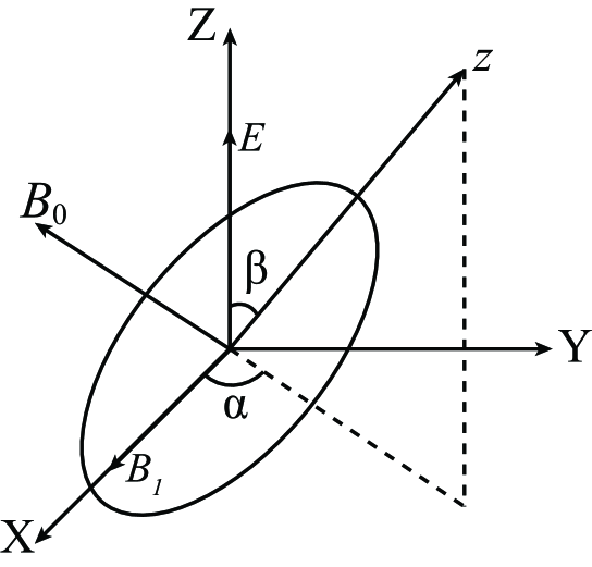
Figure 1: An ellipsoid rotates in external fields. $XYZ$ is the lab frame, $z$ is the major axis of the ellipsoid. $B_{0}$ is a static magnetic field that lies in the $XZ$ plane and has an angle $45^{\circ}$ to the $X$ axis. There is also a laser field $E$ along the $Z$ axis and an oscillating magnetic field $B_{1}\cos\omega t$ along the $X$ axis.

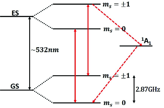
Figure 2: Electronic structure of the NV-center. GS is the ground state configuration and ES is the excited state configuration, each contains three sublevels $m_{s}=0,\pm 1$. A $532nm$ laser beam pumps the electrons in the $m_{s}=\pm 1$ states in the GS to $m_{s}=0$ state.

Now that the trap is produced, the cooling shall be achieved through interactions between the NV center and external fields. The electronic states of NV center are illustrated in Fig.2, where $GS$ is the ground state configuration and $ES$ is the excited state configuration, each contains three spin sublevels with magnetic quantum number $m_{s}=0,\pm 1$. The sublevels in ground state have a zero-field splitting $D=2.87GHz$ between the states $|0\rangle$ and $|\pm 1\rangle$. Our cooling scheme borrows the idea from atomic cooling proposed by Cohen-Tannoudji et al  cohen1 . First, a static magnetic field $\mathbf{B}_{0}$ (Fig.1) is applied to modulate the energies of states $|\pm 1\rangle$ when the quantization axis of the NV center (which is the $z$ axis) rotates. This is analogous to the modulation of the light-shifted energies for a moving atom. Second, another laser beam with $532nm$ wavelength is required to pump the electrons from $|\pm\rangle 1$ to $|0\rangle$ (Fig.2). The pumping process includes spontaneous emissions to an intermediate state and then to the $|0\rangle$ state, which causes dissipation of energy. Finally we need a microwave field $\mathbf{B}_{1}$ to induce transitions between $|0\rangle$ and $|\pm 1\rangle$, since otherwise all the electrons shall be pumped to $|0\rangle$ which is insensitive to external fields.

Now one may have a qualitative understanding of the cooling mechanism. If the frequency of the microwave field is $\omega$, the effective energies of states $|\pm 1\rangle$ are: $\delta_{\pm}=D-\omega\mp\gamma\mathbf{B}_{0}\cdot\hat{z}$, where $\hat{z}$ is the unit vector along $z$ direction. Since the rotation of the spheroid is confined by the optical trap, a suitable choice of $\omega$ and $\mathbf{B}_{0}$ makes that $\delta_{+}\ll\delta_{-}$ and the ground state reduces to a two level system with $m_{s}=0,1$. In the course of rotation, the electrons in level $|1\rangle$ are pumped to $|0\rangle$, and since the state of this system doesn’t follow the rotation adiabatically, as long as $\delta_{+}>0$ the energy is continuously dissipated and a friction force is produced, otherwise the system absorbs more energy from the $532nm$ laser than it loses in the spontaneous emissions. So to make sure the force is always frictional, the rotation angle must be confined to a range in which $\delta_{+}>0$. In the following we give the details of the calculation, which will confirm the above analysis.

I.2 Calculation of the torque

In the lab frame, the Hamiltonian describing the ground state configuration of the NV-center is:

$$H=DS_{z}^{2}-\gamma(\mathbf{B}_{0}+\mathbf{B}_{1}\cos\omega t)\cdot\mathbf{S}$$ (3)

where $S_{z}$ is the $z$ component of the spin-1 operator. It relates to the spin operators in $XYZ$ frame as: $S_{z}=\mathbf{S}\cdot\hat{z}=S_{X}\sin\beta\cos\alpha+S_{Y}\sin\beta\sin\alpha+S_{Z}\cos\beta$. For a rotating nanoparticle, $\alpha,\beta$ and also $S_{z}$ are time dependent in the lab frame, making the calculations difficult. So it’s better to move to the rotating frame, in which:

$$H^{\prime} = R^{\dagger}HR-iR^{\dagger}\frac{\partial R}{\partial t}=DS_{Z}^{2}-\gamma(\mathbf{B}_{0}+\mathbf{B}_{1}\cos\omega t)\cdot R^{\dagger}\mathbf{S}R$$ (4)

$$= DS_{Z}^{2}-\gamma(\mathbf{B}_{0}+\mathbf{B}_{1}\cos\omega t)\cdot R^{\dagger}\mathbf{S}R-\dot{\alpha}(S_{Z}\cos\beta-S_{X}\sin\beta)-\dot{\beta}S_{Y}$$

where $R=e^{-i\alpha S_{Z}}e^{-i\beta S_{Y}}$ is the rotating operator. Physically, such transformation is analogous to the unitary transformation made in the rotating wave approximation. In our setup, $\mathbf{B}_{0}$ is in the $XZ$ plane with an angle $45^{\circ}$ to the $X$ axis ($\mathbf{B}_{0}$ cannot be in the $Z$ direction. The reason for this will be shown later), and $\mathbf{B}_{1}$ points to the $X$ direction. This Hamiltonian is still time dependent due to the existence of microwave field $\mathbf{B_{1}}$, so we apply a second unitary transformation: $U=e^{-i\omega tS_{z}^{2}}$, and make the rotating wave approximation, then it becomes:

$$H_{e}=(D-\omega)S_{Z}^{2}-\frac{1}{\sqrt{2}}\gamma B_{0}(\cos\alpha\sin\beta+\cos\beta)S_{Z}-\dot{\alpha}\cos\beta S_{Z}-\frac{1}{2}\gamma B_{1}\cos\alpha\cos\beta S_{X}+\frac{1}{2}\gamma B_{1}\sin\alpha S_{Y}$$ (5)

This Hamiltonian sets up the basis of our following calculations. The terms depending on $S_{Z}$ give the unperturbed energies of $|0\rangle$ and $|\pm 1\rangle$ , which are $E_{0}=0$ and $E_{\pm}=D-\omega\mp[\frac{1}{\sqrt{2}}\gamma B_{0}(\cos\alpha\sin\beta+\cos\beta)+\dot{\alpha}\cos\beta]$, respectively. As discussed before, by suitably choosing $\omega$ and $B_{0}$ we can make $E_{+}\ll E_{-}$ so that this system becomes effectively two-level. This Hamiltonian explicitly depends on the angles $\alpha$ and $\beta$, so the nanoparticle experiences a torque:

$$\langle M_{\alpha}\rangle=\langle-\frac{\partial H_{e}}{\partial\alpha}\rangle=-\frac{1}{2}\gamma B_{1}\sin\alpha\cos\beta\langle S_{x}\rangle-\frac{1}{2}\gamma B_{1}\cos\alpha\langle S_{y}\rangle$$

$$\langle M_{\beta}\rangle=\langle-\frac{\partial H_{e}}{\partial\beta}\rangle=\frac{1}{\sqrt{2}}\gamma B_{0}(\cos\alpha\cos\beta-\sin\beta)\langle S_{z}\rangle-\frac{1}{2}\gamma B_{1}\cos\alpha\sin\beta\langle S_{x}\rangle$$ (6)

where $\langle...\rangle$ means $Tr(\rho...)$ and $\rho$ is the density matrix describing the state of the NV-center. In our setup, the microwave field $B_{1}$ is much smaller than the static field $B_{0}$, so in the following we focus on $M_{\beta}$.

The evolution of $\rho$ is governed by the master equation: $\dot{\rho}=-i[H_{e},\rho]+\mathcal{D}(\rho)$, or, in the component form:

$$\dot{\rho}_{11} = -\frac{1}{\sqrt{2}}g_{2}(\rho_{01}+\rho_{10})+\frac{i}{\sqrt{2}}g_{1}(\rho_{01}-\rho_{10})-\Gamma\rho_{11}$$

$$\dot{\rho}_{01} = i(\delta_{+}-\dot{\alpha}\cos\beta){\rho}_{01}+\frac{i}{\sqrt{2}}g_{1}(\rho_{11}-\rho_{00})+\frac{1}{\sqrt{2}}g_{2}(\rho_{11}-\rho_{00})-\Gamma_{1}\rho_{01}$$ (7)

where we have introduced the notations $g_{1}=\frac{1}{2}\gamma B_{1}\cos\alpha\cos\beta$, $g_{2}=\frac{1}{2}\gamma B_{1}\sin\alpha$, $\delta_{+}=D-\omega-\frac{1}{\sqrt{2}}\gamma B_{0}(\cos\alpha\sin\beta+\cos\beta)$. $\Gamma$ and $\Gamma_{1}$ are decay rates for $\rho_{11}$ and $\rho_{01}$ respectively.

If the nanoparticle is at rest, i.e. $\dot{\alpha}=\dot{\beta}=0$, the steady state of the NV-center is obtained by putting $\dot{\rho}_{11}=\dot{\rho}_{01}=0$. We get the steady values: $\rho^{s}_{11}=\frac{1}{2+f_{0}}$, $\rho^{s}_{01}=\frac{(ig_{1}+g_{2})f_{0}}{\sqrt{2}(2+f_{0})(\Gamma_{1}-i\delta_{+})}$ with $f_{0}=\frac{\Gamma(\Gamma_{1}^{2}+\delta_{+}^{2})}{\Gamma_{1}(g_{1}^{2}+g_{2}^{2})}$. For a rotating nanoparticle, the steady state satisfies $\dot{\rho}=\dot{\alpha}\frac{\partial\rho}{\partial\alpha}+\dot{\beta}\frac{\partial\rho}{\partial\beta}$, and Eq. (I.2) can be solved order by order. Note that $\Gamma_{1}\gg\Gamma$ liu , so $\rho_{01}$ follows almost adiabatically with the evolution of $\rho_{11}$ cohen2 : $\rho_{01}=\frac{(ig_{1}+g_{2})(\rho_{11}-\rho_{00})}{\sqrt{2}(\Gamma_{1}-i\delta_{+})}$. Inserting this formula to the first equation of (I.2) we get:

$$\dot{\alpha}\frac{\partial\rho_{11}}{\partial\alpha}+\dot{\beta}\frac{\partial\rho_{11}}{\partial\beta}=-\frac{(2+f)\Gamma}{f}(\rho_{11}-p_{s})$$ (8)

where $f=\frac{\Gamma[\Gamma_{1}^{2}+(\delta_{+}-\dot{\alpha}\cos\beta)^{2}]}{\Gamma_{1}(g_{1}^{2}+g_{2}^{2})}$, $p_{s}=\frac{1}{2+f_{0}}$. Expanding $\rho_{11}=p_{s}+p^{(1)}+...$ and $\frac{(2+f)\Gamma}{f}=\frac{(2+f_{0})\Gamma}{f_{0}}+\dot{\alpha}A_{1}+...$, then to the first order of $\dot{\alpha},\dot{\beta}$:

$$\dot{\alpha}(\frac{\partial p_{s}}{\partial\alpha}-A_{1}p_{s})+\dot{\beta}\frac{\partial p_{s}}{\partial\beta}=-\frac{(2+f_{0})\Gamma}{f_{0}}p^{(1)}$$ (9)

Hence

$$p^{(1)}=-\frac{f_{0}}{\Gamma(2+f_{0})}\big{(}\frac{\partial p_{s}}{\partial\alpha}\dot{\alpha}-A_{1}p_{s}\dot{\alpha}+\frac{\partial p_{s}}{\partial\beta}\dot{\beta}\big{)}$$ (10)

And from Eq. (I.2):

$$\langle M_{\beta}\rangle\approx\frac{1}{\sqrt{2}}\gamma B_{0}(\cos\alpha\cos\beta-\sin\beta)\big{(}p_{s}-\frac{f_{0}}{\Gamma(2+f_{0})}\frac{\partial p_{s}}{\partial\alpha}\dot{\alpha}-\frac{f_{0}}{\Gamma(2+f_{0})}\frac{\partial p_{s}}{\partial\beta}\dot{\beta}\big{)}\equiv M_{\beta}^{0}-\kappa_{\alpha\beta}\dot{\alpha}-\kappa_{\beta}\dot{\beta}$$ (11)

where $M_{\beta}^{0}$ is the conservative force and:

$$\kappa_{\alpha\beta} = \frac{1}{\sqrt{2}}\gamma B_{0}(\cos\alpha\cos\beta-\sin\beta)\frac{f_{0}}{\Gamma(2+f_{0})}\frac{\partial p_{s}}{\partial\alpha}\simeq-\frac{(\gamma B_{0})^{2}\delta_{+}f_{0}}{\Gamma_{1}(g_{1}^{2}+g_{2}^{2})(2+f_{0})^{3}}\sin\alpha\sin\beta(\cos\alpha\cos\beta-\sin\beta)$$

$$\kappa_{\beta} = \frac{1}{\sqrt{2}}\gamma B_{0}(\cos\alpha\cos\beta-\sin\beta)\frac{f_{0}}{\Gamma(2+f_{0})}\frac{\partial p_{s}}{\partial\beta}\simeq[\gamma B_{0}(\cos\alpha\cos\beta-\sin\beta)]^{2}\frac{\delta_{+}f_{0}}{\Gamma_{1}(g_{1}^{2}+g_{2}^{2})(2+f_{0})^{3}}$$ (12)

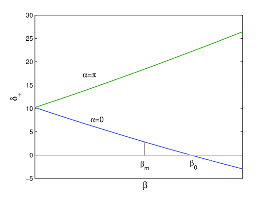
Figure 3: A sketch of $\delta_{+}$ as a function of $\beta$. The upper curve is for $\alpha=\pi$ and lower curve for $\alpha=0$, the value of $\delta_{+}$ for arbitrary $\alpha$ is between these two curves. At $\beta=\beta_{0}$ the lower curve crosses zero, so as long as $\beta\leq\beta_{m}<\beta_{0}$, $\delta_{+}$ is always positive.

The effect of $\kappa_{\alpha\beta}\dot{\alpha}$ will be discussed later and we focus on $\kappa_{\beta}\dot{\beta}$ now, which is a friction force as long as $\kappa_{\beta}>0$. From the above equation it’s seen that the sign of $\kappa_{\beta}$ is determined by $\delta_{+}$, which confirms the qualitative analysis in the previous section. As we mentioned before $\beta$ is confined by the optical trap in a range $[0,\beta_{m}]$, then by suitably choosing the frequency $\omega$ such that at a certain angle $\beta_{0}>\beta_{m}$ (but smaller than $45^{\circ}$), $D-\omega-\gamma B_{0}\cos(45^{\circ}-\beta_{0})=0$, one can make sure $\delta_{+}$ is always positive in the course of rotation (Fig.3).

The reason for that $\mathbf{B}_{0}$ can’t lie in the $Z$ axis is now clear. It’s seen $\kappa_{\beta}$ contains a factor $[B_{0}(\cos\alpha\cos\beta-\sin\beta)]^{2}$ which is proportional to $[\frac{d}{d\beta}(\mathbf{B}_{0}\cdot\hat{z})]^{2}$, then if $\mathbf{B}_{0}$ is in the $Z$ axis this will be $(B_{0}\sin\beta)^{2}$, making the friction force negligible for small $\beta$.

I.3 Analysis of cooling effect

We are now going to estimate the time scale over which the rotation is damped and the final cooling temperature. For small $\beta$, the Hamiltonian for the nanoparticle, which consists of the rotating energy and the potential of optical trap is:

$$H_{p}=\frac{I_{1}}{2}(\dot{\beta}^{2}+\dot{\alpha}^{2}\sin^{2}\beta)+\frac{I_{3}}{2}(\dot{\alpha}\cos\beta+\dot{\gamma})^{2}+U\simeq\frac{I_{1}}{2}\dot{\beta}^{2}+\frac{I_{3}}{2}(\dot{\alpha}+\dot{\gamma})^{2}+\frac{1}{2}(\alpha_{z}-\alpha_{x})E^{2}\beta^{2}$$ (13)

where a constant energy is omitted, and $I_{1}$, $I_{3}$ are moments of inertial about the $x$ and $z$ axes respectively. The torque exerted on the particle is produced by the optical trap as well as $M_{\beta}$, so the motion equation of $\beta$ is:

$$I_{1}\ddot{\beta}=-\frac{\partial U}{\partial\beta}+M_{\beta}=-\frac{\partial U}{\partial\beta}+M_{\beta}^{0}-\kappa_{\alpha\beta}\dot{\alpha}-\kappa_{\beta}\dot{\beta}+M^{\prime}_{\beta}$$ (14)

where $M^{\prime}_{\beta}=M_{\beta}-\langle M_{\beta}\rangle$ is the fluctuation of the torque. The time scale for damping is $t=\frac{I_{1}}{\kappa_{\beta}}$. In our case, $I_{1}=\frac{4\pi}{15}\rho ab^{2}(a^{2}+b^{2})$, where $\rho=3.5g/cm^{3}$ is the density of diamond, the other parameters are : $\Gamma=0.4\mu s^{-1}/2\pi$, $\Gamma_{1}=5\mu s^{-1}/2\pi$ and $\beta_{0}=9^{\circ}$. The dependence of $\kappa_{\beta}$ on $\beta$ is shown in Fig.4, where we take $\alpha=0$ and $\pi$ for examples. To give a rough estimation, taking $\kappa_{\beta}=500h$ for average, then $t\simeq 2.8\times 10^{-4}s$.

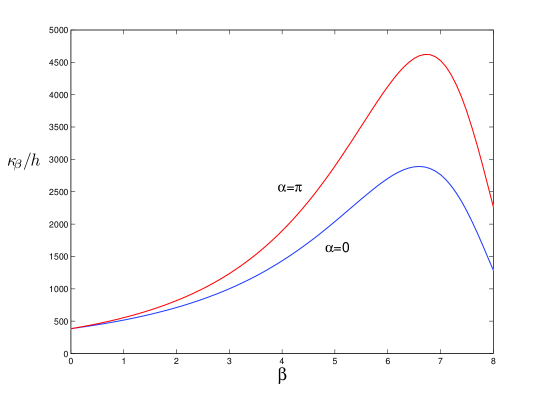
Figure 4: The $\beta$ dependence of $\kappa_{\beta}$ (in unit of the Planck constant $h$) with the following parameters: $\gamma B_{0}=2\pi\times 100MHz$, $\gamma B_{1}=2\pi MHz$, $\Gamma=0.4MHz$, $\Gamma_{1}=5MHz$ and $\beta_{0}=9^{\circ}$. The upper curve is for $\alpha=\pi$ and lower curve for $\alpha=0$.

The damping of $\dot{\alpha}$ is much slower than that of $\dot{\beta}$ since from Eq.(I.2) and (10), $M_{\alpha}\propto\gamma B_{1}$ , and is negligible compared to $M_{\beta}$ for $B_{1}\ll B_{0}$. So after some time of cooling, $\dot{\alpha}\gg\dot{\beta}$ and in a period $\tau$ that $\alpha$ changes from $0$ to $2\pi$, $\beta$ can be taken as a constant. Then the impulse of $\kappa_{\alpha\beta}\dot{\alpha}$ in such a period is:

$$\int_{0}^{\tau}\kappa_{\alpha\beta}\dot{\alpha}dt=\int_{0}^{2\pi}\kappa_{\alpha\beta}d\alpha=0$$ (15)

where the last equality results from $\kappa_{\alpha\beta}(\alpha)=-\kappa_{\alpha\beta}(2\pi-\alpha)$.

To estimate the final cooling temperature, we need to calculate the correlation function of the friction force. Let $G(t)=\langle S_{z}(t)S_{z}(0)\rangle-\langle S_{z}\rangle^{2}$, since $\langle S_{z}\rangle=p_{s}$, we have from the quantum regression theorem breuer that $\frac{dG}{dt}=-\frac{(2+f_{0})\Gamma}{f_{0}}G$ with initial condition $G(0)=p_{s}-p_{s}^{2}$. Then $G=G(0)\exp(-\frac{(2+f_{0})\Gamma}{f_{0}}t)$ and, from (I.2):

$$\langle M^{\prime}_{\beta}(t)M^{\prime}_{\beta}(0)\rangle=\frac{1}{2}[\gamma B_{0}(\cos\alpha\cos\beta-\sin\beta)]^{2}(p_{s}-p_{s}^{2})\exp(-\frac{(2+f_{0})\Gamma}{f}t)$$ (16)

Hence the momentum diffusion coefficient is:

$$D_{p}=\frac{1}{2}\int_{-\infty}^{\infty}\langle M^{\prime}_{\beta}(t)M^{\prime}_{\beta}(0)\rangle dt=\frac{1}{2}[\gamma B_{0}(\cos\alpha\cos\beta-\sin\beta)]^{2}(p_{s}-p_{s}^{2})\frac{f_{0}}{(2+f_{0})\Gamma}$$ (17)

where we have used the fact that for $t<0$, $\langle S_{z}(t)S_{z}(0)\rangle=\langle S_{z}(-t)S_{z}(0)\rangle$. So according to the fluctuation-dissipation theorem breuer , the temperature is:

$$k_{B}T_{f}=\frac{D_{p}}{\kappa_{\beta}}=\frac{(2+f_{0})^{2}(p_{s}-p_{s}^{2})(g_{1}^{2}+g_{2}^{2})\Gamma_{1}}{\delta_{+}\Gamma}=\frac{(1+f_{0})(g_{1}^{2}+g_{2}^{2})\Gamma_{1}}{\delta_{+}\Gamma}.$$ (18)

The angle $\beta$ will be about $0$ after a period of cooling, so we take $\beta=0$ in the above equation. Then $\delta_{+}=\gamma B_{0}[\cos(45^{\circ}-\beta_{0})-\cos 45^{\circ}]$ and $g_{1}^{2}+g_{2}^{2}=(\frac{1}{2}\gamma B_{1})^{2}$. Let’s consider the case $f_{0}=\frac{\Gamma(\Gamma_{1}^{2}+\delta_{+}^{2})}{\Gamma_{1}(g_{1}^{2}+g_{2}^{2})}\gg 1$, which can be fulfilled for $\gamma B_{0}\gg\gamma B_{1}$, then Eq. (19) is simplified as:

$$k_{B}T_{f}\simeq\frac{f_{0}(g_{1}^{2}+g_{2}^{2})\Gamma_{1}}{\delta_{+}\Gamma}=\frac{\Gamma_{1}^{2}+\delta_{+}^{2}}{\delta_{+}}$$ (19)

So the temperature reaches its minimum $2\Gamma_{1}/k_{B}$ at $\delta_{+}=\Gamma_{1}$. For $\Gamma_{1}=5MHz$, the lowest temperature is $T_{f}\simeq 0.6\times 10^{-4}K$. We want to see whether this temperature is low enough to reach the quantum regime. The Hamiltonian $H_{p}$ describes a harmonic oscillator with frequency $\omega_{0}=\sqrt{(\alpha_{z}-\alpha_{x})E^{2}/I_{1}}$, so the temperature for quantum regime is $\hbar\omega_{0}/k_{B}\sim 10^{-4}K$, which is of the same order of $T_{f}$.

II Conclusion

To conclude, we study the rotation cooling of a nanodiamond which contains a NV-center. Through the coupling between its rotation and the NV-center electron spin, the rotation energy is dissipated, which is similar to the atomic laser cooling. By suitably choosing the parameters of the system setup, the quantum regime can be reached. In our theory, the motion of nanoparticle is treated classically. However when the temperature is low enough, quantum effect must be taken into account. A full quantum mechanical approach is of our future interest.

Above we have assumed that there is only one NV-center in the nanodiamond. If the number of the NV-center is $n$, and if these NV-centers are uncorrelated, the damping coefficient $\kappa_{\beta}$ should be $n$ times the present one. However the final cooling temperature is unchanged since $D_{p}$ is also multiplied by a factor $n$.

III acknowledgements

This work is supported by Natural Science Foundation of Zhejiang Province LQ18A040003, NKBRP (973 Program) 2014CB848700 and No. 2016YFA0301201, NSFC No. 11534002 and NSAF U1530401, Science Challenge Project No.TZ2018003.

References

- (1) A. Ashkin, Phys. Rev. Lett. 24, 156 (1970).
- (2) M. H. Anderson, J. R. Ensher, M. R. Matthews, C. E. Wieman, and E. A. Cornell, Science 269, 198 (1995).
- (3) K. B. Davis, M.-O. Mewes, M. R. Andrews, N. J. van Druten, D. S. Durfee, D. M. Kurn, and W. Ketterle, Phys. Rev. Lett. 75, 3969 (1995).
- (4) A. Ashkin, Optical Trapping and Manipulation of Neutral Particles Using Lasers (World Scientific, Singapore, 2006).
- (5) A. D. Cronin, J. Schmiedmayer, and D. E. Pritchard, Rev. Mod. Phys. 81, 1051 (2009).
- (6) I. Bloch, J. Dalibard, and W. Zwerger, Rev. Mod. Phys. 80, 885 (2008).
- (7) P. Zoller et al., Eur. Phys. J. D 36, 203 (2005).
- (8) T. Kippenberg and K. Vahala, Science 321, 1172 (2008).
- (9) F. Marquardt and S. Girvin, Physics 2, 40 (2009).
- (10) I. Favero and K. Karrai, Nat. Photon. 3, 201 (2009).
- (11) C. Genes, A.Mari, D. Vitali, and P. Tombesi, Adv. At.Mol. Opt. Phys. 57, 33 (2009).
- (12) M. Aspelmeyer, S. Groblacher, K. Hammerer, and N. Kiesel, J. Opt. Soc. Am. B 27, A189 (2010).
- (13) M. Aspelmeyer and K. Schwab, New J. Phys. 10, 095001 (2008).
- (14) D. van Thourhout and J. Roels, Nat. Photon. 4, 211 (2010).
- (15) T. Li, S. Kheifets, and M. G. Raizen, Nat. Phys. 7, 527 (2011).
- (16) L. Tian, Phys. Rev. Lett. 108, 153604 (2012).
- (17) S. Rips and M. J. Hartmann, Phys. Rev. Lett. 110, 120503 (2013).
- (18) S. Barzanjeh, S. Guha, C. Weedbrook, D. Vitali, J. H. Shapiro, and S. Pirandola, Phys. Rev. Lett. 114, 080503 (2015)
- (19) A. A. Geraci, S. B. Papp, and J. Kitching, Phys. Rev. Lett. bf 105, 101101 (2010).
- (20) A. Arvanitaki and A. A. Geraci, Phys. Rev. Lett. 110, 071105 (2013).
- (21) P. Huang, P. Wang, J. Zhou, Z. Wang, C. Ju, Z. Wang, Y. Shen, C. Duan, and J. Du, Phys. Rev. Lett. 110, 227202 (2013).
- (22) N. Zhao and Z. Yin, Phys. Rev. A 90, 042118 (2014).
- (23) M. Poot and H. S. J. van der Zant, Physics Reports 511, 273 (2012).
- (24) Y. Chen, Journal of Physics B: Atomic, Molecular and Optical Physics 46, 104001 (2013).
- (25) I. Wilson-Rae, N. Nooshi, W. Zwerger, and T.J. Kippenberg, Phys. Rev. Lett. 99, 093901 (2007).
- (26) D. E. Chang, C. A. Regal, S. B. Papp, D. J. Wilson, O. Painter, H. J. Kimble, and P. Zoller, Proc. Natl. Acad. Sci. USA 107, 1005 (2010).
- (27) O. Romero-Isart, A. C. Pflanzer, M. L. Juan, R. Quidant, N. Kiesel, M. Aspelmeyer and J. I. Cirac, Phys. Rev. A 83, 013803 (2011).
- (28) A. C. Pflanzer, O. Romero-Isart and J. Ignacio Cirac, Phys. Rev. A 86, 013802 (2012).
- (29) A. D. O Connell, M. Hofheinz, M. Ansmann, R. C. Bialczak, M. Lenander, E. Lucero, M. Neeley, D. Sank, H. Wang, and M. Weides, J. Wenner, John M. Martinis, and A. N. Cleland, Nature 464, 697 (2010).
- (30) J. Chan, T. P. M. Alegre, A. H. Safavi-Naeini, J. T. Hill, A. Krause, S. Gr oblacher, M. Aspelmeyer, O, Painter, Nature, 478, 89 (2011).
- (31) O. Romero-Isart, M. L. Juan, R. Quidant, and J. I. Cirac, New J. Phys. 12, 033015 (2010).
- (32) H. Shi and M. Bhattacharya, J. Mod. Opt. 60, 382 (2013).
- (33) T. M. Hoang, Y. Ma, J. Ahn, J. Bang, F. Robicheaux, Z. Yin, and T. Li, Phys. Rev. Lett. 117, 123604 (2016).
- (34) P. H. Kim, C. Doolin, B.D. Hauer, A.J. MacDonald, M.R. Freeman, P.E. Barclay, and J.P. Davis, Appl. Phys. Lett. 102, 053102 (2013).
- (35) M. Wu, A.C. Hryciw, C. Healey, D.P. Lake, H. Jayakumar, M.R. Freeman, J.P. Davis, and P.E. Barclay, Phys. Rev. X 4, 021052 (2014).
- (36) Z. Y. Xu, Y. M. Hu, W. L. Yang, M. Feng, and J. F. Du, Phys. Rev. A 80, 022335 (2009).
- (37) P. Rabl, S. J. Kolkowitz, F. H.L. Koppens, J. G.E. Harris, P. Zoller, and M. D. Lukin, Nat. Phys. 6, 602 (2010).
- (38) O. Arcizet, V. Jacques, A. Siria, P. Poncharal, P. Vincent, and S. Seidelin, Nat. Phys. 7, 879 (2011).
- (39) S. Kolkowitz, A. C. Bleszynski Jayich, Q. P. Unterreithmeier, S. D. Bennett, P. Rabl, J. G. E. Harris, and M. D. Lukin, Science 335, 1603 (2012).
- (40) Y. Ma, T. M. Hoang, M. Gong, T. Li, and Z. Yin, Phys. Rev. A 96 023827 (2017).
- (41) J. Dalibard and C. Cohen-Tannoudji, S. Reynaud, J. Phys. B. 17, 4577 (1984).
- (42) L. Jin, M. Pfender, N. Aslam, P. Neumann, S. Yang, J. Wrachtrup and R. B. Liu, Nat. Comm. 6, 8251 (2015).
- (43) J. Dalibard and C. Cohen-Tannoudji, J. Opt. Soc. Am. B. 6, 2023 (1989).
- (44) H. P. Breuer, F. Petruccione, The Theory of Open Quantum Systems (Oxford University Press, 2002).
- (45) A. N. Volkov, Fluid Dyn. 44, 141 (2009)