Internal instabilities in magnetized jets

Abstract

We carry out an extensive linear stability analysis of magnetized cylindrical jets in a global framework. Foregoing the commonly invoked force-free limit, we focus on the small-scale, internal instabilities triggered in regions of the jet dominated by a toroidal magnetic field, with a weak vertical field and finite thermal pressure gradient. Such regions are likely to occur far from the jet source and boundaries, and are potential sites of magnetic energy dissipation that is essential to explain the particle acceleration and radiation observed from astrophysical jets. We validate the local stability analysis of Begelman by verifying that the eigenfunctions of the most unstable modes are radially localized. This finding allows us to propose a generic stability criterion in the presence of a weak vertical field. A stronger vertical field with a radial gradient complicates the stability criterion, due to the competition between the destabilizing thermal pressure gradient and stabilizing magnetic pressure gradients. Nevertheless, we argue that the jet interiors generically should be subject to rapidly growing, small-scale instabilities, capable of producing current sheets that lead to dissipation. We identify some new instabilities, not predicted by the local analysis, which are sensitive to the background radial profiles but have smaller growth rates than the local instabilities, and discuss the relevance of our work to the findings of recent numerical jet simulations.

1 Introduction

Astrophysical jets are bright, collimated and fast moving outflows that emanate from a wide variety of systems including young stellar objects (YSOs), active galactic nuclei (AGN), microquasars and gamma ray bursts (GRBs). Depending upon the source, these jets can be relativistic (e.g. AGN, microquasars, GRBs) or non-relativistic (e.g. YSOs). They traverse distances much larger than their initial radius, which is typically the size of their source, all the while maintaining a large-scale coherent structure. For instance, the jets from YSOs traverse $\lesssim$ 1pc, which is $\sim 10^{5}-10^{7}$ times the size of the central star, and those from AGN traverse $\gtrsim 10^{6}$ pc, which is $\sim 10^{9}$ times the size of the central supermassive black hole (see e.g. de Gouveia Dal Pino 2005; Beskin 2010 for an observational overview). Magnetic fields are believed to play an important role in governing the structure, dynamics and origin of these jets (e.g. Blandford & Znajek 1977). In spite of the differences in their environments and scales, the jets display very similar overall properties, not all of which are well understood. One of the major open areas of inquiry in this field is the question of jet stability (see e.g. Hardee 2011, 2013 for reviews on this subject).

It has been long known from basic plasma physics theory and laboratory experiments that cylindrical, magnetized plasmas are unstable to various kinds of instabilities (see e.g. Bateman 1978; Freidberg 1982, especially in the context of controlled fusion in tokamaks). In the case of a jet, these instabilities can be either kinetically or magnetohydrodynamically driven. The Kelvin-Helmholtz instability epitomizes the former category, and arises mainly due to the velocity shear created by the bulk motion of the jet with respect to the ambient medium (see Hardee 2013). The latter category is sub-classified as (see e.g. Longaretti 2008): (i) current-driven instabilities, which are driven by the current parallel ($j_{\parallel}$) to the total magnetic field ${\bf B}$ and are most easily studied in the context of cold, pressureless jets; and (ii) pressure-driven instabilities, which are driven by the gradient of the background plasma pressure and the electric current perpendicular ($j_{\bot}$) to ${\bf B}$. The curvature of the magnetic field lines plays an important role in confining the plasma in this case, and instability occurs when the destabilizing plasma pressure gradient is strong enough to push the plasma out of this curvature. If both components of the current are present, along with a finite plasma pressure gradient, then the instabilities will be of a mixed nature (see e.g. Striani et al., 2016). It can be roughly shown that pressure-driven effects dominate if $B_{z}\ll B_{\phi}$, which yields $j_{\bot}>j_{\parallel}$, and current-driven effects dominate if $B_{z}\gtrsim B_{\phi}$, which yields $j_{\bot}<j_{\parallel}$, where $B_{\phi}$ and $B_{z}$ are the toroidal and vertical magnetic fields, respectively (see e.g. Bonanno & Urpin 2011b). The two most commonly studied magnetohydrodynamic (MHD) instabilities in magnetized plasmas are the $m=0$ pinch mode and the $m=1$ kink mode, where $m$ is the azimuthal wavenumber. The former leads to a pinching distortion of the jet and triggers the so-called “sausage instability,” while the latter induces helical perturbations giving rise to the “kink instability” (see e.g. Hardee, 1979).

Depending on the lengthscales at which they operate, the above instabilities can be further classified as internal or external. Internal instabilities are small-scale modes compared to the jet radius, which are confined deep within the jet interior as the perturbations have no displacement at the jet boundaries. By definition these induce local changes (in morphology and energetics) without destroying the jet as a whole. External instabilities, on the other hand, are large-scale modes of the order of the jet radius, such that the perturbations have a non-zero displacement at the jet boundaries. These can potentially disrupt the whole jet. For instance, the external kink instability can bend and wiggle the entire jet off-axis, the external pinch instability can constrict the jet radius at various heights, and the Kelvin-Helmholtz instability due to the velocity shear at the jet surface can lead to mixing and interaction with the ambient medium.

The classical approach to understanding instabilities in jets is to perform a linear stability analysis of the ideal MHD equations. Many studies have been carried out using this approach, while invoking different magnetic field profiles, boundary conditions (impenetrable, free, outflow, etc.), methods of solution and physical assumptions (inclusion/exclusion of rotation, velocity shear, plasma pressure, etc.). Most of the analyses, however, have been carried out under the force-free assumption, where the system is magnetically dominated and the effect of plasma pressure is neglected. These include both non-relativistic (Appl, 1996; Appl et al., 2000) and relativistic (Istomin & Pariev, 1996; Lyubarskii, 1999; Tomimatsu et al., 2001; Narayan et al., 2009) analyses. The key developments in the linear stability analysis of cylindrical, relativistic, rotating and force-free jets can be summarized as follows. Istomin & Pariev (1996) showed that stability is achieved if $B_{z}$ is radially constant, while Lyubarskii (1999) showed that a $B_{z}$ decreasing radially outward induces instability. Tomimatsu et al. (2001), however, found a completely different criterion governed by the angular velocity of the magnetic field lines. Narayan et al. (2009) studied the effect of poloidal field curvature along with rigid rotation, with the aim of establishing a link between the various stability criteria. They found that their criterion is a generalization of the Kruskal-Shafranov stability criterion (which, however, does not account for rotation) for the $m=1$ kink mode (most relevant for tokamaks, e.g. Freidberg, 1982), which states that instability ensues when $B_{\phi}/B_{z}<2\pi R_{l}/L$, where $L$ is the length of the plasma column and $R_{l}$ its cylindrical radius. Recent numerical investigations in this context have been carried out by Mizuno et al. (2012); Bodo et al. (2013); Mizuno et al. (2014); Bodo et al. (2016); Sobacchi et al. (2017) and Sobacchi & Lyubarsky (2018). Begelman (1998, hereafter B98) was the first to consider the effect of the plasma pressure gradient balancing the magnetic gradients in a regime dominated by toroidal magnetic field (later works accounting for the plasma pressure include Baty & Keppens 2002; Bonanno & Urpin 2011b; O’Neill et al. 2012; Nalewajko & Begelman 2012; Kim et al. 2015). He performed a local study of the linear properties of short-wavelength, internal instabilities, and proposed a corresponding stability criterion. One of our aims in this work is to compare and validate the solutions from B98’s purely local calculations with those from the linear eigenvalue analysis in our global framework.

With the advancement of computational resources, numerical simulations of both non-relativistic and relativistic jets are now possible. These simulations are either local, where a small section of the 3D jet that is comoving with the bulk flow is modeled using periodic boundary conditions along the jet axis (Mizuno et al., 2009; O’Neill et al., 2012; Mizuno et al., 2012; Porth & Komissarov, 2015); semi-global, where a pre-existing jet is simulated in a non-periodic computational domain to better study the spatial development of various instabilities (Mizuno et al., 2014; Singh et al., 2016); or fully global, where the whole 3D jet is simulated starting from its injection/launch to large-scale propagation (Moll, 2009; McKinney & Blandford, 2009; Mignone et al., 2010; Bromberg & Tchekhovskoy, 2016). Numerical simulations are important in order to study the non-linear evolution and saturation of both the internal and external instabilities, as well as to visualize the morphological changes brought about by them in order to compare with observations. However, they still have limitations, as the results may depend significantly on the numerical solvers employed, resolution, launching mechanisms, etc. (see e.g. O’Neill et al. 2012). Thus, linear analyses are still relevant and essential for interpreting the complex numerical results and for making useful predictions.

Stability is a fundamental issue for jet studies in two complementary ways. First, since we know observationally that astrophysical jets survive and propagate for large distances, we can infer that they are somehow stable to the external instabilities. Such stability may be achieved due to (1) the jet speed becoming sufficiently supersonic or relativistic that external modes are suppressed or do not have enough time to grow; (2) rapid sideways expansion of the jet that breaks causal connection across it; (3) the stabilizing influence of rotation and velocity shear; or (4) a high density contrast or other properties of the ambient medium that promote stability (see e.g. Hardee 2011 for a discussion and, also, McKinney & Blandford 2009; Porth & Komissarov 2015; Bromberg & Tchekhovskoy 2016). Second, some kind of internal instability is needed in order to explain several jet observations, although overall jet stability and coherence are still desirable. In spite of various different mechanisms proposed (see references in Bromberg & Tchekhovskoy 2016), there is significant debate over what is responsible for the multi-wavelength emission from relativistic jets in AGN, microquasars and GRBs. It has been shown that internal kink-type instabilities are capable of triggering the dissipation of magnetic energy into thermal energy and radiation (see e.g. Mizuno et al. 2011; Porth et al. 2014 in the context of pulsar wind nebulae, and Lyutikov & Blandford 2003; Bromberg & Tchekhovskoy 2016 in the context of GRBs). This most likely occurs due to the formation of thin current sheets at small scales that facilitate reconnection of oppositely directed magnetic field lines being pushed closer together (see e.g. Kagan et al., 2015, for a review) — as demonstrated by MHD simulations (e.g. Singh et al., 2016) as well as fully-kinetic particle-in-cell (PIC) simulations (e.g. Sironi et al., 2015). Also, 3D resistive MHD simulations have shown that magnetized plasma columns can become unstable to both pressure-driven and current driven instabilities, which lead to the fragmentation of current sheets into filaments, followed by magnetic reconnection at an enhanced rate (Striani et al., 2016). The local dissipation zones created by internal instabilities can also serve as sites for particle acceleration, which is required to explain the observed non-thermal synchrotron and inverse Compton emission from relativistic jets (Sikora et al., 2005). This idea has gained considerable support from test particle acceleration studies that have been carried out in magnetic reconnection domains inside relativistic jets (see e.g. de Gouveia Dal Pino & Kowal, 2015, for a review). More, recently, efficient particle acceleration has also been demonstrated in both reconnection and turbulence studies using PIC simulations, and the results are in general consistent with jet observations (see e.g. Petropoulou et al., 2016; Guo et al., 2016; Zhdankin et al., 2017; Werner et al., 2018, and references therein). Furthermore, internal pinch and kink instabilities together can explain the rich, small-scale radial structures observed in jets, such as equispaced emission knots, wiggles, etc. (de Gouveia Dal Pino, 2005; Hardee, 2013). A lot of work has been done in trying to understand what perpetuates large-scale jet integrity. However, a fundamental understanding of internal instabilities is equally important, in order to answer basic questions such as how jets radiate.

In this work, we perform a comprehensive study of the linear development of internal instabilities and the associated stability criteria, by solving the global eigenvalue problem for a cylindrical magnetized plasma. Most linear studies of internal instabilities are carried out either in the force-free limit and/or in conjunction with studies of large-scale external instabilities that require the presence of an ambient medium. In our work, we drop the force-free assumption, and focus exclusively on the internal instabilities that are confined deep within the jet interior. We primarily model regions having a dominant toroidal magnetic field, a sub-dominant vertical magnetic field and a non-zero thermal pressure gradient, which is more prone to trigger pressure-driven instabilities. Most of the magnetic energy dissipation is supposed to take place in such a regime, which is likely to occur significantly away from the jet source. Our work thus expands on B98’s local, analytical calculations by self-consistently including the effects of radial gradients, geometric and magnetic curvatures, and a more complex toroidal field (B98 considered a radial power-law). We find that the maximum growth rates of the unstable modes are in excellent accord with the local prediction. More importantly, the B98 instability criterion — which essentially states that when the vertical field is very weak, the thermal pressure gradient is sufficiently strong and $B_{\phi}$ falls slower than $1/r$, then the underlying region is unstable to both axisymmetric and higher-order non-axisymmetric modes — holds true even in a global framework. This validation implies that dissipation in the jet interior is likely dominated by myriad local instabilities, i.e. radially localized modes, which tend to occur at large vertical wavenumbers and have the highest growth rates. Thus, we predict that fast growing, internal instabilities will always be triggered inside a jet as long as the B98 instability criterion is met locally, irrespective of the exact nature of the background radial profiles. Note that once triggered, the instabilities should have enough time to grow before the jet fluid moves to a significant distance from the source. B98 showed that these instabilities have growth times of the order of Alfvén crossing times, which are short enough in a toroidal field dominated region to develop non-linearly. Since in this work we recover growth rates very similar to those predicted by B98, the same conclusion applies. Not surprisingly, we also identify some intrinsically global instabilities, whose characteristics differ somewhat from the local predictions. These usually occur at smaller vertical wavenumbers and have smaller growth rates than the local instabilities. We clarify here that both the local and global instabilities in this work refer to small-scale, internal instabilities. In our context, local implies that the instabilities are insensitive to the background radial curvature and gradients, whereas the global instabilities are sensitive to these factors (i.e. global here is not to be confused with large-scale, external instabilities that we do not talk about in this work). We additionally test the effect of introducing a stronger vertical field and corresponding radial gradient. Such conditions tend to introduce aforementioned current-driven effects, and the stability criterion becomes more complex due to the interplay between the thermal and magnetic pressure gradients. We also compare our results with recently performed numerical jet simulations, in order to obtain more insight into the workings of real jets.

This paper is organized as follows. In §2, we lay out the basic properties of the jet model we study, along with the assumptions invoked and the underlying linearized MHD equations governing the problem. In §3, we discuss previously carried out analytical stability analyses most relevant to our work. We recall the local dispersion relation and stability criterion proposed by B98, the local stability criterion of Suydam (1958) and the magnetic resonance condition, all of which shall be tested in our global framework. In §4, we describe the numerical set-up and normalization scheme used for our global eigenvalue analysis. In §5, we present the detailed global solutions for different background conditions appropriate for jet interiors, and compare them with the local predictions wherever applicable. In §6, we compare our results with those of existing 3D jet simulations, with the aim of better understanding what triggers as well as quenches internal instabilities in jets. We conclude in §7, by summarizing our main results and their implications for observed astrophysical jets.

2 Theory

The literature studying MHD instabilities in the context of astrophysical jets is vast and rather confusing. It is indeed a complex topic and only a glimpse of this is given in the Introduction. Keeping this in mind, in this section we outline the main rationale behind our jet model, justify our assumptions and lay out the basic equations underlying the problem.

2.1 Jet model and assumptions

We carry out a linear stability analysis for the following jet model:

• We assume the jet to have a cylindrical geometry ($r,\phi,z$), threaded by an axisymmetric magnetic field ${\bf B}=(0,B_{0\phi}(r),B_{0z}(r))$, which is often referred to as a screw-pinch in the plasma physics literature. Note that we are particularly interested in studying the internal instabilities that may arise in a toroidal magnetic field dominated regime, which are predominantly pressure-driven in nature. Such a region may arise due to the following reasons. For a non-relativistic jet, as it propagates away from the source along the $z$-axis, the poloidal field is expected to fall off faster ($\sim 1/r^{2}$) than the toroidal field ($\sim 1/r$) in the radial direction due to magnetic flux conservation during lateral expansion (Begelman et al., 1984). In a relativistic jet, a toroidally dominated region can arise if the outer flux surfaces diverge away from the jet core, as demonstrated by Begelman & Li (1994), which can further explain the puzzle behind converting Poynting flux into kinetic energy in a magnetically dominated jet. We shall also briefly discuss the effect of a stronger poloidal field, likely to occur near the jet core, that makes current-driven effects important.

• In a real jet, it is likely that the complex magnetic field structure, bulk motion and velocity gradients make it quite hard to distinguish between the various instabilities triggered except at suitable limits (Baty & Keppens, 2002). In this work, however, our goal is to isolate the internal instabilities to the extent possible. Our global framework thus comprises an annular region of a static jet bounded by rigid walls (see §4.1 for details), which eliminates contamination due to the Kelvin-Helmholtz instability as well as the external kink acting at the jet boundaries (the vertical direction is still assumed to be local). Note that our inner radial boundary does not extend all the way up to the $r=0$ singularity (i.e. we do not study the instabilities that may arise in the jet core itself). This restriction does not interfere with our objective of studying the internal instabilities or testing the local calculations. In fact, it allows us to solve the global eigenvalue problem more accurately, i.e. without making any assumptions about the asymptotic behavior of the eigenfunctions at small radii (e.g. Bodo et al. 2013; Kim et al. 2015).

• The more commonly invoked force-free equilibrium is quite restrictive and, hence, we invoke the presence of a non-zero, thermal pressure gradient in the jet that balances the magnetic forces (following B98). Also, as internal instabilities are triggered in the jet, they are likely to dissipate magnetic energy into thermal energy, which further enhances the role of such a thermal pressure gradient.

• We perform our analysis in the non-relativistic limit, and assume the jet to be non-rotating as well as static (i.e. the fluid velocity ${\bf v}=0$). In other words, we work in the jet fluid-frame for simplicity. Note that we also ignore the effect of a comoving, poloidal velocity shear that may be present in the jet interior (see e.g. Nalewajko & Begelman, 2012).

2.2 Basic equations

We model our jet by invoking the ideal, non-relativistic MHD equations describing a magnetized, compressible fluid:

$$\frac{\partial\rho}{\partial t}+\nabla\cdot(\rho\mathbf{v})=0~{},$$ (1)

$$\frac{\partial\mathbf{v}}{\partial t}+(\mathbf{v}\cdot\nabla)\mathbf{v}+\frac{1}{\rho}\nabla\left(P+\frac{\mathbf{B}^{2}}{8\pi}\right)-\frac{1}{4\pi\rho}(\mathbf{B}\cdot\nabla)\mathbf{B}=0~{},$$ (2)

$$\frac{\partial\mathbf{B}}{\partial t}-\nabla\times(\mathbf{v}\times\mathbf{B})=0~{},$$ (3)

$$\nabla\cdot{\mathbf{B}}=0~{}~{}~{}{\rm or}~{}~{}~{}{\mathbf{B}}=\nabla\times{\mathbf{A}}~{}.$$ (4)

where $\rho$ is the density, $P$ the plasma pressure and ${\bf A}$ the magnetic vector potential. We substitute equation (4) in equation (3) to obtain

$$\frac{\partial\mathbf{A}}{\partial t}-(\mathbf{v}\times\mathbf{B})=0~{},$$ (5)

which is a particularly useful form of the magnetic induction equation when solving for non-axisymmetric perturbations. Recall that ${\bf B}$ is invariant under the gauge transformation ${\bf A}\rightarrow{\bf A}+\nabla\psi$, where $\psi$ is any scalar function. We also define the pitch ${\cal P}$ of the magnetic field, often invoked during the stability analysis of magnetized jet columns:

$${\cal P}=r\frac{B_{z}}{B_{\phi}}~{}.$$ (6)

The magnetic configurations studied in this work involve a wide range of pitch parameters.

Note that the vertical equilibrium is trivial as we do not consider any vertical gradients of the background quantities. The radial equilibrium is derived from equation (2), which on assuming an isothermal equation of state $P_{0}(r)=\rho_{0}(r)c_{s}^{2}$ can be written as:

$$\partial_{r}\rho_{0}=-\frac{B_{0\phi}}{4\pi c_{s}^{2}}\left[\frac{B_{0\phi}}{r}+\partial_{r}B_{0\phi}\right]-\frac{B_{0z}}{4\pi c_{s}^{2}}\partial_{r}B_{0z}~{},$$ (7)

where $c_{s}$ is the sound speed and the subscript ‘0’ denotes unperturbed background variables (see Appendix A). Note that because of the isothermal approximation, the density and plasma pressure gradient are synonymous in this work. The complete set of linearized MHD equations, obtained by perturbing equations (1), (2), (4) and (5), is given in Appendix A.

3 Analytical stability analyses

In this work, we compare the outcome of our global analysis with the solutions from B98’s local dispersion relation, which was derived for a magnetized, relativistic, non-rotating, compressible, cylindrically symmetric plasma (see eq. 3.32 of B98). In this section, we present only the relevant equations and final expression for this dispersion relation, and refer the readers to B98 and Das et al. (2018) for a detailed derivation. We also discuss the stability criteria proposed by B98, Suydam (1958) and the magnetic resonance condition.

3.1 B98 local dispersion relation

B98 considered a toroidally dominated configuration, having a weak, uniform vertical field, $B_{0z}\ll B_{0\phi}$ and power-law toroidal field, $B_{0\phi}\propto r^{\alpha}$. The perturbed variables were assumed to have the form

$$\exp i(lr+m\phi+k_{z}z-\omega t)~{},$$ (8)

where $\omega$ is the modal frequency, $t$ the time, $l$, $m$ and $k_{z}$ the radial, azimuthal and vertical wavenumbers respectively. The above form of the perturbations corresponds to the short wavelength approximation, i.e. $lr,k_{z}r\gg 1$, where the amplitudes are treated as constant coefficients. Note that $m$ can take only integer values such that $m=0,1,2$ etc., of which the $m=0$ (pinch) and $m=1$ (kink) modes are of particular interest to jet stability as discussed in the Introduction (the $m=2$ mode causes elliptical distortions). $m$ can be positive or negative, which indicates the sense of the spatial twist of the non-axisymmetric mode.

Table 1: Summary of the parameters introduced in the local analysis of §3.1 and §3.2.

Parameters	Notes
$\{\tilde{k}_{z},\tilde{l}\}=r_{0}\{k_{z},l\}$	dimensionless wavenumbers
${\tilde{\omega}}=\frac{r_{0}}{c_{s}}\omega$	dimensionless modal frequency
$\eta=\tilde{k}_{z}\frac{B_{0z}}{B_{0\phi}}$
$v_{A\phi}=\frac{B_{0\phi}}{\sqrt{4\pi\rho_{0}}}$	toroidal Alfvén velocity
$v_{Az}=\frac{B_{0z}}{\sqrt{4\pi\rho_{0}}}$	vertical Alfvén velocity
$d=\frac{c_{s}^{2}}{v_{A\phi}^{2}}$
$\beta=\frac{2c_{s}^{2}}{v_{A\phi}^{2}+v_{Az}^{2}}\approx 2d$	plasma-beta for $v_{Az}\ll v_{A\phi}$
$\alpha=\frac{\partial\ln B_{0\phi}}{\partial\ln r}$

The radial equilibrium given by equation (7) for the case considered by B98 simplifies to

$$\partial_{r}\rho_{0}=-(1+\alpha)\frac{B_{0\phi}^{2}}{4\pi c_{s}^{2}r}~{}.$$ (9)

Finally, the non-relativistic version of the local dispersion relation obtained by B98 can be written as (also, see Appendix B of Das et al. 2018):

$$\frac{1}{2}\biggl{(}1+\frac{l^{2}}{k_{z}^{2}}\biggr{)}\biggl{(}1+\frac{v_{A\phi}^{2}}{c_{s}^{2}}\biggr{)}\omega^{4} -\biggl{[}\biggl{(}1+\frac{l^{2}}{k_{z}^{2}}\biggr{)}(m+\eta)^{2}\biggl{(}1+\frac{v_{A\phi}^{2}}{2c_{s}^{2}}\biggr{)}\frac{v_{A\phi}^{2}}{r^{2}}-\alpha\biggl{(}1+\frac{v_{A\phi}^{2}}{c_{s}^{2}}\biggr{)}\frac{v_{A\phi}^{2}}{r^{2}}+\biggl{(}1-\frac{v_{A\phi}^{2}}{c_{s}^{2}}\biggr{)}\frac{v_{A\phi}^{2}}{r^{2}}\biggr{]}\omega^{2}$$

$$+(m+\eta)^{2}\frac{v_{A\phi}^{2}}{r^{2}}\biggl{[}\frac{1}{2}\biggl{(}1+\frac{l^{2}}{k_{z}^{2}}\biggr{)}(m+\eta)^{2}\frac{v_{A\phi}^{2}}{r^{2}}-(1+\alpha)\frac{v_{A\phi}^{2}}{r^{2}}\biggr{]}=0~{},$$ (10)

where all the new variables are defined in Table 1. This is a fourth-degree dispersion relation in $\omega$, obtained after neglecting the fast magnetosonic modes for simplicity. To derive this relation we have assumed, following B98, that the plasma-$\beta\approx 2c_{s}^{2}/v_{A\phi}^{2}$, since $v_{A\phi}\gg v_{Az}$. Hence, $v_{Az}$ only appears in the dispersion relation through $\eta$. We non-dimensionalize this equation such that all lengths are scaled by the local radial coordinate $r_{0}$, all wavenumbers by $1/r_{0}$, all velocities by $c_{s}$, all frequencies by $c_{s}/r_{0}$ and all densities by the local background density $\rho_{0}$ at $r_{0}$; which reduces equation (10) to the dimensionless form (see Table 1 for the new notation):

$$\frac{1}{2}\biggl{(}1+\frac{l^{2}}{k_{z}^{2}}\biggr{)}d(1+d){\tilde{\omega}}^{4} -\biggl{[}\biggl{(}1+\frac{l^{2}}{k_{z}^{2}}\biggr{)}(m+\eta)^{2}(1+2d)-\alpha(1+d)+(d-1)\biggr{]}{\tilde{\omega}}^{2}$$

$$+(m+\eta)^{2}\biggl{[}\frac{1}{2}\biggl{(}1+\frac{l^{2}}{k_{z}^{2}}\biggr{)}(m+\eta)^{2}-(1+\alpha)\biggr{]}=0~{}.$$ (11)

3.2 B98 local stability criterion

B98 found that relativistic effects have little effect on the growth rate of the unstable modes and, hence, his findings are applicable in the non-relativistic formalism as well. Seeking unstable modes such that $\omega^{2}<0$ and $\omega_{I}>0$ (as per the convention in equation 8), B98 obtained a necessary and sufficient condition for instability to occur (see eq. 4.2 of B98) such that

$$\frac{\partial\ln B_{0\phi}}{\partial\ln r}\equiv\alpha>\frac{1}{2}(m+\eta)^{2}-1$$ (12)

or, equivalently, unstable modes exist for

$$0<(m+\eta)^{2}<2(1+\alpha)~{}.$$ (13)

The above inequality clearly indicates that $\alpha=-1$ is the case of marginal stability for all $m$ or, equivalently, any local patch of the jet in which $B_{0\phi}$ decreases faster than $1/r$ should be stable with respect to both axisymmetric and higher-order non-axisymmetric modes. From equation (12) we can also say that for a given $m$ and $\alpha>-1$, instability occurs in the range

$$-\sqrt{2(1+\alpha)}-m<\eta<\sqrt{2(1+\alpha)}-m$$ (14)

or

$$(-\sqrt{2(1+\alpha)}-m)\frac{B_{0\phi}}{B_{0z}}<\tilde{k}_{z}|_{\rm unst}<(\sqrt{2(1+\alpha)}-m)\frac{B_{0\phi}}{B_{0z}}~{}.$$ (15)

Apart from the above instability criterion, B98 made certain estimates from his analytical calculations, which we quote here in the non-relativistic limit. First, B98 showed that the fastest growing modes (i.e. the modes having the most negative $\omega^{2}$) occur in the limit $l^{2}/k_{z}^{2}\ll 1$. Thus, putting $l^{2}/k_{z}^{2}\approx 0$, followed by minimizing $\omega^{2}$ with respect to $(m+\eta)^{2}$ in the dispersion relation given by equation (11), one obtains:

$${\tilde{\omega}}^{2}_{\rm min}=-8d\biggl{[}\biggl{(}1-\frac{1+\alpha}{4d}\biggr{)}-\biggl{(}1-\frac{1+\alpha}{2d}\biggr{)}^{1/2}\biggr{]}~{},$$ (16)

which is equivalent to eq. 4.8 of B98, when the relativity parameter $e$ therein is assumed to be $e\ll 1$. Thus, the maximum growth rate of the system is given by:

$${\tilde{\omega}}_{g}|_{\rm max}=\sqrt{8d\biggl{[}\biggl{(}1-\frac{1+\alpha}{4d}\biggr{)}-\biggl{(}1-\frac{1+\alpha}{2d}\biggr{)}^{1/2}\biggr{]}}~{},$$ (17)

which occurs at

$$(m+\eta)^{2}_{\rm min}=1+\alpha+\frac{1}{2}(1+2d){\tilde{\omega}}^{2}_{\rm min}~{},$$ (18)

which in turn is equivalent to eq. 4.9 of B98 for $e\ll 1$. Alternatively, the vertical wavenumbers corresponding to the most unstable modes are given by

$$\tilde{k}_{z}|_{\rm max}=\biggl{(}\pm\sqrt{1+\alpha+\frac{1}{2}(1+2d){\tilde{\omega}}^{2}_{\rm min}}-m\biggr{)}\frac{B_{0\phi}}{B_{0z}}~{}.$$ (19)

We note from equation (17) that the maximum growth rate is independent of $m$, which is a characteristic of pressure-driven instabilities. This is in contrast with current-driven instabilities, whose maximum growth rate is inversely proportional to $m$ (e.g. Appl et al., 2000).

3.3 Magnetic resonance condition

For non-axisymmetric perturbations in a cylindrical plasma column having the form given by equation (8), the magnetic resonance condition is defined as ${\bf k\cdot B}=0$, where ${\bf k}$ is the wave-vector with components $(l,m,k_{z})$. Consequently, one can define a resonant surface $r=r_{\rm res}$, where this condition is satisfied such that

$$k_{z}B_{z}(r_{\rm res})+\frac{m}{r_{\rm res}}B_{\phi}=0~{}.$$ (20)

The restoring force due to the magnetic tension is supposed to be minimum at these surfaces, which are hence more likely to trigger instabilities (see e.g. Longaretti 2008). By studying the global eigenfunctions of the most unstable modes, we shall test whether the above condition influences the instabilities in this work (see §5).

3.4 Suydam’s local stability criterion

Suydam (1958) proposed a necessary condition for stability for the non-axisymmetric ($m\neq 0$) modes of a screw-pinch such that

$$\frac{r}{4}\biggl{(}\frac{1}{{\cal P}}\frac{d{\cal P}}{dr}\biggr{)}^{2}+\frac{8\pi}{B_{z}^{2}}\frac{dP}{dr}\geq 0~{},$$ (21)

where ${\cal P}$ is the magnetic pitch given by equation (6). Note that this criterion was derived from a variational energy principle, which states that an equilibrium is unstable if the radial displacement of a mode makes the change in potential energy negative. Furthermore, this is a local stability criterion as the displacement of the concerned ($m,k_{z}$) modes is assumed to be localized only about the magnetic resonance surface (see equation 20), for reasons cited in §3.3. The thermal pressure gradient (second term in the inequality 21) has a negative sign and is known to drive the system to instability. Thus, Suydam’s criterion basically states that the magnetic shear (first term in the inequality 21) must be strong enough to counteract this effect to maintain stability. We shall revisit the applicability of this criterion when discussing our global solutions in §5. We note that although Sudyam’s criterion is local, it conveys the crucial point that a competition between the thermal and magnetic pressure gradients plays an important role in determining the stability of the system.

4 Global Eigenvalue Analysis

4.1 Numerical Set-up

In order to construct global solutions from the linearized axisymmetric system of equations (54)-(62), we consider the jet to be extended in radius $r\in[R_{\rm in},R_{\rm out}]$, to account for the curvature terms. As mentioned before, since we are only interested in the internal instabilities characterizing the jet, we assume this domain to be located far from the influence of the ambient medium as well as from the central axis (i.e. $R_{\rm in}\neq 0$). We solve equations (54)-(62) as a linear eigenvalue problem using the pseudo-spectral code Dedalus (Burns et al., in preparation). The solutions are decomposed on a basis of Chebyshev polynomials along the radial grid and on a Fourier basis in the vertical direction such that the perturbed variables have a form

$$f(r)\exp i(k_{z}z+m\phi-\omega t)~{},$$ (22)

and the linear eigenvalue problem becomes

$${\cal M}(r){\bm{\xi}}(r)=\omega{\cal I}{\bm{\xi}}(r)~{},$$ (23)

where $\omega=\omega_{R}+i\omega_{I}$ is the complex eigenvalue; ${\cal I}$ the identity operator; ${\cal M}(r)$ the MHD linear differential operator and ${\bm{\xi}}(r)$ the eigenfunction constituted of the perturbed variables in the system. The growth rate of an unstable mode is given by $\omega_{I}>0$, whereas $\omega_{R}$ is an indicator of the overstability of the mode.

We impose rigid/impenetrable boundary conditions at our inner and outer jet boundaries, such that (also, see Das et al. 2018):

$$v_{1r}=0~{}~{}~{}{\rm at}~{}~{}~{}r=R_{\rm in},R_{\rm out}$$

$$\partial_{r}B_{1z}=0~{}~{}~{}{\rm at}~{}~{}~{}r=R_{\rm in},R_{\rm out}~{},$$ (24)

where the subscript ‘1’ indicates perturbed variables (see Appendix A). These 4 boundary conditions suffice for the case with the Weyl gauge, however, for the Coulomb gauge we additionally impose

$$A_{1r}=0~{}~{}~{}{\rm at}~{}~{}~{}r=R_{\rm in},R_{\rm out}$$ (25)

to close the system of equations. We also impose boundary conditions on the background pressure/density, which we shall describe in §5. We choose our fiducial resolution to be either $N_{r}=200$ or $256$, where $N_{r}$ is the number of radial grid points. The fiducial radial extent of the jet is set to be $r\in[1,5]R_{\rm in}$, unless otherwise mentioned.

4.2 Normalization scheme

Table 2: Summary of the parameters introduced in the global analysis of §4 and §5.

Parameters	Definitions
$r\equiv\frac{r}{R_{\rm in}}$	dimensionless radius
$k_{z}\equiv k_{z}R_{\rm in}$	dimensionless vertical wavenumber
$\rho\equiv\frac{\rho}{\rho_{\rm in}}$	dimensionless density
$\omega_{I,R}\equiv\omega_{I,R}\frac{R_{\rm in}}{c_{s}}$	dimensionless eigenvalues (I $\equiv$ imaginary; R $\equiv$ real)
$v_{1r,1\phi,1z}\equiv\frac{v_{1r,1\phi,1z}}{c_{s}}$	dimensionless perturbed velocities
$v_{A\phi,Az}\equiv\frac{B_{\phi},z}{\sqrt{4\pi\rho_{\rm in}}}\frac{1}{c_{s}}$	dimensionless background Alfvén velocities
$v_{A\phi 0,Az0}$	background Alfvén velocities at $r=R_{\rm in}$
$\alpha=\frac{\partial\ln v_{A\phi}}{\partial\ln r}$	dimensionless parameter in $v_{A\phi}$-PL models
$a_{1}$	dimensionless parameter in $v_{A\phi}$-Gen models
$\epsilon$	dimensionless parameter in $v_{Az}$-Var models; $\frac{dP}{dr}=\frac{\epsilon}{1-\epsilon}\frac{d}{dr}\biggl{(}\frac{B_{z}^{2}}{8\pi}\biggr{)}$

We nondimensionalize our linearized equations (54)-(62) for the global analysis by using quantities at the inner radial jet boundary $R_{\rm in}$ (unless otherwise mentioned). We scale all lengthscales by $R_{\rm in}$, all wavenumbers by $1/R_{\rm in}$, all velocities by the sound speed $c_{s}$, all frequencies by $c_{s}/R_{\rm in}$ and all densities by the inner radial density $\rho_{\rm in}$. In order to solve the linearized equations, we replace $\partial_{z}\rightarrow ik_{z}$ and $\partial_{t}\rightarrow-i\omega$, and define dimensionless perturbed Alfvén velocities as

$$v_{A1r,A1\phi,A1z}\equiv\frac{B_{1r,1\phi,1z}}{\sqrt{4\pi\rho_{\rm in}}}\biggl{(}\frac{1}{c_{s}}\biggr{)}~{},$$ (26)

dimensionless perturbed vector potential components as

$$A_{1r,\phi,z}\equiv\frac{A_{1r,\phi,z}}{\sqrt{4\pi\rho_{\rm in}}}\biggl{(}\frac{1}{c_{s}R_{\rm in}}\biggr{)}$$ (27)

and dimensionless background Alfvén velocities as

$$v_{A\phi,Az}\equiv\frac{B_{\phi,z}}{\sqrt{4\pi\rho_{\rm in}}}\biggl{(}\frac{1}{c_{s}}\biggr{)}~{}.$$ (28)

Note that from here onwards we will describe the magnetic field in terms of the definition given by equation (28) (also, see Table 2 for a summary of the definitions to be used for the global analysis). Finally, depending on the gauge condition imposed, we solve for the set of eigenfunctions ${\bm{\xi}}(r)|_{Weyl}=\{\rho_{1},v_{1r},v_{1\phi},v_{1z},v_{A1\phi},v_{A1z},A_{1r},A_{1\phi},A_{1z}\}$ or ${\bm{\xi}}(r)|_{Coulomb}=\{\rho_{1},v_{1r},v_{1\phi},v_{1z},v_{A1\phi},v_{A1z},A_{1r},A_{1\phi},A_{1z},\psi\}$.

5 Global Solutions

In this section, we present the results of our global stability analysis. We divide the results into three categories depending upon the transverse magnetic field profiles adopted for the jet interior. There is a lot of uncertainty regarding the nature of magnetic fields inside jets, which has led different groups to adopt a wide range of field prescriptions (see references in the Introduction). However, our analysis reveals certain fundamental properties of the internal instabilities, which stand out irrespective of the complex nature of the magnetic field imposed.

Table 3: Summary of runs for case $v_{A\phi}{\rm-PL-}v_{Az}{\rm-Cons}$ presented in §5.1.

$m$	$\alpha$	$v_{A\phi 0}$	$v_{Az0}/v_{A\phi 0}$	$N_{r}$	B.C.s imposed on $\rho(r)$	Other notes
$0,1,2$	$-0.3$	$0.926$	$0.005$	$256$	$\rho(1)=1$; $\rho(r\rightarrow\infty)=0$	Fiducial $\alpha<0$ model; $v_{A\phi 0}=\sqrt{\frac{-2\alpha}{(1+\alpha)}}$
$0$	$-0.1$	$0.6$	$0.008$	$300$	$\rho(1)=1$	$\rho>0$ $\forall$ $r\in[1,5]$
$0$	$-0.3$	$0.6$	$0.008$	$200$	$\rho(1)=1$	$\rho>0$ $\forall$ $r\in[1,5]$
$0$	$-0.7$	$0.6$	$0.008$	$200$	$\rho(1)=1$	$\rho>0$ $\forall$ $r\in[1,5]$
$0$	$-0.9$	$0.6$	$0.008$	$200$	$\rho(1)=1$	$\rho>0$ $\forall$ $r\in[1,5]$
$0$	$-0.5$	$0.2$	$0.025$	$300$	$\rho(1)=1$	$\rho>0$ $\forall$ $r\in[1,5]$
$0$	$-0.5$	$0.6$	$0.008$	$300$	$\rho(1)=1$	$\rho>0$ $\forall$ $r\in[1,5]$
$0$	$-0.5$	$1.0$	$0.005$	$200$	$\rho(1)=1$	$\rho>0$ $\forall$ $r\in[1,5]$
$0$	$-0.5$	$1.25$	$0.004$	$200$	$\rho(1)=1$	$\rho>0$ $\forall$ $r\in[1,5]$
$0$	$-0.5$	$1.5$	$0.003$	$300$	$\rho(1)=1$	$\rho>0$ $\forall$ $r\in[1,5]$
$1$	$-0.1$	$0.6$	$0.008$	$200$	$\rho(1)=1$	$\rho>0$ $\forall$ $r\in[1,5]$
$1$	$-0.25$	$0.6$	$0.008$	$200$	$\rho(1)=1$	$\rho>0$ $\forall$ $r\in[1,5]$
$1$	$-0.3$	$0.6$	$0.008$	$200$	$\rho(1)=1$	$\rho>0$ $\forall$ $r\in[1,5]$
$1$	$-0.4$	$0.6$	$0.008$	$200$	$\rho(1)=1$	$\rho>0$ $\forall$ $r\in[1,5]$
$1$	$-0.5$	$0.6$	$0.008$	$200$	$\rho(1)=1$	$\rho>0$ $\forall$ $r\in[1,5]$
$1$	$-0.6$	$0.6$	$0.008$	$200$	$\rho(1)=1$	$\rho>0$ $\forall$ $r\in[1,5]$
$1$	$-0.7$	$0.6$	$0.008$	$200$	$\rho(1)=1$	$\rho>0$ $\forall$ $r\in[1,5]$
$1$	$-0.9$	$0.6$	$0.008$	$200$	$\rho(1)=1$	$\rho>0$ $\forall$ $r\in[1,5]$
$1$	$-0.5$	$\sqrt{2}$	$0.005$	$256$	$\rho(1)=1$ $\rho(r\rightarrow\infty)=0$	Pressure equipartition; $v_{A\phi 0}=\sqrt{\frac{-2\alpha}{(1+\alpha)}}$
$1$	$-0.3$	$0.926$	$0.001$	$200$	$\rho(1)=1$; $\rho(r\rightarrow\infty)=0$
$1$	$-0.3$	$0.926$	$0.01$	$200$	$\rho(1)=1$; $\rho(r\rightarrow\infty)=0$
$1$	$-0.3$	$0.926$	$0.1$	$200$	$\rho(1)=1$; $\rho(r\rightarrow\infty)=0$
$1$	$-0.3$	$0.926$	$0.5$	$200$	$\rho(1)=1$; $\rho(r\rightarrow\infty)=0$
$1$	$-0.3$	$0.926$	$0.75$	$200$	$\rho(1)=1$; $\rho(r\rightarrow\infty)=0$
$1$	$-0.3$	$0.926$	$1.0$	$200$	$\rho(1)=1$; $\rho(r\rightarrow\infty)=0$
$1$	$-0.3$	$0.926$	$0.005$	$256$	$\rho(r\rightarrow\infty)=10$	constant density background
$1$	$-0.3$	$0.926$	$0.005$	$256$	$\rho(r\rightarrow\infty)=100$	constant density background

5.1 Results for a power-law toroidal field and constant vertical field: $v_{A\phi}{\rm-PL-}v_{Az}{\rm-Cons}$

We begin by choosing a power-law for the toroidal field, $v_{A\phi}=v_{A\phi 0}r^{\alpha}$, and a constant vertical field, $v_{Az}=v_{Az0}$, where $v_{A\phi 0,Az0}$ are the respective quantities at the inner jet radius ($r=1$). This case provides a direct comparison with the local analysis of B98 and allows us to test the validity of the stability criterion proposed therein. The magnetic pitch for this case follows from equation (6) such that

$${\cal P}=r^{1-\alpha}\frac{v_{Az0}}{v_{A\phi 0}}~{}.$$ (29)

Thus, the pitch is an increasing function of radius if $\alpha<1$, a decreasing function if $\alpha>1$ and a constant if $\alpha=1$. All the runs carried out for this case are summarized in Table 3.

The background density for this case is obtained by integrating equation (7). Keeping our normalization scheme in mind (see Table 2), this yields

$$\rho(r)=-\frac{(1+\alpha)v_{A\phi 0}^{2}}{2\alpha}r^{2\alpha}+\rho_{\rm cons}~{},$$ (30)

where $\rho_{\rm cons}$ is the integration constant. Now, in order to determine $\rho_{\rm cons}$, we impose the inner boundary condition

$$\rho=1~{}~{}{\rm at}~{}~{}r=1~{},$$ (31)

which yields

$$\rho(r)=1+\frac{(1+\alpha)v_{A\phi 0}^{2}}{2\alpha}(1-r^{2\alpha})~{}.$$ (32)

The plasma-beta can be written as

$$\beta=\frac{2\rho(r)}{v_{A\phi 0}^{2}r^{2\alpha}+v_{Az0}^{2}}~{}.$$ (33)

However, one needs to keep in mind that if $v_{A\phi 0}$ becomes too large, and/or $\alpha$ assumes a large positive value, then the density may become negative beyond a certain radius. This puts a restriction on the computational domain for certain parameter values. If $\alpha<0$ on the other hand, then an additional outer boundary condition can be imposed such that

$$\rho\rightarrow 0~{}~{}{\rm as}~{}~{}r\rightarrow\infty~{}.$$ (34)

The above condition sets $\rho_{\rm cons}=0$ and self-consistently assures $\rho>0$ throughout the domain, yielding

$$\rho(r)=r^{2\alpha}~{}~{}~{}{\rm and}~{}~{}~{}v_{A\phi 0}=\sqrt{\frac{-2\alpha}{(1+\alpha)}}~{}.$$ (35)

Furthermore, on assuming $v_{Az0}\ll v_{A\phi}$, equation (33) reduces to

$$\beta\approx-\frac{1+\alpha}{\alpha}={\rm~{}constant}~{}.$$ (36)

Our fiducial model corresponds to $\alpha=-0.3$, $v_{A\phi 0}=0.926$, $v_{Az0}=0.005$ and $\beta\approx 2.33$. For this model, we impose both conditions (31) and (34) on the background density. However, in this case, $v_{A\phi 0}$ depends on $\alpha$ and is no longer a free parameter (see equation 35). Thus, for some cases (e.g. when varying $\alpha$ for a given $v_{A\phi 0}$, when $\alpha>0$, etc.), we impose only the condition (31). We use $r\in[1,5]$ for all the cases listed in Table 3, which also assures $\rho>0$ throughout the domain. We shall now discuss the properties of the axisymmetric $m=0$, and the non-axisymmetric $m=1$ and $2$ modes, corresponding to the cases listed in Table 3, separately.

5.1.1 Axisymmetric $m=0$ modes

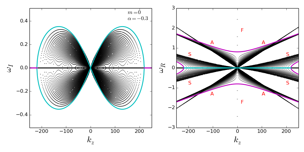
Figure 1: Global eigenvalue solutions for the fiducial $m=0$ case of $v_{A\phi}{\rm-PL-}v_{Az}{\rm-Cons}$, with $\alpha=-0.3$, $v_{A\phi 0}=0.926$ and $v_{Az}=v_{Az0}=0.005$. Left panel: The imaginary part $\omega_{I}$ of the modal frequency or, the growth rate, as a function of $k_{z}$. Right panel: The real part $\omega_{R}$ of the modal frequency as a function of $k_{z}$. The global eigenvalue solutions are shown in black. The cyan (unstable modes with $\omega_{I}>0$ and stable modes with $\omega_{I}<0$ in left panel, and the corresponding $\omega_{R}$ in right panel) and magenta (stable modes with $\omega_{I}=0$ in left panel and the corresponding $\omega_{R}$ in right panel) lines represent the solutions of the local dispersion relation, equation (11) with $l^{2}/k_{z}^{2}=0$. The letters F, S and A denote the fast, slow and Alfvén modes, respectively. The global problem is solved on a radial grid $r\in[1,5]$ with resolution $N_{r}$ = 256.

Figure 2: Normalized radial eigenfunction $v_{1r}$ for the most unstable modes as a function of radius $r$, for the case discussed in Figure 1. Top panels: $k_{z}>0$ modes. Bottom panels: $k_{z}<0$ counterparts of the respective top panels (see colored legends for $k_{z}$ values; note that $|k_{z}|$ increases from right to left in all panels). $\Delta r=r_{2}-r_{1}$ is the full-width at half maximum and $R_{\rm max}$ the radial peak location of the eigenfunctions. The radial axes in the right panels have been zoomed close to the inner boundary for clarity.

The main findings of this subsection, listed below, are summarized by Figures 1, 2 and 3:

1. The left panel of Figure 1 shows the imaginary part $\omega_{I}$ of the eigenvalues, or growth rate, as a function of the vertical wavenumber $k_{z}$ for the fiducial $\alpha=-0.3$ case (see Table 3). The right panel shows the real part $\omega_{R}$ of the corresponding eigenvalues. We also demarcate the fast magnetosonic, Alfvén and slow magnetosonic modes in the right panel, indicated by the letters F, A and S, respectively. Note that the total number of modes in the global problem is proportional to the radial resolution. The cyan ($\omega_{I}\neq 0$) and magenta ($\omega_{I}=0$) lines in this figure represent the corresponding local solutions predicted by the B98 dispersion relation, which are given by equation (11) with $l^{2}/k_{z}^{2}=0$.

   From the left panel of Figure 1, we see that the $m=0$ modes are symmetric about the $k_{z}$-axis (also, see equation 11), with $\omega_{I}=0$ at $k_{z}=0$. We also find that the $\omega_{I}>0$ cyan lines are in very good agreement with the growth rates of the most unstable modes of the global eigenvalue solution.

2. Some of the measurable quantities predicted by the local dispersion relation for this case are: the maximum growth rate $\omega_{g}|_{\rm max}\approx 0.35$ (see equation 17), the corresponding vertical wavenumbers $k_{z}|_{\rm max}\approx\pm 129$ (see equation 19) and the range of instability $-219\lesssim k_{z}|_{\rm unst}\lesssim 219$ (see relation 15). All the corresponding global quantities have comparable but slightly lower values as seen from Figure 1: $\omega_{g}|_{\rm max}\approx 0.33$, $k_{z}|_{\rm max}\approx\pm 124$ and $-206\lesssim k_{z}|_{\rm unst}\lesssim 206$. The growth rates of the most unstable modes in the range $0\leq k_{z}\lesssim 60$ are also slightly larger than the local prediction (see point (v) below).

3. On the right panel of Figure 1, note that the the cyan line indicates $\omega_{R}$ corresponding to the most unstable modes of the left panel ($\omega_{I}>0$), while the magenta lines indicate the $\omega_{R}$ corresponding to the stable modes ($\omega_{I}=0$ and $\omega_{I}<0$). From the global solutions we find that the most unstable modes are purely growing with zero phase velocity $\omega_{R}=0$, while the stable modes are purely oscillatory, corroborating the local predictions. In fact, the unstable modes appear to be destabilized slow modes. Note that the (stable) fast modes do not have a local counterpart as they are excluded from the local analysis (which yields a fourth-degree dispersion relation instead of sixth; see equation 11). A subtle difference between the local and global solutions is as follows: in the global solutions, as $k_{z}\rightarrow 0$, $\omega_{R}\rightarrow 0$ for all the Alfvén modes, unlike the local solutions, which have $\omega_{R}\neq 0$ for $k_{z}=0$. Also, for $|k_{z}|>160$ and $|\omega_{R}|>1.25$ (where the black lines intersect and then diverge away from the magenta lines), additional modes (possibly Alfvénic) appear in the global solutions that do not have a local counterpart.

4. We next discuss Figure 2, which shows the eigenfunction $v_{1r}$ as a function of radius for the most unstable mode at different $k_{z}$ corresponding to Figure 1. Note that the eigenfunctions are normalized with respect to their respective maximum amplitudes. Let us define two characteristics of the radial eigenfunctions, which will help us better understand the nature of the instabilities in this work. These are $\Delta r=r_{2}-r_{1}$, which is the full-width at half maximum of the eigenfunction, and $R_{\rm max}$, which gives the peak position of the eigenfunction as measured from the inner boundary $r=1$ (demonstrated with $k_{z}=8$ in the top left panel of Figure 2). Based on these, we can broadly classify any instability in the current work either as: (1) Local or (2) Global. A local instability has very narrow eigenfunctions (i.e. $\Delta r\lesssim 0.25$), which are highly concentrated (or localized) towards the inner boundary (i.e. $R_{\rm max}\rightarrow 1$). These properties indicate that the instability does not care about the radial variation of the background quantities like magnetic field and density and, hence, can be fully described by a local calculation (i.e. radially localized). A global instability, on the other hand, is affected by the background radial profiles and, hence, can only be captured in a global framework (i.e. radially extended). These can be of three kinds, having eigenfunctions that are: either wide and peak significantly away from the inner boundary (Global I, i.e. $\Delta r>0.25$ and $R_{\rm max}\nrightarrow 1$); or wide and peak towards the inner boundary (Global II, i.e. $\Delta r>0.25$ and $R_{\rm max}\rightarrow 1$); or narrow and peak significantly away from the inner boundary (Global III, i.e. $\Delta r\lesssim 0.25$ and $R_{\rm max}\nrightarrow 1$). Table 4 summarizes the characteristics of the various instabilities. We emphasize that although we distinguish between local and global instabilities here, they are both still internal, small-scale instabilities, which do not affect the large-scale properties of the jet.

   Table 4: Classification of the internal instabilities based on the properties of their radial eigenfunctions.

   Full-width at half maximum	Radial peak location	Type of instability
   $\Delta r\lesssim 0.25$	$R_{\rm max}\rightarrow 1$	Local
   $\Delta r>0.25$	$R_{\rm max}\nrightarrow 1$	Global I
   $\Delta r>0.25$	$R_{\rm max}\rightarrow 1$	Global II
   $\Delta r\lesssim 0.25$	$R_{\rm max}\nrightarrow 1$	Global III

   

   Figure 3: Growth rate $\omega_{I}$ as a function of $k_{z}$ for the $m=0$ case of $v_{A\phi}{\rm-PL-}v_{Az}{\rm-Cons}$ with $v_{Az0}=0.005$. Left panel: Cases when $v_{A\phi 0}=0.6$ is fixed and $\alpha$ is varied (see colored legends; note that $\alpha$ decreases from top to bottom). Right panel: Cases when $\alpha=-0.5$ is fixed and $v_{A\phi 0}$ is varied (see colored legends; note that $v_{A\phi 0}$ decreases from top to bottom). The dotted and dashed lines represent the global eigenvalue and local (equation 11) solutions respectively.

5. Keeping the above characteristics in mind, we can now look at the different eigenfunctions in Figure 2. The top left panel shows the eigenfunctions for $8\leq k_{z}\leq 55$, the top right for $85\leq k_{z}\leq 205$, the bottom left for $-55\leq k_{z}\leq-8$ and the bottom right for $-205\leq k_{z}\leq-85$ (the bottom panels thus representing the $k_{z}<0$ counterparts of the respective top panels). Note that the radial axes of the right panels of Figure 2 have been zoomed close to the inner boundary $r\in[1,1.5]$ for clarity, whereas the left panels show the full radial domain $r\in[1,5]$. We see that the eigenfunctions in the bottom panels are identical to their top-counterparts (except for a 180^∘ phase shift displayed by some), which again reflects the symmetry of the $m=0$ modes about the $k_{z}$-axis. The most unstable modes are found to be nodeless in general, across the entire range of unstable $k_{z}$. The modes shown in the left panels of Figure 2 have smaller $|k_{z}|$ than those in the right panel. They represent Global I and II instabilities. The eigenfunctions span a large radial extent, and as $|k_{z}|\rightarrow 0$, the modes seem to peak towards the outer boundary (Global I), gradually shifting towards the inner boundary as $|k_{z}|$ increases (Global II). This explains why the global solution in Figure 1 deviates from the local prediction as $k_{z}\rightarrow 0$. On the other hand, the larger $|k_{z}|$ modes in the right panels are Local instabilities, having narrow eigenfunctions that are highly localized close to the inner boundary. In general, the modes become more localized towards $r=1$ as $|k_{z}|$ increases.

6. In Figure 3, we study some interesting trends displayed by the $m=0$ modes. The left panel shows the evolution of the most unstable $m=0$ modes for a fixed $v_{A\phi 0}=0.6$ (and $\beta_{0}\approx 2/v_{A\phi 0}^{2}=5.55$), when $\alpha$ is varied. The dotted and dashed lines represent the global and local solutions respectively, which are in fairly good agreement. We find that as $\alpha$ decreases, the growth rates of the modes (in both local and global solutions) keep decreasing till they are completely stabilized at $\alpha=-1$, thus validating the B98 local stability criterion (see §3.2). The right panel of Figure 3, on the other hand, shows the corresponding evolution for a fixed $\alpha=-0.5$, when $v_{A\phi 0}$ is varied. We find that as $v_{A\phi 0}$ increases, the growth rates of the most unstable modes increase. We also see significant deviation from the local solution for $v_{A\phi 0}=1.5$ ($\beta_{0}=0.89$) at low $|k_{z}|$ values. This is possibly a consequence of the stronger toroidal field, which makes the radial curvature effects more important than the corresponding weaker field cases and, hence, necessitates a global analysis.

5.1.2 Non-axisymmetric $m=1$ modes

The main findings of this subsection, described below, are summarized by Figures 4-7:

1. 

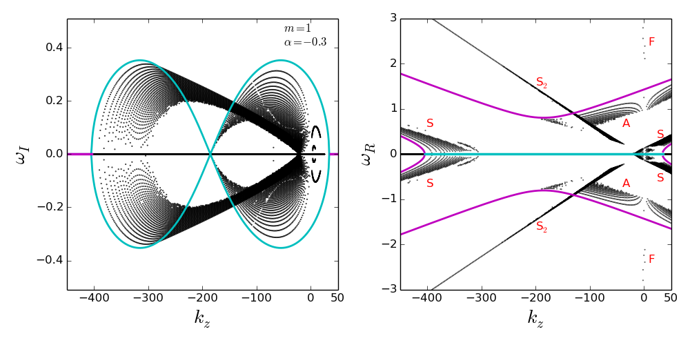
   Figure 4: Global eigenvalue solutions for the fiducial $m=1$ case of $v_{A\phi}{\rm-PL-}v_{Az}{\rm-Cons}$, with everything else the same as Figure 1. In the right panel, S₂ denotes a new branch of slow modes that appears in the global eigenvalue solutions.

2. Figure 4 is similar to Figure 1, except that it represents the fiducial $\alpha=-0.3$ case for the $m=1$ modes. All the symbols and colors have the same meaning in both figures. We note that the $m=1$ modes are no longer symmetric about the $k_{z}$-axis, as shown by both the local and global solutions. Also, non-axisymmetry seems to induce a somewhat greater deviation from the local prediction as compared to the axisymmetric case.

   First, we discuss the growth rates of the modes with $k_{z}>0$. From the left panel of Figure 4 we see that these modes have a much smaller growth rate than the local prediction. The local solution predicts a non-zero growth rate $\omega_{I}\approx 0.28$ at $k_{z}=0$ and instability in the range $0\leq k_{z}|_{\rm unst}\lesssim 34$. The growth rate in the global solution, on the other hand, has $\omega_{g}|_{\rm max}\approx 0.1$ at $k_{z}|_{\rm max}\approx 9$ and instability for $1\lesssim k_{z}|_{\rm unst}\lesssim 20$.

3. Next, we discuss the growth rates of the modes with $k_{z}<0$. Note that, as already mentioned at the beginning of §3.1, the sign of $m$ determines the direction of the helical twist. However, if $m$ is assumed to be positive, as we do in this work, then a negative $k_{z}$ in conjunction with a positive $m$ can be interpreted as the helical perturbation, or kink, twisting the magnetic field in a sense opposite to itself. On the other hand, a positive $k_{z}$ with a positive $m$ twists the magnetic field in the same direction as the kink. This is because the local dispersion relation (equation 10) is invariant under the transformation $(-m,k_{z})\rightarrow(m,-k_{z})$ or $(-m,\eta)\rightarrow(m,-\eta)$ .

   The local solution predicts two peaks with identical maximum growth rates $\omega_{g}|_{\rm max}\approx 0.35$ (see cyan lines in the left panel of Figure 4). The first instability peak occurs at $k_{z}|_{\rm max}\approx-55$ and the second at $k_{z}|_{\rm max}\approx-315$, with the instability in the range $-404\lesssim k_{z}|_{\rm unst}\leq 0$. The double-peaked structure is due to the local magnetic resonance occurring at $r=r_{\rm res}=1$ for $k_{z}|_{\rm res}=-mv_{A\phi 0}/v_{Az0}\approx-185$ (see equation 20), which segregates the two $k_{z}<0$ instability peaks. One can thus interpret the instabilities to be originating from $r_{\rm res}=1$ (see §3.3) in the local scenario. However, an important point to note is that magnetic resonance is an intrinsically global condition. Thus, in order to truly understand if it plays any role, we need to check if the unstable eigenfunctions have significant amplitude at the corresponding resonant radius. This can be only verified in a global framework, as demonstrated in point (vi) below.

   The global solution also exhibits two peaks in the growth rate, which are, however, not identical unlike the local solution (left panel of Figure 4). The peak values and $k_{z}$ locations differ slightly from the local values, matching more closely for the second peak: $\omega_{g}|_{\rm max}\approx 0.32$ at $k_{z}|_{\rm max}\approx-63$ and $\omega_{g}|_{\rm max}\approx 0.34$ at $k_{z}|_{\rm max}\approx-304$ and instability in the range $-392\lesssim k_{z}|_{\rm unst}\leq 0$. The behavior at $k_{z}\approx-185$, where local magnetic resonance is satisfied, is also very different. In the global solution, although the first instability peak stabilizes at $k_{z}\approx-185$, the second peak does not originate from $k_{z}\approx-185$, but from $k_{z}=0$. This leads to an interaction between the unstable modes in the global scenario, which appears as a band between the two instability peaks (these are slow-mode-slow-mode interactions).

   

   Figure 5: Normalized radial eigenfunction $v_{1r}$ for the most unstable modes as a function of radius $r$, for the case discussed in Figure 4 (see colored legends for $k_{z}$ values; note that $|k_{z}|$ increases from right to left in all panels). The green dashed vertical line, in the second panel from left, indicates the resonant radius $r_{\rm res}=2.86$ for $k_{z}=-135$ (green dashed curve), given by equation (20). Note that the radial range shown differs from panel to panel for clarity, although the global problem is solved on a grid $r\in[1,5]$.

4. On the right panel of Figure 4, we find that the most unstable modes have zero phase velocity ($\omega_{R}=0$) like the $m=0$ case, and are likely to be destabilized slow modes. For $k_{z}>0$, the local solutions seem to be tracing the slow and Alfven modes of the global solutions fairly well. For $k_{z}<0$, we see the appearance of possibly another branch of slow modes (marked as S₂) that does not have a local counterpart, which also seems to be interacting with the Alfvén modes.

   

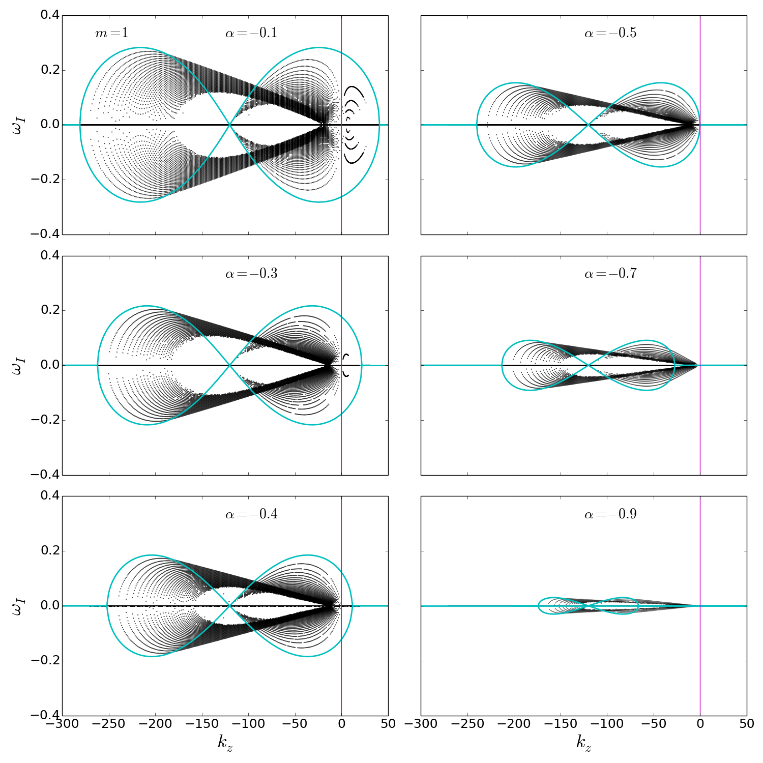
   Figure 6: Growth rate $\omega_{I}$ as a function of $k_{z}$ for the $m=1$ case of $v_{A\phi}{\rm-PL-}v_{Az}{\rm-Cons}$, when $v_{A\phi 0}=0.6$ and $v_{Az0}=0.005$ are fixed, and $\alpha$ is varied. The magenta vertical line indicates the $k_{z}=0$ line in each panel. The global eigenvalue solutions are shown in black. The cyan lines are the corresponding local solutions from the dispersion relation given by equation (11) with $l^{2}/k_{z}^{2}=0$.

5. For a detailed understanding of the nature of the $m=1$ instabilities, we need to look at the corresponding eigenfunctions. Figure 5 shows the eigenfunction $v_{1r}$ as a function of radius for the range of unstable $k_{z}$ corresponding to Figure 4. The eigenfunction shown here is that of the most unstable mode at a given $k_{z}$. Starting from left, the first panel shows the eigenfunctions for $3\leq k_{z}\leq 18$, the second for $-135\leq k_{z}\leq-10$, the third for $-250\leq k_{z}\leq-140$ and the last for $-390\leq k_{z}\leq-270$, plotted on radial axes, $r\in[1,5]$, $r\in[1,3]$, $r\in[1,3]$ and $r\in[1,1.2]$, respectively, for clarity. We now classify the instabilities according to Table 4.

   The first panel of Figure 5 shows that the eigenfunctions for $k_{z}>0$ represent Global I ($k_{z}<5$) and Global II ($5<k_{z}<18$) modes. This explains the deviation of the global solution from the local prediction in this $k_{z}$-range, as seen in the left panel of Figure 4. The decrease of $v_{A\phi}$ with $r$ suppresses the growth rate of the global $k_{z}>0$ modes compared to the local value.

   The modes with $k_{z}<0$ exhibit mixed behaviors. The second panel shows that the modes with $k_{z}\geq-45$ are Global II instabilities, which progress to becoming Local instabilities for $-135\leq k_{z}\leq-63$. This is reflected in the left panel of Figure 4, where we see that the global eigenvalues approach the local prediction (cyan line) as $k_{z}\rightarrow-135$.

   The eigenfunctions in the third panel represent Global III instabilities and are unique in the sense that they are shifted away from both the radial boundaries. These eigenfunctions represent the interaction between the two sets of $k_{z}<0$ instabilities mentioned in point (ii) above (also see left panel of Figure 4). As $k_{z}\rightarrow-250$, the eigenfunctions tend to get localized close to the inner boundary again.

   Finally, the eigenfunctions in the last panel represent Local instabilities, and hence the global eigenvalue solution for this range of $k_{z}$ matches well with the local prediction, as seen in the left panel of Figure 4. Overall, we find that the eigenfunctions become more localized towards $r=1$ as $|k_{z}|$ increases, similar to the $m=0$ case.

6. Figure 6 shows the effect of varying $\alpha$ on the growth rates of the $m=1$ modes, for a fixed $v_{A\phi 0}=0.6$ and $v_{Az0}=0.005$ (compare with the left panel of Figure 3 for the equivalent $m=0$ case). As $\alpha$ decreases, the growth rates of all the modes decrease for both the local and global solutions. The $k_{z}>0$ unstable modes stabilize first. In the global eigenvalue solution these modes stabilize at $\alpha=-0.4$, slightly higher than the local prediction of stabilization at $\alpha=-0.5$ (see equation 15). This is probably due to the fact that the $k_{z}>0$ modes are Global instabilities, as discussed above and, hence, they stabilize earlier due to the rapid fall in $v_{A\phi}$ with radius as $\alpha$ decreases. Nevertheless, we may still consider $\alpha=-0.5$ as an absolute stability criterion for the $k_{z}>0$ modes, when $m=1$. As $\alpha$ decreases beyond $-0.5$, instability exists only for $k_{z}<0$. We see that the onset of instabilities as per the local solution keeps shifting to lower $k_{z}$. The instabilities in the global solution also seem to pull away from $k_{z}=0$ slightly as $\alpha\rightarrow-1$, however at a much slower rate than the local solutions. The small $|k_{z}|$ modes thus correspond to Global instabilities (I or II; see point (iv) above), which deviate from the local prediction. Finally, at $\alpha=-1$ there is complete stabilization of all the $m=1$ modes, again validating B98’s local stability criterion.

7. We now discuss the resonant character of the $m=1$ modes from a global perspective. For the power-law profile in this section, the $m=1$ modes satisfying the magnetic resonance condition (equation 20) are given by $k_{z}=-v_{A\phi 0}r^{\alpha}/v_{Az0}$. Thus, for our fiducial domain $1\leq r\leq 5$, the most unstable modes with $-185\lesssim k_{z}\lesssim-114$ are supposed to be resonant and the ones outside this range are non-resonant. We now look at the eigenfunctions of these modes.

   Note that the most unstable modes in the range $-185\lesssim k_{z}\lesssim-140$, shown in the third panel of Figure 5, are the interacting slow modes mentioned in point (ii) above, and are unlikely to be resonant. The most unstable modes in the range $-135\lesssim k_{z}\lesssim-114$, shown in the second panel, could in principle be resonant. In order to verify this, we need to compare the the peak locations of these eigenfunctions with the corresponding resonant radius $r_{\rm res}$ from equation (20).

   Consider the example of $k_{z}=-135$ in the second panel of Figure 5. It is highly localized close to the inner boundary, peaking at $r\sim 1.02$, i.e. well inside the resonant surface for this mode at $r_{\rm res}=(-k_{z}v_{Az0}/v_{A\phi 0})^{1/\alpha}\sim 2.86$ (green dashed vertical line in second panel of Figure 5). Thus, the amplitude of the eigenfunction is effectively zero at $r_{\rm res}$, which implies that magnetic resonance is not actually triggering these modes. Note that the role of magnetic resonance might be sensitive to the background as well as boundary conditions. For example, Bodo et al. (2013) indeed found unstable modes that peak at the corresponding resonant radius in their stability analyses carried out for relativistic, force-free, pressureless jets with surface velocity shear. Alternatively, Kim et al. (2015) showed that the presence of a finite pressure dilutes the importance of the magnetic resonance condition in triggering instabilities.

8. With reference to the above discussion on magnetic resonance, we can further conclude that Suydam’s criterion is not applicable to check for instability in this case, as the unstable modes are not localized about $r_{\rm res}$ (see §3.4). We do, however, find an interesting result for $\alpha=-1$. The left hand side of the Suydam’s stability criterion (inequality 21) reduces, in our units and notation, to

   $$\frac{1}{4r}(1-\alpha)^{2}-\frac{2}{r}(1+\alpha)\frac{v_{A\phi}^{2}}{v_{Az}^{2}}~{},$$ (37)

   which is $\geq 0$ for $\alpha\leq-1$. This happens to be consistent with the stability condition for the $m=1$ modes established above (i.e. B98 stability criterion).

   

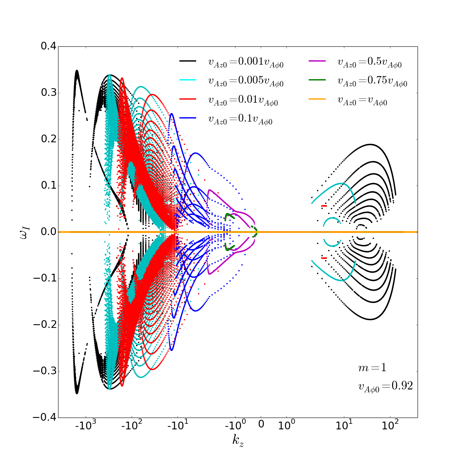
   Figure 7: Growth rate $\omega_{I}$ as a function of $k_{z}$ for the $m=1$ case of $v_{A\phi}{\rm-PL-}v_{Az}{\rm-Cons}$, when $v_{A\phi 0}=0.926$ and $\alpha=-0.3$ are fixed, and $v_{Az0}$ is varied (see colored legends; note that maximum growth rate decreases as $v_{Az0}$ increases). Only global eigenvalue solutions are shown in this figure. The $k_{z}$-axis is in log scale.

9. The $m=1$ instabilities are likely to be responsible for the dissipation of magnetic energy into thermal energy in the jet due to the formation of current sheets (as mentioned in the Introduction). This may lead to an enhanced background pressure, which in turn can affect the instabilities. In order to study this, we add a constant background pressure (which in our case corresponds to a constant density) to our fiducial model. We test two cases: $\rho_{\rm cons}=\rho(r\rightarrow\infty)=10$ and $\rho_{\rm cons}=\rho(r\rightarrow\infty)=100$ (see equation 30 and Table 3). Note that the above densities are normalized using the same inner density $\rho_{\rm in}$ as our fiducial model, i.e. when $\rho_{\rm cons}=\rho(r\rightarrow\infty)=0$, in order to maintain the same magnetic field profile for all three cases. We find that an enhancement in the background pressure leads to a suppression of the maximum growth rates, which can be roughly approximated as $\propto\omega_{\rm fidu}\rho_{\rm cons}^{-0.5}$, where $\omega_{\rm fidu}$ is the maximum growth rate of the fiducial case. However, the stability criteria remains unchanged, and we observe the same range of unstable $k_{z}$, as well as the same $k_{z\rm max}$, for all the cases. We also verified that even in the presence of an enhanced background pressure, the system gets stabilized as $\alpha\rightarrow-1$.

10. So far, we have restricted our discussion to the limit $v_{Az}\ll v_{A\phi}$ (see Introduction and §2.1 for the motivation behind this) and, hence, to predominantly pressure-driven instabilities. However, if the vertical field becomes strong enough, it can have a stabilizing effect by counteracting the hoop stress due to the toroidal field. Also, as mentioned towards the beginning of the Introduction, a stronger vertical field is likely to introduce current-driven effects, which may induce a change in the behavior of the instabilities.

    Figure 7 shows the growth rates of the $m=1$ modes as $v_{Az0}$ is increased with respect to $v_{A\phi 0}$ for our fiducial $\alpha=-0.3$ case (only global eigenvalue solutions are shown). For $0.001v_{A\phi 0}\leq v_{Az0}\leq 0.01v_{A\phi 0}$, the maximum growth rate of the $m=1$ modes remain fairly similar and this is the limit up to which the local calculations are valid. As $v_{Az0}$ increases further, we see that the maximum growth rate starts decreasing, although it is still appreciable for $v_{Az0}=0.1v_{A\phi 0}$. There is a sharp drop in the maximum growth rate for $v_{Az0}\geq 0.5v_{A\phi 0}$ and complete stabilization for $v_{Az0}=v_{A\phi 0}$, where the vertical field dominates over the toroidal field everywhere in the domain (since $v_{Az0}$ is a constant and $v_{A\phi 0}$ decreases with radius). Nevertheless, it has been pointed out that even a strong vertical field may lead to instability if $m$ is sufficiently high (see Bonanno & Urpin 2011a for a discussion). Note that when $v_{Az0}=0.1v_{A\phi 0}$, the $k_{z}>0$ modes stabilize for $\alpha=-0.3$ in contrast to the case shown in Figure 6 ($v_{Az0}=0.005v_{A\phi 0}$), where they stabilize for $\alpha=-0.4$. Thus, with an increase in the vertical field, the $k_{z}>0$ modes are marginally stabilized at higher $\alpha$. Similarly, there is complete stabilization for all $k_{z}$-modes at a higher value of $\alpha$, and $\alpha\leq-1$ reduces to a sufficient (and no longer necessary) stability criterion.

5.1.3 Non-axisymmetric $m=2$ modes

The main findings of this subsection, discussed below, are summarized by Figures 8 and 9:

1. Figure 8 is similar to Figures 1 and 4, with the same color-scheme and symbolization, except that it represents the $m=2$ modes. Like the $m=1$ modes, the $m=2$ modes are not symmetric about the $k_{z}$-axis. There is also significant deviation from the local prediction.

   First, we discuss the growth rates of the $m=2$ modes in the left panel of Figure 8. We see that there is no instability for $k_{z}>0$, as shown by both the local and global solutions. This is true for a wide range of $\alpha$, namely $\alpha\leq 1$, as seen from equation (15). The local solution predicts two peaks with the same maximum growth rate $\omega_{g}|_{\rm max}\approx 0.35$. From the cyan lines we see that the first instability peak occurs at $k_{z}|_{\rm max}\approx-240$ and the second at $k_{z}|_{\rm max}\approx-500$, with the instability occupying a total range $-590\lesssim k_{z}|_{\rm unst}\leq-151$. The local magnetic resonance corresponds to $k_{z}|_{\rm res}=-mv_{A\phi 0}/v_{Az0}\approx-370$ at $r=1$, which again separates the two peaks in the local solution.

   

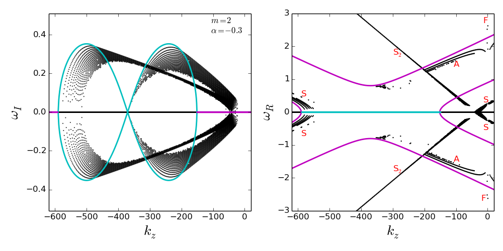
   Figure 8: Global eigenvalue solutions for the fiducial $m=2$ case of $v_{A\phi}{\rm-PL-}v_{Az}{\rm-Cons}$, with everything else same as Figures 1 and 4.

   The global solution also exhibits two peaks in the growth rate, which match fairly well with the local prediction (the first peak has a slightly smaller $\omega_{I}\approx 0.34$ than the second peak). However, the instability onsets at a much lower $|k_{z}|$ in the global solution, yielding a total range $-580\lesssim k_{z}|_{\rm unst}\leq-20$. Also, both the instability peaks originate from $k_{z}\approx-20$, contrary to the local solution.

   Examining the right panel of Figure 8, the global solutions have similar characteristics to the $m=1$ case (see right panel of Figure 4). The most unstable modes have zero phase velocity like both the $m=0$ and $m=1$ cases, and are likely to be destabilized slow modes. There is significant deviation from the local solutions, with a new branch of slow modes (marked S₂) appearing and interacting with the Alfvén modes, just like in the $m=1$ case.

   

   Figure 9: Normalized radial eigenfunction $v_{1r}$ for the most unstable modes as a function of radius $r$, for the case discussed in Figure 8 (see colored legends for $k_{z}$ values; note that $|k_{z}|$ increases from right to left in all panels). The red dashed vertical line, in the second panel from left, indicates the resonant radius $r_{\rm res}=1.91$ for $k_{z}=-305$ (red dashed curve), given by equation (20). Note that the radial axes has been plotted for different extents in the four panels for clarity, although the global problem is solved on a grid $r\in[1,5]$.

2. Figure 9 shows the eigenfunctions $v_{1r}$ for a range of unstable $k_{z}$. Note that we only plot the eigenfunction corresponding to the most unstable mode at a given $k_{z}$ to avoid confusion. Starting from left, the first panel shows the eigenfunctions for $-160\leq k_{z}\leq-25$, the second for $-305\leq k_{z}\leq-190$, the third for $-450\leq k_{z}\leq-310$ and the last for $-570\leq k_{z}\leq-487$, with different radial axes for clarity, namely, $r\in[1,5]$, $r\in[1,2]$, $r\in[1,1.8]$ and $r\in[1,1.1]$ respectively. We now classify the instabilities according to Table 4.

   From the first panel of Figure 9, we see that the eigenfunction for $k_{z}=-25$ peaks towards the outer boundary. We have verified that all modes in the range $-25<k_{z}<0$ exhibit a similar behavior and, hence, represent Global I instabilities. These then transform to Global III instabilities in the range $-160<k_{z}<-25$, which is an indication of slow-mode-slow-mode interaction. The eigenfunctions in the second panel clearly represent Local instabilities. The eigenfunctions in the third panel represent Global III instabilities, signifying the slow-mode-slow-mode interaction in the range $-450<k_{z}<-310$. The eigenfunctions in the last panel again represent Local instabilities. Note that there are two sets of interacting instabilities for $m=2$ (first and third panel of Figure 9), unlike the $m=1$ case, which has only one (third panel of Figure 5).

3. The $m=2$ modes satisfying the magnetic resonance condition (equation 20) are given by $k_{z}=-2v_{A\phi 0}r^{\alpha}/v_{Az0}$. Thus, for our fiducial domain $1\leq r\leq 5$, the modes with $-370\lesssim k_{z}\lesssim-228$ are supposed to be resonant. The most unstable modes in the range $-370\lesssim k_{z}\lesssim-310$ are interacting in nature and, hence, non-resonant (third panel of Figure 9). The modes in the range $-305\lesssim k_{z}\lesssim-228$, in the second panel, are supposed to be resonant, but they are localized far away from the corresponding resonant radii. Thus, again magnetic resonance does not play any role in triggering the $m=2$ instabilities. The inapplicability of Suydam’s criterion remains the same as for the $m=1$ case, since the inequality (21) holds true for all $m\neq 0$.

The global solutions yield very similar maximum growth rates for the $m=0,1,2$ cases studied in this section (see left panels of Figures 1, 4 and 8). This is in accordance with the local prediction for pressure-driven instabilities (see equation 17). Although not shown here, we have verified that the $m=2$ modes also get completely stabilized as $\alpha\rightarrow-1$. Physically this condition means that the destabilizing thermal pressure gradient vanishes when $\alpha=-1$ (see equation 9). Interestingly, the background equilibrium becomes force-free but not pressureless when $\alpha=-1$. Thus, $\alpha\leq-1$ can be interpreted as a global stability criterion for all axisymmetric and non-axisymmetric modes, for a nearly constant vertical field such that $v_{Az}\ll v_{A\phi}$. The reason the local B98 stability criterion holds true even for the global solutions is because the fastest growing modes are purely Local instabilities (occurring at large $|k_{z}|$) irrespective of $m$.

5.2 Results for a power-law toroidal field and varying vertical field: $v_{A\phi}{\rm-PL-}v_{Az}{\rm-Var}$

Table 5: Summary of runs for case $v_{A\phi}{\rm-PL-}v_{Az}{\rm-Var}$ with $\alpha=-0.3$ presented in §5.2.

$m$	$\epsilon$	$v_{A\phi 0}=\sqrt{\frac{-2\alpha}{\epsilon(1+\alpha)}}$	$v_{Az0}=\sqrt{\frac{2(1-\epsilon)}{\epsilon}}$	$v_{Az0}/v_{A\phi 0}$	$N_{r}$	B.C.s imposed on $\rho(r)$
$0$	$0.999$	$0.926$	$0.045$	$0.048$	200	$\rho(1)=1$; $\rho(r\rightarrow\infty)=0$
$0$	$0.99$	$0.930$	$0.142$	$0.153$	200	$\rho(1)=1$; $\rho(r\rightarrow\infty)=0$
$0$	$0.9$	$0.976$	$0.471$	$0.483$	200	$\rho(1)=1$; $\rho(r\rightarrow\infty)=0$
$0$	$0.8$	$1.035$	$0.707$	$0.683$	200	$\rho(1)=1$; $\rho(r\rightarrow\infty)=0$
$1$	$0.999$	$0.926$	$0.045$	$0.048$	256	$\rho(1)=1$; $\rho(r\rightarrow\infty)=0$
$1$	$0.99$	$0.930$	$0.142$	$0.153$	256	$\rho(1)=1$; $\rho(r\rightarrow\infty)=0$
$1$	$0.9$	$0.976$	$0.471$	$0.483$	256	$\rho(1)=1$; $\rho(r\rightarrow\infty)=0$
$1$	$0.8$	$1.035$	$0.707$	$0.683$	256	$\rho(1)=1$; $\rho(r\rightarrow\infty)=0$
$1$	$0.7$	$1.106$	$0.926$	$0.837$	200	$\rho(1)=1$; $\rho(r\rightarrow\infty)=0$
$1$	$0.4$	$1.464$	$1.732$	$1.18$	300	$\rho(1)=1$; $\rho(r\rightarrow\infty)=0$

In this section, we discuss the effect of a radially varying vertical field on the instabilities (for a power-law toroidal field). In order to do so, we make the following assumption about the relation between the thermal pressure gradient and the vertical field gradient:

$$\frac{d}{dr}\biggl{(}\frac{B_{z}^{2}}{8\pi}\biggr{)}=\biggl{(}\frac{1-\epsilon}{\epsilon}\biggr{)}\frac{dP}{dr}~{},$$ (38)

where $0<\epsilon<1$. Thus, a larger value of $\epsilon$ indicates a stronger thermal pressure gradient and vice versa. Note that equation (38) is an idealization and may not hold true inside a jet column. Nevertheless, this formalism helps us understand the basic contribution of a vertical field gradient towards the stability of the system.

Using the above equation and assuming $v_{A\phi}=v_{A\phi 0}r^{\alpha}$, with $\alpha<0$, we can integrate equation (7) to obtain the background density (or equivalently, thermal pressure) as a function of radius. We impose the boundary conditions (31) and (34) to obtain:

$$\rho(r)=r^{2\alpha}~{}~{}{\rm and}~{}~{}v_{Az}(r)=v_{Az0}r^{\alpha}~{},$$ (39)

such that

$$v_{Az0}=\sqrt{\frac{2(1-\epsilon)}{\epsilon}}~{}~{}{\rm and}~{}~{}v_{A\phi 0}=\sqrt{\frac{-2\alpha}{(1+\alpha)\epsilon}}~{}.$$ (40)

Note that we also assumed $v_{Az}\rightarrow 0$ as $r\rightarrow\infty$. The plasma-beta for this case is a constant with respect to radius (for a given $\alpha$ and $\epsilon$) such that

$$\beta=\frac{2}{(v_{A\phi 0}^{2}+v_{Az0}^{2})}=\frac{\epsilon(1+\alpha)}{1-\epsilon(1+\alpha)}~{}.$$ (41)

The magnetic pitch for this case can be written using equation (6) as

$${\cal P}=r\frac{v_{Az0}}{v_{A\phi 0}}=r\sqrt{\frac{(1-\epsilon)(1+\alpha)}{-\alpha}}~{},$$ (42)

which always increases with radius. We shall now study the effect of varying $\epsilon$ on the stability of the $m=0$ and $m=1$ modes for $\alpha=-0.3$. The cases are listed in Table 5. We use $r\in[1,5]$ for all cases.

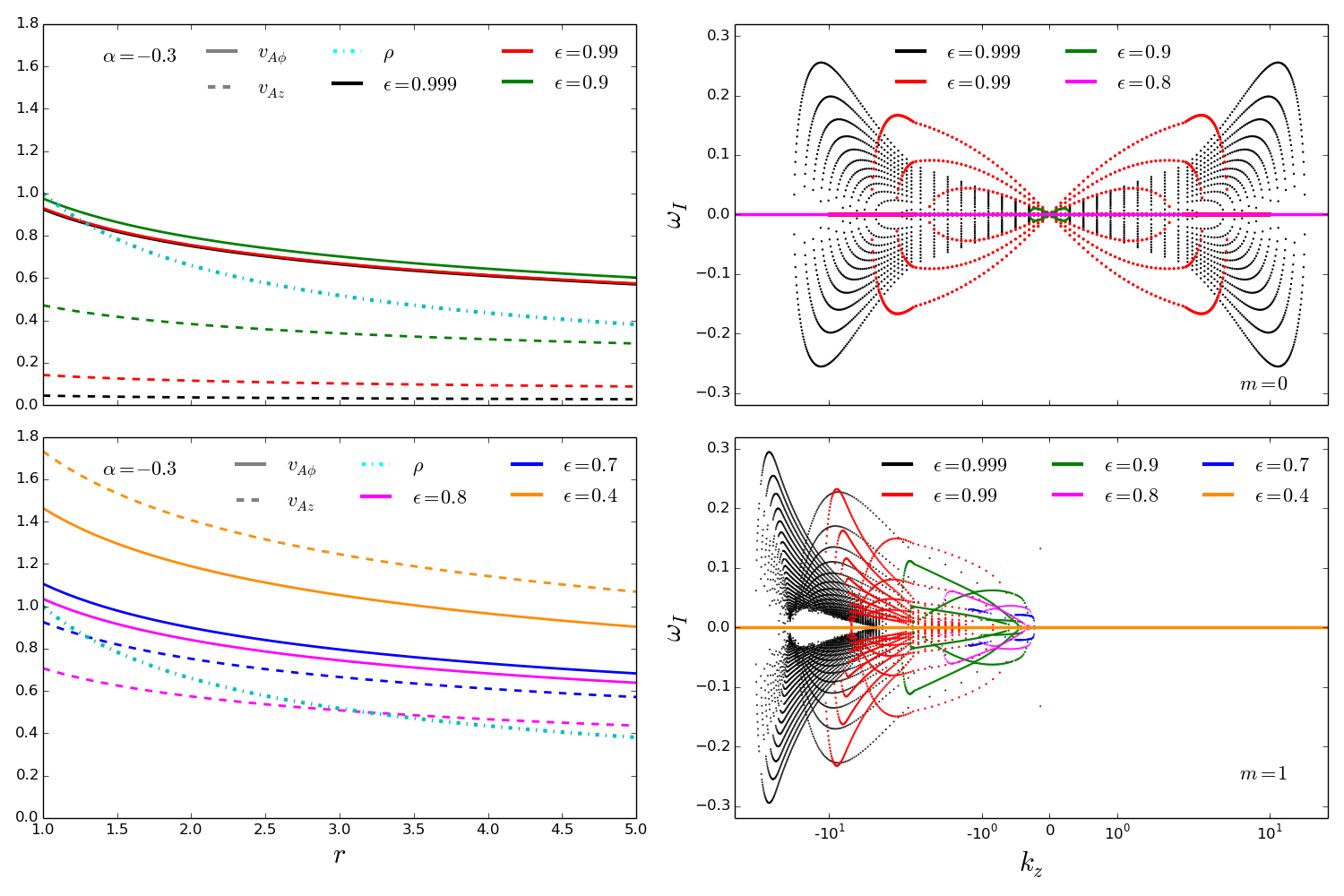
Figure 10: Global eigenvalue solutions for the case $v_{A\phi}{\rm-PL-}v_{Az}{\rm-Var}$ with $\alpha=-0.3$. Left panels: Background radial profiles of $v_{A\phi}$ (solid lines), $v_{Az}$ (dashed lines) and $\rho$ (cyan dot-dashed line) for different $\epsilon$ given by equation (38) (see colored legends; note that $\epsilon$ increases from top to bottom for the dashed curves). Right panels: Growth rate $\omega_{I}$ as a function of $k_{z}$ for the $m=0$ (top) and $m=1$ (bottom) cases, corresponding to the background profiles in the Left panels. Note that the maximum growth rate as well as the maximum unstable $|k_{z}|$ decreases as $\epsilon$ decreases.

5.2.1 Effect on $m=0$ and $m=1$ modes

The left panels of Figure 10 shows the profiles for the toroidal (solid) and vertical (dashed) fields as $\epsilon$ is varied, keeping $\alpha=-0.3$ fixed (top left: $\epsilon=0.999,0.99,0.9$; bottom left: $\epsilon=0.8,0.7,0.4$). The background density (and pressure) is independent of $\epsilon$ and is shown by the dot-dashed cyan line in the left panels (see equation 39). We see from the figure that for $\epsilon=0.999$, $v_{Az}$ is very subdominant compared to $v_{A\phi}$. Note that although $v_{A\phi}$ for $\epsilon=0.999$ and $\epsilon=0.99$ coincides (black and red solid lines in top left panel of Figure 10), $v_{Az}$ is different (black and red dashed lines in the same figure). As $\epsilon$ decreases, $v_{Az}$ approaches $v_{A\phi}$ quite steeply, and finally dominates over $v_{A\phi}$ when $\epsilon=0.4$. Note that since $v_{Az}$ follows the same power law as $v_{A\phi}$, the two profiles are identical when $v_{A\phi 0}=v_{Az0}$. This happens when $\epsilon=(1+2\alpha)/(1+\alpha)$, giving $\epsilon=0.57$ for $\alpha=-0.3$ and $\beta=0.667$. Thus, for $\epsilon<0.57$, the vertical field is stronger than the toroidal field.

The top right panel of Figure 10 shows the growth rates as a function of $k_{z}$ (from the global eigenvalue analysis) for the $m=0$ modes, when $\epsilon=0.999,0.99,0.9,0.8$. The bottom right panel shows the same for the $m=1$ modes, when $\epsilon=0.999,0.99,0.9,0.8,0.7,0.4$. We see that for both the axisymmetric and non-axisymmetric cases, as the vertical field gradient and strength become stronger compared to the thermal pressure gradient (which is independent of $\epsilon$), the growth rates decrease drastically. The $m=0$ modes appear to stabilize completely at a critical value, $\epsilon=\epsilon_{\rm cr}\sim 0.8$, contrary to the $m=1$ modes, which seem to persist under stronger vertical fields, and stabilize completely when $\epsilon_{\rm cr}\sim 0.4$. The $k_{z}>0$ modes for the $m=1$ case, however, stabilize for $\epsilon=0.999$. This is because the vertical field strength for this case is almost a factor of 10 higher at the inner boundary, i.e. $v_{Az0}=0.045$, compared to the fiducial $v_{A\phi}{\rm-PL-}v_{Az}{\rm-Cons}$ case shown in Figure 4 with $v_{Az0}=0.005$ (although the toroidal field profile remains similar for both the cases). This behavior is very similar to the stabilizing effect of a strong (constant) vertical field shown in Figure 7, and is likely due to current-driven effects.

Note that as the vertical field gradient, and hence strength, gets stronger, the instabilities shift to smaller $|k_{z}|$ and become increasingly Global in nature (and thus can no longer be captured in a local analysis). This makes determining a global stability criterion for this case more difficult, as the B98 stability criterion is not applicable in this limit (unlike in §5.1). Absolute stability is attained for a critical combination of the magnetic pressure gradients and the thermal pressure gradient in the jet, as indicated by $\epsilon_{\rm cr}$ (for a given $m$ and $\alpha$). In the case of $m\neq 0$ modes, this is similar to the statement of Suydam’s stability criterion, which however is not directly applicable in this case because of its local nature (see §3.4). Alternatively, it has been suggested by Bromberg & Tchekhovskoy (2016) that the internal kink instability (equivalent to the $m=1$ modes in this work) stabilizes when there is equipartition between the thermal and magnetic pressures. However, that seems to be neither a necessary nor a sufficient condition from our analysis. For instance, equipartition is attained when (in our units)

$$\rho=\frac{1}{2}(v_{A\phi}^{2}+v_{Az}^{2})$$ (43)

or, equivalently, $\beta=1$ in equation (41), which yields $\epsilon=0.71$ for $\alpha=-0.3$. However, from Figure 10 we see that the $m=0$ modes attain stability for $\epsilon>0.71$, when the thermal pressure dominates over the total magnetic pressure; while the $m=1$ modes attain stability for $\epsilon<0.71$, when the total magnetic pressure dominates over the thermal pressure. Although $\epsilon$ is just a parametrization, our results indicate that pressure balance alone may not guarantee stability, and one needs to consider the interplay between the magnetic and thermal pressure gradients as well (also, see §6 below).

Figure 11: Background radial profiles for the fiducial $v_{A\phi}{\rm-Gen-}v_{Az}{\rm-Cons}$ case, with $v_{A\phi}$ (solid line) given by equation (44), $\rho$ (dotted line) given by equation (46), $v_{A\phi 0}=0.447$, $a_{1}=0.1$ and $v_{Az}={\rm constant}=0.01$ (dashed line). The dot-dashed line shows a power-law profile for $v_{A\phi}=0.447r^{0.8}$.

5.3 Results for a generic toroidal field and constant vertical field: $v_{A\phi}{\rm-Gen-}v_{Az}{\rm-Cons}$

In this section, we consider a more generic profile for the background toroidal field such that

$$v_{A\phi}=v_{A\phi 0}\frac{(1+a_{1})r}{1+a_{1}r^{2}}~{},$$ (44)

where $a_{1}$ is a constant parameter governing the radial location of the peak of $v_{A\phi}$. The above equation mimics the magnetic field profiles obtained by Begelman & Li (1992) for their Crab Nebula models (see also Appl et al. 2000; O’Neill et al. 2012).

Table 6: Summary of runs for case $v_{A\phi}{\rm-Gen-}v_{Az}{\rm-Cons}$ presented in §5.3.

$m$	$a_{1}$	$v_{A\phi 0}$	$v_{A\phi 0}(1+a_{1})$	$v_{Az0}$	$N_{r}$	B.C.s imposed on $\rho(r)$	Other notes
$0,1,2$	$0.1$	$0.447$	$0.492$	$0.01$	$200$	$\rho(1)=1$; $\rho(r\rightarrow\infty)=0$	Fiducial model; $v_{A\phi 0}=\sqrt{2a_{1}}$
$1$	$0.2$	$0.447$	$0.537$	$0.01$	$200$	$\rho(1)=1$	$\rho\geq 0$ $\forall$ $r$
$1$	$0.3$	$0.447$	$0.581$	$0.01$	$200$	$\rho(1)=1$	$\rho\geq 0$ $\forall$ $r$
$1$	$0.4$	$0.447$	$0.626$	$0.01$	$200$	$\rho(1)=1$	$\rho\geq 0$ $\forall$ $r$
$1$	$0.5$	$0.447$	$0.671$	$0.01$	$200$	$\rho(1)=1$	$\rho\geq 0$ $\forall$ $r$

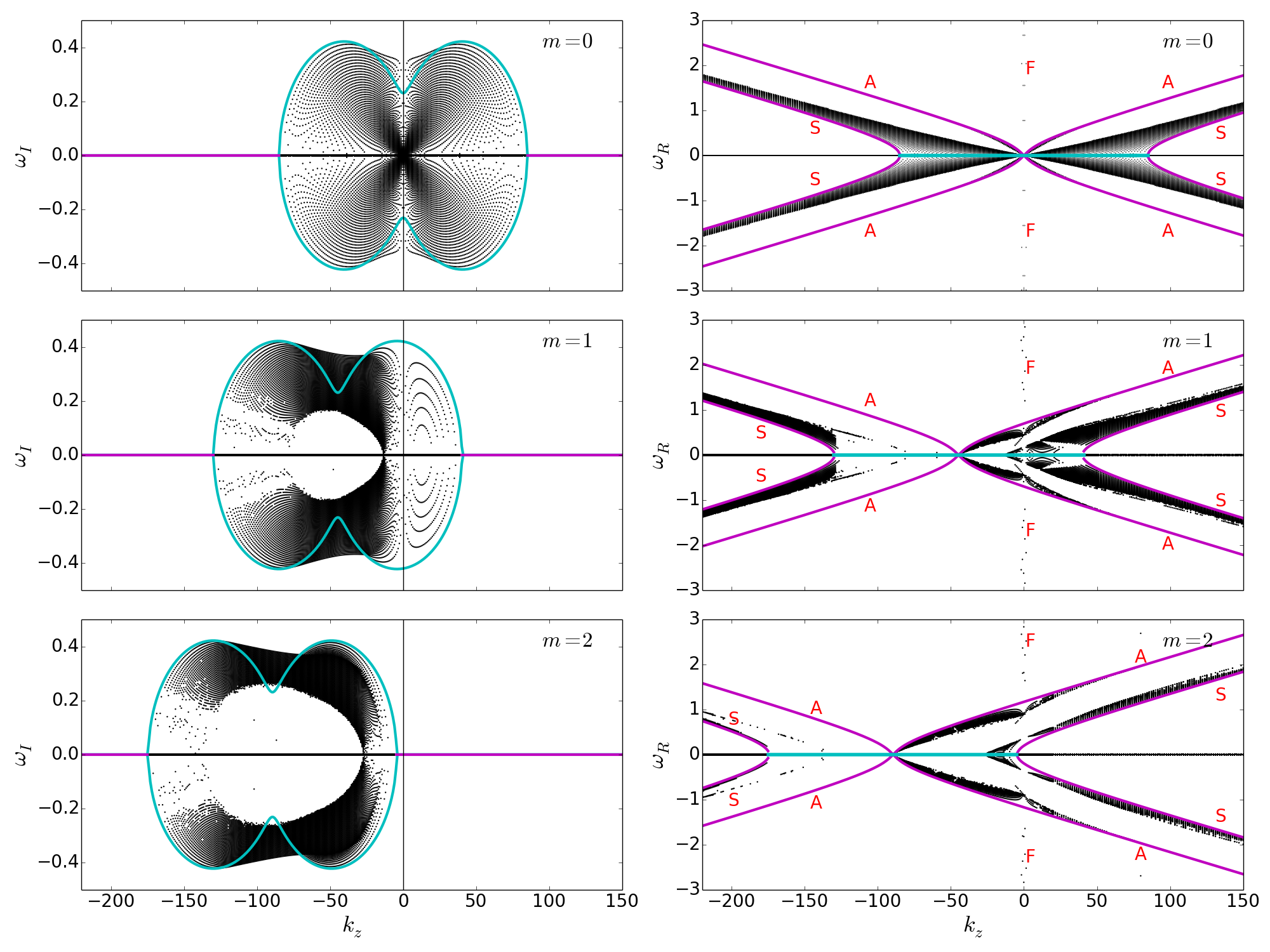
Figure 12: Global eigenvalue solutions for the fiducial $v_{A\phi}{\rm-Gen-}v_{Az}{\rm-Cons}$ case, with $v_{A\phi 0}=0.447$, $a_{1}=0.1$ and $v_{Az}=0.01$. The top, middle and bottom panels represent the $m=0,1$ and $2$ cases respectively. Left panels: Growth rate $\omega_{I}$ as a function of $k_{z}$. Right panels: The real part of the eigenvalue $\omega_{R}$ as a function of $k_{z}$. The cyan (unstable modes with $\omega_{I}>0$ and stable modes with $\omega_{I}<0$ in the left panels, and the corresponding $\omega_{R}$ in the right panels) and magenta (stable modes with $\omega_{I}=0$ in the left panels and the corresponding $\omega_{R}$ in the right panels) lines represent the solutions of the local dispersion relation, equation (11), for $v_{A\phi}=0.447r^{0.8}$, $v_{Az}=0.01$ and $l^{2}/k_{z}^{2}=0$. The global problem is solved on a radial grid $r\in[1,5]$ with resolution $N_{r}=200$. All symbols have the same meaning as in Figure 1.

Figure 13: Normalized radial eigenfunction $v_{1r}$ for the most unstable modes as a function of radius $r$, for the $m=1$ case shown in Figure 12 (see colored legends for $k_{z}$ values; note that $|k_{z}|$ increases from right to left in all panels). The red dashed vertical line, in the second panel from left, indicates the resonant radius $r_{\rm res}=3.82$ for $k_{z}=-20$ (red dashed curve), given by equation (20). Note that the radial axis in the last panel has been zoomed close to the inner boundary for clarity.

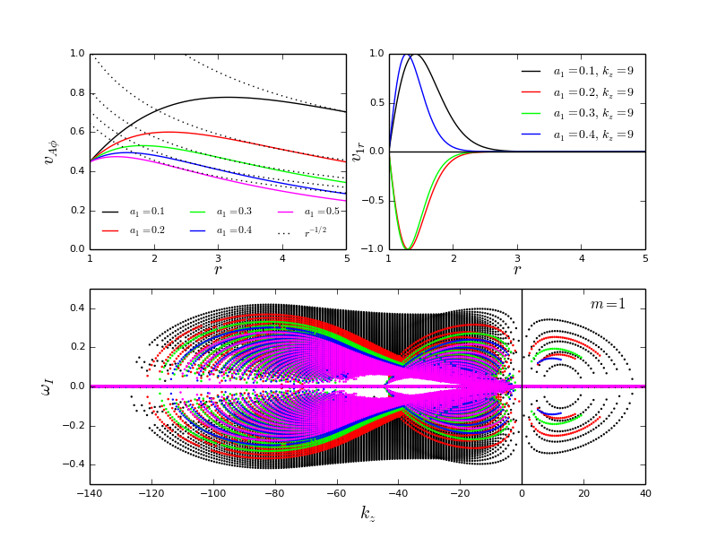
Figure 14: Global eigenvalue solutions for the $m=1$ case of $v_{A\phi}{\rm-Gen-}v_{Az}{\rm-Cons}$, when $v_{A\phi 0}=0.447$ and $v_{Az}=0.01$ are fixed, and $a_{1}$ is varied. Top left panel: Background radial profiles of $v_{A\phi}$ given by equation (44), with different $a_{1}$ (see colored solid curves; note that $a_{1}$ increases from top to bottom). The dotted lines represent the $r^{-1/2}$ profiles tangential to each $v_{A\phi}$. Bottom panel: Growth rate as a function $k_{z}$ for different $a_{1}$ (the color scheme is same as in top left panel; as $a_{1}$ increases, the maximum growth rate decreases). Top right panel: Normalized radial eigenfunction $v_{1r}$ as a function of $r$, corresponding to the most unstable mode at $k_{z}=9$ for different $a_{1}$ (note that $a_{1}$ increases from right to left).

We consider a constant vertical field $v_{Az}=v_{Az0}$, and obtain the density by integrating equation (7) subject to the boundary condition (31),

$$\rho(r)=1+\frac{v_{A\phi 0}^{2}(1+a_{1})^{2}}{2a_{1}}\biggl{(}\frac{1}{(1+a_{1}r^{2})^{2}}-\frac{1}{(1+a_{1})^{2}}\biggr{)}~{}.$$ (45)

For our fiducial model, we also impose the boundary condition (34) to obtain

$$\rho(r)=\frac{(1+a_{1})^{2}}{(1+a_{1}r^{2})^{2}}~{}~{}{\rm and}~{}~{}v_{A\phi 0}=\sqrt{2a_{1}}~{}.$$ (46)

The plasma-beta for the fiducial model, on assuming $v_{Az0}\ll v_{A\phi}$, then becomes

$$\beta\approx\frac{1}{a_{1}r^{2}}~{}.$$ (47)

The pitch for this magnetic configuration follows from equation (6):

$${\cal P}=\frac{v_{Az0}(1+a_{1}r^{2})}{v_{A\phi 0}(1+a_{1})}~{},$$ (48)

which increases with radius. Figure 11 shows the different background profiles as a function of $r$ for our fiducial case having $a_{1}=0.1$, $v_{A\phi 0}=0.447$ and $v_{Az0}=0.01\ll v_{A\phi 0}$. We use $r\in[1,5]$ for all the cases studied in this section, which are listed in Table 6. Figure 12 shows $\omega_{I}$ (left panels) and $\omega_{R}$ (right panels) as a function of $k_{z}$ for the $m=0$ (top), $m=1$ (middle) and $m=2$ (bottom) modes described by the fiducial model shown in Figure 11. The global eigenvalue solutions are in black, while the cyan ($\omega_{I}\neq 0$) and magenta ($\omega_{I}=0$) lines indicate local solutions derived using the B98 dispersion relation with $l^{2}/k_{z}^{2}=0$ (equation 11) for a power-law toroidal field $v_{A\phi}=0.447r^{0.8}$. Note that there is no fixed $\alpha$ corresponding to the generic profile, however, a slope of $\alpha=0.8$ is tangent to the generic profile at the inner radius (see Figure 11). This gives us the opportunity to directly compare the solutions of the generic and power-law toroidal fields. Note that all colors and symbols have the same meaning as in Figure 1. The main findings of this section, discussed below, are summarized by Figures 12, 13 and 14:

1. The growth rates of the $m=0$ modes are symmetric about the $k_{z}$-axis, as expected. The global solution matches well with the local solution (representing the most unstable modes) for $|k_{z}|\gtrsim 30$. The local power law solution predicts a maximum growth rate $\omega_{g}|_{\rm max}\approx 0.42$ (see equation 17), the corresponding vertical wavenumbers $k_{z}|_{\rm max}\approx\pm 40$ (see equation 19) and the range of instability $-85\lesssim k_{z}|_{\rm unst}\lesssim 85$ (see relation 15). All the corresponding global quantities are in very good agreement but with slightly lower values. However, the growth rates are somewhat higher than the local prediction for $|k_{z}|<30$. Note that unlike the $m=0$ case for $\alpha=-0.3$ shown in Figure 1, the most unstable modes do not have $\omega_{I}\rightarrow 0$ as $k_{z}\rightarrow 0$. This can be explained by the fact that the present solution is roughly approximated by a $\alpha>0$ power-law toroidal field, which tends to give higher growth rates because $v_{A\phi}$ is increasing with radius. Thus, the solutions behave differently from our fiducial $\alpha<0$ case (see §5.1.1).

2. The envelope of the global solutions for both the $m=1$ and $m=2$ cases, i.e. the most unstable modes, seem to match reasonably well with the local prediction, with some differences. The local solutions for both $m=1$ and $2$ have a double peaked structure. This is again due to the occurrence of local magnetic resonance at $r=1$ for $m=1$ with $k_{z}|_{\rm res}=-v_{A\phi 0}/v_{Az0}\approx-45$; and for $m=2$ with $k_{z}|_{\rm res}=-2v_{A\phi 0}/v_{Az0}\approx-89$. However, $\omega_{I}\neq 0$ at $k_{z}|_{\rm res}$, unlike the behavior of the local resonance discussed in §5.1.2. The two peaks in the global solution are barely distinguishable due to slow-mode-slow-mode interaction, leading to a band of higher growth rate about $k_{z}\approx-45$ for $m=1$ and about $k_{z}\approx-89$ for $m=2$. For $m=1$, the local solution slightly overestimates the growth rates for the $k_{z}>0$ modes, as well as that of the first peak. For $m=2$, the $k_{z}>0$ modes are completely stabilized, however the $k_{z}<0$ modes start slightly further away from the axis than the local prediction. In both cases, the local solution predicts the total range of instability extremely well.

3. From the right panels of Figure 12, we find that the most unstable modes are destabilized slow modes that are purely growing, for all $m=0,1$ and $2$ cases. In fact, the local predictions match quite well with the global solutions across all $k_{z}$ and $m$, with no new branches of slow-Alfvén interaction appearing in the $\omega_{R}-k_{z}$ plane, unlike those observed in §5.1.

4. In Figure 13, we illustrate the normalized, $v_{1r}$ eigenfunctions corresponding to the most unstable $m=1$ modes. The $k_{z}>0$ modes shown in the first panel (from left) are Global II stabilities, which tend to get more localized to the inner boundary as $k_{z}$ increases. The unstable modes in the range $-20\leq k_{z}\leq-5$ shown in the second panel also represent Global II instabilities, however with a larger $\Delta r$ than the first panel. The third panel showing $-70\leq k_{z}\leq-30$ represent Global III instabilities, i.e. the interacting slow modes. Finally, the last panel showing $-125<k_{z}<-85$ represents Local instabilities.

   Note that the $m=1$ modes satisfying the magnetic resonance condition for the present field profile are given by $k_{z}=-(v_{A\phi 0}/v_{Az0})(1+a_{1})/(1+a_{1}r^{2})$. Thus, for $r\in[1,5]$, the modes in $-45\lesssim k_{z}\lesssim-14$ are supposed to be resonant. Again, the most unstable modes in $-45\lesssim k_{z}\lesssim-30$ are interacting and non-resonant (third panel), while the eigenfunctions of the modes in $-20\lesssim k_{z}\lesssim-14$ peak far away from the resonant radius (second panel). For example, the eigenfunction for $k_{z}=-20$ peaks at $r\sim 1.35$, which is inside the resonant surface for this mode at $r_{\rm res}=\sqrt{(1/a_{1})(-1-v_{A\phi 0}(1+a_{1})/(k_{z}v_{Az0}))}\sim 3.82$ (vertical red dashed line in second panel of Figure 13). This is similar to the conclusion drawn regarding the unstable modes discussed in §5.1.2.

   As to the eigenfunctions of the most unstable $m=0$ modes, they represent Global I instabilities for $|k_{z}|<15$, Global II instabilities for $15<|k_{z}|<30$ and Local instabilities for $|k_{z}|>30$ — which corroborates the deviation of the global solution from the local prediction at small $|k_{z}|$. The eigenfunctions of the most unstable $m=2$ modes represent Global II instabilities for $-40<k_{z}<-10$, Local instabilities for $-70<k_{z}<-40$, Global III instabilities for $-115<k_{z}<-70$ (interacting modes), and again Local instabilities for $-170<k_{z}<-115$.

5. Finally, in Figure 14, we compare the global solutions for the $m=1$ modes corresponding to multiple generic profiles having different $a_{1}$. The toroidal magnetic fields (colored solid lines) are shown as a function of radius in the top left panel. They are constructed such that they all have the same $v_{A\phi 0}=0.447$ and $v_{Az}=constant=0.01$ as the fiducial model (see Table 6 for details). We note that as $a_{1}$ increases, the maximum magnetic field strength decreases as well as shifts towards the inner boundary. The dotted lines are $\propto r^{-0.5}$, which become tangential to the different magnetic field curves at different radii. The aim here is to establish a correlation with the solutions of the power-law profiles discussed in §5.1.

   The bottom panel shows the growth rate as a function of $k_{z}$ corresponding to the cases in the top left panel (global eigenvalue solutions only). We observe that as $a_{1}$ increases, the growth rates of the unstable modes decrease and the range of instability shrinks. Furthermore, the two growth rate peaks (for $k_{z}<0$) become more distinguishable and the modes start resembling the left panel of Figure 4. Interestingly, the $k_{z}>0$ modes stabilize for $a_{1}>0.4$, which we now try to explain using the top two panels (note that some of the incomplete $k_{z}>0$ curves are due to inadequate resolution).

   In §5.1.2 and Figure 6, we saw that the $k_{z}>0$ modes are completely stabilized when $\alpha=-0.5$ as per B98 prediction. Keeping that in mind, in the top left panel of Figure 14 we observe that the radius at which the $r^{-0.5}$ curve is tangential to the respective field profiles shifts radially inwards as $a_{1}$ increases. Now, the most unstable $k_{z}>0$ mode for each $a_{1}$ roughly corresponds to $k_{z}=9$ (see bottom panel). The top right panel shows the $v_{1r}$ eigenfunctions for $k_{z}=9$ when $a_{1}=0.1,0.2,0.3$ and $0.4$. All four eigenfunctions represent Global II instabilities, which implies that they are influenced by the background toroidal field profile. More interestingly, the eigenfunctions also shift radially inwards as $a_{1}$ increases. Thus, we can conclude that if the toroidal field transitions to a $r^{-0.5}$ at sufficiently small radii to influence the eigenfunctions of the $k_{z}>0$ unstable modes, they get stabilized. For the present scenario, this happens when $a_{1}=0.5$. Similarly, we can conclude that there will be complete stabilization (i.e. of all $k_{z}$ modes) with a further increase in $a_{1}$, as the background toroidal field transitions to a $r^{-1}$ profile. Thus, we recover the B98 stability criterion even for a more complex magnetic background, precisely due to the local nature of the fastest growing internal (pressure-driven) instabilities (provided $v_{Az}\ll v_{A\phi}$).

6 Discussion

In this section, we discuss some of our results in the context of recent numerical simulations.

Bromberg & Tchekhovskoy (2016) carried out global, 3D relativistic MHD simulations of relativistic, Poynting-flux-dominated jets. They simulated 2 kinds of jets — (1) headless jets that propagate in a vacuum funnel and experience no direct influence from the ambient medium; and (2) headed jets that propagate through an ambient medium. They found that the ambient medium is responsible for collimating the headed jets, and that this compression effect triggers the internal kink instability (and, also, the external kink instability that we do not discuss here). Since these instabilities lead to the dissipation of magnetic energy, the simulations showed a build-up of background thermal pressure, which can no longer be ignored under the force-free approximation. One of the main findings of Bromberg & Tchekhovskoy (2016) was that the internal kink instabilities saturated once equipartition was reached between the thermal and magnetic energies, about which we commented briefly in §5.2 above. In Figure 15, we reconstruct a situation similar (but not identical) to that in Fig. 14 of Bromberg & Tchekhovskoy (2016), to analyze the conditions under which the internal kink stabilizes.

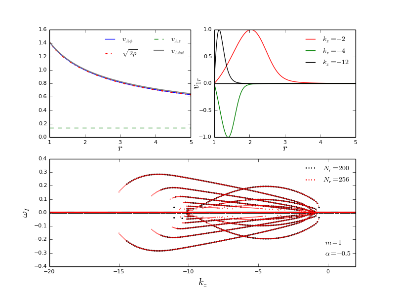
Figure 15: Testing the role of equipartition between thermal and magnetic pressures on the stability of $m=1$ modes. Top left panel: Background radial profiles of a toroidal Alfvén velocity $v_{A\phi}=1.41r^{-0.5}$ (blue solid line), constant vertical Alfvén velocity $v_{Az}=0.14$ (green dashed line), total Alfvén velocity $v_{Atot}=\sqrt{v_{A\phi}^{2}+v_{Az}^{2}}$ (solid gray line) and $\sqrt{2\rho}$, which is a quantity proportional to the thermal pressure (red dot-dashed line), so defined to compare with the Alfvén velocities. Bottom panel: Growth rate as a function of $k_{z}$ from the global eigenvalue analysis of the case shown in the top left panel for $m=1$, and radial grid resolutions $N_{r}=200$ (black) and $N_{r}=256$ (red). Top right panel: Normalized radial eigenfunction $v_{1r}$ as a function of $r$, corresponding to the most unstable modes at $k_{z}=-2,-4,-12$ (see colored legends for $k_{z}$ values; note that $|k_{z}|$ increases from right to left).

In their Fig. 14, Bromberg & Tchekhovskoy (2016) showed the azimuthally averaged, magnetic field and thermal pressure profiles inside their 3D simulated jet, at a height where there was no more dissipation due to the internal kink instability. The top left panel of our Figure 15 shows a power-law profile for the toroidal field (solid blue line) such that $\alpha=-0.5$ and $v_{A\phi 0}=1.41$ (see equation 35), in order to match the scaling found by Bromberg & Tchekhovskoy (2016). The ratio of the vertical to toroidal field strength is roughly similar to that in Fig. 14 of Bromberg & Tchekhovskoy (2016), such that we choose $v_{Az}=0.14$ (dashed green line). Note that our vertical field is constant, unlike Bromberg & Tchekhovskoy (2016) (we shall comment on this later). In order to compare the thermal pressure with the magnetic fields, we plot the equivalent quantity given by equation (43), i.e. $\sqrt{2\rho}$ (red dot-dashed line). We see that for this case, the thermal pressure is in exact equipartition with the toroidal field, and very nearly in equipartition with the total magnetic field, $v_{Atot}=\sqrt{v_{A\phi}^{2}+v_{Az}^{2}}$ (gray solid line). Since our computational domain is located away from the jet boundaries and core, this plot can be compared with the toroidally dominated regime in Fig. 14 of Bromberg & Tchekhovskoy (2016), i.e. the outer jet region from $\sim 20-60R_{L}$, where $R_{L}$ is the light cylinder radius in their work (we have kept the same color and line-style scheme in the top left panel of our figure as Fig. 14 of Bromberg & Tchekhovskoy (2016) for easier comparison). The main point of this exercise is to demonstrate that despite equipartition, as well as the $r^{-0.5}$ scaling for $v_{A\phi}$, we find unstable $m=1$ modes in our analysis (with a non-negligible maximum growth rate $\sim 0.3$), unlike Bromberg & Tchekhovskoy (2016). Note that the bottom panel of Figure 15 presents solutions for two resolutions $N_{r}=200$ and $N_{r}=256$. This is to show that the apparent gaps in the solutions towards higher $|k_{z}|$ are not real, and they close as the resolution increases. The eigenfunctions of the most unstable modes at $k_{z}=-2,-4,-12$ are plotted in the top right panel. We shall now discuss a few possible explanations for this apparent discrepancy.

First, we check if the the above eigenfunctions can be resolved in the set-up employed by Bromberg & Tchekhovskoy (2016), who use a logarithmic radial grid with a uniform (dimensionless) spacing $r_{grid}=(r_{br}/r_{in})^{1/N}-1$, where $N$ is their radial grid resolution, and $r_{in}=0.8R_{L}$ and $r_{br}=800R_{L}$ are the inner and outer radial boundaries (see their Table 1). They use two resolutions, namely, $N=128$ and $N=256$, which correspond to $r_{grid}\sim 0.06$ and $0.03$ respectively. The dimensionless quantity describing our eigenfunctions, equivalent to $r_{grid}$, is therefore $\Delta r/r_{1}$ (see top left panel of Figure 2). We see that as $|k_{z}|$ increases, the eigenfunctions in the top right panel of Figure 15 become more localized towards the inner boundary having $\Delta r/r_{1}\sim 0.7,0.4,0.24$ for $k_{z}=-2,-4,-12$ respectively. We next define a quality factor ${\cal Q}=(\Delta r/r_{1})/r_{grid}$, which determines how well resolved an eigenfunction is. Although Fig. 14 of Bromberg & Tchekhovskoy (2016) is for the $N=128$ case, we compare our eigenfunctions with their higher resolution case $N=256$. We find that for $r_{grid}\sim 0.03$ the eigenfunctions appear to be well-resolved, having ${\cal Q}=23,13,8$ for $k_{z}=-2,-4,-12$ respectively. Thus, in principle, the unstable modes we find in our Figure 15 should have led to the internal kink instability in the 3D jets simulated by Bromberg & Tchekhovskoy (2016).

Next, we take a closer look at Fig. 14 of Bromberg & Tchekhovskoy (2016) and point out its differences with our Figure 15. We observe from Fig. 14 of Bromberg & Tchekhovskoy (2016) that although the very inner core of the jet (which we exclude from our computation) is indeed in equipartition, the outer jet region, $\sim 20-60R_{L}$, is not. In fact, the thermal pressure dominates over the magnetic pressure in the outer region. Interestingly, the thermal pressure profile is nearly flat in this region, which in turn implies a very weak thermal gradient. This is probably a consequence of the rapid thermal pressure build up due to magnetic energy dissipation. Moreover, the vertical field has a non-negligible gradient, and its strength, although less than the toroidal field, cannot be considered as sub-dominant (hence the B98 stability criterion cannot be applied in this case). Thus, we believe that the main cause for stability seen in Bromberg & Tchekhovskoy (2016) is the negligible thermal pressure gradient in the jet region above the dissipation zone, which is easily stabilized by the combined vertical and toroidal field gradients present therein (as discussed in §5.2).

Our stability analysis is also consistent with the “core-envelope” jet model of Komissarov (1999), which was used to carry out periodic box, 3D simulations by Porth & Komissarov (2015). This model consists of a Z-pinched inner jet core, where the toroidal field balances the plasma pressure, and a force-free, purely toroidal outer envelope such that $B_{\phi}\propto 1/r$. Note that the main objective of Porth & Komissarov (2015) was to investigate the stability of their jet to external, large-scale instabilities by exploring different pressure distributions for the ambient medium. They found that for a critical ambient pressure ($P_{\rm amb}\propto z^{-2}$) the overall jet becomes stable to the external instabilities, the outer envelope is featureless, and the internal instabilities are confined to a narrow jet core. We point out that irrespective of the nature of the ambient medium and the jet core (both of which are excluded from our analysis), the outer envelope would be stable to all internal instabilities according to the B98 stability criterion (see §3.2), which has been extensively verified in this work (see §5.1). Thus, if an unstable jet core additionally develops, the magnetic energy would be dissipated to heat by the internal instabilities therein. This would lead to a bright core or spine, which would in turn be surrounded by a stable and darker envelope or sheath, giving rise to the so-called “spine-sheath” structure, commonly invoked to explain observations of jets in AGN (e.g. Mimica et al., 2015) and blazars (e.g. Sikora et al., 2016).

In an earlier study, Mizuno et al. (2012) also carried out 3D relativistic, periodic box, MHD simulations of rotating jets, having a poloidal field dominated core and $B_{\phi}\rightarrow 1/r$ in the envelope. They considered a low gas density and pressure background decreasing with radius such that their jets were still force-free. They found that the jets were helically distorted due to the development of the internal kink instability, whose growth rate depended strongly on the gradient of the poloidal field. Their findings were in accord with the linear stability analyses mentioned in our Introduction (Istomin & Pariev, 1996; Lyubarskii, 1999), which in turn emphasizes the relevance of linear studies. Mizuno et al. (2012) further found that multiple unstable wavelengths were excited during the non-linear evolution, which coupled to give rise to an external kink instability that disrupted the entire jet. We consider Fig. 8 of Mizuno et al. (2012), which shows the time evolution of 2D density slices in the $xz$-plane of the jet ($z$ being the jet-axis), for different angular velocities. If we interpret the loop-like, high density structures in this figure (denoted by orange and red) as locations where the internal kink instability is triggered, we observe that they are localized in the interior of the jet (for all the panels). However, there is no instability seen towards the edge of the jet where $B_{\phi}\propto 1/r$, which is again compatible with the B98 stability criterion.

Finally, we discuss the 3D resistive MHD simulations by Striani et al. (2016) to highlight the significance of thermal pressure gradients. These were performed to study reconnection in magnetically confined cylindrical plasma columns. Striani et al. (2016) modeled both a force-free equilibrium, as well as one with a thermal pressure gradient. For the latter case, they found small-scale, finger-like structures in the current density triggered by the pressure-driven, internal kink instability (see their Fig. 7). These features were shown to cause efficient magnetic dissipation via reconnection of multiple fragmented current sheets, which in turn reinforces the premise of our work. For the force-free case, Striani et al. (2016) observed a bending of the plasma column due to the current-driven kink instability as well as the formation of plume-like structures (see their Fig. 9). More interestingly, they found that the currents through several plumes were perpendicular to the magnetic field, indicative of a secondary pressure-driven instability (as the Lorentz force is required to be balanced by a non-zero thermal pressure gradient in these regions; see their Fig. 10), which led to formation of mixed modes. Fragmentation of current sheets and an enhanced magnetic dissipation rate were also noted in this case. This finding leads to the important inference that initially Poynting flux dominated jets can also develop thermal pressure gradients, which in turn are essential to facilitate magnetic reconnection and dissipation.

7 Summary and conclusions

Below we summarize the main findings of our analysis:

• We have carried out a global eigenvalue analysis of the linearized, ideal MHD equations, in order to study the stability of cylindrical jets to both axisymmetric and non-axisymmetric perturbations. Our calculations have been performed in the jet fluid frame, and we have ignored velocity shear (both at the surface as well as in the interior), rotation and relativistic effects for simplicity. We have focused on characterizing the small-scale, internal instabilities that are confined to the interiors of jets, away from the effects of both the jet core and boundaries. We have further analyzed the importance of a thermal pressure gradient for triggering instabilities in a region of the jet dominated by a toroidal magnetic field (with a sub-dominant vertical field), as is likely to occur at some distance from the jet source. This gives rise to predominantly pressure-driven instabilities, which are often overlooked in the literature compared to their purely current-driven counterparts arising in force-free jets. Since the exact transverse structure of magnetic fields inside jets is not known, we have adopted three different background configurations for our stability analysis, yielding the results summarized below.

  Before we proceed with the summary, note that we have further classified the internal instabilities as Local and Global, based on the properties of their radial eigenfunctions (see Table 4 for details). The Local instabilities have narrow eigenfunctions and peak very close to the inner radial boundary. Hence, these agree very well with local (i.e. radially localized) analytic calculations. The Global instabilities fall into several different types, any of which can be captured accurately only in a global (radially extended) framework as they are influenced by the background radial gradients and curvature (again, not to be confused with large-scale external instabilities). Note that all the instabilities found in this work are purely growing slow magnetosonic modes.

• First, we have considered a power-law profile for the toroidal magnetic field, such that $v_{A\phi}\propto r^{\alpha}$, and a constant vertical magnetic field $v_{Az}$ (§5.1; case $v_{A\phi}{\rm-PL-}v_{Az}{\rm-Cons}$). We do a parameter scan for different values of $\alpha$, and find internal instabilities for a range of vertical wavenumbers $k_{z}$ (both $k_{z}>0$ and $k_{z}<0$; the sign indicates the direction of the helical twist with respect to the magnetic field if $m>0$), for $m=0,1,2$ (see Figures 1, 4 and 8). The maximum growth rate (which is nearly independent of $m$, as is characteristic of pressure-driven instabilities) for a given $\alpha$, matches very well with the predictions of B98, who performed a local, linear stability analysis of a similar jet model. Interestingly, we find that in a region where $v_{Az}\ll v_{A\phi}$, all ($m,k_{z}$) modes are stabilized for $\alpha\leq-1$ (see e.g. Figures 3 and 6). This global stability criterion is in excellent agreement with the local criterion of B98. This criterion is better understood by looking at the radial equilibrium equation (9), which shows that the thermal pressure gradient (or equivalently, density gradient in our case) has a negative sign in general (for $\alpha>-1$), and is oppositely directed to the restoring magnetic tension force. However, when $\alpha=-1$, the thermal pressure gradient vanishes, the toroidal magnetic pressure gradient is balanced by its own tension force and the system becomes stable irrespective of $m$ and $k_{z}$. Note that for $m=1$, the $k_{z}>0$ modes get stabilized at a shallower toroidal field profile, i.e. $\alpha\lesssim-0.5$, which is also in direct corroboration with B98. In a region where $v_{Az}$ is comparable to $v_{A\phi}$, however, the modes get stabilized even for $\alpha>-1$ (Figure 7).

  The $m=0$ unstable modes can be classified as Local instabilities across almost their entire $k_{z}$-range (Figure 2). The global solutions for the $m\neq 0$ cases, however, exhibit a mixture of Local and Global instabilities. The Global instabilities tend to occur at smaller $|k_{z}|$, and also include those arising due to the interaction between distinct slow modes occupying the same range of $k_{z}$ (Figures 5 and 9). Nevertheless, the fastest growing modes for all $m$ are Local instabilities, which occur predominantly at large negative values of $k_{z}$. This is the reason for the excellent agreement between B98’s local analysis and our global solutions. The important consequence of this finding is as follows: in a toroidally dominated region of a jet with a negative thermal pressure gradient strong enough to trigger instability (and very weak vertical field), internal instabilities can occupy any local patch of the jet, irrespective of the exact configuration of the magnetic field in the jet interior. According to B98, the growth timescales of these instabilities are inversely proportional to the toroidal field strength; thus, they grow fast enough for a substantial region of the jet to become internally unstable. This in turn can serve as a likely site for dissipation of magnetic energy to heat (and non-thermally accelerated particles) via current sheet formation. The Global instabilities, which are subject to the details of the radial profiles, would further enhance this effect. Although internal instabilities can develop close to the base of Poynting-flux-dominated jets (e.g. Bromberg & Tchekhovskoy, 2016), we propose that a thermal pressure gradient is crucial to sustain them farther from the source, where much of the particle acceleration leading to radiation takes place.

• Next, we have considered the same toroidal field profile as above but with a radially varying vertical magnetic field (§5.2; case $v_{A\phi}{\rm-PL-}v_{Az}{\rm-Var}$). In order to self-consistently determine the equilibrium, we have assumed the vertical magnetic pressure to be proportional to the thermal pressure, characterized by the parameter $\epsilon$ (see equation 38) — the smaller the value of $\epsilon$, the stronger the vertical magnetic field. As the vertical field gradient increases (for a given $\alpha$), there is a consequent increase in the vertical field strength relative to the toroidal magnetic field, although the thermal pressure gradient remains unchanged (as it is independent of $\epsilon$ in this formalism). A decrease in $\epsilon$ induces stabilization of both the $m=0$ and $m=1$ modes for a given $\alpha$ (Figure 10). Complete stabilization for the $m=0$ and $m=1$ modes are, however, attained at different values of $\epsilon$, indicating that the pinch and kink modes react differently to the background gradients. Moreover, our results indicate that stability in such a situation is not determined solely by whether equipartition is achieved between the thermal and magnetic pressures (see the last point below).

• Finally, we have considered a more complex toroidal field profile (see equation 44) with a constant (weak) vertical magnetic field (§5.3; case $v_{A\phi}{\rm-Gen-}v_{Az}{\rm-Cons}$). Interestingly, we find that for all the $m=0,1$ and $2$ cases, the growth rate and the $k_{z}$-range of instability of the most unstable global solutions show excellent agreement with the corresponding local solutions obtained for a power-law toroidal field with $\alpha=0.8$ and the same $v_{A\phi 0}$ (see Figures 11 and 12). We have also established a direct correlation between the stability criterion for the complex toroidal field configuration and the simple power-law configuration. We find that as the background toroidal field becomes proportional to $r^{-1/2}$, i.e. $\alpha=-0.5$, the $k_{z}>0$ modes get completely stabilized for $m=1$, as in the power-law case (see Figure 14). A similar line of reasoning allows us to conclude that the B98 stability criterion for all $k_{z}$-modes (i.e. $\alpha\leq-1$) would also be valid be in this case. The $m=0$ modes again represent mostly Local instabilities, whereas the $m\neq 0$ modes exhibit both Global and Local instabilities, occupying different $k_{z}$. As $k_{z}$ assumes increasingly negative values, however, the instabilities become more and more localized close to the inner radial boundary for the non-axisymmetric case (see Figure 13). This further validates our claim that highly localized internal instabilities are triggered as long as the B98 instability criterion is satisfied locally inside the jet, irrespective of the background magnetic field profile. We have also established that magnetic resonance does not play any role in triggering the $m\neq 0$ instabilities (irrespective of the toroidal field profiles), as their eigenfunctions peak far away from the corresponding resonant radii (see §3.3, and second panels of Figures 5, 9 and 13).

• We have also compared our results with those of recent 3D numerical simulations by Mizuno et al. (2012); Porth & Komissarov (2015); Bromberg & Tchekhovskoy (2016) and Striani et al. (2016). We conclude that thermal pressure gradients are indeed key to incite internal instabilities, which are fundamental for causing magnetic energy dissipation via reconnection of current sheets. With regards to the question of what causes internal instabilities to saturate, our results indicate two possible answers depending upon the region of the jet in question: (1) in a toroidally dominated region with a very weak vertical field, complete stability for all $m$-modes is attained when the toroidal field behaves as $v_{A\phi}\propto 1/r$, as proposed by B98. This supports the “spine-sheath” model of jets, with a Z-pinched jet core and an envelope stable to internal instabilities, observed in several AGN jets; (2) in a region with appreciable toroidal field but a non-negligible vertical field strength and radial gradient, stability ultimately ensues from the complex interplay between the destabilizing thermal pressure gradient and the stabilizing magnetic pressure gradients, or equivalently, magnetic shear. Contrary to the claim by Bromberg & Tchekhovskoy (2016), we conclude that equipartition alone may not guarantee stability (see Figure 15). Both of these situations are possible in a real jet (at different distances from the source), depending upon how fast the vertical field falls off relative to the toroidal field due to either the lateral expansion of the jet (Begelman et al., 1984) or the divergence of outer flux surfaces (Begelman & Li, 1994).

Appendix A Linearized MHD equations

In order to carry out a linear stability analysis, we perturb the MHD equations (1), (2), (4) and (5), and retain only the terms of linear order such that

$$\rho=\rho_{0}+\rho_{1}~{},$$ (49)

$$P=P_{0}+P_{1}~{},$$ (50)

$${\bf v}={\bf v_{1}}~{},$$ (51)

$${\bf B}={\bf B_{0}}+{\bf B_{1}}~{},$$ (52)

$${\bf A}={\bf A_{0}}+{\bf A_{1}}~{}.$$ (53)

We can now write the complete set of the linearized MHD equations for a generic case involving non-axisymmetric perturbations, background radial gradients, compressibility and radial curvature:

$$\partial_{t}\rho_{1}+\rho_{0}\biggl{[}\frac{1}{r}\partial_{r}(rv_{1r})+\frac{1}{r}\partial_{\phi}v_{1\phi}+\partial_{z}v_{1z}\biggr{]}+v_{1r}\partial_{r}\rho_{0}=0~{},$$ (54)

$$\rho_{0}\partial_{t}v_{1r}+\partial_{r}\rho_{1}+\frac{1}{4\pi}\biggl{[}B_{0\phi}\partial_{r}B_{1\phi} +B_{1\phi}\partial_{r}B_{0\phi}-\frac{B_{0\phi}}{r}\partial_{\phi}B_{1r}-B_{0z}\partial_{z}B_{1r}+B_{0z}\partial_{r}B_{1z}+\frac{2B_{0\phi}B_{1\phi}}{r}+B_{1z}\partial_{r}B_{0z}\biggr{]}=0~{},$$ (55)

$$\rho_{0}\partial_{t}v_{1\phi}+\frac{1}{r}\partial_{\phi}\rho_{1}-\frac{1}{4\pi}\biggl{[}B_{1r}\partial_{r}B_{0\phi}+B_{0z}\partial_{z}B_{1\phi}-\frac{B_{0z}}{r}\partial_{\phi}B_{1z}+\frac{B_{0\phi}B_{1r}}{r}\biggr{]}=0~{},$$ (56)

$$\rho_{0}\partial_{t}v_{1z}+\partial_{z}\rho_{1}+\frac{1}{4\pi}\biggl{[}B_{0\phi}\partial_{z}B_{1\phi}-\frac{B_{0\phi}}{r}\partial_{\phi}B_{1z}-B_{1r}\partial_{r}B_{0z}\biggr{]}=0~{},$$ (57)

$$B_{1\phi}-\partial_{z}A_{1r}+\partial_{r}A_{1z}=0~{},$$ (58)

$$B_{1z}+\partial_{r}A_{1\phi}-\frac{1}{r}\partial_{r}(rA_{1r})=0~{},$$ (59)

$$\partial_{t}A_{1r}-B_{0z}v_{1\phi}+B_{0\phi}v_{1z}=0~{},$$ (60)

$$\partial_{t}A_{1\phi}+B_{0z}v_{1r}=0~{},$$ (61)

$$\partial_{t}A_{1z}-B_{0\phi}v_{1r}=0~{},$$ (62)

where the relation $P_{1}=c_{s}^{2}\rho_{1}$ has been used to eliminate $P_{1}$. Note that $B_{1r}$ is not an independent quantity as it can be defined as $B_{1r}=\partial_{\phi}A_{1z}/r-\partial_{z}A_{1\phi}$. This set of 9 equations for the 9 perturbed variables is obtained by imposing the Weyl gauge, $\psi=0$. However, we have also solved these equations for a non-zero $\psi$ by imposing the Coulomb gauge, $\nabla\cdot{\bf A}=0$ (which serves as the 10th equation for the 10th variable $\psi$). Both gauges lead to identical results as expected.

References

- Appl (1996) Appl S., 1996, A&A, 314, 995
- Appl et al. (2000) Appl S., Lery T., Baty H., 2000, A&A, 355, 818
- Bateman (1978) Bateman G., 1978, MHD instabilities
- Baty & Keppens (2002) Baty H., Keppens R., 2002, ApJ, 580, 800
- Begelman (1998) Begelman M. C., 1998, ApJ, 493, 291
- Begelman et al. (1984) Begelman M. C., Blandford R. D., Rees M. J., 1984, Reviews of Modern Physics, 56, 255
- Begelman & Li (1992) Begelman M. C., Li Z.-Y., 1992, ApJ, 397, 187
- Begelman & Li (1994) Begelman M. C., Li Z.-Y., 1994, ApJ, 426, 269
- Beskin (2010) Beskin V. S., 2010, Physics Uspekhi, 53, 1199
- Blandford & Znajek (1977) Blandford R. D., Znajek R. L., 1977, MNRAS, 179, 433
- Bodo et al. (2013) Bodo G., Mamatsashvili G., Rossi P., Mignone A., 2013, MNRAS, 434, 3030
- Bodo et al. (2016) Bodo G., Mamatsashvili G., Rossi P., Mignone A., 2016, MNRAS, 462, 3031
- Bonanno & Urpin (2011a) Bonanno A., Urpin V., 2011a, Phys. Rev. E, 84, 056310
- Bonanno & Urpin (2011b) Bonanno A., Urpin V., 2011b, A&A, 525, A100