Soft-drop event shapes in electron-positron
annihilation at next-to-next-to-leading order accuracy

Adam Kardos^(a), Gábor Somogyi^(b) and Zoltán Trócsányi^(a,b)

^(a) University of Debrecen, Faculty of Science and Technology, Institute of Physics

^(b) MTA-DE Particle Physics Research Group

H-4010 Debrecen, PO Box 105, Hungary

Abstract

We present predictions for soft-drop event shapes of hadronic final states in electron-positron annihilation at next-to-next-to-leading order accuracy in perturbation theory obtained using the CoLoRFulNNLO subtraction method. We study the impact of the soft drop on the convergence of the perturbative expansion for the distributions of three event shape variables, the soft-drop thrust, the hemisphere jet and narrow jet invariant masses. We find that grooming generally improves perturbative convergence for these event shapes. This better perturbative stability, in conjunction with a reduced sensitivity to non-perturbative hadronization corrections makes soft-drop event shapes promising observables for the precise determination of the strong coupling at lepton colliders.

July 2018

The precise determination of the strong coupling $\alpha_{\mathrm{S}}$ is important for improving our understanding of the fundamental interactions. For instance, the value of $\alpha_{\mathrm{S}}$ has the largest effect on the running of the effective potential of the Higgs field among the gauge couplings of the standard model [1]. In principle, electron-positron colliders provide the cleanest laboratories to carry out such a measurement because all strongly interacting particles emerge only in the final state. At the LEP collider numerous observables were studied extensively to determine the value of $\alpha_{\mathrm{S}}$ at various center-of-mass energies. A large class of such observables are distributions of event shape variables such as thrust, $T$ [2, 3].

Thrust is among the best studied event shapes and provides a good example for understanding the theoretical issues that need to be overcome for a precise determination of the strong coupling. The first of these relates to the precise perturbative description of the observable. The thrust distribution is known to NNLO precision in fixed-order perturbation theory [4, 5, 6, 7], while the resummation of large logarithms for small $\tau=1-T$ has been carried out to N³LL accuracy using SCET in Ref. [8] where matched predictions at NNLO+N³LL accuracy were also presented. Yet the perturbative corrections are not particularly small even at NNLO and one observes a significant difference between the predictions and measured data, especially in the peak region around $\tau\simeq 2.5\cdot 10^{-2}$ where the statistics of data are the best.

A second issue concerns the estimation of hadronization corrections that mostly account for the difference between the perturbative predictions and data. These corrections must either be extracted from data by comparison to Monte Carlo predictions or computed using analytic models and the lack of reliable predictions for hadronization from first principles hampers the precise determination of the strong coupling in this potentially clean environment. One possible way to improve on this situation is to look for observables for which the hadronization corrections are much reduced as compared to traditional ones.

Generic classes of observables with reduced non-perturbative corrections can be obtained by various methods of grooming [9, 10, 11, 12, 13, 14], which were originally developed for hadron colliders. However, understanding the structure of theoretical predictions for groomed jets is usually more complicated than for un-groomed ones. Nevertheless, for a particular type of grooming called soft drop [14], significant progress to perform all-order calculations has been made [15, 16, 17, 18, 19], although the resummation program at high perturbative orders still poses computational challenges. A recent development related to soft-drop jet observables is the definition of soft-drop thrust and related quantities in electron-positron annihilation [20], whose hadronization corrections are indeed significantly reduced by the soft drop.

In this letter we present fixed-order predictions at NNLO accuracy for three soft-drop groomed jet observables, the thrust, the hemisphere jet mass and the narrow jet mass measured in electron-positron annihilation. We find that soft-drop grooming, in addition to reducing hadronization corrections, also leads to a better perturbative convergence of these quantities, making them promising observables for the precise determination of $\alpha_{\mathrm{S}}$.

The soft drop grooming technique was introduced in Ref. [14] and defined for jets produced in lepton collisions in Ref. [15]. For the particular prescription that we employ here we refer to Ref. [20] where the definitions of the event shapes that we discuss – (i) soft-drop thrust (version $T^{\prime}_{\rm SD}$ that is free of the transition point in the soft-collinear region), (ii) hemisphere jet mass ($e^{(2)}_{2}$) and (iii) narrow jet mass ($\rho$) – are spelled out precisely. The soft-drop algorithm depends on two parameters $z_{\mathrm{c}}$ and $\beta$. The effect of these parameters on hadronization corrections was studied in Ref. [20] where it was found that with increasing $z_{\mathrm{c}}$ and decreasing $\beta$ (i.e., stronger grooming) the hadronization corrections to the soft-drop thrust are much reduced over a wide range of the event shape. But such changes in the grooming parameters also reduce the cross section. Thus, in addition to the small hadronization corrections, a further criterion for determining the optimal value of $z_{\mathrm{c}}$ and $\beta$ is to avoid the loss of too much data.

The precision of $\alpha_{\mathrm{S}}$ determination is also influenced by the convergence of the perturbative series for the observable. Hence, it is important to examine how grooming affects the perturbative stability of the predictions. In order to assess this, we choose four pairs of $(z_{\mathrm{c}},\beta)$ values, $\{(0.05,1),(0.05,0),(0.1,1),(0.1,0)\}$, and compute the NLO and NNLO $K$-factors defined by ratios of distributions of the observable $O$ as

$$K_{\rm NLO}(\mu)=\frac{\mathrm{d}\sigma_{\rm NLO}(\mu)}{\mathrm{d}O}\bigg{/}\frac{\mathrm{d}\sigma_{\rm LO}(Q)}{\mathrm{d}O}\,,\quad K_{\rm NNLO}(\mu)=\frac{\mathrm{d}\sigma_{\rm NNLO}(\mu)}{\mathrm{d}O}\bigg{/}\frac{\mathrm{d}\sigma_{\rm LO}(Q)}{\mathrm{d}O}\,.$$ (1)

The normalization above is chosen such that the leading-order cross sections in the denominators are always computed at the default renormalization scale $\mu=Q$, independently of $\mu$. The closer the $K$-factors are to unity, the better the convergence of the perturbative series.

The perturbative expansion of the differential distribution of an event shape $O$ at some arbitrary renormalization scale $\mu$ can be written to NNLO accuracy as

$$\frac{O}{\sigma_{0}}\frac{\mathrm{d}\sigma(\mu)}{\mathrm{d}O}=\frac{\alpha_{\mathrm{S}}(\mu)}{2\pi}A_{O}(\mu)+\bigg{(}\frac{\alpha_{\mathrm{S}}(\mu)}{2\pi}\bigg{)}^{2}B_{O}(\mu)+\bigg{(}\frac{\alpha_{\mathrm{S}}(\mu)}{2\pi}\bigg{)}^{3}C_{O}(\mu)+{\mathcal{O}}(\alpha_{\mathrm{S}}^{4})$$ (2)

where $\sigma_{0}$ is the leading-order perturbative prediction for the process $e^{+}e^{-}\to q\bar{q}$. The dependence of the expansion coefficients on the value of the observable $O$ is understood, but suppressed. In practice it suffices to compute the functions $A_{O}(\mu)$, $B_{O}(\mu)$ and $C_{O}(\mu)$ at one particular value of the renormalization scale, since scale dependence is easily restored using the renormalization group equation for the strong coupling. Choosing the center-of-mass energy $Q$ as the default renormalization scale and denoting the perturbative coefficients at this scale as $A_{O}$, $B_{O}$ and $C_{O}$, we find

$$\begin{split}A_{O}(\mu)&=A_{O}\,,\qquad B_{O}(\mu)=B_{O}+A_{O}\beta_{0}\ln\xi\,,\\ C_{O}(\mu)&=C_{O}+2B_{O}\beta_{0}\ln\xi+A_{O}\bigg{(}\frac{1}{2}\beta_{1}\ln\xi+\beta_{0}^{2}\ln^{2}\xi\bigg{)}\,,\end{split}$$ (3)

with $\xi\equiv\mu/Q$. The first two coefficients of the QCD $\beta$ function are [21]

$$\beta_{0}=\frac{11C_{\mathrm{A}}-4T_{\mathrm{R}}n_{\mathrm{f}}}{3}\qquad\mbox{and}\qquad\beta_{1}=\frac{34}{3}C_{\mathrm{A}}^{2}-\frac{20}{3}C_{\mathrm{A}}T_{\mathrm{R}}n_{\mathrm{f}}-4C_{\mathrm{F}}T_{\mathrm{R}}n_{\mathrm{f}}\,.$$ (4)

We note that the expansion coefficients at the default renormalization scale, $A_{O}$, $B_{O}$ and $C_{O}$, are independent of the collision energy and the distribution of the observable at $\mu=Q$ depends on $Q$ only through the strong coupling $\alpha_{\mathrm{S}}(Q)$.

The perturbative coefficients were computed using the CoLoRFulNNLO method that was also used to calculate a variety of three-jet event shapes in electron-positron annihilation at NNLO accuracy [6, 7, 22]. Details of the formalism can be found in Refs. [23, 24, 7].

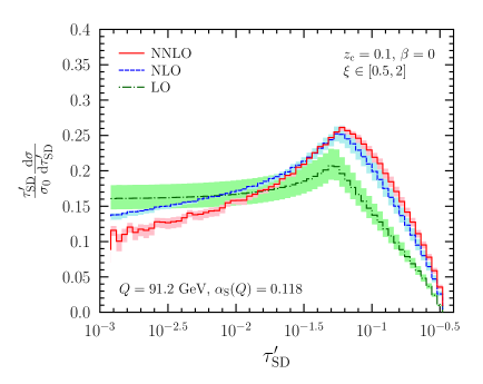
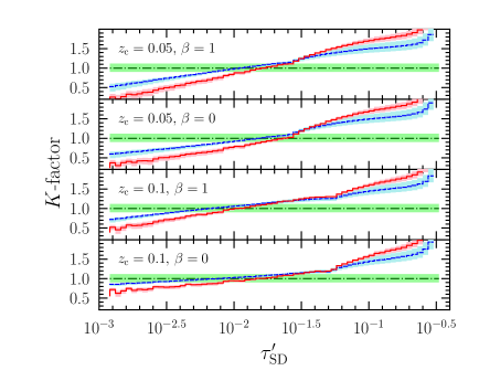
Figure 1: Predictions for the soft-drop thrust for grooming parameters $z_{\mathrm{c}}=0.1$ and $\beta=0$ at LO (dot-dashed green), NLO (dashed blue) and NNLO (solid red) accuracy (left) and $K$-factors for various $z_{\mathrm{c}}$ and $\beta$ values as indicated in the plots (left). The bands represent renormalization scale variation in the range $\xi=\mu/Q\in[0.5,2]$.

We begin the presentation of our results by considering the soft-drop thrust. Predictions for the distribution of $\tau^{\prime}_{\mathrm{SD}}=1-T^{\prime}_{\mathrm{SD}}$ for the center-of-mass energy of $Q=91.2$ GeV and grooming parameters $z_{\mathrm{c}}=0.1$ and $\beta=0$ are shown on the left panel of Figure  1 at LO (dot-dashed green), NLO (dashed blue) and NNLO (solid red) accuracy. The value of the strong coupling was chosen as $\alpha_{\mathrm{S}}(M_{Z})=0.118$. The bands correspond to varying the renormalization scale in the range $\mu\in[Q/2,2Q]$. We also present the perturbative coefficients $A_{\tau^{\prime}_{\mathrm{SD}}}$, $B_{\tau^{\prime}_{\mathrm{SD}}}$ and $C_{\tau^{\prime}_{\mathrm{SD}}}$ computed at $\mu=Q$ in Table 1 for $(z_{\mathrm{c}},\beta)=(0.1,0)$, tabulated on a linear scale in $\tau^{\prime}_{\mathrm{SD}}$. We observe the very good numerical stability of our NNLO computation over the full range of the observable considered. We have checked that this stability does not depend on the values of $z_{\mathrm{c}}$ and $\beta$.

Next, we investigate how the convergence of the perturbative prediction depends on the grooming parameters. On the right panel of Figure  1 we present the $K$-factors at NLO (dashed blue) and NNLO (solid red) as defined in Eq. (1) for four pairs of $(z_{\mathrm{c}},\beta)$ values, $\{(0.05,1),(0.05,0),(0.1,1),(0.1,0)\}$. The constant LO $K$-factor (dot-dashed green) is also shown for visual reference. In general we find that milder grooming leads to larger change from order to order in perturbation theory. Thus, grooming improves perturbative convergence as one might expect. In the ranges considered, the dependence of the $K$-factors on $\beta$ is seen to be milder than their dependence on $z_{\mathrm{c}}$. We observe that for $\tau^{\prime}_{\mathrm{SD}}\gtrsim 10^{-2}$, i.e., in the range where the bulk of the data lies, the most stable perturbative prediction is obtained for $z_{\mathrm{c}}=0.1$ and $\beta=0$.

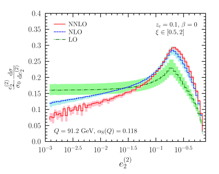
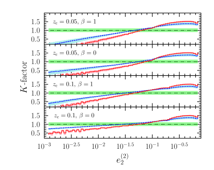
Figure 2: Predictions for the soft-drop hemisphere jet mass for grooming parameters $z_{\mathrm{c}}=0.1$ and $\beta=0$ at LO (dot-dashed green), NLO (dashed blue) and NNLO (solid red) accuracy (left) and $K$-factors for various $z_{\mathrm{c}}$ and $\beta$ values as indicated in the plots (left). The bands represent renormalization scale variation in the range $\xi=\mu/Q\in[0.5,2]$.

Turning to the soft-drop hemisphere jet mass, in Figure  2 we present our perturbative predictions for the distribution of $e_{2}^{(2)}$ at LO, NLO and NNLO accuracy for $z_{\mathrm{c}}=0.1$ and $\beta=0$ on the left panel. The $K$-factors corresponding to the same set of $(z_{\mathrm{c}},\beta)$ values as for the soft-drop thrust are shown on the right panel. We also record in Table 3 the values of the perturbative coefficients $A_{e_{2}^{(2)}}$, $B_{e_{2}^{(2)}}$ and $C_{e_{2}^{(2)}}$ computed at $\mu=Q$ for $(z_{\mathrm{c}},\beta)=(0.1,0)$, tabulated on a linear scale in $e_{2}^{(2)}$. We again observe the very good numerical stability of our NNLO predictions.

In general, we find that also for the soft-drop hemisphere jet mass, stronger grooming leads to an improved convergence of the perturbative predictions. In fact, the perturbative expansions of the distributions for soft-drop thrust and hemisphere jet mass behave very similarly with somewhat larger $K$-factors for the latter. We again find that choosing $z_{\mathrm{c}}=0.1$ and $\beta=0$ leads to the perturbatively most stable predictions.

Last, we investigate the soft-drop narrow jet mass. The fixed-order predictions for the distribution of $\rho$ at LO, NLO and NNLO are shown on the left panel of Figure  3, for jet radius $R=1$ (jets were defined using the anti-$k_{t}$ algorithm [25, 26]) and grooming parameters $z_{\mathrm{c}}=0.1$ and $\beta=0$. In Ref. [20] it was shown that the natural hard scale for this observable is $\mu=\frac{QR}{2}$, hence in Figure  3 we have set the central scale to $\mu=Q/2$. Nevertheless, in Table 2 we present the expansion coefficients $A_{\rho}$, $B_{\rho}$ and $C_{\rho}$ computed at the default renormalization scale of $\mu=Q$ for $R=1$ and $(z_{\mathrm{c}},\beta)=(0.1,0)$, tabulated on a linear scale in $\rho$. The numerical convergence of the NNLO calculation is again found to be very good.

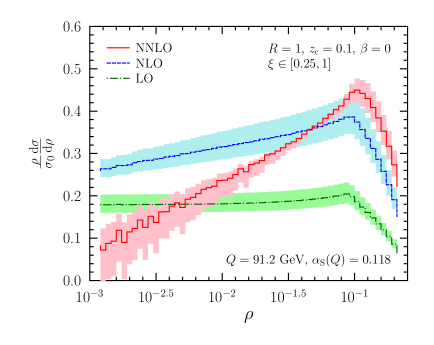
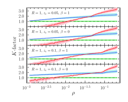
Figure 3: Predictions for the soft-drop narrow jet mass for jet radius $R=1$ and grooming parameters $z_{\mathrm{c}}=0.1$ and $\beta=0$ at LO (dot-dashed green), NLO (dashed blue) and NNLO (solid red) accuracy (left) and $K$-factors for various $z_{\mathrm{c}}$ and $\beta$ values as indicated in the plots (left). The bands represent renormalization scale variation in the range $\xi=\mu/Q\in[0.25,1]$.

Examining the $K$-factors for the narrow jet mass, shown on the left panel of Figure  3, alongside those for soft-drop thrust and hemisphere jet mass, a new feature emerges. Although stronger grooming does improve the perturbative convergence from NLO to NNLO (i.e., the ratio $K_{\rm NNLO}/K_{\rm NLO}$ is closer to unity), but the NLO $K$-factor is actually seen to increase with increasing $z_{\mathrm{c}}$ and decreasing $\beta$ (i.e., more grooming). This is readily understood from the definition of $\rho$. Since a leading-order computation involves only three massless partons in the final state, in order to obtain a narrow jet mass that is non-zero at LO requires not only that the three partons be clustered into two jets, but also that the clustering passes the soft-drop condition. Otherwise, all soft-dropped jets are massless. Starting from NLO, the extra real radiation allows for configurations where three or more partons cluster to form a single jet. Such a jet can remain massive even after the soft drop. Hence one expects that the LO contribution is reduced more by stronger grooming than higher-order corrections, leading to an increased NLO $K$-factor at larger $z_{\mathrm{c}}$ and smaller $\beta$.

We conclude that although in general grooming leads to better converging perturbative predictions, the sizes of the radiative corrections depend on the observable, being smaller for the more inclusive ones. In particular, for the narrow jet mass the NLO $K$-factor is rather large and positive (the $K$-factors are even larger for smaller jet radii), indicating that the NNLO computation represents the first reliable prediction for this quantity.

Finally, we offer a brief comment regarding all-order resummation for the observables considered here. Clearly, for small enough values of the event shapes the resummation of logarithmic contributions is mandatory. However, for soft-drop thrust and hemisphere jet mass specifically, the higher-order corrections remain moderate down to $\tau^{\prime}_{\mathrm{SD}}\simeq 10^{-3}$ and $\rho\simeq 10^{-3}$ if $z_{\mathrm{c}}=0.1$ and $\beta=0$. This suggests that the fixed-order NNLO predictions may potentially be reliable in the region with the bulk of the data (e.g., $\tau^{\prime}_{\mathrm{SD}}\gtrsim 10^{-2}$). Hence, it might be possible that resummation only becomes essential for such a small range of the shape variable, that over this range the contribution to the cross section becomes more or less negligible. As the hadronization corrections are also small for $z_{\mathrm{c}}=0.1$ and $\beta=0$ (under 10% for $\tau^{\prime}_{\mathrm{SD}}\gtrsim 10^{-2}$ [20]), the increased perturbative stability makes the soft-drop thrust and hemisphere jet mass with such grooming parameters promising event shapes for a precise determination of $\alpha_{\mathrm{S}}$, perhaps even without resummation of large logarithms.

In this letter we presented predictions for soft-drop groomed event shapes of hadronic final states in electron-positron annihilation at NNLO accuracy in perturbation theory. Our predictions for the perturbative coefficients show very good numerical stability over the complete ranges of the observables considered. We have also studied the impact of grooming on the convergence of the perturbative expansions and presented NLO and NNLO $K$-factors for several values of the grooming parameters. We observed that in general, grooming improves the perturbative convergence of the predictions. This is more pronounced for the more inclusive quantities of soft-drop thrust and hemisphere jet mass, and less so for the narrow jet mass. The increased perturbative stability, along with reduced hadronization corrections makes the soft-drop thrust and hemisphere jet mass appealing candidates for a precise determination of the strong coupling at lepton colliders.

Acknowledgments

We thank V. Theevwes for sharing the data files of the figures in Ref. [20]. A.K. acknowledges financial support from the Premium Postdoctoral Fellowship program of the Hungarian Academy of Sciences. This work was supported by grant K 125105 of the National Research, Development and Innovation Fund in Hungary.

Table 1: Perturbative coefficients for the soft-drop thrust $\tau^{\prime}_{\rm SD}$ with $(z_{\mathrm{c}},\beta)=(0.1,0)$ at $\mu=Q$. $C_{\tau^{\prime}_{\mathrm{SD}}}$ is presented only up to the kinematical limit of $B_{\tau^{\prime}_{\mathrm{SD}}}$.

$\tau^{\prime}_{\mathrm{SD}}$	$A_{\tau^{\prime}_{\mathrm{SD}}}\!\cdot\!10^{-3}$	$B_{\tau^{\prime}_{\mathrm{SD}}}\!\cdot\!10^{-4}$	$C_{\tau^{\prime}_{\mathrm{SD}}}\!\cdot\!10^{-5}$	$\tau^{\prime}_{\mathrm{SD}}$	$A_{\tau^{\prime}_{\mathrm{SD}}}\!\cdot\!10^{-3}$	$B_{\tau^{\prime}_{\mathrm{SD}}}\!\cdot\!10^{-4}$	$C_{\tau^{\prime}_{\mathrm{SD}}}\!\cdot\!10^{-5}$
$0.005$	$80.4(2)$	$-2017(4)$	$1787(4)$	$0.225$	$0.013122(3)$	$0.0447(3)$	$0.113(5)$
$0.015$	$0.62894(7)$	$0.202(2)$	$-1.34(3)$	$0.235$	$0.011427(3)$	$0.0393(3)$	$0.101(4)$
$0.025$	$0.38657(4)$	$0.249(2)$	$-0.48(3)$	$0.245$	$0.009890(2)$	$0.0363(3)$	$0.097(4)$
$0.035$	$0.28926(4)$	$0.251(2)$	$-0.11(2)$	$0.255$	$0.008492(2)$	$0.0327(3)$	$0.081(4)$
$0.045$	$0.23794(3)$	$0.234(2)$	$0.03(2)$	$0.265$	$0.007196(2)$	$0.0292(3)$	$0.079(3)$
$0.055$	$0.19907(3)$	$0.238(2)$	$0.08(2)$	$0.275$	$0.005991(2)$	$0.0263(2)$	$0.075(3)$
$0.065$	$0.15468(2)$	$0.255(2)$	$0.22(2)$	$0.285$	$0.004862(2)$	$0.0235(2)$	$0.067(3)$
$0.075$	$0.12311(2)$	$0.234(1)$	$0.32(2)$	$0.295$	$0.003791(2)$	$0.0205(2)$	$0.059(2)$
$0.085$	$0.10021(2)$	$0.2091(9)$	$0.32(2)$	$0.305$	$0.0027649(9)$	$0.0179(2)$	$0.057(2)$
$0.095$	$0.08299(2)$	$0.1877(9)$	$0.30(2)$	$0.315$	$0.0017736(8)$	$0.01478(7)$	$0.048(2)$
$0.105$	$0.069666(9)$	$0.1662(8)$	$0.31(2)$	$0.325$	$801.8(5)\!\cdot\!10^{-6}$	$0.01244(5)$	$0.0425(7)$
$0.115$	$0.059103(8)$	$0.1482(8)$	$0.28(1)$	$0.335$	$53.4(2)\!\cdot\!10^{-6}$	$0.00773(2)$	$0.0363(3)$
$0.125$	$0.050600(7)$	$0.1304(7)$	$0.26(1)$	$0.345$	$0$	$0.0025277(7)$	$0.02025(5)$
$0.135$	$0.043611(6)$	$0.1167(6)$	$0.227(9)$	$0.355$	$0$	$0.0012796(3)$	$0.01016(3)$
$0.145$	$0.037822(6)$	$0.1043(6)$	$0.228(8)$	$0.365$	$0$	$680.7(3)\!\cdot\!10^{-6}$	$0.00557(2)$
$0.155$	$0.032941(5)$	$0.0925(6)$	$0.209(8)$	$0.375$	$0$	$356.9(2)\!\cdot\!10^{-6}$	$0.00301(1)$
$0.165$	$0.028799(5)$	$0.0839(5)$	$0.181(7)$	$0.385$	$0$	$177.5(1)\!\cdot\!10^{-6}$	$0.001576(6)$
$0.175$	$0.025239(4)$	$0.0749(5)$	$0.163(7)$	$0.395$	$0$	$79.04(7)\!\cdot\!10^{-6}$	$767(4)\!\cdot\!10^{-6}$
$0.185$	$0.022159(4)$	$0.0668(4)$	$0.153(6)$	$0.405$	$0$	$28.19(4)\!\cdot\!10^{-6}$	$328(2)\!\cdot\!10^{-6}$
$0.195$	$0.019465(4)$	$0.0604(4)$	$0.141(6)$	$0.415$	$0$	$5.21(2)\!\cdot\!10^{-6}$	$102.3(7)\!\cdot\!10^{-6}$
$0.205$	$0.017095(3)$	$0.0540(4)$	$0.130(6)$	$0.425$	$0$	$2.6(2)\!\cdot\!10^{-9}$	$6.6(2)\!\cdot\!10^{-6}$
$0.215$	$0.014994(3)$	$0.0494(4)$	$0.116(5)$

Table 2: Perturbative coefficients for the narrow jet mass $\rho$ with $R=1$ and $(z_{\mathrm{c}},\beta)=(0.1,0)$ at $\mu=Q$. $C_{\rho}$ is presented only up to the kinematical limit of $B_{\rho}$.

$\rho$	$A_{\rho}\cdot 10^{-3}$	$B_{\rho}\cdot 10^{-4}$	$C_{\rho}\cdot 10^{-5}$	$\rho$	$A_{\rho}\cdot 10^{-3}$	$B_{\rho}\cdot 10^{-4}$	$C_{\rho}\cdot 10^{-5}$
$0.005$	$174.8(5)$	$-2492(5)$	$2415(4)$	$0.195$	$0.022163(7)$	$0.1384(2)$	$0.613(5)$
$0.015$	$0.6028(2)$	$2.555(2)$	$-2.25(5)$	$0.205$	$0.018671(6)$	$0.1194(2)$	$0.550(4)$
$0.025$	$0.35799(7)$	$1.601(2)$	$0.02(4)$	$0.215$	$0.015404(5)$	$0.1017(2)$	$0.473(4)$
$0.035$	$0.25785(5)$	$1.1847(9)$	$0.62(3)$	$0.225$	$0.012191(5)$	$0.0855(1)$	$0.419(3)$
$0.045$	$0.20315(4)$	$0.9489(7)$	$0.86(3)$	$0.235$	$0.008854(4)$	$0.07012(8)$	$0.356(3)$
$0.055$	$0.16856(4)$	$0.7945(7)$	$0.99(2)$	$0.245$	$0.004583(3)$	$0.05802(5)$	$0.307(2)$
$0.065$	$0.14480(3)$	$0.6863(6)$	$1.03(2)$	$0.255$	$0$	$0.033405(8)$	$0.2442(7)$
$0.075$	$0.12755(3)$	$0.6061(6)$	$1.06(2)$	$0.265$	$0$	$0.014268(4)$	$0.1290(3)$
$0.085$	$0.11445(3)$	$0.5445(5)$	$1.05(2)$	$0.275$	$0$	$0.007721(3)$	$0.0734(2)$
$0.095$	$0.09988(3)$	$0.5029(5)$	$1.18(2)$	$0.285$	$0$	$0.004371(2)$	$0.0437(2)$
$0.105$	$0.08443(2)$	$0.4521(4)$	$1.25(2)$	$0.295$	$0$	$0.002488(2)$	$0.0257(1)$
$0.115$	$0.07200(2)$	$0.3995(4)$	$1.22(1)$	$0.305$	$0$	$0.0013994(8)$	$0.01518(7)$
$0.125$	$0.06184(2)$	$0.3519(4)$	$1.175(9)$	$0.315$	$0$	$766.6(6)\!\cdot\!10^{-6}$	$0.00873(5)$
$0.135$	$0.05340(2)$	$0.3091(3)$	$1.099(8)$	$0.325$	$0$	$393.7(4)\!\cdot\!10^{-6}$	$0.00489(3)$
$0.145$	$0.04624(2)$	$0.2718(3)$	$1.016(8)$	$0.335$	$0$	$177.5(3)\!\cdot\!10^{-6}$	$0.00251(2)$
$0.155$	$0.04012(1)$	$0.2391(3)$	$0.930(7)$	$0.345$	$0$	$63.1(2)\!\cdot\!10^{-6}$	$0.00111(1)$
$0.165$	$0.034803(9)$	$0.2095(2)$	$0.850(6)$	$0.355$	$0$	$12.47(6)\!\cdot\!10^{-6}$	$326(4)\!\cdot\!10^{-6}$
$0.175$	$0.030127(8)$	$0.1834(2)$	$0.775(6)$	$0.365$	$0$	$26(2)\!\cdot\!10^{-9}$	$16.3(6)\!\cdot\!10^{-6}$
$0.185$	$0.025951(8)$	$0.1599(2)$	$0.686(5)$

Table 3: Perturbative coefficients for the hemisphere jet mass $e_{2}^{(2)}$ with $(z_{\mathrm{c}},\beta)=(0.1,0)$ at $\mu=Q$. $C_{e_{2}^{(2)}}$ is presented only up to the kinematical limit of $B_{e_{2}^{(2)}}$.

$e_{2}^{(2)}$	$A_{e_{2}^{(2)}}\!\cdot\!10^{-3}$	$B_{e_{2}^{(2)}}\!\cdot\!10^{-4}$	$C_{e_{2}^{(2)}}\!\cdot\!10^{-5}$	$e_{2}^{(2)}$	$A_{e_{2}^{(2)}}\!\cdot\!10^{-3}$	$B_{e_{2}^{(2)}}\!\cdot\!10^{-4}$	$C_{e_{2}^{(2)}}\!\cdot\!10^{-5}$
$0.005$	$79.2(2)$	$-2016(4)$	$1792(4)$	$0.425$	$0.017936(4)$	$0.03617(4)$	$0.064(3)$
$0.015$	$0.6040(2)$	$-0.1789(8)$	$-2.31(4)$	$0.435$	$0.017151(4)$	$0.03477(4)$	$0.059(3)$
$0.025$	$0.35912(7)$	$-0.0177(5)$	$-1.14(3)$	$0.445$	$0.016391(4)$	$0.03330(4)$	$0.056(3)$
$0.035$	$0.25908(5)$	$0.0304(4)$	$-0.70(2)$	$0.455$	$0.015674(4)$	$0.03190(4)$	$0.054(3)$
$0.045$	$0.20438(4)$	$0.0507(4)$	$-0.44(2)$	$0.465$	$0.014986(4)$	$0.03060(4)$	$0.054(3)$
$0.055$	$0.16982(4)$	$0.0615(3)$	$-0.35(2)$	$0.475$	$0.014334(3)$	$0.02924(3)$	$0.049(2)$
$0.065$	$0.14617(3)$	$0.0677(3)$	$-0.22(2)$	$0.485$	$0.013701(3)$	$0.02801(3)$	$0.048(2)$
$0.075$	$0.12900(3)$	$0.0724(3)$	$-0.18(2)$	$0.495$	$0.013093(3)$	$0.02679(3)$	$0.048(2)$
$0.085$	$0.11589(3)$	$0.0750(2)$	$-0.12(2)$	$0.505$	$0.012514(3)$	$0.02554(3)$	$0.045(2)$
$0.095$	$0.10574(3)$	$0.0776(2)$	$-0.09(2)$	$0.515$	$0.011953(3)$	$0.02441(3)$	$0.041(2)$
$0.105$	$0.09752(2)$	$0.0793(2)$	$-0.05(2)$	$0.525$	$0.011408(3)$	$0.02327(3)$	$0.039(2)$
$0.115$	$0.09083(2)$	$0.0808(2)$	$-0.007(10)$	$0.535$	$0.010884(3)$	$0.02207(3)$	$0.038(2)$
$0.125$	$0.08536(2)$	$0.0816(2)$	$-0.013(10)$	$0.545$	$0.010370(3)$	$0.02093(2)$	$0.035(2)$
$0.135$	$0.08073(2)$	$0.0828(2)$	$0.021(9)$	$0.555$	$0.009869(3)$	$0.01985(2)$	$0.032(2)$
$0.145$	$0.07688(2)$	$0.0832(2)$	$0.030(9)$	$0.565$	$0.009390(3)$	$0.01875(2)$	$0.033(2)$
$0.155$	$0.07358(2)$	$0.0833(2)$	$0.052(8)$	$0.575$	$0.008911(2)$	$0.01764(2)$	$0.030(2)$
$0.165$	$0.07082(2)$	$0.0828(2)$	$0.042(8)$	$0.585$	$0.008449(2)$	$0.01657(2)$	$0.028(2)$
$0.175$	$0.06845(2)$	$0.0817(2)$	$0.070(8)$	$0.595$	$0.007992(2)$	$0.01554(2)$	$0.024(2)$
$0.185$	$0.06643(2)$	$0.0781(2)$	$0.036(8)$	$0.605$	$0.007538(2)$	$0.01450(2)$	$0.022(1)$
$0.195$	$0.06320(2)$	$0.0783(2)$	$0.049(8)$	$0.615$	$0.007089(2)$	$0.01344(2)$	$0.021(1)$
$0.205$	$0.05874(2)$	$0.0808(2)$	$0.071(7)$	$0.625$	$0.006643(2)$	$0.01244(2)$	$0.0207(9)$
$0.215$	$0.05478(2)$	$0.0802(2)$	$0.079(7)$	$0.635$	$0.006192(2)$	$0.01146(2)$	$0.0175(8)$
$0.225$	$0.05119(2)$	$0.0788(2)$	$0.083(7)$	$0.645$	$0.005746(2)$	$0.01046(2)$	$0.0153(8)$
$0.235$	$0.04797(1)$	$0.0768(2)$	$0.103(6)$	$0.655$	$0.005296(2)$	$0.00948(2)$	$0.0141(7)$
$0.245$	$0.04505(1)$	$0.0743(1)$	$0.099(6)$	$0.665$	$0.004830(2)$	$0.00850(1)$	$0.0117(7)$
$0.255$	$0.042376(9)$	$0.07180(9)$	$0.094(6)$	$0.675$	$0.004359(2)$	$0.00752(1)$	$0.0105(6)$
$0.265$	$0.039926(9)$	$0.06926(9)$	$0.092(6)$	$0.685$	$0.003874(2)$	$0.006593(9)$	$0.0083(5)$
$0.275$	$0.037697(8)$	$0.06666(8)$	$0.097(5)$	$0.695$	$0.003369(2)$	$0.005645(8)$	$0.0073(5)$
$0.285$	$0.035639(8)$	$0.06417(8)$	$0.097(5)$	$0.705$	$0.002843(1)$	$0.004749(7)$	$0.0061(4)$
$0.295$	$0.033751(7)$	$0.06167(8)$	$0.099(5)$	$0.715$	$0.0022871(9)$	$0.003931(6)$	$0.0056(4)$
$0.305$	$0.031981(7)$	$0.05915(7)$	$0.088(5)$	$0.725$	$0.0016951(7)$	$0.003205(5)$	$0.0046(3)$
$0.315$	$0.030343(7)$	$0.05690(7)$	$0.089(5)$	$0.735$	$0.0010592(6)$	$0.002754(4)$	$0.0044(2)$
$0.325$	$0.028826(7)$	$0.05464(6)$	$0.087(4)$	$0.745$	$367.5(4)\!\cdot\!10^{-6}$	$0.002889(2)$	$0.0051(1)$
$0.335$	$0.027407(6)$	$0.05245(6)$	$0.077(4)$	$0.755$	$0$	$0.0018054(7)$	$0.00524(3)$
$0.345$	$0.026087(6)$	$0.05042(6)$	$0.092(4)$	$0.765$	$0$	$751.8(3)\!\cdot\!10^{-6}$	$0.00248(2)$
$0.355$	$0.024841(5)$	$0.04837(6)$	$0.076(4)$	$0.775$	$0$	$380.1(2)\!\cdot\!10^{-6}$	$0.001189(9)$
$0.365$	$0.023668(5)$	$0.04642(5)$	$0.076(4)$	$0.785$	$0$	$191.1(2)\!\cdot\!10^{-6}$	$581(5)\!\cdot\!10^{-6}$
$0.375$	$0.022574(5)$	$0.04445(5)$	$0.081(4)$	$0.795$	$0$	$89.11(8)\!\cdot\!10^{-6}$	$255(3)\!\cdot\!10^{-6}$
$0.385$	$0.021545(5)$	$0.04283(5)$	$0.071(3)$	$0.805$	$0$	$35.65(5)\!\cdot\!10^{-6}$	$99(2)\!\cdot\!10^{-6}$
$0.395$	$0.020570(5)$	$0.04100(5)$	$0.073(3)$	$0.815$	$0$	$10.24(3)\!\cdot\!10^{-6}$	$29.5(8)\!\cdot\!10^{-6}$
$0.405$	$0.019638(5)$	$0.03928(5)$	$0.067(3)$	$0.825$	$0$	$1.241(8)\!\cdot\!10^{-6}$	$1.6(2)\!\cdot\!10^{-6}$
$0.415$	$0.018760(4)$	$0.03781(4)$	$0.063(3)$	$0.835$	$0$	$2.3(2)\!\cdot\!10^{-9}$	$139(4)\!\cdot\!10^{-9}$

References

• [1] G. Degrassi, S. Di Vita, J. Elias-Miro, J. R. Espinosa, G. F. Giudice, G. Isidori, A. Strumia, JHEP 1208 (2012) 098.
• [2] S. Brandt, C. Peyrou, R. Sosnowski, A. Wroblewski, Phys. Lett. 12 (1964) 57.
• [3] E. Farhi, Phys. Rev. Lett. 39 (1977) 1587.
• [4] A. Gehrmann-De Ridder, T. Gehrmann, E. W. N. Glover, G. Heinrich, JHEP 0712 (2007) 094.
• [5] S. Weinzierl, JHEP 0906 (2009) 041.
• [6] V. Del Duca, C. Duhr, A. Kardos, G. Somogyi, Z. Trócsányi, Phys. Rev. Lett. 117 (2016) no.15, 152004.
• [7] V. Del Duca, C. Duhr, A. Kardos, G. Somogyi, Z. Szőr, Z. Trócsányi, Z. Tulipánt, Phys. Rev. D 94 (2016) no.7, 074019.
• [8] T. Becher, M. D. Schwartz, JHEP 0807 (2008) 034.
• [9] J. M. Butterworth, A. R. Davison, M. Rubin, G. P. Salam, Phys. Rev. Lett.  100 (2008) 242001.
• [10] D. Krohn, J. Thaler, L.-T. Wang, JHEP 1002 (2010) 084.
• [11] S. D. Ellis, C. K. Vermilion, J. R. Walsh, Phys. Rev. D 80 (2009) 051501.
• [12] S. D. Ellis, C. K. Vermilion, J. R. Walsh, Phys. Rev. D 81 (2010) 094023.
• [13] M. Dasgupta, A. Fregoso, S. Marzani, G. P. Salam, JHEP 1309 (2013) 029.
• [14] A. J. Larkoski, S. Marzani, G. Soyez, J. Thaler, JHEP 1405 (2014) 146.
• [15] C. Frye, A. J. Larkoski, M. D. Schwartz, K. Yan, JHEP 1607 (2016) 064.
• [16] C. Frye, A. J. Larkoski, M. D. Schwartz, K. Yan, arXiv:1603.06375 [hep-ph].
• [17] S. Marzani, L. Schunk, G. Soyez, JHEP 1707 (2017) 132.
• [18] S. Marzani, L. Schunk, G. Soyez, Eur. Phys. J. C 78 (2018) no.2, 96.
• [19] Z.-B. Kang, K. Lee, X. Liu, F. Ringer, arXiv:1803.03645 [hep-ph].
• [20] J. Baron, S. Marzani, V. Theeuwes, arXiv:1803.04719 [hep-ph].
• [21] O. V. Tarasov, A. A. Vladimirov, A. Yu. Zharkov, Phys. Lett. B 93 (1980) 429.
• [22] Z. Tulipánt, A. Kardos, G. Somogyi, Eur. Phys. J. C 77 (2017) no.11, 749.
• [23] G. Somogyi, Z. Trócsányi, V. Del Duca, JHEP 0701 (2007) 070.
• [24] G. Somogyi, Z. Trócsányi, JHEP 0701 (2007) 052.
• [25] M. Cacciari, G. P. Salam, G. Soyez, JHEP 0804 (2008) 063.
• [26] M. Cacciari, G. P. Salam, G. Soyez, Eur. Phys. J. C 72 (2012) 1896.