$E$ and $B$ polarizations from inhomogeneous and solar surface turbulence

Abstract

Gradient- and curl-type or $E$- and $B$-type polarizations have been routinely analyzed to study the physics contributing to the cosmic microwave background polarization and galactic foregrounds. They characterize the parity-even and parity-odd properties of the underlying physical mechanisms, for example hydromagnetic turbulence in the case of dust polarization. Here we study spectral correlation functions characterizing the parity-even and parity-odd parts of linear polarization for homogeneous and inhomogeneous turbulence to show that only the inhomogeneous helical case can give rise to a parity-odd polarization signal. We also study nonhelical turbulence and suggest that a strong nonvanishing (here negative) skewness of the $E$ polarization is responsible for an enhanced ratio of the $EE$ to the $BB$ (quadratic) correlation in both helical and nonhelical cases. This could explain the enhanced $EE/BB$ ratio observed recently for dust polarization. We close with a preliminary assessment of using linear polarization of the Sun to characterize its helical turbulence without being subjected to the $\pi$ ambiguity that magnetic inversion techniques have to address.

,

1. Introduction

Helicity characterizes the swirl of a flow or a magnetic field. Examples include the cyclonic and anticyclonic flows on a weathermap, which are systematically different in the northern and southern hemispheres. Similar differences are also seen on the solar surface, where both flow and magnetic field vectors show swirl. Both fields play important roles in the solar dynamo, which is believed to be responsible for the generation of the Sun’s large-scale magnetic field (Moffatt, 1978; Krause & Rädler, 1980; Brandenburg & Subramanian, 2005).

To determine the solar magnetic helicity, one first needs to determine the magnetic field $\bm{b}$. This is done by measuring all four Stokes parameters to compute $\bm{b}$ at the visible surface. Historically, the first evidence for a helical magnetic field came from estimates of the mean current helicity density, $\langle\bm{j}\cdot\bm{b}\rangle$, where $\bm{j}={\bm{\nabla}}\times\bm{b}/\mu_{0}$ is the current density and $\mu_{0}$ is the vacuum permeability. Under the assumption of isotropy, using local Cartesian coordinates, we have $\langle\bm{j}\cdot\bm{b}\rangle\approx\langle j_{z}b_{z}\rangle/3$, where $j_{z}=(\partial_{x}B_{y}-\partial_{y}B_{x})/\mu_{0}$ is the vertical component of the current density, which involves only horizontal derivatives. Another approach is to assume that the magnetic field above the solar surface is nearly force-free. A vanishing Lorentz force ($\bm{j}\times\bm{b}=\bm{0}$) implies that $\bm{j}$ is parallel to $\bm{b}$, so $j_{z}=\alpha b_{z}/\mu_{0}$ with some coefficient $\alpha$. The sign of $\alpha$ is directly related to the sign of the local current helicity density. Seehafer (1990) and Pevtsov et al. (1995) computed $\alpha$ and found it to be negative in the northern hemisphere and positive in the southern. This is a statistical result that has been confirmed many times since then; see e.g., Singh et al. (2018).

A general difficulty in determining magnetic helicity lies in the fact that the horizontal magnetic field components are only determined up to the $\pi$ ambiguity. In other words, one only measures horizontal magnetic field vectors without arrow heads. The actual horizontal field direction is usually “reconstructed” by comparing with that expected from a potential magnetic field extrapolation, which only depends on the vertical magnetic field. It is unclear to what extent this assumption introduces errors and how those affect, for example, the scale dependence of the magnetic helicity that was determined in some of the aforementioned approaches (see, e.g., Zhang et al., 2014, 2016; Brandenburg et al., 2017; Singh et al., 2018).

To address the question about the limitations resulting from the $\pi$ ambiguity, we study here another potential proxy of magnetic helicity that is independent of the $\pi$ ambiguity. To this end, we decompose Stokes $Q$ and $U$, which characterize linear polarization, into the $E$ and $B$ polarizations that are routinely used in the cosmological context (Kamionkowski et al., 1997a; Seljak & Zaldarriaga, 1997) as polarized emission from the cosmic microwave background (CMB). The $E$ and $B$ polarizations characterize parity-even and parity-odd contributions; see Kamionkowski & Kosowsky (1999) for a review. In the CMB, correlations of $B$ polarization with parity-even quantities such as intensity, temperature, or the $E$ polarization are believed to be proxies of the helicity of the underlying magnetic field (Kahniashvili et al., 2014).

Observations of $E$ and $B\,$ polarizations have been obtained at various frequencies using the Planck satellite. Much of the $B$ polarization is now believed to come from the galactic foregrounds including gravitational lensing, for example. While a definitive $EB$ cross correlation has not yet been detected, we do know that the $EE$ correlation is about twice as large as the $BB$ correlation in the diffuse emission (Planck Collaboration Int. XXX, 2016). This was unexpected at the time (Caldwell et al., 2017) and will also be addressed in this paper.

Kritsuk et al. (2018) have shown that supersonic hydromagnetic turbulent star formation simulations are able to reproduce the observed $EE/BB$ ratio of about two, but the physical reason for this was not identified. Kandel et al. (2017) discussed the dominance of magnetic over kinetic energy density as an important contributor for causing the enhanced ratio. Here, instead, we identify a strong skewness of the intrinsic $E$ polarization at all depths along the line of sight as an important factor.

Our main objective is to study the connection between $EB$ cross correlation and magnetic or kinetic helicities in various turbulent flows, which can be related to what happens at the surface of the Sun. As we will show in this paper, such a connection exists only under certain inhomogeneous conditions, for example in the proximity of a surface above the solar convection zone. This automatically gives preference to one over the other viewing direction of the plane perpendicular to the line of sight. In homogeneous turbulence, by contrast, there is no way of differentiating one viewing direction from the other.

Figure 1.— Sketch illustrating the same shape of streamlines for updrafts and downdrafts for convection in the northern hemisphere ($\bm{g}\cdot\bm{\Omega}<0$), as viewed from top down.

Certain physical circumstances may well give preference to one over the other side of a plane. The CMB may indeed be one such example. Rotating stratified convection is another rather intuitive example, as illustrated in Figure 1. In this sketch one sees the flow lines of cyclonic convection around down- and upflows in the northern hemisphere as viewed from the top, so all converging inflows attain a counterclockwise swirl, and all diverging outflows attain a clockwise swirl. As seen from the sketch, however, the orientations of both flow patterns consisting of unsigned flow lines is the same. This curl-type pattern gives rise to $B$-type polarization of positive sign (e.g. Kahniashvili et al., 2014), as will be verified in the next section. It is only if we were to flip this plane or when inspecting this pattern from beneath that we will see a mirror image of the original pattern and therefore the opposite sign of the $B$ polarization; see Durrer (2008). Here, the $E$ polarization is the same when viewed from beneath (or in a mirror). This gives rise to a systematic $EB$ correlation. The $E$ polarization will also be positive in this case if a ring-like pattern dominates over a star-like pattern. This results in a positive $EB$ correlation in the north and negative in the south.

The purpose of this work is to use various numerical simulations to determine the relation between magnetic helicity and the $EB$ correlation that is derived from just the horizontal field vectors without knowledge of which of the two horizontal directions the vector points into (i.e., the $\pi$ ambiguity). The simulations include decaying homogeneous helical and nonhelical turbulence and rotating stratified convection, which can serve as a prototype for convective turbulence at the solar surface.

2. $E$ and $B$ polarization

2.1. Formalism

We consider magnetic field vectors, $\bm{b}=(b_{x},b_{y},b_{z})$, in one or several two-dimensional $xy$ cross-sections in a three-dimensional volume. We assume that this magnetic field affects the polarization of the electromagnetic radiation whose electric field vectors in the $(x,y)$ plane are $\mbox{\boldmath$e$}{}=(e_{x},e_{y})$. It is convenient to use complex notation and write this vector as $e_{x}+{\rm i}e_{y}\equiv|e|\,\exp({\rm i}\psi_{e})$, where $\psi_{e}$ is the angle of the electric field with the $x$ axis. Likewise, we write the magnetic field in the plane, $(b_{x},b_{y})$, as $b_{x}+{\rm i}b_{y}\equiv|b|\,\exp({\rm i}\psi_{b})$. For electromagnetic radiation, electric and magnetic field vectors are at right angles to each other, so $\psi_{e}=\psi_{b}+\pi/2$. In complex form, the intrinsic (or local) polarization $p(x,y,z)$ is proportional to the square of the complex electric field, i.e., $p\propto(e_{x}+{\rm i}e_{y})^{2}\propto-\epsilon\,(b_{x}+{\rm i}b_{y})^{2}$, where $\epsilon(x,y,z)$ is the local emissivity. The magnetic field of the electromagnetic radiation aligns with the ambient magnetic field, so that

$$p=-\epsilon\,(b_{x}+{\rm i}b_{y})^{2}/\bm{b}^{2}.$$ (1)

In most of the cases, we assume $\epsilon\propto\bm{b}^{2}$, which would be appropriate for the Sun (Skumanich & Lites, 1987; Bai et al., 2014). For dust polarization, on the other hand, we assume $\epsilon$ to be independent of $|\bm{b}|$; see Planck Collaboration Int. XX (2015) and Bracco et al. (2018) for details. The observable complex polarization, $P=Q+{\rm i}U$, is the line-of-sight integral

$$P(x,y)=\int p(x,y,z)\,e^{-\tau(x,y,z)}\,{\rm d}{}z,$$ (2)

with $\tau(x,y,z)$ being the optical depth with respect to the observer. If the medium can be considered optically thin, as for diffuse dust emission in the interstellar medium, we can set $\tau=0$. This will also be done in the present work. In addition, we study the polarization from individual slices, which corresponds to an optically thick case for that slice.

Next, we define $R=E+{\rm i}B$, where $E$ and $B$ are the parity even and parity odd contributions to the complex polarization, respectively. They are related to each other in Fourier space via (Seljak & Zaldarriaga, 1997; Kamionkowski et al., 1997a, b; Kamionkowski & Kovetz, 2016)

$$\tilde{R}(k_{x},k_{y})=(\hat{k}_{x}-{\rm i}\hat{k}_{y})^{2}\tilde{P}(k_{x},k_{y}),$$ (3)

where $\hat{k}_{x}$ and $\hat{k}_{y}$ are the $x$ and $y$ components of the planar unit vector $\hat{\bm{k}}=\bm{k}/k$, with $\bm{k}=(k_{x},k_{y})$ and $k=(k_{x}^{2}+k_{y}^{2})^{1/2}$ being the length of $\bm{k}$. Tildes indicate Fourier transformation over $x$ and $y$. We transform $\tilde{R}$ back into real space to obtain $E(x,y)$ and $B(x,y)$ at a given position $z$. We plot contours of $E$ and $B$ and overplot polarization vectors with angles

$$\chi_{E}={\textstyle{1\over 2}}\arg P_{E}\quad\mbox{and}\quad\chi_{B}={\textstyle{1\over 2}}\arg P_{B},$$ (4)

where $P_{E}$ and $P_{B}$ are computed in Fourier space as $\hat{P}_{E}=(\hat{k}_{x}+{\rm i}\hat{k}_{y})^{2}\tilde{E}$ and $\hat{P}_{B}=(\hat{k}_{x}+{\rm i}\hat{k}_{y})^{2}({\rm i}\tilde{B})$.

We consider shell-integrated spectra along a ring of radius $k=|\bm{k}|$ in wavenumber space of the form

$$C_{XY}(k)=\int_{0}^{2\pi}\tilde{X}(\bm{k})\,\tilde{Y}^{*}(\bm{k})\,k\,{\rm d}{}\phi_{k},$$ (5)

where $\phi_{k}$ is the azimuthal angle in Fourier space, and $\tilde{X}$ and $\tilde{Y}$ are Fourier transformed fields that each (or both) stand for $\tilde{E}$ or $\tilde{B}$. Thus, we consider the spectra $C_{EE}(k)$, $C_{EB}(k)$, and $C_{BB}(k)$. In some cases, we consider one-point correlators, which are equal to the integrated spectrum, i.e., $\langle XY\rangle_{xy}=\int C_{XY}(k)\,{\rm d}{}k$. In the following, when we sometimes talk about $EE$ or $BB$ correlations, we always mean the spectral correlation functions $C_{EE}(k)$ and $C_{BB}(k)$.

2.2. Two-scale analysis

In the Sun, we expect opposite signs of the $EB$ correlation in the northern and southern hemispheres. An analogous situation has been encountered previously in connection with magnetic helicity measurements. To prevent cancelation from contributions of opposite signs coming systematically from the two hemispheres, one has to allow for a corresponding modulation of the sign between the hemispheres. We refer here to the work of Roberts & Soward (1975) for the general formalism in the context of dynamo theory and to Brandenburg et al. (2017) for the application to observational data similar to those discussed here. The two-scale formalism has so far only been developed for Cartesian geometry, but it is conceivable that it can also be extended to spherical harmonics.

Here we assume that the $x$ direction points in longitude and the $y$ direction points in latitude. To account for a sinusoidal modulation in latitude proportional to $\sin K_{y}y$, we compute the following generalized spectrum as

$$C_{XY}(\bm{K},k)=\int_{0}^{2\pi}\tilde{X}(\bm{k}+{\textstyle{1\over 2}}\bm{K})\,\tilde{Y}^{*}(\bm{k}-{\textstyle{1\over 2}}\bm{K})\,k\,{\rm d}{}\phi_{k},$$ (6)

and plot $-\mbox{\rm Im}\,C_{XY}(\bm{K},k)$ versus $k$ for $\bm{K}=(0,K_{y})$; see also Singh et al. (2018) and Zhang & Brandenburg (2018) for recent applications.

2.3. A simple example

We consider gradient- and curl-type vector fields (Durrer, 2008)

$$F_{i}(x,y)=\partial_{i}f,\quad G_{i}(x,y)=\epsilon_{ij}\partial_{j}g,$$ (7)

using

$$f=f_{0}\cos kx\cos ky,\quad g=g_{0}\cos kx\cos ky.$$ (8)

The two-dimensional projection of an otherwise three-dimensional magnetic field in this model is given by $\bm{b}(x,y)=\bm{F}+\mbox{\boldmath$G$}{}$. Here, $\epsilon_{ij}$ is the totally antisymmetric tensor in two dimensions, so $\epsilon_{12}=1$, $\epsilon_{21}=-1$, and zero otherwise. Assuming $k=1$ in a domain $-\pi<(x,y)<\pi$, we have

$$\bm{F}=-f_{0}\pmatrix{\sin x\cos y\cr\cos x\sin y},\quad\mbox{\boldmath$G$}{}=g_{0}\pmatrix{-\cos x\sin y\cr+\sin x\cos y}.$$ (9)

In Figure 2 we show examples of polarization maps for different combinations of the coefficients $(f_{0},g_{0})$. The polarization vectors correspond to $\bm{b}$ vectors without an arrow. Pure $E$ polarization occurs whenever either $f_{0}$ or $g_{0}$ vanish, whereas pure $B$ polarization occurs whenever $|f_{0}|=|g_{0}|$. Thus, there is no direct correspondence between gradient- and curl-type vector fields and gradient- and curl-type polarization. Thus, Equation (5.84) of Durrer (2008) is incorrect (R. Durrer, private communication).

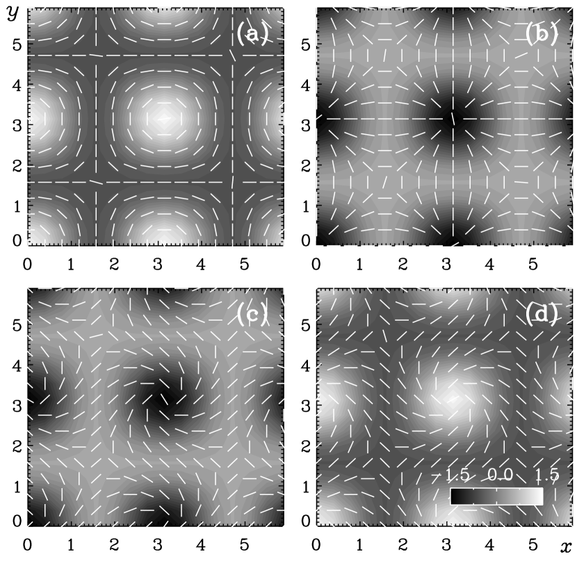
Figure 2.— (a) and (b): pure $E$ polarization for cases $(f_{0},g_{0})=(1,0)$ and $(0,1)$, respectively. (c) and (d): pure B polarization for cases $(f_{0},g_{0})=(1,\pm 1)$, for upper and lower signs, respectively.

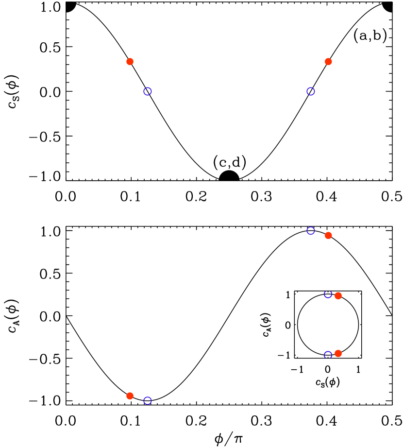
Figure 3.— Dependence of real-space correlations $c_{\rm S}(\phi)$ (top) and $c_{\rm A}(\phi)$ (bottom) on $\phi$. The inset shows a parametric representation of $c_{\rm A}(\phi)$ versus $c_{\rm S}(\phi)$. The open blue and filled red symbols denote the points where $\langle E^{2}\rangle/\langle B^{2}\rangle=1$ and $2$, respectively. The black filled symbols denote the examples of pure $E$ polarizations in Figure 2(a+b) and pure $B$ polarizations in Figure 2(c+d).

It is convenient to define normalized symmetric and antisymmetric polarization correlations as

$$c_{\rm S}=\langle E^{2}-B^{2}\rangle\left/\langle E^{2}+B^{2}\rangle\right.$$ (10)

and

$$c_{\rm A}=2\langle EB\rangle\left/\langle E^{2}+B^{2}\rangle\right.$$ (11)

and display them as a function of $\phi$ with $(f_{0},g_{0})=(\cos\phi,\sin\phi)$. Here angle brackets denote averaging over the $xy$ plane. The resulting polarization maps are shown in Figure 3. In this model, the points in a parametric representation of $c_{\rm A}$ versus $c_{\rm S}$ lie on a closed, nearly circular line; see the inset of Figure 3.

Pure $E$ polarization implies $c_{\rm S}=1$, while pure $B$ polarization implies $c_{\rm S}=-1$. In both cases, we have $c_{\rm A}=0$. Furthermore, the case $c_{\rm S}=0$ (which coincides with $c_{\rm A}=\pm 1$) corresponds to $\langle E^{2}\rangle/\langle B^{2}\rangle=1$. This is what was theoretically expected in the case of dust polarization as a probe of ISM turbulence; see Caldwell et al. (2017). However, of particular interest is now the case $\langle E^{2}\rangle/\langle B^{2}\rangle=2$, which has been detected in foreground polarization with Planck (Planck Collaboration Int. XXX, 2016; Planck Collaboration results XI, 2018). In our model, this implies $c_{\rm S}=1/3$ with $c_{\rm A}=\pm 2\sqrt{2}/3$.

Analogously to the real-space coefficients $c_{\rm S}=0$ and $c_{\rm A}=0$, we define normalized spectra as

$$c_{\rm S}(k)={C_{EE}(k)-C_{BB}(k)\over C_{EE}(k)+C_{BB}(k)}$$ (12)

and

$$c_{\rm A}(k)={2C_{EB}(k)\over C_{EE}(k)+C_{BB}(k)}.$$ (13)

Unless noted otherwise $E$ and $B$ have been obtained from simulations through integration along the $z$ direction; see Equation (2).

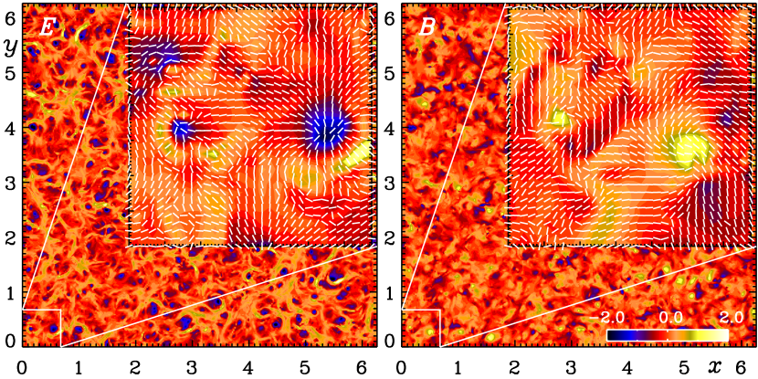
Figure 4.— $E$-mode (left) and $B$-mode (right) polarization for isotropic fully helical magnetohydrodynamic turbulence using an $xy$ slice of $E$ and $B$ from Brandenburg & Kahniashvili (2017) (their Figures 4d–f, for $\mbox{\rm Pr}_{M}=100$). Dark (light) shades indicate negative (positive) velocity. In each panel, the insets show an enlarged portion where we also show the $E$ and $B$ polarization vectors.

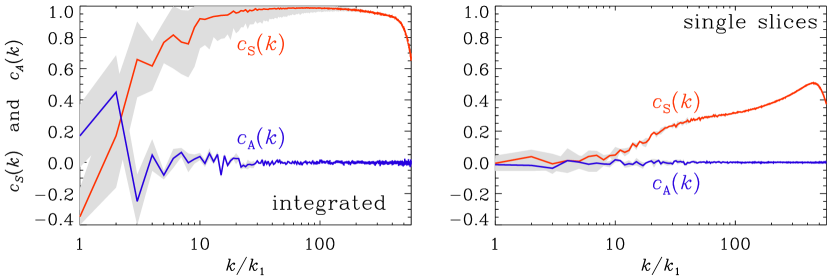
Figure 5.— Spectral correlation functions $c_{\rm S}(k)$ and $c_{\rm A}(k)$ using line-of-sight integrated polarization (left) and single slice data (right) computed from decaying isotropic turbulence of Brandenburg & Kahniashvili (2017). Error margins are indicated in gray.

3. Numerical simulations

3.1. Isotropic turbulence simulations

Astrophysical turbulence comes in a multitude of different forms: it can be helical or nonhelical, it can be magnetically dominated or subdominant, it can possess cross helicity, with a systematic alignment. These turbulence simulations provide a means of performing experiments in a variety of circumstances and environments. Here we use three-dimensional simulation data of isotropic MHD turbulence and consider separately all $xy$ planes. The simulations describe decaying MHD turbulence with magnetic helicity in the magnetically dominated case.

In the context of early universe turbulence, we have studied decaying MHD turbulence which is magnetically dominated, i.e., the magnetic energy exceeds the kinetic energy by typically a factor of ten (Brandenburg et al., 2017). The turbulence is then mostly driven by the Lorentz force. The resulting $E$- and $B$-mode polarizations for individual $xy$ slices are shown in Figure 4 for a particular example. We avoid here using forced turbulence, because in the helical case the magnetic field would become bihelical, i.e., it has opposite signs of magnetic helicity at different wavenumbers (Brandenburg, 2001). Instead, we use decaying hydromagnetic turbulence where with a helical initial field, the sign of magnetic helicity is always the same at all wavenumbers (Kemel et al., 2011; Park & Blackman, 2012). This makes the interpretation of the data more straightforward. In some cases, we also compare with nonhelical initial fields, but the two turn out to be rather similar with respect to both the $EE/BB$ correlation ratio and the $EB$ cross correlation.

It is interesting to note that, even though the turbulence is nearly fully helical with a fractional helicity of about 98%, the $EB$ correlation, as quantified by $c_{\rm A}(k)$, is actually zero; see Figure 5. This was also confirmed for helical magnetic fields threading interstellar filamentary structures; see the recent work of Bracco et al. (2018). In hindsight, and as already discussed in the introduction, this is not surprising because the parity-odd polarization, as measured by the $EB$ cross correlation characterizes the shape of two-dimensional structures on a surface—not in a three-dimensional volume. Thus, it can distinguish between the shapes of the two letters p and q, which are mirror images of one another. In the solar context, one may think of an arrangement of three spots of different magnetic field strengths on a plane surface. This arrangement implies a certain sign of magnetic helicity on one side of the surface, as was recently demonstrated by Bourdin & Brandenburg (2018). In three dimensions, however we can flip any structure and view it from the backside, provided both directions are physically equivalent, which is the case when the system is homogeneous. The superposition of flipped and unflipped versions results in a vanishing $c_{\rm A}(k)$.

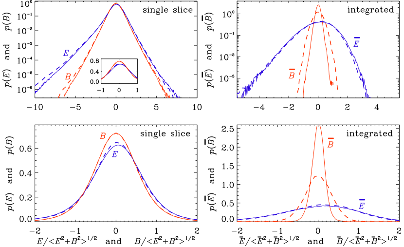
Figure 6.— Probability density functions of $E$ and $B$ polarization (left) and those of $\overline{E}$ and $\overline{B}$ (right) in semilogarithmic (top) and linear representations (bottom) for helical turbulence (the runs shown in Figures 4d–f of Brandenburg & Kahniashvili, 2017, solid lines) and nonhelical turbulence (Run A of Brandenburg et al., 2017, dashed lines).

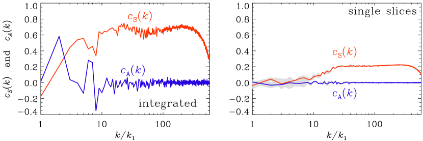
Figure 7.— Similar to Figure 5, but for dust polarization.

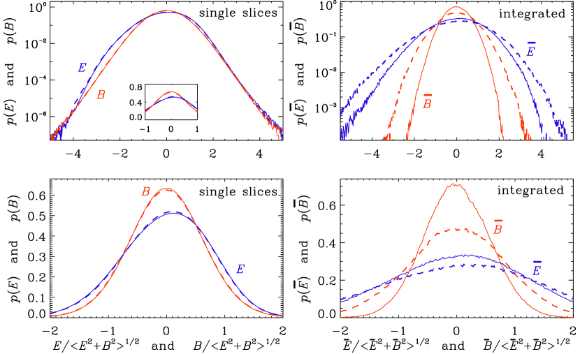
Figure 8.— Similar to Figure 6, but for dust polarization.

In Figure 5 we also see that $c_{\rm S}(k)$, based on the line-of-sight integral in Equation (2), approaches unity. In other words, the $EE$ polarization exceeds the $BB$ polarization by a factor of over a hundred in this case. This is surprising, because in each of the individual planes, e.g., that shown in Figure 4, the $EE$ correlation exceeds the $BB$ correlation only by a factor of about 2 at $k/k_{1}\approx 30$; see the second panel of Figure 5, which was also what was found by Kritsuk et al. (2018) using realistic simulations of supersonic turbulence. Here and elsewhere, error margins have been computed by using any one third of the original data and estimate the error as the largest departure from the full average.

To understand the reason for this, we must look for the possibility of excessive and preferential cancelation in $B(x,y)$ compared to $E(x,y)$. In this connection, we recall that, since the transformation from $(Q,U)$ to $(E,B)$ is a linear one, the line-of-sight integral in Equation (2) can also be carried out over $E+{\rm i}B$, which is what we do when we talk about preferential cancelation in $B$ compared to $E$.

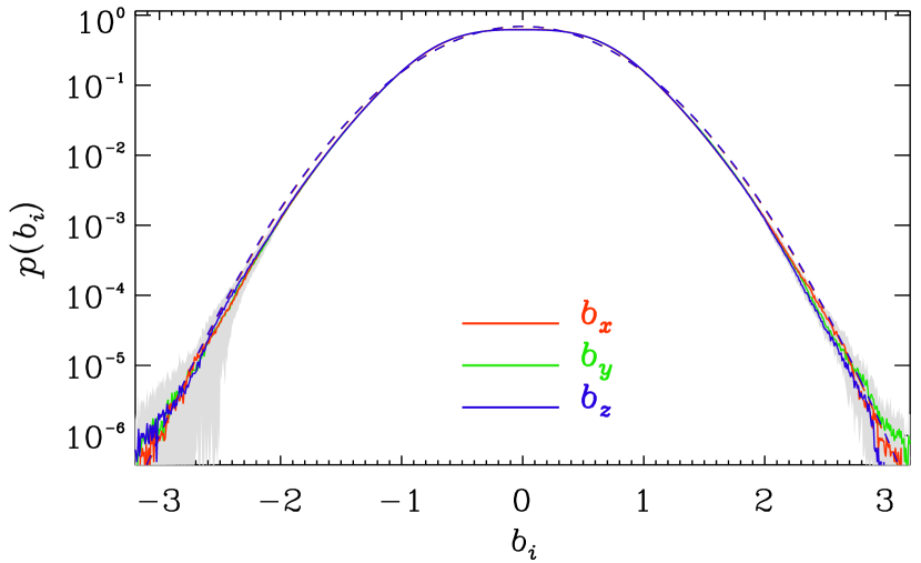
Figure 9.— Histogram of the three components of the magnetic field for the helical turbulence run.

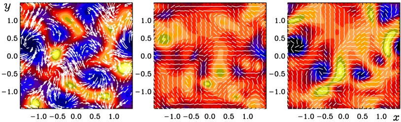
Figure 10.— Magnetic field vectors and line-of-sight component (color-coded; left) as well as $E$-mode (middle) and $B$-mode polarization (right) in rotating convection viewed from the top onto the convecting layer.

Table 1 Variance, skewness, and kurtosis for the distributions shown in Figure 6.

quantity helical? $E\;$ $B\;$ $\overline{E}\;$ $\overline{B}\;$ $\sigma$ yes $0.77$ $0.63$ $1.51$ $0.25$ no $0.77$ $0.64$ $1.65$ $0.58$ ${\rm skew}$ yes $-0.55$ $0.00$ $-0.45$ $-0.11$ no $-0.61$ $0.00$ $-0.53$ $-0.05$ ${\rm kurt}$ yes 3.09 1.54 0.56 0.58 no 3.87 1.69 0.84 0.08

Table 2 Similar to Table LABEL:Tskew, but for the case of dust emission shown in Figure 8.

quantity helical? $E\;$ $B\;$ $\overline{E}\;$ $\overline{B}\;$ $\sigma$ yes $0.76$ $0.65$ $1.21$ $0.56$ no $0.76$ $0.65$ $1.45$ $0.85$ ${\rm skew}$ yes $-0.19$ $0.00$ $-0.19$ $0.01$ no $-0.20$ $0.00$ $-0.24$ $-0.04$ ${\rm kurt}$ yes $-0.02$ $0.26$ $0.07$ $-0.04$ no $+0.03$ $0.24$ $0.16$ $0.00$

In Figure 6, we show the probability density functions of $E(x,y,z)$ and $B(x,y,z)$ and compare them with those of the line-of-sight or $z$-integrated values that we denote here by $\overline{E}(x,y)$ and $\overline{B}(x,y)$. Their variances are $\sigma_{E}^{2}=\langle E^{2}\rangle-\langle E\rangle^{2}$ and $\sigma_{B}^{2}=\langle B^{2}\rangle-\langle B\rangle^{2}$. In all cases, the averages are negligible, i.e., $\langle E\rangle^{2}\approx 0$ and $\langle B\rangle^{2}\approx 0$. It turns out that, while $B(x,y,z)$ and $\overline{B}(x,y)$ are symmetric about zero, $E(x,y,z)$ and $\overline{E}(x,y)$ are not. This is quantified by the skewness,

$${\rm skew}(E)=\langle E^{3}\rangle/\sigma_{E}^{3},\quad{\rm skew}(B)=\langle B^{3}\rangle/\sigma_{B}^{3}.$$ (14)

These values are listed in Table LABEL:Tskew both for helical and nonhelical turbulence. These simulations correspond to the runs shown in Figures 4d–f of Brandenburg & Kahniashvili (2017) for the helical case and Run A of Brandenburg et al. (2017) for the nonhelical case. For completeness, we also list there the kurtoses of those fields, which are defined as

$${\rm kurt}(E)=\langle E^{4}\rangle/\sigma_{E}^{4}-3,\quad{\rm kurt}(B)=\langle B^{4}\rangle/\sigma_{B}^{4}-3.$$ (15)

The consequences of a non-vanishing skewness of $E$ become clear when looking at the probability density functions of $\overline{E}(x,y)$ and $\overline{B}(x,y)$ in Figure 6, which show a dramatic difference for large values where $|E|>\sigma_{E}$, because now positive and negative pairs of equal strengths have different abundance or probability and do not cancel. The reason for this asymmetry lies in the nature of turbulence, which has a preference of producing large tails of negative $E$ polarization, which corresponds to a preference of radial over circular patterns.

In the results presented above, we have assumed that the local emissivity $\epsilon$ is proportional to $\bm{b}^{2}$, but this is not realistic in all astrophysical contexts as for instance in the case of dust polarization, which is the case for which an enhanced $EE/BB$ correlation ratio has been found. In Figure 7, we show that for constant $\epsilon$, i.e., independent of $|\bm{b}|$, we still find $c_{\rm S}>0$, but it is now no longer so close to unity as in the case when $\epsilon\propto\bm{b}^{2}$. Instead, we have $c_{\rm S}\approx 0.6$ for intermediate values of $k$, which corresponds to $C_{EE}/C_{BB}\approx 7$. The result for individual slices is, however, less strongly affected by the choice of $\epsilon$.

The corresponding probability density functions are shown in Figure 8. We see that the basic asymmetry of the probability density function of $E$ still persists both for individual slices and for the integrated maps, but the tails of the distribution are now less extended; see Table LABEL:Tskew_dust for the corresponding values of skewness and kurtosis. As already explained above, the asymmetry in $E$ results here from a dominance of circular patterns. However, even a preference of radial patterns would cause asymmetry, albeit with the other sign. Any such asymmetry would always lead to an excess of $EE$ correlations over $BB$ correlations and hence an enhanced $EE/BB$ ratio.

The relative importance of radial patterns over circular ones is a qualitatively new property of turbulent motions that needs to be studied further. It does not imply any asymmetry in the individual components of the magnetic field, as shown in Figure 9.

3.2. Convection

Next, we perform hydrodynamic simulations with gravity $\bm{g}=(0,0,-g)$ and angular velocity $\bm{\Omega}=(0,0,\Omega)$ in a layer $z_{\rm bot}\leq z\leq z_{\rm top}$, heated from below. Here $z_{\rm top}-z_{\rm bot}\equiv d$ is the thickness of the layer. The governing equations for density $\rho$, velocity $\bm{u}$, the specific entropy $S$, and the magnetic vector potential $\bm{a}$ are given by

$${{\rm D}{}\ln\rho\over{\rm D}{}t}=-{\bm{\nabla}}\cdot\bm{u},$$ (16)

$$\rho{{\rm D}{}\bm{u}\over{\rm D}{}t}=-{\bm{\nabla}}P+\rho\bm{g}-2\bm{\Omega}\times\rho\bm{u}+\bm{j}\times\bm{b}+{\bm{\nabla}}\cdot(2\nu\rho\mbox{\boldmath${\sf S}$}{}),$$ (17)

$$\rho T{{\rm D}{}S\over{\rm D}{}t}=K\nabla^{2}T+\eta\mu_{0}\bm{j}^{2}+2\nu\rho\mbox{\boldmath${\sf S}$}{}^{2},$$ (18)

$${\partial\bm{a}\over\partial t}=\bm{u}\times\bm{b}+\eta\nabla^{2}\bm{a},$$ (19)

where $P$ is the pressure with $S=c_{v}\ln P-c_{p}\ln\rho$, which is defined up to some additive constant, $c_{p}$ and $c_{v}$ are the specific heats at constant pressure and density, respectively, $T$ is the temperature with $P/\rho=(c_{p}-c_{v})T$ being the ideal gas equation of state, $K$ is the thermal diffusivity, $\nu$ is the kinematic viscosity, $\eta$ is the magnetic diffusivity, $\bm{b}=\bm{b}_{0}+{\bm{\nabla}}\times\bm{a}$ is the magnetic field with $\bm{b}_{0}$ being the imposed field, $\bm{j}={\bm{\nabla}}\times\bm{b}/\mu_{0}$ is the current density that was already defined in the introduction.

Table 3 Parameters for convection simulations.

Run Ra $\nu$ $\lambda$ $u_{\rm rms}$ Res. A 3600 0.01 0.35 0.050 $144^{2}\times 48$ B 14400 0.005 0.42 0.045 $288^{2}\times 96$

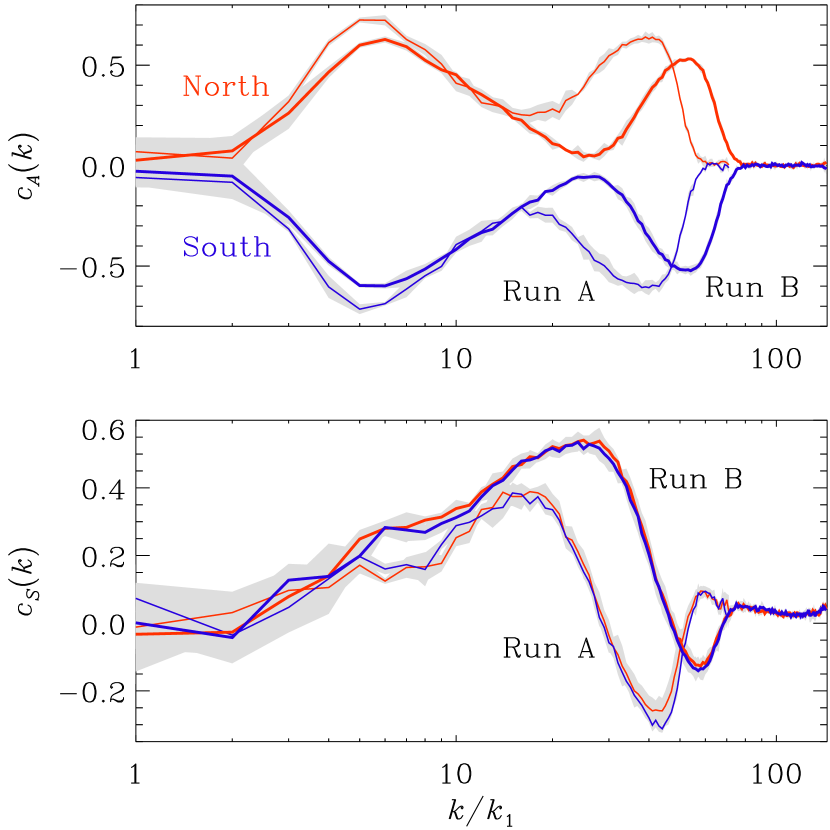
Figure 11.— $c_{\rm A}(k)$ (top) and $c_{\rm S}(k)$ (bottom) for convection simulations corresponding to the northern (red) and southern (blue) hemispheres for Runs A (thin lines) and B (thick lines). The gray shades indicate error bars obtained from the statistics over about 50 snapshots covering a time interval of about 1000 time units.

We adopt a polytropic stratification with background temperature $T=-gz/c_{\rm p}$, so $T=0$ at $z=0$. We fix $d$ and choose $|z_{\rm top}|/d$ to set the degree of stratification. The smaller $|z_{\rm top}|/d$, the stronger is the stratification, i.e., the stronger is the temperature contrast. In the following we choose $|z_{\rm top}|/d=0.1$, so the temperature changes by a factor of 10; see Hurlburt et al. (1984) for a similar setup. We choose $\bm{g}\cdot\bm{\Omega}$ to be either negative or positive, corresponding to the northern or southern hemispheres, respectively. A vertical magnetic field is imposed and tangled by this velocity field. The simulation setup is similar to that of Hurlburt & Toomre (1988), except that they did not include rotation, which makes our present simulations therefore closer to those of Brandenburg et al. (1990), which did include rotation.

In the following, we denote by $\rho_{0}$ the density at $z=-d$. Some of the parameters are listed in Table LABEL:Tconv. The imposed magnetic field points in the $z$ direction and is given by $B_{0z}=0.02B_{\rm eq}$, where $B_{\rm eq}^{2}=\mu_{0}\rho_{0}gd$ is the thermal equipartition field strength. We use $\Omega=0.2\,(g/d)^{1/2}$ in all cases. The Rayleigh number is defined as $(gd^{4}\rho_{\rm m}/\nu K)\,({\rm d}{}s/{\rm d}{}z)_{\rm m}$, where $\rho_{\rm m}$ and $({\rm d}{}s/{\rm d}{}z)_{\rm m}$ are density and the specific entropy of the hydrostatic solution in the middle of the domain.

Cross-sections of $\bm{b}(x,y)$, $E(x,y)$, and $B(x,y)$ near the surface are shown in Figure 10 for the results of such a simulation. One sees cyclonic convection in the northern hemisphere as viewed from the top, so all converging inflows attain a counterclockwise swirl, and all diverging outflows are clockwise swirl. A similar appearance is also attained by the magnetic field. It would be different when viewing this pattern from beneath that we would see as a mirror image of the original pattern and therefore the opposite sign of the $B$ polarization. The consequence of this can be seen in Figure 11, where we plot $c_{\rm S}(k)$ and $c_{\rm A}(k)$ for north (red) and south (blue) for Runs A and B whose parameters are summarized in Table LABEL:Tconv. There is now a systematic $EB$ correlation, so $c_{\rm A}(k)$ is positive in the north and negative in the south; Table LABEL:Tconvhel. This is very promising and agrees with our intuition.

Table 4 Result for convection, as shown in Figure 11.

Hemisph. $\bm{g}\cdot\bm{\Omega}$ $c_{\rm A}(k)$ $\langle\omega_{z}u_{z}\rangle$ $J_{z}B_{z}$ N $-$ $+$ $-$ $-$ S $+$ $-$ $+$ $+$

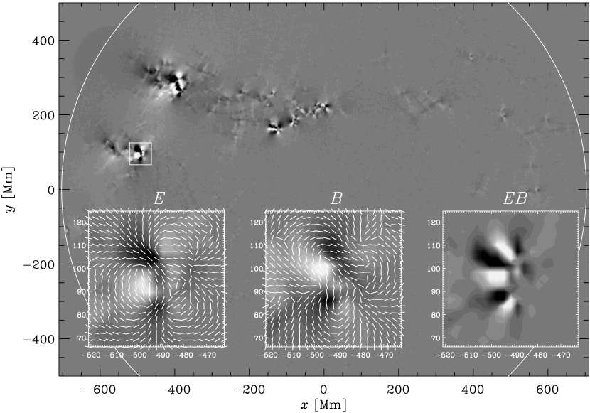
Figure 12.— Solar $E$, $B$, and $EB$ plots in the proximity of AR12325 on 2015–04–16 superimposed on the full disk image of $E$ polarization.

In rotating convection in the northern hemisphere, we have $\bm{g}\cdot\bm{\Omega}<0$. Near the upper surface, a downdraft ($u_{z}<0$) will suffer a counter-clockwise spin ($\omega_{z}>0$), so $\omega_{z}u_{z}<0$, corresponding to negative kinetic helicity. This applies to the sketch shown in Figure 1 (left, for downflows). Likewise, an updraft ($u_{z}>0$) will suffer a clockwise spin ($\omega_{z}<0$), so again $\omega_{z}u_{z}<0$, i.e., the kinetic helicity is unchanged and its sign equal to that of $\bm{g}\cdot\bm{\Omega}$. This applies to the sketch shown in Figure 1 (right, for upflows). Since the polarization vectors have no vector tip, both updrafts and downdrafts result in the same $E$ and $B$ polarization properties in each hemisphere. Therefore $EB$ is positive for $\bm{g}\cdot\bm{\Omega}<0$ (north) and negative for $\bm{g}\cdot\bm{\Omega}>0$ (south). In this case, $EB$ does reflect the sign of kinetic helicity, except that they are opposite to each other.

4. Prospects of finding solar $EB$ polarization

We now consider the Stokes $Q$ and $U$ parameters from the scattering emission on the solar surface. We ignore Stokes $I$ and $V$ and only look at $Q$ and $U$ at a fixed wavelength corresponding to the Fe I $630.15\,{\rm nm}$ line (see Hughes et al., 2016, for details of those data).

Figure 13.— $c_{\rm S}(k)$ and $c_{\rm A}(k)$ for the time average of all data from 2010 to 2017. For wavenumbers above $20\,{\rm Mm}^{-1}$, the data have been averaged over logarithmically spaced bins.

An example is shown in Figure 12 using data from the Synoptic Optical Long-term Investigations of the Sun (SOLIS) instrument of the NSO Integrated Synoptic Program (NISP). In the following, we analyze the full disk data such as the one shown in Figure 12. In the three insets, we show zoom-ins of $E$, $B$, and the product $EB$ to smaller patch whose location on the solar disk is indicated by a small square. In all cases, $E$ and $B$ are computed for the full disk, however.

The resolution of the full disk data is $2048^{2}$ pixels, but it turned out that the spectral power at the highest wavenumbers is rather small. Therefore, we downsampled the data to a resolution of $512^{2}$ points and we verified that no essential information is lost in this process.

To have a chance in finding a definite sign, we separate the signs in the northern and southern hemispheres by using the two-scale method discussed in Sect. 2.2. In Figure 13 we show the result for $c_{\rm S}(k)$ and $c_{\rm A}(k)$ for the years from 2010 to 2017. The statistical errors are generally large and there are strong sign changes for $k<0.03\,{\rm Mm}^{-1}$, suggesting that those values are uncertain. There is a short range of positive values of $c_{\rm A}(k)$ around $0.04\,{\rm Mm}^{-1}\mathrel{\mathchoice{\vbox{\offinterlineskip\halign{\hfil$\displaystyle#$\hfil\cr<\cr\sim\cr}}}{\vbox{\offinterlineskip\halign{\hfil$\textstyle#$\hfil\cr<\cr\sim\cr}}}{\vbox{\offinterlineskip\halign{\hfil$\scriptstyle#$\hfil\cr<\cr\sim\cr}}}{\vbox{\offinterlineskip\halign{\hfil$\scriptscriptstyle#$\hfil\cr<\cr\sim\cr}}}}k\mathrel{\mathchoice{\vbox{\offinterlineskip\halign{\hfil$\displaystyle#$\hfil\cr<\cr\sim\cr}}}{\vbox{\offinterlineskip\halign{\hfil$\textstyle#$\hfil\cr<\cr\sim\cr}}}{\vbox{\offinterlineskip\halign{\hfil$\scriptstyle#$\hfil\cr<\cr\sim\cr}}}{\vbox{\offinterlineskip\halign{\hfil$\scriptscriptstyle#$\hfil\cr<\cr\sim\cr}}}}0.1\,{\rm Mm}^{-1}$, but those values are still compatible with zero within error bars. This somewhat unexpected result remains subject to further investigations. As seen from Table LABEL:Tconvhel, positive values of $c_{\rm A}(k)$ correspond to negative magnetic helicity, which is expected for the northern hemisphere and compatible with our two-scale analysis, where the sign corresponds to that of the northern hemisphere. The wavenumber interval from $0.04$ to $0.1\,{\rm Mm}^{-1}$ agrees with that where most of the magnetic power has previously been found from the SOLIS data; see Singh et al. (2018). It might therefore be useful to target further work to this wavenumber range.

We also see that $c_{\rm S}(k)$ is fluctuating around zero. This shows that the $EE/BB$ correlation ratio is about unity, which is thus quite different from the Planck results for dust polarization. This suggests that the effect of line-of-sight integration discussed in Section 3.1 is here unimportant and could be a consequence of the optical thickness being large.

5. Conclusions

Our work has identified an important factor governing the enhanced ratio of $EE$ to $BB$ polarization: a strongly asymmetric $E$ distribution for helical (nonhelical) turbulence with a skewness of $-0.55$ ($-0.61$) and $-0.19$ ($-0.20$) for $\epsilon\propto\bm{b}^{2}$ and $\epsilon={\rm const}{}$, respectively, compared with an unskewed $B$ distribution. This implies that, depending on the extent of the line-of-sight integration, there will be less cancelation of $E$ compared to $B$, which explains the enhanced $EE$ to $BB$ ratio. This was previously explained in terms of Alfvén waves in magnetically dominated flows (Kandel et al., 2017).

Under inhomogeneous conditions, the $EB$ cross correlation is found to be a meaningful proxy of kinetic and magnetic helicity. We have shown that such conditions are found in stratified convection in the presence of rotation. This became clear from the sketch shown in Figure 1. Homogeneous systems, by contrast, are unable to produce any net $EB$ cross correlation, even if the turbulence is fully helical. This is because, with respect to a given line of sight, a helical eddy can face the observer at different viewing angles, where $B$ can attain positive and negative values, depending on which side of the plane the observer is facing, while the $E$ polarization can be similar in both cases, independently of the viewing angle. For convection, on the other hand, owing to inhomogeneity, it is impossible to find a local plane whose statistical $EB$ correlations agrees with one that is flipped, so there can be no cancelation. This was demonstrated by our numerical experiments, which show a dependence of the $EB$ correlation on the sign of $\bm{g}\cdot\bm{\Omega}$, and thus on the kinetic and magnetic helicities.

To assess the prospects of determining parity-odd polarization from solar scattering emission, we have employed the two-scale analysis to the oppositely helical contributions from north and south. Unfortunately, a clear antisymmetric spectral correlation could not be determined as yet. Even in the $k$ range between $0.04$ and $0.1\,{\rm Mm}^{-1}$, where most of the magnetic energy is known to reside in the SOLIS measurements (Singh et al., 2018), the positive values obtained for $c_{\rm A}(k)$ are compatible with zero. One reason for this poor hemispheric distinction could be that not all corrections applied to the final vector spectromagnetograph magnetic field data are included in the spectral data cubes for Stokes $I$, $Q$, $U$, and $V$ available from the SOLIS website. This issue needs to be investigated in future work.

$Header: /var/cvs/brandenb/tex/sayan/EBmodes/paper.tex,v 1.104 2018/11/21 17:34:59 brandenb Exp $

References

- Bai et al. (2014) Bai, X. Y., Deng, Y. Y., Teng, F., Su, J. T., Mao, X. J., & Wang, G. P. 2014, MNRAS, 445, 49
- Bourdin & Brandenburg (2018) Bourdin, Ph.-A., & Brandenburg, A. 2018, ApJ, in press, arXiv:1804.04160
- Bracco et al. (2018) Bracco, A., Candelaresi, S., Del Sordo, F., & Brandenburg, A. 2018, A&A, in press, arXiv:1807.10188
- Brandenburg (2001) Brandenburg, A. 2001, ApJ, 550, 824
- Brandenburg & Kahniashvili (2017) Brandenburg, A., & Kahniashvili, T. 2017, Phys. Rev. Lett., 118, 055102
- Brandenburg & Subramanian (2005) Brandenburg, A., & Subramanian, K. 2005, Phys. Rep., 417, 1
- Brandenburg et al. (2017) Brandenburg, A., Kahniashvili, T., Mandal, S., Roper Pol, A., Tevzadze, A. G., & Vachaspati, T. 2017, Phys. Rev. D, 96, 123528
- Brandenburg et al. (1990) Brandenburg, A., Nordlund, Å., Pulkkinen, P., Stein, R.F., & Tuominen, I. 1990, A&A, 232, 277
- Brandenburg et al. (2017) Brandenburg, A., Petrie, G. J. D., & Singh, N. K. 2017, ApJ, 836, 21
- Caldwell et al. (2017) Caldwell, R. R., Hirata, C., & Kamionkowski, M. 2017, ApJ, 839, 91
- Durrer (2008) Durrer, R. 2008, The Cosmic Microwave Background (Cambridge Catalogue, September 2008)
- Hughes et al. (2016) Hughes, A. L. H., Bertello, L., Marble, A. R., Oien, N. A., Petrie, G., & Pevtsov, A. A. 2016, arXiv:1605.03500
- Hurlburt et al. (1984) Hurlburt, N. E., Toomre, J., Massaguer, J. M. 1984, ApJ, 282, 557
- Hurlburt & Toomre (1988) Hurlburt, N. E., & Toomre, J. 1988, ApJ, 327, 920
- Kahniashvili et al. (2014) Kahniashvili, T., Maravin, Y., Lavrelashvili, G., & Kosowsky, A. 2014, Phys. Rev. D, 90, 083004
- Kamionkowski & Kosowsky (1999) Kamionkowski, M., & Kosowsky, A. 1999, Ann. Rev. Nucl. Part. Sci., 49, 77
- Kamionkowski et al. (1997a) Kamionkowski, M., Kosowsky, A., & Stebbins, A. 1997a, Phys. Rev. Lett., 78, 2058
- Kamionkowski et al. (1997b) Kamionkowski, M., Kosowsky, A., & Stebbins, A. 1997b, Phys. Rev. D, 55, 7368
- Kamionkowski & Kovetz (2016) Kamionkowski, M., & Kovetz, E. D. 2016, ARA&A, 54, 227
- Kandel et al. (2017) Kandel, D., Lazarian, A., & Pogosyan, D. 2017, MNRAS, 472, L10
- Kemel et al. (2011) Kemel, K., Brandenburg, A., & Ji, H. 2011, Phys. Rev. E, 84, 056407
- Krause & Rädler (1980) Krause, F., & Rädler, K.-H. 1980, Mean-field Magnetohydrodynamics and Dynamo Theory (Oxford: Pergamon Press)
- Kritsuk et al. (2018) Kritsuk, A. G., Flauger, R., & Ustyugov, S. D. 2018, Phys. Rev. Lett., 121, 021104
- Moffatt (1978) Moffatt, H. K. 1978, Magnetic Field Generation in Electrically Conducting Fluids (Cambridge: Cambridge Univ. Press)
- Park & Blackman (2012) Park, K., & Blackman, E. G. 2012, MNRAS, 423, 2120
- Pevtsov et al. (1995) Pevtsov, A. A., Canfield, R. C., & Metcalf, T. R. 1995, ApJ, 440, L109
- Planck Collaboration Int. XX (2015) Planck Collaboration Int. XX. 2015, A&A, 576, A105
- Planck Collaboration Int. XXX (2016) Planck Collaboration Int. XXX. 2016, A&A, 586, A133
- Planck Collaboration results XI (2018) Planck Collaboration results XI. 2018, A&A, DOI:10.1051/0004-6361/201832618, arXiv:1801.04945
- Roberts & Soward (1975) Roberts, P. H., & Soward, A. M. 1975, Astron. Nachr., 296, 49
- Seehafer (1990) Seehafer, N. 1990, Solar Phys., 125, 219
- Seljak & Zaldarriaga (1997) Seljak, U., & Zaldarriaga, M. 1997, Phys. Rev. Lett., 78, 2054
- Singh et al. (2018) Singh, N. K., Käpylä, M. J., Brandenburg, A., Käpylä, P. J., Lagg, A., & Virtanen, I. 2018, ApJ, 863, 182
- Skumanich & Lites (1987) Skumanich, A., & Lites, B. W. 1987, ApJ, 322, 473
- Zhang & Brandenburg (2018) Zhang, H., & Brandenburg, A. 2018, ApJ, 862, L17
- Zhang et al. (2014) Zhang, H., Brandenburg, A., & Sokoloff, D. D. 2014, ApJ, 784, L45
- Zhang et al. (2016) Zhang, H., Brandenburg, A., & Sokoloff, D. D. 2016, ApJ, 819, 146