Simplest Scoto-Seesaw Mechanism

Abstract

By combining the simplest (3,1) version of the seesaw mechanism containing a single heavy “right-handed” neutrino with the minimal scotogenic approach to dark matter, we propose a theory for neutrino oscillations. The “atmospheric” mass scale arises at tree level from the seesaw, while the “solar” oscillation scale emerges radiatively, through a loop involving the “dark sector” exchange. Such simple setup gives a clear interpretation of the neutrino oscillation lengths, has a viable WIMP dark matter candidate, and implies a lower bound on the neutrinoless double beta decay rate.

I Introduction

So far the only neutrino mass parameters which have been experimentally measured are the two mass square splittings associated with the “atmospheric” and “solar” neutrino oscillations McDonald:2016ixn ; Kajita:2016cak . Precision measurements at reactor and accelerator-based experiments An:2012eh ; Abe:2017uxa further strengthen the three-neutrino oscillation paradigm. The corresponding ratio of squared solar-to-atmospheric mass splittings is found to be deSalas:2017kay

$$\frac{\Delta m_{\rm SOL}^{2}}{\Delta m_{\rm ATM}^{2}}=0.0302_{-0.0010}^{+0.0012}$$ (1)

at 1 $\sigma$ C.L. This ratio is necessary in order to describe the neutrino oscillation data successfully. The existence of these two different mass scales could be indications that maybe the two mass scales arise from two very different mechanisms.

Likewise, despite our inability to pin down its nature, we have firm evidence for the existence of cosmological dark matter Bertone2005279 . Altogether, the lack of neutrino masses and of a viable dark matter candidate constitute two of the main drawbacks of the standard $\mathrm{SU(3)_{c}\otimes SU(2)_{L}\otimes U(1)_{Y}}$ model of particle physics whose minimal gauge structure we tacitly assume here.

Accommodating neutrino oscillation parameters within a minimal tree level type-I seesaw extension of the standard model requires two isosinglet fermion messengers  i.e. the (3,2) seesaw, instead of the “complete” sequential (3,3) seesaw scenario. Indeed, this (3,2) seesaw possibility, first suggested in Schechter:1980gr , has been recently studied in Ref. King:2015sfk . It is clear however that, in the presence of adequate radiative corrections, the minimal (3,1) type-I seesaw picture could be sufficient. Unfortunately, in such minimal (3,1) type-I seesaw setup the required mass splittings needed to describe solar neutrino oscillations do not emerge automatically. Moreover, the problem of having a suitable dark matter candidate remains unresolved. Here we show that both of these requirements can be met by consistently implementing the scotogenic mechanism proposed by Ernest Ma Ma:2006km .

In this letter we propose a scotogenic extension of the simplest (3,1) seesaw mechanism that provides a very clear interpretation of the two observed oscillation scales and the associated messengers. To first approximation we generate only the atmospheric scale, from the tree level exchange of the single isosinglet neutrino messenger present in the minimal (3,1) type-I seesaw mechanism Schechter:1980gr . At this stage two neutrinos are left massless, so there are no solar neutrino oscillations. We then show that this mass degeneracy is lifted by calculable radiative corrections of the scotogenic type. These involve the one-loop exchange of dark messengers, responsible for generating the solar scale, thus naturally accounting for the observed smallness of solar-to-atmospheric ratio in Eq. (1). The lightest radiative neutrino mass messenger associated to the solar mass scale provides the observed cosmological dark matter in the form of a thermal weakly interacting massive particle (WIMP).

II The minimal scotogenic seesaw

II.1 The Yukawa Sector

Here we describe our minimal scotogenic seesaw mechanism. Our basic template is the “incomplete” (3,1) type-I seesaw mechanism proposed in Ref. Schechter:1980gr , containing a single heavy isosinglet neutral lepton, we call $N$. To this we add a dark sector, odd under the assumed “dark $\mathbb{Z}_{2}$ parity”, consisting of one scalar $\eta$ and one fermion $f$, indicated in the last two columns of table 1. As mentioned, this theory is consistent, since gauge singlets carry no anomaly. The full Yukawa sector is given by:

$$\mathcal{L} = \mathcal{L_{\rm SM}}+\mathcal{L_{\rm ATM}}+\mathcal{L_{\rm DM,SOL}}$$ (2)

where $\mathcal{L_{\rm SM}}$ is the standard model Lagrangian and

$$\mathcal{L_{\rm ATM}} = -Y_{(N)}^{k}\overline{L}^{k}i\sigma_{2}H^{*}N\,+\,\frac{1}{2}M_{N}\overline{N^{c}}N\,+~{}h.c.$$ (3)

induces an effective non-zero tree level neutrino mass, once the electroweak symmetry is broken by the vacuum expectation value of the standard model Higgs. This scale is identified as the atmospheric scale.

	$N$	$\eta$	$f$
$\mathrm{SU(2)_{L}}$	1	2	1
$\mathrm{U(1)_{Y}}$	0	1/2	0
$\mathbb{Z}_{2}$	$+$	$-$	$-$
Multiplicity	1	1	1

Table 1: Messengers in the scotogenic extension of the minimal type-I seesaw model, called (3,1) in Schechter:1980gr .

Note that, by itself, Eq. (3) leads neither to a dark matter candidate, nor to solar neutrino oscillations. The minimal way to generate the solar neutrino mass scale is to add the two “dark” messenger fields, one boson and one fermion, indicated in the last two columns of table 1. Note that the fermion $f$ is intrinsically distinct from the isosinglet $N$ as it is odd under the $\mathbb{Z}_{2}$ symmetry. The Lagrangian responsible for the solar and dark sector is given by

$$\mathcal{L_{\rm DM,SOL}} = Y_{(f)}^{k}\overline{L}^{k}i\sigma_{2}\eta^{*}f\,+\frac{1}{2}M_{f}\overline{f^{c}}f+~{}h.c.$$ (4)

The quantum corrections coming from the “scotogenic” loop Ma:2006km will now induce the smaller solar scale.

Note that the last row in Table 1 indicates the minimum required field multiplicity ensuring the presence of one atmospheric seesaw messenger and the dark matter candidate, interpreted as the lighter of the messengers responsible for generating the solar neutrino scale.

In short, our proposal is the simplest scotogenic completion of the (3,1) seesaw model, defined in Eqs. (2,3,4). This minimal setup provides a very simple picture where the atmospheric scale arises at the tree level while the solar scale follows from calculable loop corrections, hence matching the observed smallness of one with respect to the other, given in Eq. (1). These features emerge Hirsch:2000ef ; diaz:2003as in more complicated supergravity schemes based upon spontaneous Masiero:1990uj or bilinear breaking of R parity Diaz:1997xc . However, within the supersymmetric picture, due to the breaking of R-parity, there is no stable WIMP dark matter candidate. In contrast, in the present much simpler setup, by construction the existence of WIMP dark matter is ensured.

II.2 The Scalar Sector

The scalar potential must include a second doublet $\eta$, with the same quantum numbers as the standard model Higgs doublet, but with $\mathbb{Z}_{2}$-odd parity. It can be written as

$$V = -m_{H}^{2}H^{\dagger}H+m_{\eta}^{2}\eta^{\dagger}\eta+\frac{1}{2}\lambda_{H}(H^{\dagger}H)^{2}+\frac{1}{2}\lambda_{\eta}(\eta^{\dagger}\eta)^{2}+\lambda_{3}(H^{\dagger}H)(\eta^{\dagger}\eta)+\lambda_{4}(H^{\dagger}\eta)(\eta^{\dagger}H)+\frac{1}{2}\lambda_{5}\Big{[}(H^{\dagger}\eta)^{2}+h.c.\Big{]}$$ (5)

Since the $\mathbb{Z}_{2}$ symmetry is exactly conserved, the mixings between the Higgs doublet and $\eta$ are forbidden. The mass spectrum for the components of the $\eta$ doublet are given by

$$m_{\eta^{R}}^{2} = m_{\eta}^{2}+\frac{1}{2}(\lambda_{3}+\lambda_{4}+\lambda_{5})v_{\phi}^{2}$$ (6)

$$m_{\eta^{I}}^{2} = m_{\eta}^{2}+\frac{1}{2}(\lambda_{3}+\lambda_{4}-\lambda_{5})v_{\phi}^{2}$$ (7)

$$m_{\eta^{+}}^{2} = m_{\eta}^{2}+\frac{1}{2}\lambda_{3}\,v_{\phi}^{2}~{}.$$ (8)

Note that the doublet $\eta$ in the scalar potential is analogous to the one present in the popular inert Higgs doublet model LopezHonorez:2006gr . However, in our present theory we have a new feature associated with the key role of the coupling $\lambda_{5}$, related to the breaking of lepton number responsible for solar neutrino mass generation Merle:2016scw , a feature absent in the inert Higgs doublet scheme .

III Neutrino Masses

III.1 Tree Level Structure

The tree level part of our model gives rise to a neutrino mass matrix $\mathcal{M}_{\nu}^{ij}$ given by

$$\mathcal{M}_{\nu}^{ij} = \left(\begin{array}[]{cccc}0&0&0&y^{1}_{(N)}v\\ 0&0&0&y^{2}_{(N)}v\\ 0&0&0&y^{3}_{(N)}v\\ y^{1}_{(N)}v&y^{2}_{(N)}v&y^{3}_{(N)}v&M_{N}\\ \end{array}\right)$$ (13)

in the basis $(L^{k},N)^{T}$. This clearly has a projective structure:

$$\mathcal{M}_{\nu~{}\rm TREE}^{ij} = -\frac{v^{2}}{M_{N}}Y_{(N)}^{i}Y_{(N)}^{j}$$ (14)

since the $N$ “pairs off” with only one combination of the neutrinos through the Dirac-like couplings. Here the indices $i,j=1,2,3$ are the flavour indices corresponding to the three generations of lepton doublets $L^{k}$. Choosing $M_{N}\,\sim\,10^{12}\,\text{GeV}$ (at the seesaw scale), $\mathbb{Y}_{(N)}\,\sim\,10^{-1}$, one reproduces the required value of the atmospheric scale.

III.2 Radiative Contributions

There are quantum corrections to Eq. (13) arising from loop diagrams. Most will simply correspond to renormalization of our (3,1) type-I seesaw mechanism, reproducing the same projective structure that leads to the masslessness of the two lighter neutrinos. These corrections are indicated by a blob in (21) given below,

$$\mathcal{M}_{\nu~{}\rm TOTAL}^{ij} = \left[\begin{array}[]{ccc}&&\\ &&\\ \quad\parbox{56.9055pt}{ \fmffile{radneutmassv2} \fmfgraph*(50,50) \fmfleft{i2,i1} \fmfright{o2,o1} \fmf{dashes}{i1,v1} \fmfdot{i1} \fmflabel{$\left<H\right>$}{i1} \fmf{dashes}{v1,o1} \fmfdot{o1} \fmflabel{$\left<H\right>$}{o1} \fmf{dashes,left=0.4,tension=0.4}{v2,v1} \fmf{dashes,left=0.4,tension=0.4}{v1,v4} \fmf{plain_arrow,label=$\nu$,l.s=left}{i2,v2} \fmf{plain_arrow,tension=0.4}{v2,v3} \fmf{plain_arrow,tension=0.4}{v4,v3} \fmf{plain_arrow,label=$\nu$,l.s=right}{o2,v4} }&&\quad\quad\parbox{56.9055pt}{ \fmffile{nnmat24} \fmfgraph*(50,50) \fmfleft{i1,i2} \fmfright{o1} \fmf{plain_arrow}{v1,i1} \fmflabel{$N$}{i1} \fmf{dashes}{i2,v1} \fmflabel{$\left<H\right>$}{i2} \fmfblob{.2w}{v1} \fmf{plain_arrow}{o1,v1} \fmflabel{$\nu$}{o1} \fmfdot{i2} }\vskip 12.0pt plus 4.0pt minus 4.0pt\quad\quad\quad\\ &&\\ &&\\ \vskip 12.0pt plus 4.0pt minus 4.0pt\quad\quad\quad\quad\parbox{56.9055pt}{ \fmffile{nnmat20} \fmfgraph*(50,50) \fmfleft{i1,i2} \fmfright{o1} \fmf{plain_arrow}{i1,v1} \fmflabel{$\nu$}{i1} \fmf{dashes}{i2,v1} \fmflabel{$\left<H\right>$}{i2} \fmfblob{.2w}{v1} \fmf{plain_arrow}{v1,o1} \fmflabel{$N$}{o1} \fmfdot{i2} }\vskip 12.0pt plus 4.0pt minus 4.0pt\quad\quad&&\quad\quad\parbox{56.9055pt}{ \fmffile{nnmat26} \fmfgraph*(50,50) \fmfleft{i1} \fmfright{o1} \fmf{plain_arrow}{i1,v1} \fmflabel{$N$}{i1} \fmfblob{.2w}{v1} \fmf{plain_arrow}{o1,v1} \fmflabel{$N$}{o1} }\quad\end{array}\right]$$ (21)

Such corrections only redefine the parameters and do not add a new independent neutrino mass scale, needed in order to account for solar neutrino oscillations. Hence the mechanism generating the latter must be intrinsically different from the N-mediated seesaw. In order to implement this we clone our (3,1) seesaw mechanism with an independent low-scale mechanism of neutrino mass generation Boucenna:2014zba ; Cai:2017jrq of the scotogenic type Ma:2006km ; Ma:2008cu ; Hirsch:2013ola ; Hernandez:2013dta ; Aranda:2015xoa ; Ding:2016wbd ; Borah:2016zbd ; Wang:2017mcy . This last step is crucial in order to complete the theory with an experimentally testable dark matter sector.

radneutmass (70,70) i2,i1 o2,o1 dashesi1,v1 i1 $\left<H\right>$i1 dashesv1,o1 o1 $\left<H\right>$o1 dashes,label=$\eta_{R}$ ($\eta_{I}$),left=0.4,tension=0.4v2,v1 dashes,label=$\eta_{R}$ ($\eta_{I}$),left=0.4,tension=0.4v1,v4 plain_arrow,label=$L$,l.s=lefti2,v2 plain_arrow,tension=0.4v2,v3 $f$v3 plain_arrow,tension=0.4v4,v3 plain_arrow,label=$L$,l.s=righto2,v4

Figure 1: Radiative neutrino mass involving dark sector exchange, leading to a calculable solar neutrino mass scale.

In this case there are genuinely calculable quantum corrections arising from Fig. (1), and involving the exchange of the scalar and fermionic dark messengers $\eta$ and $f$. Though also projective, these corrections can not be renormalized away, and break the degeneracy of neutrino masses intrinsic to the “incomplete” nature of the (3,1) type-I template seesaw mechanism. The total neutrino mass has the structure

$$\mathcal{M}_{\nu~{}\rm TOT}^{ij} = -\frac{v^{2}}{M_{N}}Y_{(N)}^{i}Y_{(N)}^{j}\,+\,\mathcal{F}\left(m_{\eta^{R}},m_{\eta^{I}},M_{f}\right)M_{f}Y_{(f)}^{i}Y_{(f)}^{j}$$ (22)

where the function $\mathcal{F}$ is a loop function, expressed as the difference of two $B_{0}$-Veltman functions, namely,

$$\mathcal{F}\left(m_{\eta^{R}},m_{\eta^{I}},M_{f}\right) = \frac{1}{32\pi^{2}}\left[\frac{m_{\eta^{R}}^{2}\log\left({M_{f}^{2}/m_{\eta^{R}}^{2}}\right)}{M_{f}^{2}-m_{\eta^{R}}^{2}}-\frac{m_{\eta^{I}}^{2}\log\left({M_{f}^{2}/m_{\eta^{I}}^{2}}\right)}{M_{f}^{2}-m_{\eta^{I}}^{2}}\right]$$ (23)

One sees that these are “genuine” corrections with a different structure, that can lift the degeneracy and thus generate the solar neutrino mass splitting. Moreover, these are parametrically unrelated to the tree level masses. As shown above in (21), it is simple to understand in diagrammatic form the different structure of the tree and loop contributions. Moreover, given the projective nature of both terms in Eq. (22) one of the three neutrinos remains massless.

We now give a simple estimate of the relevant parameters required in order to account for the observed neutrino oscillations. The solar and the atmospheric square mass differences can be estimated by each of the eigenvalues of the tree level and radiative contributions to the neutrino mass matrix in Eq. (22)

$$\Delta m_{\rm ATM}^{2} \sim \left(\frac{v^{2}}{M_{N}}\mathbb{Y}_{(N)}^{2}\right)^{2}\,,\quad\Delta m_{\rm SOL}^{2}\,\sim\,\left(\frac{1}{32\pi^{2}}\right)^{2}\left(\frac{\lambda_{5}v^{2}}{M_{f}^{2}-m_{\eta}^{(R)2}}M_{f}\mathbb{Y}_{(f)}^{2}\right)^{2}.$$ (24)

The expression for $\Delta m_{\rm SOL}^{2}$ is obtained through Eqs. (6) and (7), where we take $M_{f}^{2},\,m_{\eta}^{(R)2},\,M_{f}^{2}-m_{\eta}^{(R)2}\gg\lambda_{5}v^{2}$, defining $\mathbb{Y}_{(a)}^{2}=\left(Y_{(a)}^{e}\right)^{2}\,+\,\left(Y_{(a)}^{\mu}\right)^{2}\,+\,\left(Y_{(a)}^{\tau}\right)^{2}$ for $a=f,N$, which summarizes the role of the Yukawa couplings.

Hence, the ratio between the solar and atmospheric square mass differences can be estimated by:

$$\frac{\Delta m_{\rm SOL}^{2}}{\Delta m_{\rm ATM}^{2}} \sim \left(\frac{1}{32\pi^{2}}\right)^{2}\lambda_{5}^{2}\left(\frac{M_{N}M_{f}}{M_{f}^{2}-m_{\eta}^{(R)2}}\right)^{2}\left(\frac{\mathbb{Y}_{(f)}^{2}}{\mathbb{Y}_{(N)}^{2}}\right)^{2}$$ (25)

A priori, the mass of the right handed neutrino $M_{N}$ and that of the dark sector fermion $M_{f}$ are two independent parameters that, in principle, can have very different values. As an example, the case of scalar WIMP dark matter can be realized by choosing $M_{N}\,\sim\,10^{12}\,\text{GeV}$, $M_{f}\sim 10^{4}\,\text{GeV}$, $m_{\eta}^{(R)}\,\sim\,10^{3}\,\text{GeV}$, $\mathbb{Y}_{(N)}\,\sim\,10^{-1}$, $\mathbb{Y}_{(f)}\sim 10^{-4}$, it can easily fit the solar and atmospheric scales as well as their ratio in Eq. (1), as long as one takes an adequately small value for $\lambda_{5}$. The latter indicates symmetry protection since, as $\lambda_{5}\to 0$, lepton number is recovered in the radiative sector. However, the masses of $N$ and $f$ can be quite similar to each other. For example, keeping other parameters as before one can also have $M_{N}\approx M_{f}\approx 10^{4}$ GeV for $\mathbb{Y}_{(N)}\,\sim\,10^{-5}$ and $\mathbb{Y}_{(f)}\sim 10^{-4}$. An alternative benchmark with intermediate mass values $M_{N}\approx M_{f}\approx 10^{6}$ GeV is obtained for $\mathbb{Y}_{(N)}\,\sim\,10^{-4}$ and $\mathbb{Y}_{(f)}\sim 10^{-3}$. Clearly, many other choices for masses and couplings can be found using Eq. (25). The upshot of the discussion is that one can easily fit Eq. (1), by making reasonable parameter choices.

IV Lepton Flavour Violation

Before closing, let us comment briefly on lepton flavour violation. Our model contains sources of lepton flavour violation, arising from the new Yukawa couplings $Y_{f}$ and $Y_{N}$ associated to the “scotogenic” and “seesaw” sectors of the theory. These lead to processes such as $\mu\to e\gamma$, $\mu\to 3e$ and muon-to-electron conversion in nuclei. For adequate $M_{N}$ and $Y_{N}$ values able to reproduce the required value of the neutrino mass scales in Eq. 24, the “scotogenic” contribution is by far the dominant one, hence we neglect the others . The lepton flavour violating branching fractions for $\mu\to e\gamma$ and $\mu\to 3e$ are given as

$$BR\left(\mu\to e\gamma\right) \approx \frac{\alpha m_{\mu}}{\left(8\pi\right)^{4}\Gamma_{t}}\left(\frac{m_{\mu}}{m_{\eta}}\right)^{4}\left(Y_{f}^{1}Y_{f}^{2}\right)^{2}\,\left(F\left(\frac{M_{f}^{2}}{m_{\eta}^{2}}\right)\right)^{2}$$ (26)

$$BR\left(\mu\to 3e\right) \approx \frac{\alpha^{2}m_{\mu}}{\left(8\pi\right)^{5}\Gamma_{t}}\left(\frac{m_{\mu}}{m_{\eta}}\right)^{4}\left(Y_{f}^{1}Y_{f}^{2}\right)^{2}\,G\left(\frac{m_{\mu}}{m_{e}}\right)\left(F\left(\frac{M_{f}^{2}}{m_{\eta}^{2}}\right)\right)^{2}$$ (27)

In these expressions $\Gamma_{t}$ is the total muon decay width, which is approximately $3\cdot 10^{-19}\,\text{GeV}$, while the functions $F$ and $G$ have the form

$$F(x) = \frac{2\,-\,9x\,+\,18x^{2}\,-\,11x^{3}\,+\,6x^{3}\log\left(x\right)}{6\left(1\,-\,x\right)^{4}}$$ (28)

$$G(x) = \frac{16}{3}\log\left(x\right)\,-\,\frac{22}{3}$$ (29)

Notice the presence of the $\alpha$ factor in addition to the phase space suppression in the $\mu\to 3e$ decay. Owing to this suppression the most stringent constraints on our model will come from the $\mu\to e\gamma$ decay.

For illustration, we show in Fig. 2 the results for the $\mu\to e\gamma$ branching ratio in our model. The contours have a fixed value of the branching fraction, as indicated on the right.

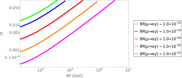
Figure 2: Isocontour plots for $BR\left(\mu\to e\gamma\right)$ in the $M_{f}$ vs $Y_{f}$ plane.

One can see that the expected values for the lepton flavour violating branching fractions for the benchmarks used in sec. III.2 fall well within the experimental upper bounds for $BR\left(\mu\to e\gamma\right)\sim 4.2\cdot 10^{-13}$ and $BR\left(\mu\to 3e\right)\sim 1.0\cdot 10^{-12}$ Tanabashi:2018oca . A dedicated study of lepton flavour violation within our model is outside the scope of this paper, and related material for the scotogenic model can be found in Refs. Toma:2013zsa ; Vicente:2014wga .

V Discussion and outlook

Having proposed the minimal setup for neutrino mass and dark matter, some comments are in order. First we note that neutrino masses arise from the interplay of tree level and quantum corrections, in a way reminiscent of supersymmetric models with bilinear breaking of R-parity. However, our theory is much simpler and, by construction, more complete, as it naturally incorporates the existence of a dark matter particle. The setup is minimalistic, though realistic, having effectively two messengers, the tree-level seesaw atmospheric messenger, and the radiative dark messenger responsible for inducing solar neutrino oscillations. Given the fact that one of the three neutrinos is massless in our model, and given the current information on the neutrino oscillation parameters deSalas:2017kay , one finds that the neutrinoless double beta decay ($\rm 0\nu\beta\beta$) amplitude never vanishes Reig:2018ztc . Indeed, the “incomplete messenger” structure of our model translates into a lower bound for $\rm 0\nu\beta\beta$. This holds even if the ordering of light neutrino mass eigenvalues is of the normal type, as currently preferred by the oscillation data.

Concerning dark matter we stress that the model has a built-in dark matter candidate that can be detected by nuclear recoil experiments such as Xenon-1T Aprile:2018dbl ; Aprile:2017iyp . Alternative options as well as extended scenarios can, however, easily be envisaged. In fact, possible variations of the original scotogenic model suggest new realizations of the idea proposed here. New charged fermions odd under the $\mathbb{Z}_{2}$ symmetry can be added instead of, or in addition to, the neutral fermion $f$ in table 1. For example, one can replace the fermion $f$ by a hyperchargeless isotriplet $\Sigma$, as in Ma:2008cu or add this triplet field altogether, as in Hirsch:2013ola . The dark matter candidate could then be an isotriplet-isosinglet fermion mixture or a scalar boson, generating new radiative contributions to the effective neutrino mass matrix in Eq. (22). There will be a wider parameter space for obtaining the correct relic density Hirsch:2013ola , as well as a consistent high energy behavior of the required $\mathbb{Z}_{2}$ symmetry Merle:2016scw . Likewise, a rich pattern of lepton flavour violating processes, such as $\mu\to e+\gamma$, $\mu\to 3e$ and $\mu-e$ conversion in nuclei is expected, as well as new possibilities concerning the issue of leptogenesis. In short, despite its simplicity and minimality, the model exhibits a rich phenomenological potential which deserves dedicated study. We intend to explore them in a future work.

VI Summary

We have proposed the simplest scotogenic extension of the minimum type-I seesaw scenario as a way to explain the hierarchy observed between the solar and atmospheric neutrino mass scales, Eq. (1), as well as to harbor a viable dark matter candidate. The template is the (3,1) type-I seesaw mechanism proposed in Schechter:1980gr characterized by an “incomplete” lepton sector consisting of a single “right-handed” neutrino. The setup is the minimal way to generate neutrino masses consistently, as well as the WIMP dark matter candidate. It gives a clear interpretation of the solar and atmospheric oscillation scales and the associated messengers. In the tree-level approximation one generates only the atmospheric scale, from the exchange of the single right-handed neutrino present in the (3,1) type-I seesaw mechanism, while the solar scale arises from calculable loop corrections mediated by the dark sector.

- (1) A. B. McDonald, “Nobel Lecture: The Sudbury Neutrino Observatory: Observation of flavor change for solar neutrinos,” Rev. Mod. Phys. 88 no. 3, (2016) 030502.
- (2) T. Kajita, “Nobel Lecture: Discovery of atmospheric neutrino oscillations,” Rev. Mod. Phys. 88 no. 3, (2016) 030501.
- (3) DAYA-BAY Collaboration Collaboration, F. An et al., “Observation of electron-antineutrino disappearance at Daya Bay,” Phys.Rev.Lett. 108 171803, arXiv:1203.1669 [hep-ex].
- (4) T2K Collaboration, K. Abe et al., “Combined Analysis of Neutrino and Antineutrino Oscillations at T2K,” Phys. Rev. Lett. 118 no. 15, (2017) 151801, arXiv:1701.00432 [hep-ex].
- (5) P. F. de Salas et al., “Status of neutrino oscillations 2018: 3 hint for normal mass ordering and improved CP sensitivity,” Phys. Lett. B782 (2018) 633–640, arXiv:1708.01186 [hep-ph]. http://globalfit.astroparticles.es/.
- (6) G. Bertone, D. Hooper, and J. Silk, “Particle dark matter: evidence, candidates and constraints,” Physics Reports 405 no. 5–6, 279–390. .
- (7) J. Schechter and J. W. F. Valle, “Neutrino Masses in SU(2) x U(1) Theories,” Phys. Rev. D22 (1980) 2227.
- (8) S. F. King, “Neutrino Mass and Mixing in the Seesaw Playground,” Nucl. Phys. B908 (2016) 456–466, arXiv:1511.03831 [hep-ph].
- (9) E. Ma, “Verifiable radiative seesaw mechanism of neutrino mass and dark matter,” Phys.Rev. D73 077301, arXiv:hep-ph/0601225 [hep-ph].
- (10) M. Hirsch, M. A. Diaz, W. Porod, J. C. Romao, and J. W. F. Valle, “Neutrino masses and mixings from supersymmetry with bilinear R parity violation: A Theory for solar and atmospheric neutrino oscillations,” Phys. Rev. D62 (2000) 113008, arXiv:hep-ph/0004115 [hep-ph]. [Erratum: Phys. Rev.D65,119901(2002)].
- (11) M. A. Diaz et al., “Solar neutrino masses and mixing from bilinear R-parity broken supersymmetry: Analytical versus numerical results,” Phys. Rev. D68 013009, hep-ph/0302021.
- (12) A. Masiero and J. W. F. Valle, “A Model for Spontaneous R Parity Breaking,” Phys.Lett. B251 (1990) 273–278.
- (13) M. A. Diaz, J. C. Romao, and J. W. F. Valle, “Minimal supergravity with R-parity breaking,” Nucl.Phys. B524 (1998) 23–40, arXiv:hep-ph/9706315 [hep-ph].
- (14) L. Lopez Honorez, E. Nezri, J. F. Oliver, and M. H. Tytgat, “The Inert Doublet Model: An Archetype for Dark Matter,” JCAP 0702 028, arXiv:hep-ph/0612275 [hep-ph].
- (15) A. Merle, M. Platscher, N. Rojas, J. W. F. Valle, and A. Vicente, “Consistency of WIMP Dark Matter as radiative neutrino mass messenger,” JHEP 07 (2016) 013, arXiv:1603.05685 [hep-ph].
- (16) S. M. Boucenna, S. Morisi, and J. W. F. Valle, “The low-scale approach to neutrino masses,” Adv. High Energy Phys. 2014 (2014) 831598, arXiv:1404.3751 [hep-ph].
- (17) Y. Cai, J. Herrero-García, M. A. Schmidt, A. Vicente, and R. R. Volkas, “From the trees to the forest: a review of radiative neutrino mass models,” arXiv:1706.08524 [hep-ph].
- (18) E. Ma and D. Suematsu, “Fermion Triplet Dark Matter and Radiative Neutrino Mass,” Mod.Phys.Lett. A24 583–589, arXiv:0809.0942 [hep-ph].
- (19) M. Hirsch, R. Lineros, S. Morisi, J. Palacio, N. Rojas, et al., “WIMP dark matter as radiative neutrino mass messenger,” JHEP 1310 149, arXiv:1307.8134 [hep-ph].
- (20) A. E. Carcamo Hernandez, I. de Medeiros Varzielas, S. G. Kovalenko, H. Pas, and I. Schmidt, “Lepton masses and mixings in an multi-Higgs model with a radiative seesaw mechanism,” Phys. Rev. D88 no. 7, (2013) 076014, arXiv:1307.6499 [hep-ph].
- (21) A. Aranda and E. Peinado, “A new radiative neutrino mass generation mechanism with higher dimensional scalar representations and custodial symmetry,” Phys. Lett. B754 (2016) 11–13, arXiv:1508.01200 [hep-ph].
- (22) R. Ding, Z.-L. Han, Y. Liao, and W.-P. Xie, “Radiative neutrino mass with dark matter: from relic density to LHC signatures,” JHEP 05 (2016) 030, arXiv:1601.06355 [hep-ph].
- (23) D. Borah and A. Dasgupta, “Common Origin of Neutrino Mass, Dark Matter and Dirac Leptogenesis,” JCAP 1612 no. 12, 034, arXiv:1608.03872 [hep-ph].
- (24) W. Wang, R. Wang, Z.-L. Han, and J.-Z. Han, “The Scotogenic Models for Dirac Neutrino Masses,” arXiv:1705.00414 [hep-ph].
- (25) Particle Data Group Collaboration, M. Tanabashi et al., “Review of Particle Physics,” Phys. Rev. D98 no. 3, (2018) 030001.
- (26) T. Toma and A. Vicente, “Lepton Flavor Violation in the Scotogenic Model,” JHEP 01 (2014) 160, arXiv:1312.2840 [hep-ph].
- (27) A. Vicente and C. E. Yaguna, “Probing the scotogenic model with lepton flavor violating processes,” JHEP 02 (2015) 144, arXiv:1412.2545 [hep-ph].
- (28) M. Reig, D. Restrepo, J. W. F. Valle, and O. Zapata, “Bound-state dark matter with Majorana neutrinos,” arXiv:1806.09977 [hep-ph].
- (29) XENON Collaboration, E. Aprile et al., “Dark Matter Search Results from a One TonneYear Exposure of XENON1T,” arXiv:1805.12562 [astro-ph.CO].
- (30) XENON Collaboration, E. Aprile et al., “First Dark Matter Search Results from the XENON1T Experiment,” Phys. Rev. Lett. 119 no. 18, (2017) 181301, arXiv:1705.06655 [astro-ph.CO].