Guidesort: Simpler Optimal Deterministic Sorting for the Parallel Disk Model

Abstract

A new algorithm, Guidesort, for sorting in the uniprocessor variant of the parallel disk model (PDM) of Vitter and Shriver is presented. The algorithm is deterministic and executes a number of (parallel) I/O operations that comes within a constant factor $C$ of the optimum. The algorithm and its analysis are simpler than those proposed in previous work, and the achievable constant factor $C$ of essentially 3 appears to be smaller than for all other known deterministic algorithms, at least for plausible parameter values.

Keywords: Parallel sorting, parallel disk model, PDM, external memory, Guidesort.

1 Introduction

Sorting is an important problem. In the seventies Knuth quoted an estimate that over 25% of computers’ running time is spent on sorting [7]. Frequently the data sets to be sorted are so large that they do not fit in internal memory and must be held on external storage, often one or more magnetic disks or similar devices. In this setting of massive data, sorting acquires even more importance because a high number of algorithms that use external storage efficiently do so by reducing other problems to sorting, so that the time to sort can almost be viewed as playing the role that linear time has in RAM computation.

Accesses to magnetic disks are much slower than CPU operations and accesses to internal memory. A natural and increasingly popular way to sort faster is to use many disks in parallel. Magnetic disks have high latencies, so efficiency dictates that an access to a magnetic disk must be used to transfer not one data item, but a whole block of many data items. The parallel disk model of Vitter and Shriver [14] tries to capture these characteristics of disk systems and has been used for much of the extensive research on sorting with several disks.

1.1 Model and Problem Statement

An instance of the uniprocessor variant of the parallel disk model or PDM of Vitter and Shriver [14] is specified via three positive integers, $M$, $B$ and $D$ with $2B\leq M$. It features a machine comprising an internal memory of $M$ cells and $D$ disks, each with an infinite number of cells. Every disk is linearly ordered and partitioned into block frames of $B$ consecutive cells, each of which can accommodate a block of $B$ data items. In slight deviation from the original definition of the PDM, we will assume that the internal memory is also linearly ordered and partitioned into block frames of $B$ consecutive cells and—therefore—that $M/B$ is an integer. An I/O operation or, for short, an I/O can copy the blocks stored in $D$ pairwise distinct block frames in the internal memory to block frames on $D$ pairwise distinct disks (an output operation) or vice versa (an input operation). Thus the disks are assumed to be synchronized. The description in [14] does not indicate explicitly whether it is also possible to transfer fewer than $D$ blocks between pairwise distinct block frames in the internal memory and block frames on as many pairwise distinct disks; here we will assume this to be the case. Arbitrary computation (internal computation) can take place on data stored in the internal memory, whereas items stored on disks can participate in computation only after being input to the internal memory. An algorithm is judged primarily by the number of I/O operations that it executes, computation in the internal memory usually being considered free.

So that operations in the internal memory and I/O operations can specify their arguments, we assume that the disks, the cells in the internal memory and the block frames both in the internal memory and on each disk are numbered consecutively, starting at 0 (say). A number of conventions make the PDM convenient to argue about, but less precise. First, the meaning of a “cell” depends on the problem under consideration. In the context of sorting, as relevant here, a cell is the amount of memory needed to store one of the items to be sorted or a comparable object (e.g., for sorting it is generally assumed that one can ensure at no cost that the keys of the input items are pairwise distinct by appending to each its position in the input). Second, the only space accounted for is that taken up by “data items”, not that needed to realize the control structure of an algorithm under execution. E.g., algorithms like those discussed in the following may want to manipulate such data structures as a recursion stack and various vectors indexed by disk numbers. Space for such bookkeeping information is assumed implicitly to be available whenever needed.

It is customary to restrict the parallel disk model by imposing an additional condition that says, informally, that $M$ is sufficiently large relative to $B$ and $D$. The condition varies from description to description, however, and seems to reflect the requirements of particular algorithms more than any fundamental deliberation concerning the model. E.g., [14] requires that $D\leq\Tfloor{{M/B}}$, [3] that $M\geq 2DB$, and [11] that $DB\leq\Tfloor{{{(M-M^{\beta})}/2}}$ for some fixed $\beta<1$. Since no more than $M/B$ disks can take part in a (parallel) I/O operation, the condition $D\leq{M/B}$ seems somewhat more canonical than the others, and we will adopt it here (alternatively, $D$ can be interpreted as the minimum of $M/B$ and a true number of disks). It cannot be a priori excluded, however, that more than $M/B$ disks can be put to good use in a PDM algorithm (cf. the RAMBO model of Fredman and Saks [5]).

A sequence of items is said to be stored in the striped format if its blocks are distributed over the disks in a round-robin fashion. More precisely, a sequence $(x_{0},\ldots,x_{N-1})$ is stored in the striped format if there are (known) nonnegative integers $a_{0},\ldots,a_{D-1}$ such that the following holds for $i=0,\ldots,N-1$: If $\Tfloor{{i/B}}=qD+r$ for integers $q$ and $r$ with $q\geq 0$ and $0\leq r<D$, then $x_{i}$ is the item numbered $i\bmod B$ in the block frame numbered $a_{r}+q$ on the disk numbered $r$. Every sequence for which nothing else is stated explicitly in the following is assumed to be stored in the striped format.

The problem of sorting in the PDM is defined as follows: Given as input a sequence $(x_{0},\ldots,x_{N-1})$, stored in the striped format, of items with a partial order defined by keys drawn from a totally ordered universe, output a sequence of the form $(x_{\sigma(0)},\ldots,x_{\sigma(N-1)})$, again stored in the striped format, where $\sigma$ is a bijection from $\{0,\ldots,N-1\}$ to $\{0,\ldots,N-1\}$ with $x_{\sigma(0)}\leq\cdots\leq x_{\sigma(N-1)}$.

1.2 The Challenge

In the remainder of the paper, consider the problem of sorting a sequence of $N>M$ items and take $n=\Tceil{N/B}$ (the number of block frames occupied by the input) and $m={M/B}$ (the number of block frames in the internal memory). Without loss of generality we will assume that the $N$ items to be sorted have pairwise distinct keys. The last of the $n$ blocks of input may contain a segment of data beyond the $N$ items to be sorted. Such a “foreign” segment should be treated as a sorted sequence of dummy items larger than all real items, so that the segment will not be modified by the sorting.

In the sequential case, i.e., for $D=1$, we can sort within $\Tvn{Sort}_{M,B}(N)=2n(1+\Tceil{\log_{m}({N/M})})=2n\Tceil{\log_{m}\!n}$ I/Os by first forming $\Tceil{N/M}$ sorted runs of at most $M$ items each and then merging the runs in an $m$-ary tree of height $\Tceil{\log_{m}({N/M})}$ (a more practical algorithm uses $(m-1)$-way merging instead of $m$-way merging at a slight loss of theoretical efficiency). A method for obtaining a nearly matching lower bound of ${{\Tvn{Sort}_{M,B}(N)}/(1+F(M,B,N))}$, where

$$F(M,B,N)=O\left(\frac{1}{\ln m}+\frac{1}{\log_{m}\!n}+\frac{\log_{m}\!n}{B}\right),$$

was indicated in [2, 6] (for models of computation no weaker than the PDM). If $m$, $\log_{m}\!n$ and $B/{\log_{m}\!n}$ all tend to infinity simultaneously, the ratio between the upper bound $\Tvn{Sort}_{M,B}(N)$ and the lower bound above tends to 1, which is why the leading factor of the complexity of sorting in the PDM with $D=1$ can be claimed to be known. Within the PDM, a machine with a single disk can obviously simulate one with $D$ disks with a slowdown of $D$, so a lower bound of $({1/D}){{\Tvn{Sort}_{M,B}(N)}/(1+F(M,B,N))}$ holds for sorting in the (uniprocessor) PDM with $D$ disks. Our goal here is to prove a corresponding upper bound of $({C/D})\Tvn{Sort}_{M,B}(N)(1+F^{\prime}(M,B,D,N))$, where $F^{\prime}$ is similar to $F$ and $C$ is a small constant. There is also a lower bound of $\Omega(({1/D})\Tvn{Sort}_{M,B}(N))$ I/Os [2]. For this reason, algorithms that sort with $O(({1/D})\Tvn{Sort}_{M,B}(N))$ I/Os are often said to be optimal.

A PDM machine with $D$ disks can simulate one with a single disk but a larger block size of $B^{\prime}=BD$ without slowdown by operating the disks in lock-step, i.e., groups of corresponding block frames, one from each disk, are formed once and for all, and every I/O operation inputs from or outputs to the block frames in a group. Applying this to the sequential merging algorithm discussed above and assuming that $m^{\prime}=m/D$ is an integer and at least 2 yields a sorting algorithm that uses at most $2\Tceil{n/D}\Tceil{\log_{m^{\prime}}({n/D})}$ I/Os. Call this algorithm sorting by naive $m^{\prime}$-way striping. If $D$ is sufficiently small relative to $m$, there is no significant difference between logarithms to base $m$ and logarithms to base $m^{\prime}$. In particular, if $D=O(m^{1-\epsilon})$ for some fixed $\epsilon>0$, the bound of $2\Tceil{n/D}\Tceil{\log_{m^{\prime}}({n/D})}$ I/Os is within a constant factor of the second lower bound. As $D$ approaches $m$, however, the problem becomes increasingly difficult. An attempt to parallelize the sequential merging algorithm simply by inputting the $D$ next blocks in parallel meets with the difficulty that the $D$ next blocks may not be known and, even if they are, may not be stored on $D$ distinct disks. This could be called the problem of read contention.

1.3 The New Result

We present a new algorithm, Guidesort, for sorting in the PDM. The algorithm is deterministic, simple and easy to analyze and to implement. If the factor of $1+F^{\prime}(M,B,D,N)$ of the previous subsection is ignored, the number of I/Os executed by Guidesort is $({C/D})\Tvn{Sort}_{M,B}(N)$, where $C$ is approximately 3 for typical values of $M$, $B$ and $D$—for brevity, the constant factor of Guidesort is 3. As $D$ becomes large relative to $m$ and $B$, $C$ grows to a maximum of around 9.

Guidesort works by computing a guide that can be used to redistribute blocks to disks in such a way that the read-contention problem disappears. More details are provided in Section 2.

1.4 Previous Work

As befits a fundamental problem of great practical importance, a high number of algorithms for sorting in the PDM has been proposed. Many were qualified as simple. We are not aware, however, of any previously published algorithm that can be proved efficient using simple arguments. Some of the algorithms work via repeated merging [1, 3, 4, 6, 8, 11, 12] and hence bottom-up (this also applies to Guidesort), while others use the approximately inverse process of repeated splitting at chosen partitioning elements [6, 10, 13, 14] and therefore operate in a top-down fashion.

Most published algorithms resort to randomization to cope with the read-contention problem. Some of them [3, 6, 13] are optimal, as concerns the expected number of I/Os, and achieve constant factors close to 1 if $D$ is sufficiently small relative to $m$ (this is also when sorting by naive striping comes into its own), but as $D$ approaches $m$ their performance degrades.

Explicit constant factors were not indicated for any of the optimal deterministic algorithms published to date. The scheme of Aggarwal and Plaxton [1], based on Sharesort and bottom-up, but with some elements of top-down, is applicable to a variety of computational models. Its constant factor seems difficult to determine, but the generality of the approach lets one expect it to be quite large. Balance Sort by Nodine and Vitter [10] is a deterministic top-down algorithm that depends on subroutines for complicated tasks such as load balancing, matching and derandomization. Again, the constant factor appears to be large.

Greed Sort, also due to Nodine and Vitter [11], is perhaps closest in spirit to the Guidesort algorithm presented here. It is deterministic, based on repeated merging, and sufficiently simple that estimating its constant factor seems feasible. In order to merge, Greed Sort first carries out an approximate $R$-way merge, for a certain $R$, that brings each item to a position within some distance $L$ of its rank in the sorted combined sequence, and then finishes by using Leighton’s Columnsort [9] to sort locally within overlapping segments of $2L$ items each.

As indicated in [11], the number of I/Os executed by the approximate merge of Greed Sort is between 3 and 5 times the number of blocks involved. Subsequently each block participates in two applications of Columnsort. Columnsort, in turn, consists of 8 steps, each of which reads and writes every block at least once. Thus each recursive level needs at least $3+2\cdot 8\cdot 2=35$ I/Os per block. In addition, $R$ is chosen approximately as $\sqrt{m}$, so that sorting based on $R$-way merging has about twice as many recursive levels as sorting by $m$-way merging. Since each recursive level in sequential sorting reads and writes each block just once ($2$ I/Os), this calculation indicates a constant factor for Greed Sort of at least 35. In fact, a more detailed study of [11] reveals the estimate of 35 to be optimistic, especially if $D$ is not much smaller than $m$.

The work described here was borne out of the author’s desire to have an optimal sorting algorithm for the PDM simple enough to serve as the basis of a homework problem for students. Whereas this seemed out of the question for all previously published algorithms, the plan was carried out successfully for Guidesort.

2 Guidesort

Guidesort still sorts recursively, with the base case given by internal sorting of at most $M$ items and each nonterminal call executing a multiway merge of recursively sorted sequences. Only the merge is done in a novel way.

2.1 The Main Idea

Call each sorted input sequence of a merge a run and consider a multiway merge of runs partitioned into blocks. Assume first that the blocks are input one by one. As long as there is enough internal memory to store one block from each run and to buffer the output, each input block must be read only once.

Define the leader of a block of items to be its smallest item. It is natural to read the next block from a run as soon as the last item in the previous block from that run has been consumed, i.e., moved to the output buffer. If we knew the leader $x$ of the next block in the run, however, we could postpone reading that block until just before $x$ is to be consumed. This shows that if the blocks of all runs are input in the order given by the sorted order of their leaders, it is still the case that each input block must be read only once. We can discover the appropriate canonical order by forming the sample of each run as the sorted sequence of its leaders and merging the samples, which creates the canonical sequence. Since the samples are far smaller than the full runs, the cost of merging them is usually negligible. The computation of the canonical sequence was also considered by Hutchinson, Sanders and Vitter [6], who used the term “trigger” for what we call a leader.

Suppose now that we manage to input the blocks in the canonical order in batches of $\overline{D}\leq D$ consecutive blocks each, where each batch is input in a single I/O operation. If we provide an additional buffer of $\overline{D}$ block frames to hold the latest input batch, it will still be the case that each input block must be read only once. In order for it to be possible to consume the input in batches, the blocks in each batch must be stored on different disks. In addition, to make it possible to produce each run $\overline{D}$ blocks at a time, we must ensure that if the run is partitioned into subsequences of $\overline{D}$ consecutive blocks each, the blocks within each subsequence are stored on different disks. Viewed more abstractly, we are faced with the problem of coloring the vertices of a graph $G$ defined by the canonical sequence with at most $D$ colors in such a way that no two adjacent vertices receive the same color. The vertices of $G$ correspond to the leaders or the blocks in all runs, each edge joins two blocks that must be stored on distinct disks, and the $D$ colors correspond to the $D$ disks. The degree of $G$ is bounded by $2(\overline{D}-1)$, since each block shares its batch with $\overline{D}-1$ other blocks and its subsequence with $\overline{D}-1$ other blocks. If we choose $\overline{D}=D$, coloring $G$ may be difficult or impossible. With $\overline{D}\leq\Tceil{D/2}$, however, $2(\overline{D}-1)<D$, so that the obvious greedy algorithm can color the canonical sequence in a single pass. Call the resulting sequence of colored leaders the guide. While keeping the full guide, we also transfer the colors of leaders found to the original samples. This can be done with a recursive splitting that reverses the steps of the merge that created the canonical sequence.

To carry out the overall merge, we first process each run, redistributing its blocks to the disks specified in its colored sample. This can be accomplished in a single pass over the run synchronized with a pass over its colored sample. Subsequently the overall merge of the runs can proceed under the control of the guide, $\overline{D}$ blocks at a time, and this process can also create the corresponding sample for the merge at the next higher recursive level at essentially no additional cost.

To summarize, Guidesort merges using the following steps, illustrated in Fig. 1:

1. Merge the samples to obtain the canonical sequence.

2. Color the canonical sequence to obtain the guide.

3. Split the guide into colored samples.

4. Redistribute the blocks of each run to new disks as indicated by its colored sample.

5. Actually merge the runs, always using the guide to know where to read the next batch of input blocks, and generate the corresponding sample.

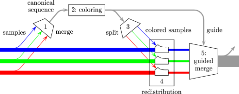
Figure 1: The five steps of Guidesort’s merge. Different colors or gray tones in the figure denote different runs and should not be confused with the colors used by Guidesort, which represent different disks.

A back-of-the-envelope estimate of the number of I/Os executed by Guidesort proceeds as follows: Steps 1–3 operate only on leaders and therefore have no significant I/O cost. Step 4 inputs all items and outputs them at half speed (because we can choose $\overline{D}\approx{D/2}$). Conversely, Step 5 inputs the items at half speed and outputs them at full speed. Altogether, each merge is about three times as expensive as would be inputting and outputting the relevant blocks once $D$ at a time. As a consequence, the complete sorting uses approximately $({3/D})\Tvn{Sort}_{M,B}(N)$ I/Os.

While the back-of-the-envelope estimate essentially leads to the correct result, a more precise argument must account for the cost of Steps 1–3, which is not always negligible, and must also work without a number of assumptions that were made implicitly above. This is the topic of the next two subsections.

2.2 A Realistic Simple Special Case

Define the block length of a stored sequence to be the number of block frames that it occupies (fully or in part). Let us be more specific about the recursive sorting algorithm, which is parameterized by an integer $r$ with $2\leq r\leq m$. When asked to sort a sequence of block length $p$, the algorithm first computes $k=\min\{\Tceil{{p/m}},r\}$. If $k=1$, the sorting takes place in the internal memory without recursive calls. Otherwise the input sequence is split into $k$ subsequences, each of block length $\Tfloor{{p/k}}$ or $\Tceil{{p/k}}$, and the $k$ subsequences are sorted recursively and subsequently merged. The main point is that although the algorithm “nominally” uses $r$-way merging, a call that issues terminal calls issues only as many as necessary. Without increasing the depth of the recursion, this ensures that each terminal call deals with at least $m/2$ blocks and therefore that the number of terminal calls and the number of calls altogether are $O({n/m})$. This is useful for dealing with rounding issues. E.g., if each merge executed as part of the overall sorting is associated with a quantity of the form $\Tceil{t}$, where $t$ is some expression, we can upper-bound the sum of $\Tceil{t}$ over all merges by summing $t$ over all merges and adding $O({n/m})$.

Our analysis frequently sums the number of I/Os of a particular kind over all merges carried out as part of the overall sorting. We shall use the term “accumulated” to denote this situation, i.e., “accumulated” means “summed over all merges”. Let $z$ be the accumulated total block length of the runs of all merges. Exactly as in the sequential sorting algorithm, $z\leq n\Tceil{\log_{r}\!n}$. Similarly, let $y$ be the accumulated block length of all samples produced by the algorithm. Since each leader in a sample “represents” $B$ items, an application of the counting method set out at the end of the previous paragraph shows that $y={z/B}+O({n/m})$.

Let $D_{1}=\min\{D,\Tfloor{m/2}\}\geq\max\{\Tfloor{D/2},1\}\geq{D/3}$. In the following, $D_{2}$, $D_{4}$, $D_{5}$ and $D\Tsub L$ are integers with $1\leq D_{2},D_{4},D_{5},D\Tsub L\leq D$ to be chosen later.

Step 1 merges at most $r$ samples. If the block length of some sample is $<m$, and therefore the block lengths of all samples are $\leq m$, the samples are first partitioned into bundles in such a way that the total block length of the runs in each bundle, except possibly the last bundle, is at least $m/2$ and at most $m$. The blocks in each bundle are then input, $D$ at a time, sorted internally, and output as one sorted sequence, again $D$ blocks at a time, at an accumulated cost of ${{2y}/D}+O({n/m})$ I/Os. Assume that the number of sorted runs (original samples or sorted bundles) at this point is $r^{\prime}$. The $r^{\prime}$ runs are merged in a binary merge tree of height $\Tceil{\log_{2}\!r^{\prime}}$ in which each binary merge is carried out with $D_{1}$ disks that operate in lock-step to simulate a single disk with a block size of $B^{\prime}=D_{1}B$.

Observe that ${n/m}\leq{n/D}=O(({z/D})({1/{\log_{m}\!n}}))$ (a convexity argument shows that we even have ${n/D}\leq({z/D})({1/{\log_{m}\!n}})$). When $r^{\prime}$ runs are merged in a binary merge tree, each run, except possibly the last one, contains at least $M/2$ leaders that “represent” at least ${{MB}/2}$ input items. With respect to a block size of $B^{\prime}$, the accumulated block length of all runs input to nontrivial binary merge trees—those with $r^{\prime}\geq 2$ leaves—is therefore $O({z/{(D_{1}B)}})=O({z/{(DB)}})$, and the merges can be carried out with $O({{z\Tceil{\log_{2}\!r}}/{(DB)}})=O({{(z\ln m)}/{(DB)}})$ I/Os. Altogether, the number of I/Os executed by Step 1 is $O({{(z\ln m)}/{(DB)}}+{n/m})$. This bound also covers Step 3, which reverses the merging to transfer the information attached to leaders in Step 2 from the guide to the samples. Steps 1 and 3 need $2D_{1}$ block frames of internal memory, which are available since $D_{1}\leq{m/2}$.

Step 2 colors the canonical sequence. Say that a color is used recently in a sequence of $k$ colored objects if it is the color of one of the $\min\{\overline{D}-1,k\}$ last objects in the sequence. The leaders are processed in the order in which they occur in the canonical sequence, and each leader $x$ is given a color in $\{0,\ldots,D-1\}$ that is used recently neither in the complete sorted sequence of colored leaders nor in its (not necessarily contiguous) subsequence of leaders drawn from the same sample as $x$. To accomplish its task, the algorithm maintains at most $r+1$ history sequences of the chronologically ordered recently used colors overall and within each sample. To process a leader, the algorithm identifies and assigns an appropriate color to the leader and updates two history sequences accordingly, all of which is straightforward. In addition, the leaders of each color are numbered consecutively in the order in which they are colored and the number of each leader, called its index, is attached to the leader. We will assume that the history sequences with their at most $(r+1)(\overline{D}-1)$ color values can be stored in $q=\Tceil{{(r+1)(\overline{D}-1)}/B}$ block frames. Using an additional input/output buffer of $D_{2}$ block frames, we can execute Step 2 with an accumulated number of I/Os of ${{2y}/{D_{2}}}+O({n/m})={{2z}/{(D_{2}B)}}+O({n/m})$. We must ensure that $q+D_{2}\leq m$.

Step 4 redistributes blocks to new disks one run at a time. When processing a run of $\ell$ blocks, the algorithm inputs the $\ell$ blocks and, interleaved, a sample of $\ell$ colored leaders and, for $i=1,\ldots,\ell$, stores the $i$th block on the disk corresponding to the color of the $i$th leader and in a block frame whose number is the index of the $i$th leader plus an offset chosen for that disk. Thus the blocks on each disk are stored compactly, but they are not necessarily written in the order of increasing frame numbers. With a “primary” input buffer of $D_{4}$ block frames for the input blocks, a “secondary” input buffer of $D\Tsub L$ block frames for the leaders and an output buffer of $\overline{D}$ block frames for the redistributed blocks, the accumulated number of I/Os spent in Step 4 is ${{z/{D_{4}}}}+{{z/{\overline{D}}}}+{y/{D\Tsub L}}+O({n/m})=z({1/{D_{4}}}+{1/{\overline{D}}}+{1/{(D\Tsub LB)}})+O({n/m})$. We must ensure that $D_{4}+\overline{D}+D\Tsub L\leq m$.

Step 5 actually merges the runs with the aid of one block frame of input buffer for each run, a total of at most $r$ block frames, an input buffer of $\overline{D}$ block frames for the latest batch ($\overline{D}-1$ block frames actually suffice), two buffers of $D\Tsub L$ block frames each for the guide, which is input, and the sample for the next recursive level, which is output, and finally a buffer of $D_{5}$ block frames for the primary output, the final outcome of the merge. The accumulated number of I/Os is ${{z/{\overline{D}}}}+{{z/{D_{5}}}}+2{{y/{D\Tsub L}}}+O({n/m})=z({1/{\overline{D}}}+{1/{D_{5}}}+{2/{(D\Tsub LB)}})+O({n/m})$, and we must ensure that $r+\overline{D}+D_{5}+2D\Tsub L\leq m$.

Collecting the contributions identified above and not forgetting the $O({n/D})$ I/Os consumed by terminal calls of the recursive sorting algorithm, we arrive at a total number of I/Os for the complete sorting of

$$z\left(\frac{1}{D_{4}}+\frac{1}{D_{5}}+\frac{2}{\overline{D}}+\frac{1}{B}\left(\frac{2}{D_{2}}+\frac{3}{D\Tsub L}\right)\right)+O\left(\frac{z\ln m}{DB}+\frac{n}{D}\right).$$ (1)

Assume that $m\geq 6D$, $B\geq D$ and $\ln m=o(B)$, conditions that are not unlikely to be met in a practical setting (of course, it is not really clear what $\ln m=o(B)$ is supposed to mean in a practical setting). Then we can satisfy all requirements identified in the discussion of Steps 2, 4 and 5 by taking $D_{2}=D_{4}=D_{5}=D\Tsub L=D$, $\overline{D}=\Tceil{D/2}$ and $r=m-4D\geq 2$ (in particular, $q\leq r+1$), and the total number of I/Os becomes at most $({z/D})(6+O({1/{\log_{m}\!n}})+o(1))$. Since $r\geq{m/3}$ and therefore $\ln m=(1+O({1/{\ln m}}))\ln r$, the number of I/Os can also be bounded by $({3/D})\Tvn{Sort}_{M,B}(N)(1+O({1/{\log_{m}\!n}})+o(1))$, where $n$ and $m$ are assumed to tend to infinity.

2.3 The General Case: An Order-of-Magnitude Bound

In order to deal with situations in which $B$ is smaller than $D$ or $\ln m$ is not small relative to $B$, we generalize the algorithm by introducing an additional parameter, $s$, which must be a positive divisor of $\overline{D}$. The algorithm described so far corresponds to the special case $s=1$.

Whereas until now a leader was the smallest item within a block, we redefine it to be the smallest item within a segment of $s$ consecutive blocks in some run. Thus each run is partitioned into segments of $sB$ items each, except that the last segment may be smaller, and each segment contributes only a single leader to the sample of the run. As a consequence, the accumulated block length of all samples now is $y={z/{(sB)}}+O({n/m})$. We stipulate that the $s$ blocks that form a segment are colored using consecutive colors that begin at a multiple of $s$. An intuitive view of this is that the task now is to color segments with one of ${{2\overline{D}}/s}-1$ colors so as to avoid the at most ${{\overline{D}}/s}-1$ most recent colors both overall and within the same run. This has the beneficial effect of reducing the state information that must be kept by the greedy coloring in Step 2 from $(r+1)(\overline{D}-1)$ colors to at most ${{(r+1)(\overline{D}-1)}/s}$ colors, which can be stored in $q=\Tceil{{{(r+1)(\overline{D}-1)}/{(sB)}}}$ blocks. On the other hand, in order for the leaders to fulfil their function, Step 5 must be changed to input runs whole segments at a time, which means that an input buffer of $s$ block frames rather than of a single block frame must be provided for each run. The requirement for Step 5 accordingly becomes $rs+\overline{D}+D_{5}+2D\Tsub L\leq m$ for the revised sorting algorithm, while the total number of I/Os generalizes from (1) to

$$z\left(\frac{1}{D_{4}}+\frac{1}{D_{5}}+\frac{2}{\overline{D}}+\frac{1}{sB}\left(\frac{2}{D_{2}}+\frac{3}{D\Tsub L}\right)\right)+O\left(\frac{z\ln m}{sDB}+\frac{n}{D}\right).$$ (2)

For $m\leq 3$ and therefore $D\leq 3$, sequential sorting obviously works within $({3/D})\Tvn{Sort}_{M,B}(N)$ I/Os. If $m\geq 4$ and $D\leq\sqrt{m}$, sorting by naive $\Tfloor{\sqrt{m}}$-way striping uses $({2/D})\Tvn{Sort}_{M,B}(N)(1+O({1/{\sqrt{m}}}))+O({n/D})$ I/Os. Both of these bounds are better than the bound claimed in Theorem 2.3 in the next subsection. We will therefore assume in the following that $D\geq\sqrt{m}$.

If the only goal is to prove a bound of $O(({1/D})\Tvn{Sort}_{M,B}(N))$, i.e., if constant factors are not considered significant, we can assume without loss of generality that $\sqrt{D}\geq 12$ and argue as follows: Take $s=\Tfloor{{{\sqrt{m}}/2}}\geq\Tfloor{{{\sqrt{D}}/2}}\geq 6$ and choose $\overline{D}$ as the largest multiple of $s$ bounded by $D/2$—which is $\Omega(D)$ since $s\leq{{\sqrt{m}}/2}\leq{D/2}$. Moreover, take $r=\Tfloor{s/2}-1\geq 2$ and $D_{2}=D_{4}=D_{5}=D\Tsub L=\Tfloor{D/8}\leq{m/8}$. It is now easy to see that the requirements of Steps 2, 4 and 5 are satisfied. In particular, $q=\Tceil{{{(r+1)(\overline{D}-1)}/{(sB)}}}\leq\Tceil{{{\overline{D}}/{(2B)}}}\leq\Tceil{{m/4}}$ and $rs\leq({1/2})({{\sqrt{m}}/2})^{2}={m/8}$. The number of I/Os executed by the algorithm is $O({z/D})$. Moreover, $r=\Omega(\sqrt{m})$ and therefore $\ln r=\Omega(\ln m)$, so the number of I/Os is indeed $O(({1/D})\Tvn{Sort}_{M,B}(N))$. If we want to prove a more precise bound, we must choose the parameters more carefully.

2.4 The General Case: Good Constant Factors

In order to obtain the best result, we change the algorithm slightly: In Step 4, instead of having separate primary input and output buffers of $D_{4}$ and $\overline{D}$ block frames, respectively, we use a single buffer of $D_{4}$ block frames for both input and output. This is trivial, but requires us to ensure that $\overline{D}\mid D_{4}$ (i.e., $\overline{D}$ divides $D_{4}$).

Besides $r$, $s$, $\overline{D}$, $D_{2}$, $D_{4}$, $D_{5}$ and $D\Tsub L$ being positive integers, the conditions that the parameters must satisfy for the final algorithm are the following:

$$\overline{D} \leq\Tceil{D/2}$$

$$D_{2},D_{4},D_{5},D\Tsub L \leq D$$

$${{(r+1)(\overline{D}-1)}/{(sB)}}+D_{2} \leq m$$

$$D_{4}+D\Tsub L \leq m$$ (3)

$$rs+\overline{D}+D_{5}+2D\Tsub L \leq m$$

$$2\leq r \leq m$$

$$s\mid\overline{D}\mbox{ and }\overline{D} \mid D_{4}.$$

Our task at this point is to (approximately) minimize the I/O bound of (2) subject to the constraints (3). As an aid in dealing with the divisibility requirements of the last constraint, we first prove a simple technical lemma that, informally, says that, given two positive integers $a$ and $b$, we can make the smaller divide the larger without changing their sorted order by lowering each by less than half and $b$ by less than its square root. Since we will actually use the lemma only with $a\leq\sqrt{b}$, it is more general than what is needed here. Let $\TbbbN=\{1,2,\ldots\}$.

Lemma 2.1.

There is a function $f:\TbbbN^{2}\to\TbbbN^{2}$ that can be evaluated in constant time and has the following properties: For all $a,b\in\TbbbN$, if $(a^{\prime},b^{\prime})=f(a,b)$, then

• $a^{\prime}\mid b^{\prime}$ or $b^{\prime}\mid a^{\prime}$;

• ${a/2}<a^{\prime}\leq a$;

• $\max\{{b/2},b-\sqrt{b}\}<b^{\prime}\leq b$;

• $(a-b)(a^{\prime}-b^{\prime})\geq 0$.

Proof 2.2.

If $a=1$, take $a^{\prime}=a$ and $b^{\prime}=b$. Otherwise, if $a\geq b$, take $a^{\prime}=\Tfloor{a/b}b>{a/2}$ and $b^{\prime}=b$. If $a=b-1\geq 2$, take $a^{\prime}=b^{\prime}=a>\max\{b/2,b-\sqrt{b}\}$. From now on assume that $2\leq a\leq b-2$. Since then $b\geq 4$ and $\sqrt{b}\leq{b/2}$, we need no longer verify the condition $b^{\prime}>{b/2}$ explicitly. Consider two cases:

If $a\leq\sqrt{b}+1$, take $a^{\prime}=a$ and $b^{\prime}=\Tfloor{b/a}a\leq b$ and observe that if $a<\sqrt{b}+1$, then $b^{\prime}=\Tfloor{b/a}a\geq b-a+1>b-\sqrt{b}$, whereas if $a=\sqrt{b}+1$, then $b^{\prime}=\Tfloor{b/a}a\geq\Tfloor{\sqrt{b}-1}(\sqrt{b}+1)=b-1>b-\sqrt{b}$.

If $\sqrt{b}+1<a\leq b-2$, take $a^{\prime}=\Tfloor{b/{\Tceil{b/a}}}\leq a$ and observe that if $a\geq{b/2}$, then $a^{\prime}=\Tfloor{b/2}\geq\Tfloor{{{(a+2)}/2}}>{a/2}$, whereas if $a<{b/2}$, then we can successively conclude that $a\geq 4$, $b\geq 9$ and $a\geq 5$ and then that $a^{\prime}\geq\Tfloor{b/{({b/a}+1)}}=\Tfloor{{ab}/{(b+a)}}\geq\Tfloor{{{2a}/3}}>{a/2}$. Also take

$$b^{\prime}=\Tceil{b/a}a^{\prime}=\Tceil{b/a}\left\lfloor{\frac{b}{\Tceil{b/a}}}\right\rfloor\geq b-\Tceil{b/a}+1\geq b-\Tceil{\sqrt{b}}+1>b-\sqrt{b}$$

and note that $b^{\prime}\leq b$ is obvious from the third expression in the previous line.

The stage is set for our main result:

Theorem 2.3.

For all positive integers $M$, $B$, $D$ and $N$ with $M\geq 2B$, $B\mid M$, $D\leq{M/B}$ and $N>M$, $N$ items can be sorted with internal memory size $M$, block size $B$ and $D$ disks with

$$\frac{(3+g({m/D}))h(\log_{m}({{8D}/B}))}{D}\cdot\Tvn{Sort}_{M,B}(N)(1+F^{\prime}(M,B,D,N))$$

I/Os, where $n=\Tceil{N/B}$, $m={M/B}$, $\Tvn{Sort}_{M,B}(N)=2n\Tceil{\log_{m}\!n}$,

$$g(x)={\frac{\max\{5-2x,0\}}{4x-2}}\leq{3/2}$$

for $x\geq 1$, $h(x)={1/{(1-({1/2})\max\{0,\min\{x,1\}\})}}\leq 2$ for arbitrary real $x$ and

$$F^{\prime}(M,B,D,N)=O\left(\frac{1}{\log_{m}\!n}+\frac{D}{m\ln m}+\frac{\ln m}{\sqrt{DB}}+\frac{1}{(DB)^{1/4}}+\frac{1}{\sqrt{D}}\right).$$

Proof 2.4.

Because of the term ${1/{\sqrt{D}}}$ in the expression for $F^{\prime}$, we can assume without loss of generality that $m$ is larger than a certain constant $m_{0}$, which we choose as $m_{0}=2^{12}$. As justified earlier, we will also assume that $D\geq\sqrt{m}$. We use the algorithm developed in the previous subsections and compute the parameter values as follows ($f$ is the function of Lemma 2.1, and $\widetilde{D}$, $r_{2}$ and $r_{5}$ are auxiliary quantities):

$\displaystyle D\Tsub L:=\left\lceil\frac{D}{4(DB)^{1/4}}\right\rceil$;

$\widetilde{D}:=\displaystyle\left\lfloor\frac{\min\{D,m-D\Tsub L\}}{2}\right\rfloor$;

$(s,\overline{D}):=f\left(\max\left\{\left\lfloor\sqrt{{{\widetilde{D}}/B}}\right\rfloor,1\right\},\widetilde{D}\right)$;

$D_{5}:=\displaystyle\min\left\{\left\lfloor\frac{m-\overline{D}-2D\Tsub L}{2}\right\rfloor,D\right\}$;

$r_{2}:=\displaystyle\left\lfloor\frac{(m-1)sB}{\overline{D}-1}\right\rfloor-1$;

$r_{5}:=\displaystyle\left\lfloor\frac{m-\overline{D}-D_{5}-2D\Tsub L}{s}\right\rfloor$;

$r:=\min\{\Tfloor{{{r_{2}}/2}},r_{5}\}$;

$D_{2}:=\displaystyle\min\left\{m-\left\lceil\frac{(r+1)(\overline{D}-1)}{sB}\right\rceil,D\right\}$;

$D_{4}:=2\overline{D}$;

Let $D\Tsub L$, etc., be the values computed above. Because $m\geq D$ and $m\geq 2^{8}$, $D\Tsub L\leq\Tceil{{m/{(4m^{1/4})}}}\leq\Tceil{{m/{16}}}\leq{m/8}$. Now $\widetilde{D}\geq\min\{\Tfloor{{D/2}},\Tfloor{({7/{16}})m}\}$, which is at least 2 because $D\geq 4$ and $m\geq 5$. By the third property of Lemma 2.1, we also have $\overline{D}\geq 2$. Hence the computation of $r_{2}$ does not lead to a division by zero and since $s\geq 1$, all other steps are easily seen to be well-defined.

We first argue that the constraints (3) are satisfied. All values computed are integers. First, $1\leq\overline{D}\leq\widetilde{D}\leq\Tfloor{D/2}\leq\Tceil{D/2}$. Then, clearly, $D_{2},D_{4},D_{5},D\Tsub L\leq D$. The relation ${{(r+1)(\overline{D}-1)}/{(sB)}}+D_{2}\leq m$ holds because $D_{2}$ is computed precisely as the largest integer solution bounded by $D$ to this (linear) inequality. Similarly, $r_{5}s+\overline{D}+D_{5}+2D\Tsub L\leq m$ and $rs+\overline{D}+D_{5}+2D\Tsub L\leq m$ hold because $r_{5}$ is computed as the largest integer solution to the first inequality and $r\leq r_{5}$. Moreover, $D_{4}+D\Tsub L=2\overline{D}+D\Tsub L\leq 2\widetilde{D}+D\Tsub L\leq m$. To see that $D_{2}\geq 1$, it suffices to observe that ${{(r_{2}+1)(\overline{D}-1)}/{(sB)}}\leq m-1$ and that $r\leq r_{2}$. We have $D_{5}\geq 1$ because $m-\overline{D}-2D\Tsub L\geq{m/4}$ and $m\geq 8$. Since the first argument of $f$ is no larger than its second argument, the first and last properties of Lemma 2.1 show that $s\mid\overline{D}$. It is easy to see that $D_{4}\geq 1$, $\overline{D}\mid D_{4}$ and $r\leq m$.

What remains is to prove that $r\geq 2$ or, equivalently, that $r_{2}\geq 4$ and $r_{5}\geq 2$. First,

$$\left\lfloor\sqrt{{\widetilde{D}}/{B}}\right\rfloor\geq\left\lfloor\sqrt{\frac{\Tfloor{({7/{16}})D}}{B}}\right\rfloor=\left\lfloor\sqrt{\frac{7D}{16B}}\right\rfloor$$

and hence, by the second property of Lemma 2.1, $s\geq({1/2})\sqrt{{{7D}/{(16B)}}}$. Now ${{(m-1)sB}/{(\overline{D}-1)}}\geq 2sB\geq\sqrt{{{7D}/{16}}}\geq 5$, where the last inequality follows from $D\geq\sqrt{m}\geq 2^{6}$, and this shows that $r_{2}\geq 4$.

In order to demonstrate that $r_{5}\geq 2$, we prove that $m-\overline{D}-D_{5}-2D\Tsub L\geq 2s$. Briefly let $u=m-\overline{D}-2D\Tsub L$. Since $D_{5}\leq\Tfloor{{u/2}}$, $m-\overline{D}-D_{5}-2D\Tsub L=u-D_{5}\geq\Tceil{{u/2}}$. But

$$u\geq m-\left\lfloor\frac{m-1}{2}\right\rfloor-\frac{m}{4}=m-1-\left\lfloor\frac{m-1}{2}\right\rfloor+\frac{4-m}{4}=\left\lceil\frac{m+2}{4}\right\rceil.$$

It therefore suffices to show that ${{(m+2)}/8}>2s-1$ or that $m>16s-10$. But since $s\leq\sqrt{D}\leq\sqrt{m}$, this follows from $m\geq 2^{8}$.

We next bound the number of I/Os executed by the algorithm, essentially by estimating the values of its parameters. First

$$D\Tsub L=\left\lceil\frac{D}{4(DB)^{1/4}}\right\rceil=O\left(D\left(\frac{1}{(DB)^{1/4}}+\frac{1}{D}\right)\right)$$

and therefore

$$\widetilde{D}=D\left(\frac{1}{2}-O\left(\frac{1}{(DB)^{1/4}}+\frac{1}{D}\right)\right).$$

By the third property of Lemma 2.1, it follows that

$$\overline{D}=D\left(\frac{1}{2}-O\left(\frac{1}{(DB)^{1/4}}+\frac{1}{\sqrt{D}}\right)\right).$$

As observed earlier, ${{(m-1)sB}/{(\overline{D}-1)}}\geq r_{2}+1$. But $r_{2}+1\geq 2r+1\geq({3/2})(r+1)$ and therefore ${{(r+1)(\overline{D}-1)}/{(sB)}}\leq({2/3})(m-1)$. As a consequence, $D_{2}=\Omega(D)$. Because $D_{4}$ is just $2\overline{D}$,

$$D_{4}=D\left(1-O\left(\frac{1}{(DB)^{1/4}}+\frac{1}{\sqrt{D}}\right)\right).$$

Noting that

$$2g(x)+1=\max\left\{\frac{10-4x+4x-2}{4x-2},1\right\}=\max\left\{\frac{1}{{x/2}-{1/4}},1\right\}$$

for $x\geq 1$, we find that

$$D_{5} =\displaystyle\min\left\{\left\lfloor\frac{m-\overline{D}-2D\Tsub L}{2}\right\rfloor,D\right\}$$

$$\geq D\left(\min\left\{\frac{m}{2D}-\frac{1}{4},1\right\}-O\left(\frac{1}{(DB)^{1/4}}+\frac{1}{D}\right)\right)$$

$$=D\left(\frac{1}{2g({m/D})+1}-O\left(\frac{1}{(DB)^{1/4}}+\frac{1}{D}\right)\right).$$

We are almost ready to sum the terms in (2). Observe first that since $D_{4}$, $D_{5}$ and $\overline{D}$ are all larger than $\epsilon D$ for some fixed $\epsilon>0$, our bound of the form $D_{4}=D(1-O(\cdots))$ yields a bound of the form ${1/{D_{4}}}=({1/D})(1+O(\cdots))$, and analogously for $D_{5}$ and $\overline{D}$. We already noted that $sB=\Omega(\sqrt{DB})$. Hence

$$\frac{1}{sB}\left(\frac{2}{D_{2}}+\frac{3}{D\Tsub L}\right)=O\left(\frac{1}{\sqrt{DB}}\cdot\frac{1}{D}\left(1+{(DB)^{1/4}}\right)\right)=O\left(\frac{1}{D}\cdot\frac{1}{(DB)^{1/4}}\right).$$

We also have

$$\frac{z\ln m}{sDB}+\frac{n}{D}=O\left(\frac{z}{D}\left(\frac{\ln m}{\sqrt{DB}}+\frac{1}{\log_{m}\!n}\right)\right).$$

Now the total number of I/Os can be seen to be

$$z \left(\frac{1}{D_{4}}+\frac{1}{D_{5}}+\frac{2}{\overline{D}}+\frac{1}{sB}\left(\frac{2}{D_{2}}+\frac{3}{D\Tsub L}\right)\right)+O\left(\frac{z\ln m}{sDB}+\frac{n}{D}\right)$$

$$=\frac{z}{D} \left(6+2g({m/D})+O\left(\frac{1}{\log_{m}\!n}+\frac{\ln m}{\sqrt{DB}}+\frac{1}{(DB)^{1/4}}+\frac{1}{\sqrt{D}}\right)\right).$$

By the second property of Lemma 2.1, $s\geq({1/2})\sqrt{{{\widetilde{D}}/B}}\geq({1/2})\sqrt{{{\overline{D}}/B}}$ and therefore ${{msB}/{\overline{D}}}\geq({m/2})\sqrt{{B/{\overline{D}}}}\geq m\sqrt{{B/{(2D)}}}$ and $\Tfloor{{r_{2}}/2}\geq m\sqrt{{B/{(8D)}}}-O(1)$. Since $r_{2}=\Omega(\sqrt{m})$, this implies that

$$\ln(\Tfloor{{r_{2}}/2})\geq\ln m-({1/2})\ln({{8D}/B})-O({1/{\sqrt{m}}}).$$

Similarly, $s\leq\max\{\sqrt{{D/B}},1\}$ and therefore

$$r_{5}\geq{\frac{\max\{m-2D,{m/4}\}}{\max\{\sqrt{{D/B}},1\}}}-O(1).$$

We essentially already observed that $r_{5}\geq\Tfloor{{\sqrt{m}}/8}=\Omega(\sqrt{m})$, so

$$\ln r_{5} \geq\ln(\max\{m-2D,{m/4}\})-\max\{({1/2})\ln({D/B}),0\}-O({1/{\sqrt{m}}})$$

$$=\ln m-\max\{({1/2})\ln({D/B}),0\}-O({D/m}).$$

Since $r=\min\{\Tfloor{{r_{2}}/2},r_{5}\}$, we may conclude that

$$\ln r \geq\ln m-\max\{({1/2})\ln({{8D}/B}),0\}-O({D/m})$$

$$=\ln m-({1/2})\max\{0,\min\{\ln({{8D}/B}),\ln m\}\}-O({D/m}).$$

and

$$\frac{\ln m}{\ln r} \leq\frac{1}{1-({1/2})\max\{0,\min\{\log_{m}({{8D}/B}),1\}\}}+O\left(\frac{D}{m\ln m}\right)$$

$$={{h(\log_{m}({8D}/B))}}+O\left(\frac{D}{m\ln m}\right).$$

Since

$$z\leq\Tvn{Sort}_{M,B}(N){\frac{\ln m}{2\ln r}}\left(1+\frac{1}{\log_{m}\!n}\right),$$

the total number of I/Os can therefore also be bounded by

$$\frac{(3+g({m/D}))h(\log_{m}({D/B}))}{D}\cdot\Tvn{Sort}_{M,B}(N)\left(1+F^{\prime}(M,B,D,N)\right),$$

where $F^{\prime}$ is as in the theorem.

Remark 2.5.

No attempt was made to use the smallest possible $m_{0}$ in the first part of the proof of Theorem 2.3. The assumption $m\geq m_{0}=2^{12}$ can be replaced by $m\geq 8$, $D\geq 4$ (but still also $D\geq\sqrt{m}$) and $B\geq 16$, which excludes only cases of scant practical interest. To show this, we revise the first part of the proof of Theorem 2.3 and provide new justification for the claims proved using the large value of $m_{0}$. Hence assume that $m\geq 8$, $D\geq 4$ and $B\geq 16$ and note that $B^{1/4}\geq 2$.

The first claim to reprove is that $D\Tsub L\leq{m/8}$. This holds for $m\leq 16$ because $D^{3/4}\leq m^{3/4}\leq 8$ and therefore $D\Tsub L\leq\Tceil{({1/8})D^{3/4}}=1\leq{m/8}$ and for $m\geq 16$ because $m^{1/4}\geq 2$ and therefore $D\Tsub L\leq\Tceil{({1/8}){m/{m^{1/4}}}}\leq\Tceil{{m/{16}}}\leq{m/8}$.

To show that $r_{2}\geq 4$, the proof of Theorem 2.3 argued that $2sB\geq 5$, a relation that is a triviality for $B\geq 16$. In the case of $r_{5}\geq 2$, the relation to show was $m>16s-10$. But for $8\leq m\leq 16$ this is clear since $s=1$, while for $m\geq 16$ it follows from $s\leq\sqrt{{D/B}}\leq({1/4})\sqrt{m}$.

It is easy to see that the asymptotic assertions of Theorem 2.3 continue to hold.

If $m\geq({5/2})D$, $g({m/D})=0$, and if $B\geq 8D$, $h(\log_{m}({{8D}/B}))=1$. If both of the conditions $m\geq({5/2})D$ and $B\geq 8D$ are satisfied, therefore, the quantity $(3+g({m/D}))h(\log_{m}({{8D}/B}))$ of Theorem 2.3 is 3. On the other hand, it is never larger than $(3+{3/2})\cdot 2=9$.

3 Conclusion

Guidesort is simple and based on a natural idea. If a reasonably programmed algorithm for sorting through multiway merging is available, the new algorithm can be grafted onto it by replacing the old subroutine for multiway merging by one that executes Steps 1–5. Step 1 is standard merging. Because the sequences to be merged are smaller by a factor of $B$ than the actual runs, in many practical situations the merging can be done any which way. The algorithm proposed here that can be viewed as the final part of sorting by naive 2-way striping is also very easy to implement. Step 3 is an even simpler approximately inverse operation. Step 5 is standard merging, except that the tests to identify the disks from which to input the next blocks have been executed beforehand. Step 2 implements a straightforward greedy algorithm, and Step 4 is a trivial redistribution of blocks according to a precomputed pattern.

While most or all previous algorithms are optimal with respect to internal computation, i.e., execute $O(N\ln N)$ steps of internal computation to sort $N$ items, it is not obvious how to carry out the greedy coloring of our Step 2 in less than $\Theta({{\overline{D}}/s})$ time per block (or $\Theta({{\overline{D}}/{(sw)}}+1)$ time per block if $w$ bits can be manipulated together in constant time), for which reason we can bound the amount of internal computation of Guidesort only by $O(N\ln N+({{nD}/s})\log_{m}\!n)=O(N(\ln N+\sqrt{{D/B}}\log_{m}\!n))$. For most realistic parameter values, however—in particular, if $D\leq B$—this is still $O(N\ln N)$.

It may seem deplorable that the function $F^{\prime}$ should include an “error term” of $O({1/{\log_{m}\!n}})$, which can be quite large even for realistic values of the parameters $n$ and $m$. However, recall that the term represents just $O({n/D})$ I/Os, i.e., the cost of a single pass over the input at full parallel speed. Approximating the total depth of the leaves in the recursion tree of a bottom-up or top-down algorithm similar to those published to date by $\Tceil{\log_{m}\!n}$ times the number of leaves incurs an error of the same magnitude. An “error” of $O({n/m})$, which is comparable if $D\approx m$, seems even harder to avoid: The number of nodes in the recursion tree is $\Theta({n/m})$, so if $\Omega(1)$ I/Os are “lost” on average at every node, e.g., because of a last block that is only partially occupied by items, the accumulated waste amounts to $\Omega({n/m})$ I/Os.

References

- [1] Alok Aggarwal and C. Greg Plaxton. Optimal parallel sorting in multi-level storage. In Proc. 5th Annual ACM–SIAM Symposium on Discrete Algorithms (SODA 1994). Arlington, Virginia, USA, pages 659–668, 1994.
- [2] Alok Aggarwal and Jeffrey Scott Vitter. The input/output complexity of sorting and related problems. Commun. ACM, 31(9):1116–1127, 1988.
- [3] Rakesh D. Barve, Edward F. Grove, and Jeffrey Scott Vitter. Simple randomized mergesort on parallel disks. Parallel Comput., 23(4–5):601–631, 1997.
- [4] Roman Dementiev and Peter Sanders. Asynchronous parallel disk sorting. In Proc. 15th Annual ACM Symposium on Parallelism in Algorithms and Architectures (SPAA 2003), San Diego, California, USA, pages 138–148, 2003.
- [5] Michael L. Fredman and Michael E. Saks. The cell probe complexity of dynamic data structures. In Proc. 21st Annual ACM Symposium on Theory of Computing (STOC 1989), Seattle, Washington, USA, pages 345–354, 1989.
- [6] David A. Hutchinson, Peter Sanders, and Jeffrey Scott Vitter. Duality between prefetching and queued writing with parallel disks. SIAM J. Comput., 34(6):1443–1463, 2005.
- [7] Donald E. Knuth. The Art of Computer Programming, Volume 3: Sorting and Searching. Addison-Wesley, Reading, Massachusetts, USA, 1973.
- [8] Vamsi Kundeti and Sanguthevar Rajasekaran. Efficient out-of-core sorting algorithms for the Parallel Disks Model. J. Parallel Distrib. Comput., 71(11):1427–1433, 2011.
- [9] Tom Leighton. Tight bounds on the complexity of parallel sorting. IEEE Trans. Comput., 34(4):344–354, 1985.
- [10] Mark H. Nodine and Jeffrey Scott Vitter. Deterministic distribution sort in shared and distributed memory multiprocessors. In Proc. 5th Annual ACM Symposium on Parallel Algorithms and Architectures (SPAA 1993), Velen, Germany, pages 120–129, 1993.
- [11] Mark H. Nodine and Jeffrey Scott Vitter. Greed Sort: Optimal deterministic sorting on parallel disks. J. ACM, 42(4):919–933, 1995.
- [12] Sanguthevar Rajasekaran and Sandeep Sen. Optimal and practical algorithms for sorting on the PDM. IEEE Trans. Comput., 57(4):547–561, 2008.
- [13] Jeffrey Scott Vitter and David Alexander Hutchinson. Distribution sort with randomized cycling. J. ACM, 53(4):656–680, 2006.
- [14] Jeffrey Scott Vitter and Elizabeth A. M. Shriver. Algorithms for parallel memory, I: Two-level memories. Algorithmica, 12(2/3):110–147, 1994.