Kernel Density Estimation-Based
Markov Models with Hidden State

Abstract

We consider Markov models of stochastic processes where the next-step conditional distribution is defined by a kernel density estimator (KDE), similar to Markov forecast densities and certain time-series bootstrap schemes. The KDE Markov models (KDE-MMs) we discuss are nonlinear, nonparametric, fully probabilistic representations of stationary processes, based on techniques with strong asymptotic consistency properties. The models generate new data by concatenating points from the training data sequences in a context-sensitive manner, together with some additive driving noise. We present novel EM-type maximum-likelihood algorithms for data-driven bandwidth selection in KDE-MMs. Additionally, we augment the KDE-MMs with a hidden state, yielding a new model class, KDE-HMMs. The added state variable captures non-Markovian long memory and signal structure (e.g., slow oscillations), complementing the short-range dependences described by the Markov process. The resulting joint Markov and hidden-Markov structure is appealing for modelling complex real-world processes such as speech signals. We present guaranteed-ascent EM-update equations for model parameters in the case of Gaussian kernels, as well as relaxed update formulas that greatly accelerate training in practice. Experiments demonstrate increased held-out set probability for KDE-HMMs on several challenging natural and synthetic data series, compared to traditional techniques such as autoregressive models, HMMs, and their combinations.

1 Introduction

Time series and other sequence data are ubiquitous in nature. To recognize patterns or make decisions based on observations in the face of uncertainty and natural variation, or to generate new data, e.g., for synthesizing speech, we need capable stochastic models.

Exactly what model to use depends on the situation. The standard approach is to propose a mathematical framework, and then let data fill in the unknowns by estimating parameters [1, 2]. If the data-generating process is well understood, it may be possible to write down an appropriate model form directly. If not, we must fall back on the extensive library of general-purpose statistical models available. With little data, simple, tried-and-true approaches are typically used. These tend to involve many assumptions on the nature of the data-generating process. Model accuracy may suffer if these assumptions are incorrect. Once more data becomes available, such as in today’s “big data” paradigm, it is often possible to get a better description by fitting more advanced models with additional parameters. Using a complex model is certainly no guarantee for better results, however, and finding out which particular description to use tends to be a laborious trial-and-error process.

In this article, we consider a class of nonparametric models for discrete-time, continuous-valued stationary data series, where conditional next-step distributions are defined by kernel density estimators. Unlike standard parametric techniques, these models can converge on a significantly broader class of ergodic finite-order Markov processes as the training data material grows large. This makes the models widely applicable, and is especially compelling for data where the generating process is complex and nonlinear, or otherwise poorly understood.

Our main contributions are 1) extending the nonparametric Markov models with a discrete-valued hidden state, and 2) presenting several guaranteed-ascent iterative update formulas for maximum-likelihood parameter estimation, applicable both with and without hidden state. The added state variable allows models to capture long-range dependences, patterns with variable duration, and similar structure, on top of the short-range correlations described by the Markov model. This is shown to improve finite-sample performance on challenging real-world data. The state variable can also be used as an input signal to control process output, and is attractive for recognition and synthesis applications, particularly with speech signals, where the hidden states can be identified with language units such as phones.

The remainder of the paper is organized as follows: Section 2 discusses established techniques for modelling Markovian processes with and without hidden state, along with sample applications. Section 3 then introduces kernel density-based time series models and their properties. Parameter estimation is subsequently treated in Section 4. Sections 5 and 6 present experimental results, while Section 7 concludes.

2 Background

In this section we discuss Markov models and hidden-state models for strictly stationary and ergodic sequence data, and also address how the two approaches can be combined to describe more complex natural processes.

2.1 Markov Models

Let the underline notation $\underline{X}_{1}^{T}=\left(X_{1},\,\ldots,\,X_{T}\right)$ represent a sequence of variables from a stochastic process. A process satisfying

$$f_{X_{t}\;|\;\underline{X}_{-\infty}^{t-1}}\left(x_{t}\;|\;\underline{x}_{-\infty}^{t-1}\right) \equiv f_{X_{t}\;|\;\underline{X}_{t-p}^{t-1}}\left(x_{t}\;|\;\underline{x}_{t-p}^{t-1}\right)\textrm{;}$$ (1)

is said to be a Markov process of order $p$. The relation implies that future evolution is conditionally independent of the past, given the latest observations—the context or state $\underline{x}_{t-p}^{t-1}$. In other words, the process has a short, finite memory, and knowing the most recent samples suffices for optimal prediction. $p=0$ means that variables are independent. The Bayesian network in Fig. 1a illustrates the between-variable dependences when $p=2$.

Continuous-valued Markovian data can be modelled using linear as well as nonlinear models. Standard linear autoregressive (AR) and autoregressive moving-average (ARMA) models are perhaps the most well-known. Among nonlinear models one finds piecewise-linear, regime-switching approaches such as self-exciting threshold autoregressive (SETAR) models [3], non-recurrent time-delay neural networks (TDNN) [4], or kernel-based AR models [5, 6]. Similar to regular AR models, the latter can be made probabilistic by exciting them with a random process, typically white noise.

All the above models are parametric, and can therefore only converge on processes in their finite-dimensional parametric family. This may limit the achievable accuracy. As it turns out, convergent, general-purpose models are possible using nonparametric techniques. In Section 3 we highlight and extend a simple but flexible approach based on kernel density estimation, drawing on [7] and [8]. The technique is asymptotically consistent for stationary and ergodic Markov processes [10] despite having only a single free parameter, and outperforms traditional methods on multiple datasets.

2.2 Hidden-State Models

To capture long-range dependences, a Markov model may require a high order, many parameters, and a large dataset to provide a reasonable description. A more efficient approach is to use models with a hidden, unobservable state variable $Q_{t}$ that governs time-series evolution. The state is assumed to follow a Markov process, while the observed process values, in turn, are stochastic functions $f_{X_{t}\;|\;Q_{t}}$ of the current state alone. This dependence structure is illustrated in Fig. 1b. In this framework, discrete state spaces lead to hidden Markov models (HMMs) [11] and variants thereof, while continuous state spaces yield Kalman filters [12] and nonlinear extensions such as those presented in [13] and [14].

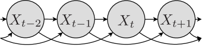
(a) Second-order Markov model.

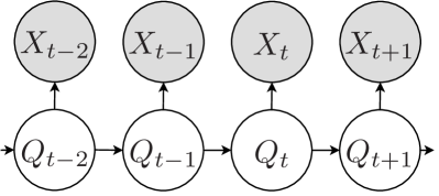
(b) Model with hidden state.

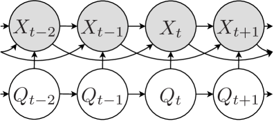
(c) Combined model.

Figure 1: Variable dependences in various sequence models. $X$s denote observed process values while $Q$s are unobserved (hidden) state variables.

Even though the hidden state $\underline{Q}$ satisfies the Markov property, the distribution of the observed data $\underline{X}$ typically cannot be represented by any finite-order Markov process. This is clear, e.g., from the forward algorithm

$$f_{Q_{t}\;|\;\underline{X}_{t_{0}}^{t}}\left(q\;|\;\underline{x}_{t_{0}}^{t}\right)\propto f_{X_{t}\;|\;Q_{t}}\left(x_{t}\;|\;q\right)\\ \cdot\sum_{q^{\prime}}P\left(Q_{t}=q\;|\;Q_{t-1}=q^{\prime}\right)f_{Q_{t-1}\;|\;\underline{X}_{t_{0}}^{t-1}}\left(q^{\prime}\;|\;\underline{x}_{t_{0}}^{t-1}\right)$$ (2)

for state inference in HMMs [11], which recursively depends on all previous samples. Hidden-state models can thus integrate predictive information over arbitrary lengths of time, providing efficient representations of long-range signal structure such as, for instance, the order of sounds in speech signals or different chart patterns in financial technical analysis. At the same time, efficient inference is possible for HMMs using the forward-backward algorithm [11].

Like the components in a mixture model, the discrete state of hidden-Markov models essentially partitions the data into different subsets, each explained by a different distribution. This can capture more detail in the data distribution than can a single component. HMMs furthermore model how components correlate across time, making them capable of representing series data.

2.3 Combined Models

Real-world data series often exhibit both short-range correlations and long-range structure. In theory, this can be represented by a discrete-state HMM given a sufficient number of states, but in practice that number may be prohibitively large. We see that HMMs trade the limited memory range of Markov models for a limited memory resolution (a finite state space).

To get the best of both worlds, Markovian observation dependences and hidden-state dynamics can be combined within a single model. This results in a model structure as illustrated in Fig. 1c, where between-sample dependences follow a Markov process with properties determined by the hidden state. Such a structure is seen in, e.g., GARCH models [15] from econometrics, or in SETAR models driven by an unobservable Markov chain (so-called Markov switching models [16, 3]). The addition of dynamic features (velocity and acceleration) to ordinary HMMs—a common practice in acoustic modelling of speech [17]—can be viewed as a method for adding implicit between-frame correlations. Autoregressive HMMs (AR-HMMs) [18] and trajectory HMMs [19] are similar models that make these dependences explicit. We will use AR-HMMs as a baseline since they are based on standard AR models and have a directed structure that allows efficient sampling and parameter estimation.

The Markovian part in a combined model typically captures simple and predictable local aspects of the data, such as continuity, allowing the hidden state to concentrate on more complex, long-range interactions. In acoustic modelling of speech, e.g., [19, 20], dynamic features capture correlations between analysis frames due to physical constraints on the motion of speech articulators, while the hidden states are based on a language model (e.g., $n$-grams) and account for grammar and other large-scale language structures.

As a major contribution of this article, we extend kernel density-based Markov models as used in [21, 8] with a hidden state. This is found to improve the distribution-prediction performance for held-out data over comparable parametric approaches such as AR-HMMs.

3 KDE Models for Time Series

In this section, we first review kernel density estimation of probability distributions, and how it can be adapted to describe and generate Markovian processes. Novel models with hidden state are introduced in Section 3.5.

From now on, we will use the letters $y$ and $x$ to denote training data and test data, respectively. $\mathcal{D}$ represents a set of training data, e.g., a training data sequence $\mathcal{D}=\underline{y}_{1}^{N}$, while boldface signifies vector-valued variables.

3.1 Kernel Density Estimation

Kernel density estimation (KDE) or Parzen estimation, introduced in [22, 23] and discussed in more detail in [24], is a nonparametric method for estimating a $D$-dimensional probability density $f_{\boldsymbol{X}}$ from a finite sample $\mathcal{D}=\left\{\boldsymbol{y}_{n}\right\}_{n=1}^{N}$, $\boldsymbol{y}_{n}\in\mathbb{R}^{D}$, by convolving the empirical density function with a kernel function $k\left(\boldsymbol{r}\right)$. The resulting estimated pdf can be written as

$$\widehat{f}_{\boldsymbol{X}}\left(\boldsymbol{x}\;|\;\mathcal{D};\,h\right) =\frac{1}{N}\sum_{n=1}^{N}\frac{1}{h^{D}}k\left(\frac{1}{h}\left(\boldsymbol{x}-\boldsymbol{y}_{n}\right)\right)\textrm{,}$$ (3)

where the bandwidth $h>0$ is a scale parameter adjusting the width of the kernel.

We see that the KDE in (3) always defines a proper density if we require that $k\left(\boldsymbol{r}\right)\geq 0$ and that $k\left(\boldsymbol{r}\right)$ integrates to one. For technical reasons we also require the first moment $\int\boldsymbol{r}k\left(\boldsymbol{r}\right)\mathrm{d}\boldsymbol{r}$ to be zero and that the second moment $\int\boldsymbol{r}\boldsymbol{r}^{\intercal}k\left(\boldsymbol{r}\right)\mathrm{d}\boldsymbol{r}$ is bounded. A wide variety of kernels exists, with the squared-exponential or Gaussian kernel

$$k\left(\boldsymbol{r}\right) =\frac{1}{\sqrt{2\pi}}\exp\left(-\frac{1}{2}\boldsymbol{r}^{\intercal}\boldsymbol{r}\right)$$ (4)

being a common example. For simplicity, we generally assume that the kernel factors across dimensions as

$$k\left(\boldsymbol{r}\right) =\prod_{d=1}^{D}k_{d}\left(r_{d}\right)\textrm{;}$$ (5)

this is known as a product kernel. Furthermore, we often take all component functions $k_{d}\left(\cdot\right)$ to be identical.

The bandwidth $h$ controls the degree of smoothing the KDE applies to the empirical distribution function. Bandwidth selection, the task of choosing this $h$, is key to KDE performance. With an appropriate adaptive bandwidth selection scheme, such that $h\to 0$ while $Nh^{D}\to\infty$ as $N\to\infty$, KDE can be shown to converge asymptotically on the true probability density function in a mean-squared error sense, regardless of $k$. (Kernel shape $k\left(\cdot\right)$ is less important, with many standard choices yielding near-optimal performance [25].) Essentially, given an ever-growing collection of progressively more localized basis functions with centres drawn from $f_{\boldsymbol{X}}$, we can eventually represent arbitrarily small details in the pdf. Moreover, KDE attains the best possible convergence rate for nonparametric estimators [26], assuming optimal bandwidth selection.

In practice, KDE finite-sample performance depends heavily on the data and the particular bandwidth chosen. Smooth distributions are typically easy to learn and can use large $h$, whereas complicated distributions require more data and narrow bandwidths to bring out the details. Consequently, there are many techniques for choosing the bandwidth in a data-driven manner: see, e.g., [27] or [28] for reviews.

3.2 Kernel Conditional Density Estimation

We now consider how to approximate Markov processes. Using the Markov property (1), the density function for a univariate sequence $\underline{x}_{1}^{T}$ from a general stationary nonlinear Markov process of order $p$ can be written

$$f_{\underline{X}_{1}^{T}}(\underline{x}_{1}^{T})=f_{\underline{X}_{1}^{p}}\left(\underline{x}_{1}^{p}\right)\prod_{t=p+1}^{T}f_{X_{p+1}\;|\;\underline{X}_{1}^{p}}\left(x_{t}\;|\;\underline{x}_{t-p}^{t-1}\right)\textrm{.}$$ (6)

It is sufficient to specify the stationary conditional next-step distribution $f_{X_{p+1}\;|\;\underline{X}_{1}^{p}}$ to uniquely determine the $x$-process and its associated stationary distribution $f_{\underline{X}_{1}^{p}}$. A key idea in this paper is to use KDEs, specifically kernel conditional density estimation (KCDE), to estimate this conditional distribution from data.

Given two variables $\boldsymbol{X}\in\mathbb{R}^{D}$ and $\boldsymbol{X}^{\prime}\in\mathbb{R}^{D^{\prime}}$ and a kernel density estimate $\widehat{f}_{\boldsymbol{X},\,\boldsymbol{X}^{\prime}}\left(\boldsymbol{x},\,\boldsymbol{x}^{\prime}\right)$ of their joint distribution $f_{\boldsymbol{X},\,\boldsymbol{X}^{\prime}}$ from training data pairs $\left\{\left(\boldsymbol{y}_{n},\,\boldsymbol{y}^{\prime}_{n}\right)\right\}_{n=1}^{N}$, the estimate $\widehat{f}_{\boldsymbol{X},\,\boldsymbol{X}^{\prime}}$ also induces a conditional distribution

$$\widehat{f}_{\boldsymbol{X}\;|\;\boldsymbol{X}^{\prime}}\left(\boldsymbol{x}\;|\;\boldsymbol{x}^{\prime};\,h,\,h^{\prime}\right)=\frac{\widehat{f}_{\boldsymbol{X},\,\boldsymbol{X}^{\prime}}\left(\boldsymbol{x},\,\boldsymbol{x}^{\prime};\,h,\,h^{\prime}\right)}{\int\widehat{f}_{\boldsymbol{X},\,\boldsymbol{X}^{\prime}}\left(\boldsymbol{\xi},\,\boldsymbol{x}^{\prime};\,h,\,h^{\prime}\right)\mathrm{d}\boldsymbol{\xi}}$$ (7)

$$=\sum_{n=1}^{N}\frac{k_{\boldsymbol{X}^{\prime}}\left(\frac{\boldsymbol{x}^{\prime}-\boldsymbol{y}_{n}^{\prime}}{h^{\prime}}\right)}{\sum_{n^{\prime}=1}^{N}k_{\boldsymbol{X}^{\prime}}\left(\frac{\boldsymbol{x}^{\prime}-\boldsymbol{y}_{n^{\prime}}^{\prime}}{h^{\prime}}\right)}\frac{1}{h^{D}}k_{\boldsymbol{X}}\left(\frac{\boldsymbol{x}-\boldsymbol{y}_{n}}{h}\right)$$ ; (8)

this is the KCDE for $f_{\boldsymbol{X}\;|\;\boldsymbol{X}^{\prime}}$ [21, 10, 29]. (We have assumed that the kernel factors between $\boldsymbol{X}$ and $\boldsymbol{X}^{\prime}$.)

The estimator in (8) is (MSE) consistent if bandwidths satisfy $h,\,h^{\prime}\to 0$ and $Nh^{D}h^{\prime D^{\prime}}\to\infty$ when $N\to\infty$. As always, this flexibility and consistency comes at a price of increased computational complexity and memory demands over parametric approaches, since all $N$ data points typically must be stored and used in calculations, making, e.g., bandwidth selection scale as $N^{2}$. Fortunately, approximate $k$-nearest neighbour techniques can be used to accelerate KDE computations. Reference [30] describes a method based on dual trees yielding speedup factors up to six orders of magnitude for KDE likelihood computation on 10,000 points from a nine-dimensional census dataset.

3.3 KDE Markov Models

Let $\underline{y}_{1}^{N}$ be a sampled data sequence (time series) from a stationary, ergodic Markov process of interest. Since $\underline{y}_{1}^{N}$ can be seen as a set of samples $\mathcal{D}=\left\{\underline{y}_{n-p}^{n}\right\}_{n=p+1}^{N}$ from the stationary distribution of $\underline{X}_{1}^{p+1}$, we can apply KCDE to estimate the conditional next-step distribution in (6). Restricting ourselves to product kernels where all $k_{d}\left(\cdot\right)$ are identical and use the same bandwidth (this is appealing since $\widehat{f}_{\underline{X}_{1}^{p+1}}$ is stationary), this KCDE next-step distribution takes the form

$$\widehat{f}_{X_{p+1}\;|\;\underline{X}_{1}^{p}}\left(x_{t}\;|\;\underline{x}_{t-p}^{t-1};\,h\right) =\frac{1}{h}\frac{\sum_{n=p+1}^{N}\prod_{l=0}^{p}k\left(\frac{x_{t-l}-y_{n-l}}{h}\right)}{\sum_{n=p+1}^{N}\prod_{l=1}^{p}k\left(\frac{x_{t-l}-y_{n-l}}{h}\right)}\textrm{.}$$ (9)

(Sequences of vectors are a straightforward extension.)

Eq. (9) defines a Markov model which approximates the data-generating process. We will call this construction a KDE Markov model (KDE-MM), and will write $\widehat{X}$ to distinguish variables generated from the KDE-MM next-step distribution $\widehat{f}_{X_{p+1}\;|\;\underline{X}_{1}^{p}}$ in (9) from $X$, data distributed according to the reference process defined by $f_{X_{p+1}\;|\;\underline{X}_{1}^{p}}$ in (6).

The use of conditional distributions based on KDE to describe first-order ($p=1$) Markovian data dates back to [8], predating the KCDE paper [10]. At $p=1$, our kernel density-based Markov model coincides with the next-step distribution in [8], assuming the latter uses a product kernel. KDE-MMs can also be seen as a slight restriction of the Markov forecast density (MFD), introduced for economics by [31], when applied to one-step prediction (the methods differ in their predictions for multiple time-steps). The maximum-likelihood-type parameter estimation algorithms we later present in Section 4 are new, however.

Using KCDE to describe the next-step conditional distribution has several advantages over parametric approaches. To begin with, we inherit the asymptotic consistency properties of KDEs, and the probabilities $\widehat{f}_{\underline{X}_{1}^{T}}$ of finite substrings in $\underline{\widehat{X}}$ converge on the true probabilities $f_{\underline{X}_{1}^{T}}$ as $N\to\infty$ (under certain regularity conditions and with appropriately chosen bandwidths). Moreover, the approach only has a single free parameter, $h$.

As with other nonparametric models, a potential downside of KDE-MMs is that per-point computational costs scale linearly with database size $N$. At the same time, $N$ may need to be large for KDE-based methods to overtake fast-to-converge but asymptotically biased parametric models.

3.4 KDE-MM Data Generation

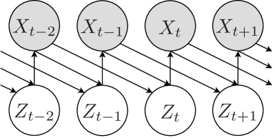
Figure 2: Variable dependences in a second-order KDE-MM. The generating component $Z$ is a latent variable.

Eq. (9) can be rewritten as

$$\widehat{f}_{X_{p+1}\;|\;\underline{X}_{1}^{p}}\left(x_{t}\;|\;\underline{x}_{t-p}^{t-1};\,h\right)\\ =\sum_{n=p+1}^{N}\kappa_{n}\left(\underline{x}_{t-p}^{t-1};\,h\right)\frac{1}{h}k\left(\frac{x_{t}-y_{n}}{h}\right)$$ (10)

$$\kappa_{n}\left(\underline{x}_{t-p}^{t-1};\,h\right)=\frac{\prod_{l=1}^{p}k\left(\frac{x_{t-l}-y_{n-l}}{h}\right)}{\sum_{n^{\prime}=p+1}^{N}\prod_{l=1}^{p}k\left(\frac{x_{t-l}-y_{n^{\prime}-l}}{h}\right)}\textrm{,}$$ (11)

which can be interpreted as a mixture model with context-dependent weights. To generate a new datapoint given the context $\underline{x}_{t-p}^{t-1}$, one selects a mixture component $Z_{t}\in\left\{p+1,\,\ldots,\,N\right\}$ according to the weights $\kappa_{n}\left(\underline{x}_{t-p}^{t-1};\,h\right)$. For KDE-MMs this component $z_{t}$ corresponds to an index into the database $\mathcal{D}$, identifying an exemplar $y_{z_{t}}$ upon which we base the sample at $t$. $x_{t}$ is then generated from $y_{z_{t}}$ with $k$-shaped noise added:

$$P\left(Z_{t}=n\;|\;\underline{X}_{t-p}^{t-1}=\underline{x}_{t-p}^{t-1};\,h\right) =\kappa_{n}\left(\underline{x}_{t-p}^{t-1};\,h\right)$$ (12)

$$\widehat{f}_{X_{p+1}\;|\;Z_{p+1},\,\underline{X}_{1}^{p}}\left(x_{t}\;|\;n,\,\underline{x}_{t-p}^{t-1};\,h\right) =$$ (13)

$$\widehat{f}_{X_{p+1}\;|\;Z_{p+1}}\left(x_{t}\;|\;n;\,h\right) =\frac{1}{h}k\left(\frac{x_{t}-y_{n}}{h}\right)\textrm{.}$$ (14)

This staggered structure is illustrated in Fig. 2 for a second-order model ($p=2$). The procedure is also simple to implement in software. It is easy to see that

$$\widehat{f}_{X_{p+1}\;|\;\underline{X}_{1}^{p}}\left(x_{p+1}\;|\;\underline{x}_{1}^{p}\right) \leq\max_{y_{n}\in\mathcal{D}}\frac{1}{h}k\left(\frac{x_{p+1}-y_{n}}{h}\right)\textrm{,}$$ (15)

regardless of context $\underline{x}_{1}^{p}$. This bounds the tails of $\widehat{f}_{X_{t}}$, so the $\widehat{X}$-process has as many finite moments as the kernel function does, ensuring stability.

The bandwidth $h$ affects the character of the generated data in two ways. With a sufficiently narrow bandwidth, and assuming $k$ has exponentially decreasing tails, the weight distribution $\kappa_{n}\left(\underline{x}_{t-p}^{t-1}\right)$ for $z_{t}$ will strongly favour the one $n$ that minimizes $\|\underline{x}_{t-p}^{t-1}-\underline{y}_{n-p}^{n-1}\|$; call this component $n^{\star}$. Since the added $k$-shaped noise in (14) has small variance, we have $x_{t}\approx y_{n^{\star}}$ in the typical case. This makes sampled sequences closely follow long segments of consecutive values from the training data series. If $h$ is increased, the weight distribution becomes more uniform, and sampled trajectories will increasingly often switch between different training-data segments, but the amount of added noise also grows. In Markov forecast densities and in KDE-HMMs as presented in the next section, the two roles of context sensitivity and additive noise level are assigned to separate parameters.

The idea of creating new samples by concatenating old data is reminiscent of the common block bootstrap for time series [32], albeit more refined, since the KDE-MM preferentially selects pieces that fit well together; this has advantages for the asymptotic convergence rate of bootstrap statistics [33]. Indeed, both [8] and [31] apply a bootstrap perspective when introducing KDE-based methods. The KDE-MM approach is also similar to waveform-similarity-based overlap-add techniques (WSOLA) [34] from signal processing, although these do not model probability distributions.

3.5 KDE Hidden Markov Models

Being Markov models, KDE-MMs capture short-range correlations in data series, but are not well-equipped to describe long-range memory or structure such as the sequential order of sounds in a speech utterance, as discussed in Section 2. To remedy this, we introduce a hidden (unobservable), discrete state variable $Q_{t}\in\left\{1,\,\ldots,\,M\right\}$ to the model in (9). $Q_{t}$ is governed by a first-order Markov chain. This results in hidden Markov models where the state-conditional output distributions are given by KDEs, specifically KDE-MMs. In other words, the current state $Q_{t}$ determines which of a set of $M$ KDE-MMs is used to generate the next sample value of the process. This construction is completely analogous to the setup of AR-HMMs [18], but with KDE-MMs instead of linear AR models. We call the new models kernel density hidden Markov models, or KDE-HMMs.

In this paper, we will work with models that, given the current state $Q_{t}=q$ and context $\underline{x}_{t-p}^{t-1}$, have the form

$$\widehat{f}_{X_{t}\;|\;Q_{t},\,\underline{X}_{t-p}^{t-1}}\left(x_{t}\;|\;q,\,\underline{x}_{t-p}^{t-1};\,\boldsymbol{K}\right)\\ =\sum_{n=p+1}^{N}\kappa_{qn}\left(\underline{x}_{t-p}^{t-1};\,\boldsymbol{K}\right)\frac{1}{h_{q0}}k_{q0}\left(\frac{x_{t}-y_{n}}{h_{q0}}\right)$$ (16)

$$\kappa_{qn}\left(\underline{x}_{t-p}^{t-1};\,\boldsymbol{K}\right) =\frac{w_{qn}\prod_{l=1}^{p}k_{ql}\left(\frac{x_{t-l}-y_{n-l}}{h_{ql}}\right)}{\sum_{n^{\prime}=p+1}^{N}w_{qn^{\prime}}\prod_{l=1}^{p}k_{ql}\left(\frac{x_{t-l}-y_{n^{\prime}-l}}{h_{ql}}\right)}\textrm{.}$$ (17)

$\boldsymbol{K}$ here denotes the set of KDE parameters, $\boldsymbol{K}=\left\{h_{ql},\,w_{qn}\right\}$ for $q\in\left\{1,\,\ldots,\,M\right\}$, $l\in\left\{0,\,\ldots,\,p\right\}$, and $n\in\left\{p+1,\,\ldots,\,N\right\}$. The function of the weights $w_{qn}$ is to allow the training data points to be assigned to different states. This assignment can be either hard (binary) or soft, but we require $w_{qn}\geq 0$ and $\sum_{n=p+1}^{N}w_{qn}=1$. We also allow kernel functions $k_{ql}$ and bandwidths $h_{ql}$ to depend on the state $q$ and lag $l$ considered. In addition to $\boldsymbol{K}$, we also have standard HMM parameters describing the hidden-state evolution, specifically a matrix $\boldsymbol{A}\in\mathbb{R}^{M\times M}$ of state transition probabilities defined by

$$a_{qq^{\prime}} =P\left(Q_{t+1}=q^{\prime}\;|\;Q_{t}=q\right)\textrm{.}$$ (18)

(Since the model is stationary and ergodic, the leading left eigenvector $\boldsymbol{\pi}\in\mathbb{R}^{M}$ of $\boldsymbol{A}$ satisfying $\sum_{q}\pi_{q}=1$ defines the stationary state distribution $P\left(Q_{t}=q\right)=\pi_{q}$ of the Markov chain. This also gives the initial state probabilities of the model.) The full set of KDE-HMM parameters is thus $\boldsymbol{\theta}=\left\{\boldsymbol{A},\,\boldsymbol{K}\right\}$. In Section 4 we derive update formulas to estimate these parameters from data.

To the best of our knowledge, models of the above form have not been considered previously. KDE-HMMs generalize [8] and [31] by introducing hidden states (when $M>1$) and different kernels and bandwidths for every lag $l$. Our proposal is also more general than HMMs with KDE outputs, dubbed KDE/HMM, previously investigated in [35]. We recover KDE/HMMs by setting $p=0$, making samples conditionally independent given the state sequence, similar to Fig. 1b.

Like with KDE-MMs, the next-step distribution of KDE-HMMs can be broken into two parts: one, $\kappa_{qn}$, choosing an exemplar $Z_{t}\in\left\{p+1,\,\ldots,\,N\right\}$ from $\mathcal{D}$ for the next step, given the context $\underline{x}_{t-p}^{t-1}$ and the current state $q_{t}$, and the other adding kernel-shaped noise around the selected exemplar value $y_{z_{t}}$. The dependences among variables in a KDE-HMM with $p=1$ are illustrated in Fig. 3. Despite the increased complexity, sampling is straightforward, and efficient inference remains possible for all $p$ using standard forward-backward recursions. Specifically, past and future values of $Q$ and $Z$ are conditionally independent given the sequence $\underline{x}$ and the state $q_{t}$ at time $t$, as can be verified, e.g., using the algorithm in [36].

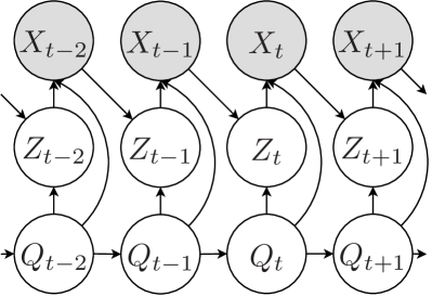
Figure 3: Variable dependences in a first-order KDE-HMM. The state $Q$ and component $Z$ are unobserved latent variables.

Adding a hidden state has several advantages. Aside from the benefits discussed in Sections 2.2 and 2.3, the state essentially partitions the space of contexts $\underline{x}_{t-p}^{t-1}$ into regions associated with different models, thus allowing different bandwidths for different situations. This can be a significant advantage in many cases—even when the data-generating process is Markovian—since it often is desirable to apply different degrees of smoothing in the modes versus the tails of distributions: see, for instance, [24] or [37], where the latter’s filtering functions $\rho_{j}\left(\cdot\right)$ closely resemble our weights $w_{qn}$. Letting the bandwidth depend on the lag $l$ furthermore allows better representation of phenomena such as variable (typically decreasing) predictive value of older samples, and separates context sensitivity ($h_{ql}$ for $l>0$) from the added noise ($h_{ql}$ for $l=0$) during sampling. This distinguishes KDE-HMMs from KDE-MMs even if the number of states, $M$, is one. As before, the advantages come at a price of greater demands for data and computation, compared to parametric approaches.

4 Parameter Estimation

To use models in practice, we must identify parameters that fit well for a given process of interest. In this section, we consider bandwidth selection and parameter estimation for KDE-MMs and KDE-HMMs. In particular, we derive guaranteed-ascent maximum likelihood update equations based on the EM-algorithm for the case of Gaussian kernels, along with relaxed update formulas which converge faster in practice.

4.1 Parameter Estimation Objective Function

Numerous principles have been proposed for choosing bandwidths in a data-driven manner (see [27] and [28] for reviews). In practice, the preferred scheme depends on the data and on the intended application, including the performance measure (loss function) of interest. In this paper we concentrate on the classic Kullback-Leibler (or KL) divergence from information theory,

$$D_{\mathrm{KL}}\left(f_{\boldsymbol{X}}\,\middle|\middle|\,\widehat{f}_{\boldsymbol{X}}\right) =\int f_{\boldsymbol{X}}\left(\boldsymbol{x}\right)\ln\frac{f_{\boldsymbol{X}}\left(\boldsymbol{x}\right)}{\widehat{f}_{\boldsymbol{X}}\left(\boldsymbol{x}\right)}\mathrm{d}\boldsymbol{x}\textrm{,}$$ (19)

previously used with KDE in signal processing and machine learning by [35] and [30]. Minimizing $D_{\mathrm{KL}}$ between empirical and estimated distributions leads to traditional maximum-likelihood (ML) parameter estimation, cf. [38]. While likelihood maximization is not considered appropriate for heavy-tailed reference densities $f_{\boldsymbol{X}}$ [39, 27], likelihoods are asymptotically a factor $N$ faster to evaluate compared to other bandwidth-selection criteria such as integrated squared error [30].

The likelihood function is given by Eqs. (9) and (16) applied to the training data sequence $\mathcal{D}=\underline{y}_{1}^{N}$, but it is not appropriate to optimize this function directly. In the limit where bandwidth goes to zero, the KDE $\widehat{f}_{\boldsymbol{X}}$ shrinks to a set of point masses (spikes) placed at the points in $\mathcal{D}$ and the likelihood diverges to positive infinity. A similar issue exists in common models such as Gaussian mixture models (GMMs) and Gaussian-output HMMs: by dedicating one component or state to a narrow spike centred on a single datapoint, arbitrarily high likelihood values can be achieved [1, pp. 433–434].

With KDE, a standard workaround is to use cross-validation, for every $t$ omitting the component centred at $y_{t}$ when computing the likelihood term at $\widehat{f}_{X}\left(y_{t};\,h\right)$. This prevents points in the training data from “explaining themselves” and removes the degenerate optimum at zero. The resulting objective function $\widetilde{f}$ is known as the pseudo-likelihood. It can be shown that, under certain conditions, maximizing the pseudo-likelihood asymptotically minimizes the KL-divergence of KDE [40].

For simplicity, we exclude the first $p$ points of all sequences, where the context is incomplete, from the KDE-HMM likelihood evaluations in this paper. (KDE-MMs use the periodic extension from footnote 4.) Using (17) and (16) then leads to the pseudo-likelihood

$$\widetilde{f}_{\underline{X}}\left(\underline{y}_{1}^{N};\,\boldsymbol{\theta}\right)=\sum_{\underline{q}_{p+1}^{N}}\sum_{\underline{z}_{p+1}^{N}}\widetilde{f}_{\underline{X},\,\underline{Q},\,\underline{Z}}\left(\underline{y}_{1}^{N},\,\underline{q}_{p+1}^{N},\,\underline{z}_{p+1}^{N};\,\boldsymbol{\theta}\right)$$ (20)

$$\widetilde{f}_{\underline{X},\,\underline{Q},\,\underline{Z}}\left(\underline{y}_{1}^{N},\,\underline{q}_{p+1}^{N},\,\underline{z}_{p+1}^{N};\,\boldsymbol{\theta}\right)=P\left(\underline{Q}_{p+1}^{N}=\underline{q}_{p+1}^{N};\,\boldsymbol{A}\right)\\ \cdot\prod_{t=p+1}^{N}\frac{\left(1-\delta_{z_{t}t}\right)w_{q_{t}z_{t}}\prod_{l=0}^{p}k_{q_{t}l}\left(\frac{y_{t-l}-y_{z_{t}-l}}{h_{q_{t}l}}\right)}{h_{q_{t}0}\sum_{n=p+1,\,n\neq t}^{N}w_{q_{t}n}\prod_{l=1}^{p}k_{q_{t}l}\left(\frac{y_{t-l}-y_{n-l}}{h_{q_{t}l}}\right)}\textrm{.}$$ (21)

The cross-validation terms $\left(1-\delta_{z_{t}t}\right)$ are introduced to set the probabilities of sequences having $z_{t}=t$ to zero.

To reduce clutter, we will from now on take the indices in expressions and summations to range as $q\in\left\{1,\,\ldots,\,M\right\}$, $l\in\left\{1,\,\ldots,\,p\right\}$, and $t,\,n\in\left\{p+1,\,\ldots,\,N\right\}$, unless otherwise specified. Primed indices follow the same limits as unprimed ones.

4.2 Expectation Maximization for KDE-HMMs

As with other latent-variable models such as GMMs and HMMs, direct analytic optimization of the (log) pseudo-likelihood is infeasible due to the sums over latent variables in (20). Instead, we seek an iterative optimization procedure based on the expectation maximization (EM) algorithm [41], by maximizing the auxiliary function

$$\mathcal{Q}\left(\boldsymbol{\theta}^{\prime};\,\widehat{\boldsymbol{\theta}}\right)\\ =\mathbb{E}\left(\ln\widetilde{f}_{\underline{X},\,\underline{Q},\,\underline{Z}}\left(\underline{y},\,\underline{Q},\,\underline{Z};\,\boldsymbol{\theta}^{\prime}\right)\;|\;\underline{X}=\underline{y};\,\widehat{\boldsymbol{\theta}}\right)\textrm{.}$$ (22)

Using Jensen’s inequality, one can prove that any revised parameter estimate $\widehat{\boldsymbol{\theta}}^{\left(\mathrm{new}\right)}$ satisfying

$$\mathcal{Q}\Big{(}\widehat{\boldsymbol{\theta}}^{\left(\mathrm{new}\right)};\,\widehat{\boldsymbol{\theta}}\Big{)} \geq\mathcal{Q}\left(\widehat{\boldsymbol{\theta}};\,\widehat{\boldsymbol{\theta}}\right)$$ (23)

is guaranteed not to decrease the actual likelihood of the data; this is used to establish convergence. In particular, convergence does not require maximizing (22) at every step, and procedures that increase $\mathcal{Q}$ without necessarily maximizing it are termed generalized EM (GEM). Because the pseudo-likelihood is equivalent to the regular likelihood together with a specific cross-validation prior on $Z$, convergence is assured also in our case.

At each EM iteration the shape of the auxiliary function is determined by the conditional posterior distribution of the latent variables $\underline{Q}$ and $\underline{Z}$. For KDE-HMMs, the relevant forward-backward recursions to determine the conditional hidden-state distributions, also known as state occupancies,

$$\gamma_{qt} =P\left(Q_{t}=q\;|\;\underline{X}_{1}^{N}=\underline{y}_{1}^{N};\,\widehat{\boldsymbol{\theta}}\right)$$ (24)

are identical to those of other HMMs with Markovian output distributions, such as [18], apart from enforcing $P\left(Z_{t}=t\right)=0\,\forall t$ due to cross-validation. The occupancies are used to update the state transition probabilities $\boldsymbol{A}$ of the KDE-HMM following standard HMM formulas available in [11].

Determining conditional posterior distributions, or responsibilities, of the latent KDE component variables $Z_{t}$ is similarly straightforward, and one obtains

$$\varrho_{qnt}^{\mathrm{num}} =P\left(Z_{t}=n\;|\;Q_{t}=q,\,\underline{X}_{t-p}^{t}=\underline{y}_{t-p}^{t};\,\widehat{\boldsymbol{K}}\right)$$ (25)

$$=\frac{\left(1-\delta_{nt}\right)\kappa_{qn}\left(\underline{y}_{t-p}^{t-1};\,\widehat{\boldsymbol{K}}\right)k_{q0}\left(\frac{y_{t}-y_{n}}{\widehat{h}_{q0}}\right)}{\sum_{n^{\prime}\neq t}\kappa_{qn^{\prime}}\left(\underline{y}_{t-p}^{t-1};\,\widehat{\boldsymbol{K}}\right)k_{q0}\left(\frac{y_{t}-y_{n^{\prime}}}{\widehat{h}_{q0}}\right)}\textrm{.}$$ (26)

The auxiliary function for weights and bandwidth parameters $\boldsymbol{K}$ then takes the form

$$\mathcal{Q}_{\boldsymbol{K}}\left(\boldsymbol{K}^{\prime};\,\widehat{\boldsymbol{K}}\right)=\sum_{q,\,t,\,n\neq t}\gamma_{qt}\varrho_{qnt}^{\mathrm{num}}\left(\ln w_{qn}^{\prime}-\frac{1}{2}\ln h_{q0}^{\prime}\right)\\ +\sum_{q,\,t,\,n\neq t}\gamma_{qt}\varrho_{qnt}^{\mathrm{num}}\sum_{l=0}^{p}\ln k_{ql}\left(\frac{y_{t-l}-y_{n-l}}{h_{ql}^{\prime}}\right)\\ -\sum_{q,\,t}\gamma_{qt}\ln\left(\sum_{n\neq t}w_{qn}^{\prime}\prod_{l}k_{ql}\left(\frac{y_{t-l}-y_{n-l}}{h_{ql}^{\prime}}\right)\right)\textrm{.}$$ (27)

Optimal values for the next-step bandwidths $h_{q0}^{\prime}$ are readily identified [35] and are presented in (28) below. The weights and context bandwidths ($w_{qn}^{\prime}$ and $h_{ql}^{\prime}$ for $l>0$) present an obstacle, however, as these appear in a negative term with a sum inside a logarithm and cannot be optimized analytically. Such terms are common in models that feature conditional probabilities with renormalization, e.g., standard maximum mutual information (MMI) discriminative classifiers [42].

To identify GEM updates of $\boldsymbol{K}$ with Gaussian kernels we construct a global lower bound $\underline{\mathcal{Q}}_{\boldsymbol{K}}$ of $\mathcal{Q}_{\boldsymbol{K}}$ in (27) which is tight at $\boldsymbol{K}^{\prime}=\widehat{\boldsymbol{K}}$. Any updated parameters $\boldsymbol{K}^{\prime}$ that does not decrease $\underline{\mathcal{Q}}_{\boldsymbol{K}}$ is then guaranteed not to decrease the true auxiliary function, and the key convergence relation (23) remains satisfied. This approach is known as minorize-maximization and can be seen as a generalization of EM [43].

While many bounds on log-sum-exp-type expressions exist [44], we chose to base our bound $\underline{\mathcal{Q}}_{\boldsymbol{K}}$ on so-called reverse-Jensen bounds [45, 46]. These apply to Gaussian and other exponential-family kernels that satisfy the conditions of Lemma 2, page 139 in [46]. Importantly, the reverse-Jensen bounds have the same parametric dependence on $\boldsymbol{K}^{\prime}$ as the other terms in Eq. (27), enabling us to to derive analytic expressions for the parameters $\widehat{\boldsymbol{K}}^{\left(\mathrm{new}\right)}$ that maximize the lower bound $\underline{\mathcal{Q}}_{\boldsymbol{K}}$.

A mathematically similar application of reverse-Jensen bounds to MMI training of HMM classifiers can be found in [47]. The resulting updates resemble those produced by a common MMI training technique called extended Baum-Welch (EBW) [48, 49]. However, while standard EBW equations include a heuristically set [50] tuning parameter that limits the update magnitude, the reverse-Jensen procedure selects the tuning parameter automatically, requiring no user intervention.

4.3 Generalized EM Update Formulas for KDE-HMM

For Gaussian kernels as in (4), maximizing the reverse-Jensen lower bound yields the GEM update equations

$$\widehat{h}_{q0}^{2\left(\mathrm{new}\right)} =\dfrac{\sum_{t,\,n\neq t}\gamma_{qt}\varrho_{qnt}^{\mathrm{num}}\left(y_{t}-y_{n}\right)^{2}}{\sum_{t,\,n\neq t}\gamma_{qt}\varrho_{qnt}^{\mathrm{num}}}$$ (28)

$$\widehat{h}_{ql}^{2\left(\mathrm{new}\right)} =\dfrac{W_{q}\widehat{h}_{ql}^{2}+\sum_{t,\,n\neq t}\gamma_{qnt}^{\mathrm{diff}}\left(y_{t-l}-y_{n-l}\right)^{2}}{W_{q}+\sum_{t,\,n\neq t}\gamma_{qnt}^{\mathrm{diff}}}$$ (29)

$$\widehat{w}_{qn}^{\left(\mathrm{new}\right)} =\frac{W_{q}\widehat{w}_{qn}+\sum_{t}\gamma_{qnt}^{\mathrm{diff}}}{W_{q}+\sum_{t,\,n^{\prime}\neq t}\gamma_{qn^{\prime}t}^{\mathrm{diff}}}$$ (30)

$$\gamma_{qnt}^{\mathrm{diff}} =\gamma_{qt}\left(\varrho_{qnt}^{\mathrm{num}}-\varrho_{qnt}^{\mathrm{den}}\right)$$ (31)

$$W_{q} =\sum_{t,\,n\neq t}\gamma_{qt}\left(\varrho_{qnt}^{\mathrm{den}}+\omega_{qnt}^{h}+\omega_{qnt}^{w}+\omega_{qnt}^{\prime}\right)\textrm{;}$$ (32)

the state occupancies $\gamma_{qt}$ in these formulas are defined by (24), while the responsibilities $\varrho_{qnt}^{\mathrm{num}}$ and the terms from the reverse-Jensen bound follow (26) and

$$\varrho_{qnt}^{\mathrm{den}} =P\left(Z_{t}=n\;|\;Q_{t}=q,\,\underline{X}_{t-p}^{t-1}=\underline{y}_{t-p}^{t-1};\,\widehat{\boldsymbol{K}}\right)$$ (33)

$$=\frac{\left(1-\delta_{nt}\right)\kappa_{qn}\left(\underline{y}_{t-p}^{t-1};\,\widehat{\boldsymbol{K}}\right)}{\sum_{n^{\prime}\neq t}\kappa_{qn^{\prime}}\left(\underline{y}_{t-p}^{t-1};\,\widehat{\boldsymbol{K}}\right)}$$ (34)

$$\omega_{qnt}^{h} =2G\left(\frac{1}{2}\varrho_{qnt}^{\mathrm{den}}\right)\sum_{l=1}^{p}\left(\xi_{ql}^{h}\right)^{2}$$ (35)

$$\omega_{qnt}^{w} =4G\left(\frac{1}{2}\varrho_{qnt}^{\mathrm{den}}\right)\xi_{qn}^{w}$$ (36)

$$\omega_{qnt}^{\prime} =\varrho_{qnt}^{\mathrm{den}}\max\left(\max_{l}\left(\xi_{ql}^{h}\right),\,\xi_{qn}^{w}\right)$$ (37)

$$\xi_{ql}^{h} =\left(y_{t-l}-y_{n-l}\right)^{2}\widehat{h}_{ql}^{-2}-1$$ (38)

$$\xi_{qn}^{w} =\widehat{w}_{qn}^{-1}-1\textrm{.}$$ (39)

The function

$$G\left(\gamma\right) =\begin{cases}\left(\frac{\gamma-1}{\ln\gamma}\right)^{2}-\frac{1}{4\ln\gamma}&\textrm{if }\gamma<\nicefrac{{1}}{{6}}\\ \left(\frac{\nicefrac{{1}}{{6}}-1}{\ln\nicefrac{{1}}{{6}}}\right)^{2}-\frac{1}{4\ln\nicefrac{{1}}{{6}}}+\gamma-\frac{1}{6}&\textrm{otherwise}\end{cases}$$ (40)

follows Eq. (5.10) in [46, p. 99].

The update formulas in (28) through (30) should increase the pseudo-likelihood except at local extreme points. Since

$$W_{q}+\sum_{t,\,n\neq t}\gamma_{qnt}^{\mathrm{diff}} >0\textrm{,}$$ (41)

the updated parameters are always well defined.

Prop. 1.

Let $\widehat{\boldsymbol{\theta}}^{\left(i\right)}$ for $i\in\mathbb{Z}_{+}$ be a sequence of parameter estimates, computed iteratively from $\mathcal{D}=\underline{y}_{1}^{N}$ using the update procedure above, and let $\widetilde{f}^{\left(i\right)}$ be the corresponding pseudo-likelihoods in Eq. (20). Define the minimum separation $d_{\mathrm{min}}$ through

$$d_{\mathrm{min}} =\min_{t,\,n\neq t}\left|y_{t}-y_{n}\right|\textrm{.}$$ (42)

Assume $d_{\mathrm{min}}$ is strictly positive and $N>p+1$. Then $\lim_{i\to\infty}\widetilde{f}^{\left(i\right)}$ exists.

The proof proceeds by establishing that the pseudo-likelihood has a finite upper bound $\widetilde{f}_{\mathrm{max}}$, and then showing that $\widetilde{f}_{\mathrm{max}}\geq\widetilde{f}^{\left(i+1\right)}\geq\widetilde{f}^{\left(i\right)}\,\forall i$, which ensures convergence.

4.4 Accelerated Updates

Studying the update equations, we see that the quantity $W_{q}$ limits the update step length: if $W_{q}$ is large compared to $\left|\sum_{t,\,n\neq t}\gamma_{qnt}^{\mathrm{diff}}\right|$, we have $\widehat{h}_{ql}^{\left(\mathrm{new}\right)}\approx\widehat{h}_{ql}$, and similarly for $\widehat{w}_{qn}^{\left(\mathrm{new}\right)}$. Unfortunately, $W_{q}$ often substantially exceeds $\left|\sum_{t,\,n\neq t}\gamma_{qnt}^{\mathrm{diff}}\right|$ on large datasets, and the time required until eventual convergence is then infeasibly long.

To reduce $W_{q}$ and obtain formulas that produce larger updates, one may let the weights $w_{qn}$ be fixed (as their updates drive up the $W_{q}$-factors the most) and only consider updating the bandwidths. We can then set $\xi_{qn}^{w}=0$ in all formulas. Moreover, we apply the approximation $G\left(\gamma\right)\approx\gamma$, which is the first of several steps involved in connecting reverse-Jensen update formulas to standard EBW heuristics [47]. This yields the approximate weights

$$\widetilde{\omega}_{qnt}^{h} =\varrho_{qnt}^{\mathrm{den}}\sum_{l}\left(\xi_{ql}^{h}\right)^{2}\textrm{,}$$ (43)

and the associated relaxed $W_{q}$-factors

$$\widetilde{W}_{q} =\sum_{t,\,n\neq t}\gamma_{qt}\left(\varrho_{qnt}^{\mathrm{den}}+\widetilde{\omega}_{qnt}^{h}+\omega_{qnt}^{\prime}\right)\textrm{.}$$ (44)

(It is important to remember that $\omega_{qnt}^{\prime}$ here should use $\xi_{qn}^{w}=0$.) The resulting KDE-HMM training algorithm is summarized in Table I.

Table I: Accelerated training of Guassian-kernel KDE-HMMs.

function TrainKDE-HMM($\underline{y}_{1}^{N},\,\widehat{\boldsymbol{A}},\,w_{qn},\,\widehat{h}_{q0},\,\widehat{h}_{ql}$)

    $\xi_{qn}^{w}\leftarrow 0$

    compute initial state distribution $\widehat{\boldsymbol{\pi}}$ from $\widehat{\boldsymbol{A}}$

    repeat

        compute $\widehat{\alpha}_{qt},\,\widehat{\beta}_{qt},\,\gamma_{qt}$ using forward-backward [11]

        re-estimate $\widehat{\boldsymbol{A}}$ using standard formula [11]

        recompute $\widehat{\boldsymbol{\pi}}$ from $\widehat{\boldsymbol{A}}$

        compute $\varrho_{nt}^{\mathrm{num}},\,\varrho_{nt}^{\mathrm{den}}$ using (26), (34)

        compute $\gamma_{qnt}^{\mathrm{diff}}$ using (31)

        compute $\xi_{ql}^{h}$ using (38)

        compute $\widetilde{\omega}_{qnt}^{h},\,\omega_{qnt}^{\prime}$ using (43), (37)

        compute $\widetilde{W}_{q}$ using (44)

        re-estimate $\widehat{h}_{q0},\,\widehat{h}_{ql}$ using (28), (29)

    until convergence

    return $\widehat{\boldsymbol{A}},\,w_{qn},\,\widehat{h}_{q0},\,\widehat{h}_{ql}$

end function

Since $\widetilde{W}_{q}$ in (44) tends to be of roughly the same order of magnitude as $\left|\sum_{t,\,n\neq t}\gamma_{qnt}^{\mathrm{diff}}\right|$, EM-training with $\widetilde{W}_{q}$ instead of $W_{q}$ converges quite quickly. On the other hand, $\widetilde{W}_{q}$ remains sufficiently conservative to virtually always increase the likelihood at every step in our experiments.

4.5 KDE-MM Bandwidth Selection

We now turn to consider the special case of KDE-MMs. While bandwidth selection formulas for KDE-MM-like models do exist in the literature, e.g., [51], these focus on mean squared error rather than pseudo-likelihood. Since KDE-MMs essentially are single-state KDE-HMMs with fixed, uniform weights $w_{1n}=\frac{1}{N}$ and all bandwidths tied to be equal, the approach in this paper can also be used to derive pseudo-likelihood maximization formulas for the KDE-MM bandwidth $h$. Assuming a Gaussian kernel this yields the iterative updates

$$\widehat{h}^{2\left(\mathrm{new}\right)} =\dfrac{W\widehat{h}^{2}+\sum_{t,\,n\neq t}\left(\varrho_{nt}^{\mathrm{num}}\left(y_{t}-y_{n}\right)^{2}+p\varrho_{nt}^{\mathrm{diff}}\overline{d}_{nt}^{2}\right)}{W+\sum_{t,\,n\neq t}\left(\varrho_{nt}^{\mathrm{num}}+p\varrho_{nt}^{\mathrm{diff}}\right)}$$ (45)

$$\varrho_{nt}^{\mathrm{diff}} =\varrho_{nt}^{\mathrm{num}}-\varrho_{nt}^{\mathrm{den}}$$ (46)

$$W =p\sum_{t,\,n\neq t}\left(\varrho_{nt}^{\mathrm{den}}+\omega_{nt}+\omega_{nt}^{\prime}\right)$$ (47)

$$\omega_{nt} =2pG\left(\frac{1}{2}\varrho_{nt}^{\mathrm{den}}\right)\left(\overline{d}_{nt}^{2}\widehat{h}^{-2}-1\right)^{2}$$ (48)

$$\omega_{nt}^{\prime} =\varrho_{nt}^{\mathrm{den}}\max\left(\overline{d}_{nt}^{2}\widehat{h}^{-2}-1,\,0\right)$$ (49)

$$\overline{d}_{nt}^{2} =\frac{1}{p}\sum_{l}\left(y_{t-l}-y_{n-l}\right)^{2}\textrm{.}$$ (50)

with $\varrho_{nt}^{\mathrm{num}}$ and $\varrho_{nt}^{\mathrm{den}}$ defined as in Eqs. (26) and (34), respectively, but with all references to the state $q$ omitted. Just as for KDE-HMMs, the approximation $G\left(\gamma\right)\approx\gamma$ can be introduced to obtain relaxed weights

$$\widetilde{W} =p\sum_{t,\,n\neq t}\left(\varrho_{nt}^{\mathrm{den}}+\widetilde{\omega}_{nt}+\omega_{nt}^{\prime}\right)$$ (51)

$$\widetilde{\omega}_{nt} =p\varrho_{nt}^{\mathrm{den}}\left(\overline{d}_{nt}^{2}\widehat{h}^{-2}-1\right)^{2}$$ (52)

which increase the stepsize of the updates. Alternatively, it is straightforward to maximize the pseudo-likelihood using general-purpose numerical optimization methods, as KDE-MMs only have a single free parameter.

4.6 Initialization

Similar to traditional training schemes for HMMs, the proposed parameter estimation schemes for KDE-MMs and KDE-HMMs rely on iterative refinements, and thus require initialization. For standard EM-training of models such as HMMs and AR-HMMs, it is sufficient to provide an initial guess $\widehat{\gamma}_{qt}$ of the state occupancies given $\underline{y}_{1}^{N}$ to begin estimating parameters. In contrast, our KDE-HMM update formulas, like EBW, depend on previous parameter values. Initial weights and bandwidth parameters must therefore be assigned explicitly. We propose to set the weight parameters based on state occupancies according to

$$\widehat{w}_{qn} =\frac{\widehat{\gamma}_{qn}}{\sum_{n^{\prime}}\widehat{\gamma}_{qn^{\prime}}}\textrm{,}$$ (53)

as an estimate of the conditional component probabilities $P\left(Z_{t}=n\;|\;Q_{t}=q;\,\boldsymbol{\theta}\right)$. Initial bandwidths $\widehat{h}_{q0}$ and $\widehat{h}_{ql}$ can then be set using the multidimensional KDE “normal reference rule” from [52, 53], with each point weighted according to $w_{qn}$, while the transition matrix may be initialized based on co-occurrences,

$$\widehat{a}_{qq^{\prime}} =\frac{\sum_{t=1}^{N-1}\widehat{\gamma}_{qt}\widehat{\gamma}_{q^{\prime}\left(t+1\right)}}{\sum_{t=1}^{N-1}\widehat{\gamma}_{qt}}\textrm{.}$$ (54)

Sometimes occupancy estimates $\widehat{\gamma}_{qn}$ for seeding the model can be computed based on domain knowledge or by inspecting the data. This approach will be used for the experiments in this article. Another common principle is to base advanced models on faster, simpler methods, e.g., using $k$-means to initialize GMMs. For KDE-HMMs it is natural to set $\widehat{\gamma}_{qn}=\gamma_{qn}^{\left(\mathrm{HMM}\right)}$, where $\gamma_{qn}^{\left(\mathrm{HMM}\right)}$ are the state occupancies of a trained parametric hidden-state model such as an HMM or an AR-HMM.

The mechanics of KDE-HMM initialization are summarized in Table II. Given a trained model, the probability of any given observation sequence under $\boldsymbol{\theta}$ can be evaluated with the forward algorithm, just like for regular HMMs [11]. Sequentially generating samples from the model is similarly straightforward.

Table II: Initialization of Gaussian-kernel KDE-HMMs.

function GammasToKDE-HMM($\underline{y}_{1}^{N},\,\widehat{\gamma}_{qt}$)

    compute $\widehat{\boldsymbol{A}}$ using (54)

    compute $\widehat{w}_{qn}$ using (53)

    compute $\widehat{h}_{q0},\,\widehat{h}_{ql}$ using weighted reference rule [52, 53]

    return $\widehat{\boldsymbol{A}},\,\widehat{w}_{qn},\,\widehat{h}_{q0},\,\widehat{h}_{ql}$

end function

function HMMToKDE-HMM($\underline{y}_{1}^{N}$, an HMM $\boldsymbol{\lambda}$)

    compute $\widehat{\gamma}_{qt}$ from $\boldsymbol{\lambda}$ using forward-backward [11]

    take $\widehat{\boldsymbol{A}}$ from $\boldsymbol{\lambda}$

    compute $\widehat{w}_{qn}$ using (53)

    compute $\widehat{h}_{q0},\,\widehat{h}_{ql}$ using weighted reference rule [52, 53]

    return $\widehat{\boldsymbol{A}},\,\widehat{w}_{qn},\,\widehat{h}_{q0},\,\widehat{h}_{ql}$

end function

5 Experiments on Synthetic Data

To investigate the probabilistic modelling capabilities of KDE-MMs and KDE-HMMs, we applied these techniques to a selection of datasets, and compared their prediction performance against other, standard time-series models representing the different time-dependence paradigms discussed in Section 2.

In this section, we consider an application to synthetic data, illustrating the strong, general asymptotic convergence properties of KDE-based models, also for non-Gaussian processes that baseline predictors cannot describe. Applications to nonlinear real-life datasets are considered in Section 6.

5.1 Data Series

As a first test, we generated data from a simple reference process having both hidden-state and Markovian dependences as in Fig. 1c. Specifically, we used a first-order linear AR-HMM with two states as the data source. We let both state-conditional AR-processes have the same mean (zero) and correlation coefficient $\nicefrac{{2}}{{3}}$, but gave one state a much larger standard deviation for the driving noise ($\sigma_{1}=1$ versus $\sigma_{2}=5$). We can write this process as

$$X_{t} =\frac{2}{3}X_{t-1}+\sigma_{Q_{t}}U_{t}\textrm{,}$$ (55)

where $U_{t}$ is zero-mean, unit-variance white noise. A symmetric hidden-state transition matrix $\boldsymbol{A}$ was chosen, with a probability $a_{qq}=\nicefrac{{4}}{{5}}$ of staying in the same state, and $1-a_{qq}=\nicefrac{{1}}{{5}}$ of switching to the other state at each time step. This produced time series cycling through volatile and quiescent periods, similar to stock market data.

We considered two variations of the above model, differing in the properties of the driving noise $U_{t}$. In the first application, we let $U_{t}$ be i.i.d. standard normal distributed, while in the second, we used independent samples from the bimodal zero-mean Gaussian mixture

$$f_{U_{t}}\left(u\right)=\frac{1}{\sqrt{2\pi}\sigma_{U}}\sum_{c=0}^{1}\exp\left(-\frac{1}{2}\left(\frac{u-\left(-1\right)^{c}\mu_{U}}{\sigma_{U}}\right)^{2}\right)$$ (56)

$$\mu_{U}=\sqrt{\frac{36}{37}}\textrm{,}\qquad\sigma_{U}=\frac{1}{\sqrt{37}}\textrm{,}$$ (57)

which also has unit variance.

For each of the two data sources above, five different training data sizes $N$ between $N=10^{1.5}$ and $N=10^{3.5}$ were considered. For each data size, 30 independent realizations were generated of each process, along with 30 independent validation sets of $T=1000$ samples.

5.2 Experiment Setup

We applied five different models to the datasets to investigate model convergence speed and asymptotic prediction performance as a function of training data size. The tested models were a first-order linear Gaussian autoregressive model; a two-state Gaussian-output HMM; a two-state, first-order Gaussian AR-HMM (combining the first two models); a first-order KDE-MM trained by numerically optimizing the pseudo-likelihood; and a two-state, first-order KDE-HMM trained using the algorithm in Table I. The models are summarized in Table III.

All hidden-state models in this paper, KDE-HMMs included, were initialized based on estimated state occupancies $\widehat{\gamma}_{qn}$ as outlined in Section 4.6. Because of the cyclic nature of the data series considered, we found it natural to compute $\widehat{\gamma}_{qn}$ based on estimates of the progression through these cycles, i.e., by quantizing simple estimates of the instantaneous phase. To be as fair as possible, the same initial occupancy values were used across all hidden-state models in a given experiment.

Table III: Comparison of models used in the experiments. Hidden-state models used $M\leq 15$ states, with $M=1$ equivalent to no hidden state. Explicit Markovian dependences were of order $p\leq 10$, with $p=0$ equivalent to no explicit Markovian dependence between observations.

Model	Time dependence		Added
type	Hidden state	Markov	noise
AR	no	linear AR	Gaussian
HMM	yes	no	Gaussian
AR-HMM	yes	linear AR	Gaussian
KDE-MM	no	KCDE, 1 bandwidth
KDE-HMM	yes	KCDE, $M\left(p+1\right)$ bandwidths

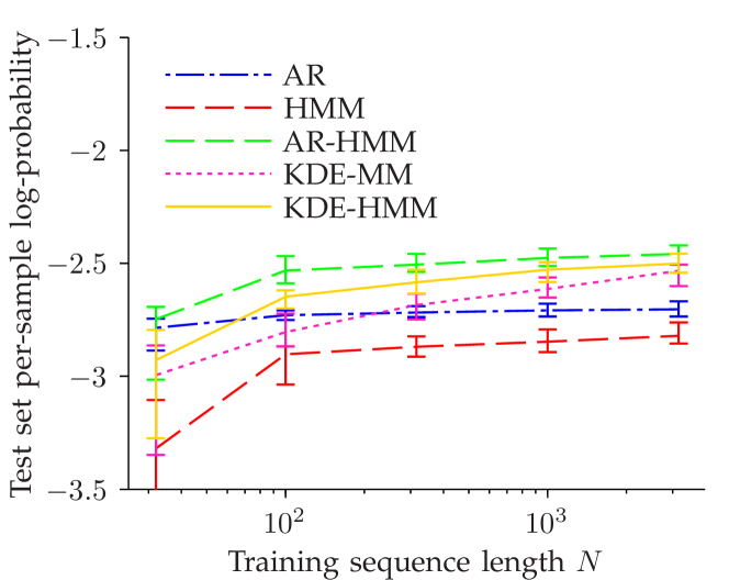
(a) Gaussian-noise driven AR-HMM data.

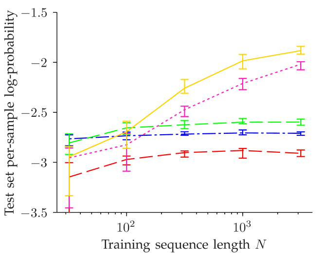
(b) GMM-driven AR-HMM data.

Figure 4: Median held-out set performance of parametric and nonparametric models from different paradigms as a function of training dataset size, with error bars at 25% and 75% quantiles. The data was generated by a simple two-state, first-order AR-HMM, but the two figures differ in the nature of the underlying driving noise.

For the heteroscedastic data considered in this first experiment, the state (discrete phase) of the variance cycle was estimated based on the magnitude of process value changes. We then assigned datapoints to low or high-volatility states using the simple thresholding scheme

$$\widehat{\gamma}_{1n}= \begin{cases}1&\textrm{if }n>1\textrm{ and }\left|y_{n}-y_{n-1}\right|\leq\Delta_{\mathrm{th}}\\ \nicefrac{{1}}{{2}}&\textrm{if }n=1\textrm{ (since $y_{0}$\ is undefinded)}\\ 0&\textrm{otherwise}\end{cases}$$ (58)

and $\widehat{\gamma}_{2n}=1-\widehat{\gamma}_{1n}$, where

$$\Delta_{\mathrm{th}} =\mathrm{median}\,\left\{\left|y_{n}-y_{n-1}\right|\right\}_{n=2}^{N}\textrm{.}$$ (59)

Similar to KDE-HMMs, the single KDE-MM bandwidth parameter was initialized based on the normal reference rule [52, 53].

For each dataset generated, each of the five models we consider was initialized and subjected to 500 iterations on the training data (excluding linear AR models which do not require iteration). The trained models were then asked to compute the log-probability of the corresponding set of separate but similarly generated validation data. Figs. 4a and 4b illustrate the median validation set performance for different training data sizes $N$ on the two data sources, with one curve for each method, surrounded by 25% and 75% quantile intervals. Higher log-probabilities are better; an upper bound on expected performance is given by the differential entropy rate of the data source.

5.3 Analysis

Despite the simplistic choice of weights $w_{qn}$, KDE-HMMs were capable of learning good models of autoregressive hidden-state processes driven both by Gaussian noise as well as by more general GMM noise, given a sufficient amount of data. On the other hand, neither pure Markovian nor pure hidden-state models were a good fit for GMM-driven data, though the models are likely to improve in asymptotic performance if more states or higher orders were to be considered.

Unsurprisingly, parametric models converged faster than KDE-HMMs, but provided inferior asymptotic performance unless the data was generated by a model within their particular parametric class. This is why Gaussian AR-HMMs show good performance in the first figure, where $U_{t}$ happens to be Gaussian, but not in the second, where $U_{t}$ follows a GMM. In fact, all non-KDE models show reduced asymptotic performance for the second dataset, even though the underlying process has lower entropy rate, making it, in principle, easier to predict. The issue is that the parametric models place the majority of their probability mass in regions near the next-step conditional mean $\mathbb{E}\left(X_{t+1}\;|\;\underline{x}_{1}^{t}\right)$, where the true pdf is quite small.

6 Experiments on Real-Life Data

In our second set of experiments, we investigated the capabilities of KDE-MMs and KDE-HMMs for describing several challenging natural processes of interest in nonlinear prediction, and compared against baseline models. The results affirmed the advantages of KDE-based techniques. Moreover, the lag-dependent bandwidths and hidden-state memory of KDE-HMMs were shown to improve on KDE-MM performance for all datasets.

6.1 Data Series

For our first real-world application, we considered the laser data (dataset A and its continuation) from the Santa Fe time-series prediction contest described in [54]. This data was also used in [55] and [5], for instance. The data consists of integer-quantized intensity measurements from a laser in a chaotic state. To avoid issues with degenerate likelihoods due to coinciding points (a problem with all latent-variable models considered) uniform noise over $\left(-\nicefrac{{1}}{{2}},\,\nicefrac{{1}}{{2}}\right)$ was added to the data.

A plot of the first 300 points of the laser data is provided in Fig. 5a. The series shows oscillations, about seven samples long, that slowly increase in magnitude, only to eventually fizzle out and start over again.

The second data series consisted of raw AD-converter values from an ECG signal sampled at 128 Hz, specifically series 16265 in the MIT-BIH Normal Sinus Rhythm Database from PhysioNet [56]. This data was previously considered in [57]. Like the laser data, uniform noise was added to counteract quantization effects. A plot of the first 300 points of the data is provided in Fig. 5b. The data has the characteristic ECG shape, showing regular, distinct pulses with lesser activity in between.

For both datasets, the first $N=3000$ points were used for training and the $N$ subsequent points for validation.

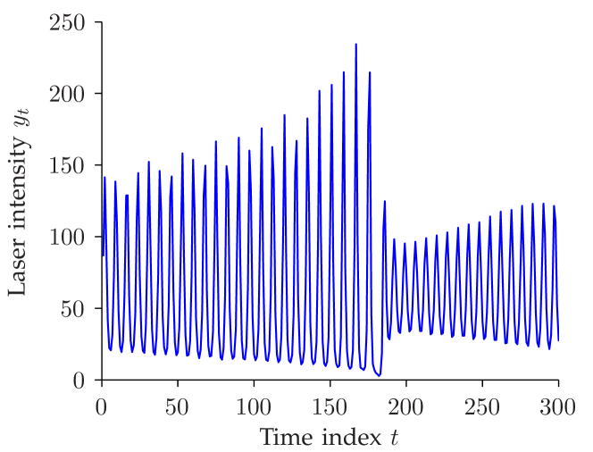
(a) Excerpt from laser data.

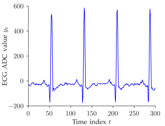
(b) Excerpt from ECG data.

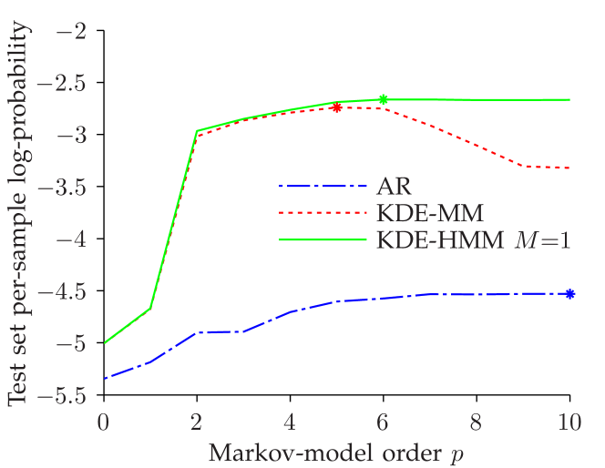
(c) Markov-model performance on laser data.

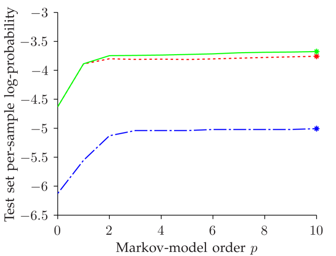
(d) Markov-model performance on ECG data.

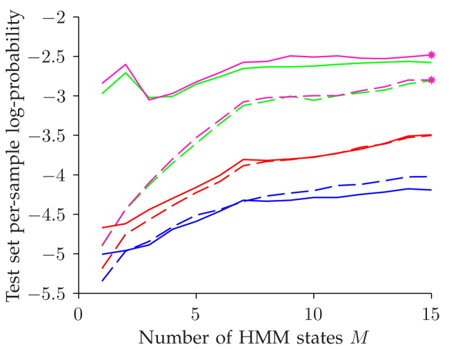
(e) Hidden Markov model performance on laser data.

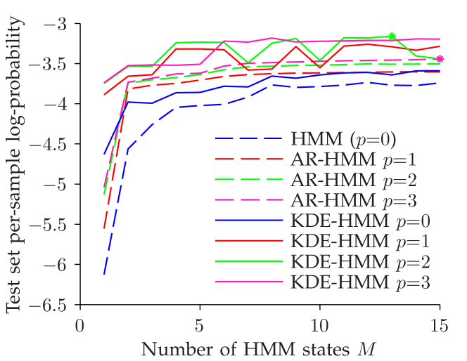
(f) Hidden Markov model performance on ECG data.

Figure 5: Training series and held-out set (natural) log-probability of various models for real-life data experiments. Standard AR models are dash-dotted, HMMs and AR-HMMs are dashed, KDE-MMs are dotted, and KDE-HMMs are drawn solid. Asterisks mark the best model of each kind. In the last two figures, colours reflect model order $p$.

6.2 Markov-Model Experiment

A number of experiments were performed on each dataset. In a first application, three different types of Markov models were compared. Specifically, linear AR-models, KDE-MMs, and KDE-HMMs with a single state (so no long-range memory) of orders $p=0$ (corresponding to a conditional independence assumption) through $10$ were fitted to the training data. The models were initialized as in Section 4.6, but with $\gamma_{1t}=1$ since only a single state was used. Due to the low dimensionality of the parameter space, Matlab fminunc sufficed for optimizing KDE bandwidths.

After training, the models were asked to assess the probability of the held-out validation data, with results as shown in Figs. 5c and 5d. Higher probabilities are preferred, as before. Apart from stochastic effects, increased held-out set log-probability directly implies a proportional reduction in KL-divergence, cf. (19).

The results of the Markov-model experiment highlight the power of nonparametric approaches for nonlinear datasets. KDE-MMs greatly outperform linear AR models of the same order. Single-state ($M=1$) KDE-HMMs, which additionally offer lag-dependent bandwidths, are better still, showing minor improvements over KDE-MMs everywhere except at $p=0$, where the two models coincide. Since the nonparametric models use the information provided by the context more efficiently, their performance saturates faster, and at a higher level, as $p$ increases.

The fact that general nonparametric density estimation rapidly becomes more data-demanding in higher dimensions [24] could be cause for concern, as our models conceptually are based on estimating $f_{\underline{X}_{1}^{p+1}}$ using KDE. However, the experiments show that high dimensionalities are not as problematic as may have been anticipated, and KDE-HMMs consistently work well all the way up to $p+1=11$-dimensional contexts. One explanation is that KDE-HMMs are capable of automatic relevance determination: by setting $h_{ql}$ large, the corresponding context values $y_{n-l}$ exert negligible influence on the distribution of $y_{n}$. Models can thus ignore non-informative lags. (Linear AR-models have similar abilities to exclude variables from consideration.) The learned laser data bandwidth parameters were found to be very wide for $l>6$, consistent with this hypothesis. KDE-MMs, in contrast, are constrained to use the same bandwidths for all lags and may suffer when the context includes variables of little predictive value, explaining the performance roll-off after $p=6$ in Fig. 5c.

6.3 Hidden Markov Model Experiment

Next, we investigated the benefits of adding a hidden state to the various models. To do this, we trained both KDE-HMMs and regular HMMs with Gaussian autoregressive outputs (AR-HMMs [18]) of orders $p=0$ through $3$, with $M$ states, $M\in\left\{1,\,\ldots,\,15\right\}$, for each $p$. When $p=0$, the AR-HMMs reduce to ordinary HMMs with Gaussian output distributions, while the KDE-HMMs resemble the KDE/HMMs in [35]. Many Markov models in the previous section are special cases for $M=1$.

All the participating models were initialized using the same scheme as in the previous experiments. Like in Section 5.2, initial state occupancies $\widehat{\gamma}_{qt}$ were based on the estimated cycle state. To estimate the continuous instantaneous phase for initialization, the peak of each oscillation cycle in the data was extracted; by assuming consecutive peaks were separated by a phase difference of $2\pi$, instantaneous phase values $\widehat{\varphi}_{t}$ for all $t$ could be interpolated using cubic splines. The initial occupancies were computed as a soft quantization of this phase,

$$\widehat{\gamma}_{qt} =\max\left(0,\,1-\frac{M}{2\pi}\min\left(\Delta\widehat{\varphi}_{qt},\,2\pi-\Delta\widehat{\varphi}_{qt}\right)\right)$$ (60)

$$\Delta\widehat{\varphi}_{qt} =\left(\widehat{\varphi}_{t}-2\pi\frac{q-1}{M}\right)\mathrm{mod}\,2\pi\textrm{.}$$ (61)

This satisfies $\sum_{q}\widehat{\gamma}_{qt}=1$ for all $t$, as required, and provides a sparse initialization where most $\widehat{\gamma}_{qt}$-values are zero. The setup promotes a hidden-state memory that tracks the current position in the cycle, for instance biasing ECG pulses to appear at regular intervals.

Following training, the log-probability of the held-out dataset was computed under each model, with results as in Figs. 5e and 5f. A number of trends are evident in these figures. First, combining the local continuity of Markov models with the hidden state variable of HMMs as suggested in 2.3 increased the accuracy of both the parametric and the nonparametric techniques. For a fixed $p$, increasing $M$ typically improved performance across all models. This is especially clear when going from $M=1$ to $M=2$, but we also note that hidden-state model performance at high $M$ exceeds the asymptotic levels attained by the Markov-models in Figs. 5c and 5d, even though these used considerably higher $p$-values. Conversely, given a fixed $M$, increasing $p$ often proved beneficial, particularly at low orders. In other words, more parameters tended to help, both for the linear, parametric baseline models and for KDE-HMMs.

Most importantly, even though the weaker linear AR models obviously had the most to gain from adding a hidden state, the figures show that KDE-HMMs provided greater accuracy than parametric models of similar order $p$ and state-set size $M$. This is true for all graphs in Fig. 5f, and for the laser results in 5e once $p\geq 2$.

For the ECG data in 5f, KDE-HMM behaviour at $p\geq 1$ appears somewhat inconsistent, in that performance seems to fluctuate between two distinct levels, one noticeably better than the other. This suggests that the maximization procedure, being sensitive to initialization, sometimes converged to local optima of inferior quality. Despite the fluctuations, KDE-HMMs always outperform their matching AR-HMM counterparts for all $\left(M,\,p\right)$ combinations in the figure.

As discussed in Section 2.2, the addition of a hidden state helps both by partitioning the context-space and by providing long-range memory. The results show that such partitioning is useful for all model types, but especially benefits weaker models like Gaussian, linear AR, by enabling a crude form of nonlinearity where different parts of the data are described by different models. KDE-HMMs further improve on parametric hidden-state approaches by relaxing assumptions on distributions and within-state linearity.

Data partitioning also gives KDE-HMMs an edge over KDE-MMs, since it allows for context-dependent bandwidths. This is illustrated by Fig. 6, displaying a scatter plot of the laser training data, with each datapoint coloured by state assignment ($\widehat{q}_{n}=\mathrm{argmax}_{q}\gamma_{qn}$) for the best-performing KDE-HMM ($M=15$, $p=3$). Drawing each point as an ellipse centred on $\left(y_{n-1},\,y_{n}\right)$ with axes dimensioned according to $\widehat{h}_{\widehat{q}_{n}l}$, we can confirm that the trained model adaptively uses wider bandwidths in regions where data is sparse, but employs narrower bandwidths to bring out detail in more concentrated regions. A KDE-MM, in contrast, cannot do this, and is forced to use a wide compromise bandwidth throughout.

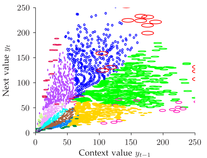
Figure 6: Scatter plot illustrating state-dependent kernel widths $\widehat{h}_{\widehat{q}_{n}l}$ of KDE-HMM trained on the laser data. Colours are based on datapoint state assignment $\widehat{q}_{n}=\mathrm{argmax}_{q}\gamma_{qn}$. The swirly pattern of the data is due to structure in the strange attractor.

As anticipated, parametric models were faster to work with throughout the experiments, since their computational demands per training iteration are linear in $N$, whereas KDEs with pseudo-likelihood maximization scale as $\mathcal{O}\left(N^{2}\right)$. We envision that additional approximations, particularly in the style of [30], will be essential to fast computation in large-scale applications. We also expect KDE-HMM accuracy would improve further, and the top-left dip in the performance curves in Fig. 5e could be eliminated, if the weights $w_{qn}$ could be trained efficiently.

7 Conclusions and Future Work

We have described KDE-MMs and KDE-HMMs as nonlinear, nonparametric models of stochastic time series. Unlike traditional parametric approaches, these models can represent a broad class of continuous-valued stochastic processes, including all Markov processes. We also detailed how the models can be trained, and demonstrated good modelling performance in applications to synthetic and natural data.

For future applications it is especially compelling to investigate the use of KDE-HMMs in speech synthesis. The KDE-HMM data-generation mechanism, which in essence concatenates datapoints from the training material in a context-sensitive manner, is evocative of concatenative speech synthesis as popularized by [58], except that KDE-HMMs also are fully probabilistic. This is promising, seeing that synthesis techniques based on probabilistically-guided exemplar concatenation have produced leading results in recent speech-synthesis challenges [59, 60].

References

- [1] C. M. Bishop, Pattern Recognition and Machine Learning. New York, NY: Springer, 2006.
- [2] G. E. Henter, “Probabilistic sequence models with speech and language applications,” Ph.D. dissertation, KTH – Royal Inst. Technol., Stockholm, Sweden, 2013. [Online]. Available: http://urn.kb.se/resolve?urn=urn:nbn:se:kth:diva-134693
- [3] H. Tong and K. S. Lim, “Threshold autoregression, limit cycles and cyclical data,” J. Roy. Stat. Soc. B, vol. 42, no. 3, pp. 245–292, 1980.
- [4] A. Waibel, T. Hanazawa, G. Hinton, K. Shikano, and K. J. Lang, “Phoneme recognition using time-delay neural networks,” IEEE T. Acoust. Speech, vol. 37, no. 3, pp. 328–339, 1989.
- [5] M. Kallas, P. Honeine, C. Richard, C. Francis, and H. Amoud, “Kernel-based autoregressive modeling with a pre-image technique,” in Proc. SSP, 2011, pp. 281–284.
- [6] ——, “Prediction of time series using Yule-Walker equations with kernels,” in Proc. ICASSP, 2012, pp. 2185–2188.
- [7] G. G. Roussas, “Nonparametric estimation of the transition distribution function of a Markov process,” Ann. Math. Stat., vol. 40, no. 4, pp. 1386–1400, 1969.
- [8] M. B. Rajarshi, “Bootstrap in Markov-sequences based on estimates of transition density,” Ann. I. Stat. Math., vol. 42, no. 2, pp. 253–268, 1990.
- [9] M. P. Clements and J. Smith, “The performance of alternative forecasting methods for SETAR models,” Int. J. Forecasting, vol. 13, no. 4, pp. 463–475, 1997.
- [10] R. J. Hyndman, D. M. Bashtannyk, and G. K. Grunwald, “Estimating and visualizing conditional densities,” J. Comput. Graph. Stat., vol. 5, no. 4, pp. 315–336, 1996.
- [11] L. R. Rabiner, “A tutorial on hidden Markov models and selected applications in speech recognition,” Proc. IEEE, vol. 77, no. 2, pp. 257–286, 1989.
- [12] G. Welch and G. Bishop, “An introduction to the Kalman filter,” Department of Computer Science, University of North Carolina at Chapel Hill, NC, Tech. Rep. 95-041, 2006. [Online]. Available: http://www.cs.unc.edu/~welch/media/pdf/kalman_intro.pdf
- [13] E. A. Wan and A. T. Nelson, “Dual Kalman filtering methods for nonlinear prediction, smoothing, and estimation,” in Proc. NIPS 1996, vol. 9, 1997.
- [14] E. A. Wan, R. van der Merwe, and A. T. Nelson, “Dual estimation and the unscented transformation,” in Proc. NIPS 1999, vol. 11, 2000, pp. 666–672.
- [15] T. P. Bollerslev, “Generalized autoregressive conditional heteroskedasticity,” J. Econom., vol. 31, no. 3, pp. 307–327, 1986.
- [16] J. D. Hamilton, “A new approach to the economic analysis of nonstationary time series and the business cycle,” Econometrica, vol. 57, no. 2, pp. 357–384, 1989.
- [17] J. Dines, J. Yamagishi, and S. King, “Measuring the gap between HMM-based ASR and TTS,” in Proc. Interspeech, 2009, pp. 1391–1394.
- [18] M. Shannon and W. Byrne, “Autoregressive HMMs for speech synthesis,” in Proc. Interspeech, vol. 10, 2009, pp. 400–403.
- [19] H. Zen, K. Tokuda, and T. Kitamura, “Reformulating the HMM as a trajectory model by imposing explicit relationships between static and dynamic feature vector sequences,” Comput. Speech Lang., vol. 21, no. 1, pp. 153–173, 2007.
- [20] H. Zen, K. Tokuda, and A. W. Black, “Statistical parametric speech synthesis,” Speech Commun., vol. 51, no. 11, pp. 1039–1064, 2009.
- [21] M. Rosenblatt, “Conditional probability density and regression estimators,” in Multivariate Analysis II, P. R. Krishnaiah, Ed. Academic Press, New York, NY, 1969, pp. 25–31.
- [22] ——, “Remarks on some nonparametric estimates of a density function,” Ann. Math. Stat., vol. 27, no. 3, pp. 832–837, 1956.
- [23] E. Parzen, “On estimation of a probability density function and mode,” Ann. Math. Stat., vol. 33, no. 3, pp. 1065–1076, 1962.
- [24] B. W. Silverman, Density Estimation for Statistics and Data Analysis. London, UK: Chapman & Hall, 1986.
- [25] M. P. Wand and M. C. Jones, Kernel Smoothing. London, UK: Chapman & Hall/CRC, 1995.
- [26] G. Wahba, “Optimal convergence properties of variable knot, kernel, and orthogonal series methods for density estimation,” Ann .Stat., vol. 3, no. 1, pp. 15–29, 1975.
- [27] R. Cau, A. Cuevas, and W. González-Manteiga, “A comparative study of several smoothing methods in density estimation,” Comput. Stat. Data An., vol. 17, pp. 153–176, 1994.
- [28] B. A. Turlach, “Bandwidth selection in kernel density estimation: A review,” Institut de Statistique, Université catholique de Louvain, Belgium, Tech. Rep. Discussion Paper 9317, 1993. [Online]. Available: http://staffhome.ecm.uwa.edu.au/~00043886/psfiles/dp9317.ps.gz
- [29] J. Fan, Q. Yao, and H. Tong, “Estimation of conditional densities and sensitivity measures in nonlinear dynamical systems,” Biometrika, vol. 83, no. 1, pp. 189–206, 1996.
- [30] M. P. Holmes, A. G. Gray, and C. L. Isbell, Jr., “Fast nonparametric conditional density estimation,” in Proc. UAI, vol. 23, 2007, pp. 175–182.
- [31] S. Manzana and D. Zerom, “A bootstrap-based non-parametric forecast density,” Int. J. Forecasting, vol. 24, pp. 535–550, 2008.
- [32] W. Härdle, J. Horowitz, and J.-P. Kreiss, “Bootstrap methods for time series,” Int. Stat. Rev., vol. 71, no. 2, pp. 435–459, 2003.
- [33] J. L. Horowitz, “Bootstrap methods for Markov processes,” Econometrica, vol. 71, no. 4, pp. 1049–1082, 2003.
- [34] W. Verhelst and M. Roelands, “An overlap-add technique based on waveform similarity (WSOLA) for high quality time-scale modification of speech,” in Proc. ICASSP, vol. 2, 1993, pp. 554–557.
- [35] M. Piccardi and O. Pérez, “Hidden Markov models with kernel density estimation of emission probabilities and their use in activity recognition,” in Proc. CVPR 2007, 2007, pp. 1–8.
- [36] R. D. Shachter, “Bayes-ball: Rational pastime (for determining irrelevance and requisite information in belief networks and influence diagrams),” in Proc. UAI, 1998, pp. 480–487.
- [37] D. J. Marchette, C. E. Priebe, G. W. Rogers, and J. L. Solka, “Filtered kernel density estimation,” Comput. Stat., vol. 11, pp. 95–112, 1996.
- [38] H. Akaike, “Information theory and an extension of the maximum likelihood principle,” in Proc. Second Int. Symp. Inf. Theory, 1973, pp. 267–281.
- [39] M. Broniatowski, P. Deheuvels, and L. Devroye, “On the relationship between stability of extreme order statistics and convergence of the maximum likelihood kernel density estimate,” Ann. Stat., vol. 17, no. 3, pp. 1070–1086, 1989.
- [40] P. Hall, “On Kullback-Leibler loss and density estimation,” Ann. Stat., vol. 15, pp. 1491–1519, 1987.
- [41] A. P. Dempster, N. M. Laird, and D. B. Rubin, “Maximum likelihood from incomplete data via the EM algorithm,” J. Roy. Stat. Soc. B, vol. 39, no. 1, pp. 1–38, 1977.
- [42] L. R. Bahl, P. F. Brown, P. V. de Souza, and R. L. Mercer, “Maximum mutual information estimation of hidden Markov model parameters for speech recognition,” in Proc. ICASSP, vol. 11, 1986, pp. 49–52.
- [43] D. R. Hunter and K. Lange, “A tutorial on MM algorithms,” Am. Stat., vol. 58, pp. 30–37, 2004.
- [44] G. Bouchard, “Efficient bounds for the softmax and applications to approximate inference in hybrid models,” in NIPS 2007 Workshop on Approximate Bayesian Inference in Continuous/Hybrid Models, 2007.
- [45] T. Jebara and A. Pentland, “On reversing Jensen’s inequality,” in Proc. NIPS 2000, vol. 13, 2001.
- [46] T. Jebara, “Discriminative, generative and imitative learning,” Ph.D. dissertation, Media Laboratory, Massachusetts Institute of Technology, Cambridge, MA, 2001. [Online]. Available: http://www.cs.columbia.edu/~jebara/papers/jebara4.pdf
- [47] M. Afify, “Extended Baum-Welch reestimation of Gaussian mixture models based on reverse Jensen inequality,” in Proc. Interspeech, 2005, pp. 1113–1116.
- [48] P. S. Gopalakrishnan, D. Kanevsky, A. Nádas, and D. Nahamoo, “An inequality for rational functions with applications to some statistical estimation problems,” IEEE T. Inform. Theory, vol. 37, no. 1, pp. 107–113, 1991.
- [49] Y. Normandin, R. Cardin, and R. De Mori, “High-performance connected digit recognition using maximum mutual information estimation,” IEEE T. Speech Audi. P., vol. 2, no. 2, pp. 299–311, 1994.
- [50] P. C. Woodland and D. Povey, “Large scale discriminative training of hidden Markov models for speech recognition,” Comput. Speech Lang., vol. 16, no. 1, pp. 25–47, 2002.
- [51] E. Paparoditis and D. N. Politis, “The local bootstrap for Markov processes,” J. Stat. Plan. Infer., vol. 108, pp. 301–328, 2002.
- [52] D. W. Scott, Multivariate Density Estimation: Theory, Practice, and Visualization. New York, NY: John Wiley & Sons, 1992.
- [53] A. W. Bowman and A. Azzalini, Applied Smoothing Techniques for Data Analysis. London, UK: Oxford University Press, 1997.
- [54] A. S. Weigend and N. A. Gershenfeld, Eds., Time Series Prediction: Forecasting the Future and Understanding the Past. Reading, MA: Addison-Wesley, 1994.
- [55] L. Ralaivola and F. D’Alché-Buc, “Time series filtering, smoothing and learning using the kernel Kalman filter,” in Proc. IJCNN, vol. 3, 2005, pp. 1449–1454.
- [56] A. L. Goldberger, L. A. N. Amaral, L. Glass, J. M. Hausdorff, P. C. Ivanov, R. G. Mark, J. E. Mietus, G. B. Moody, C.-K. Peng, and H. E. Stanley, “PhysioBank, PhysioToolkit, and PhysioNet: Components of a new research resource for complex physiologic signals,” Circulation, vol. 101, no. 23, pp. e215–e220, 2000.
- [57] M. Kallas, P. Honeine, C. Francis, and H. Amoud, “Kernel autoregressive models using Yule-Walker equations,” Signal Process., vol. 93, no. 11, pp. 3053–3061, 2013.
- [58] A. J. Hunt and A. W. Black, “Unit selection in a concatenative speech synthesis system using a large speech database,” in Proc. ICASSP, 1996, pp. 373–376.
- [59] Y. Qian, Z.-J. Yan, Y.-J. Wu, and F. K. Soong, “An HMM trajectory tiling (HTT) approach to high quality TTS,” in Blizzard Challenge 2010 Workshop, 2010. [Online]. Available: http://festvox.org/blizzard/bc2010/MSRA_%20Blizzard2010.pdf
- [60] Z.-H. Ling, X.-J. Xia, Y. Song, C.-Y. Yang, L.-H. Chen, and L.-R. Dai, “The USTC system for Blizzard Challenge 2012,” in Blizzard Challenge 2012 Workshop, 2012. [Online]. Available: http://festvox.org/blizzard/bc2012/USTC_Blizzard2012.pdf