Regularization of inverse problems
via box constrained minimization

Abstract

In the present paper we consider minimization based formulations of inverse problems $(x,\Phi)\in\mbox{argmin}\left\{\mathcal{J}(x,\Phi;y):(x,\Phi)\in M_{ad}(y)\right\}$ for the specific but highly relevant case that the admissible set $M_{ad}^{\delta}(y^{\delta})$ is defined by pointwise bounds, which is the case, e.g., if $L^{\infty}$ constraints on the parameter are imposed in the sense of Ivanov regularization, and the $L^{\infty}$ noise level in the observations is prescribed in the sense of Morozov regularization. As application examples for this setting we consider three coefficient identification problems in elliptic boundary value problems.

Discretization of $(x,\Phi)$ with piecewise constant and piecewise linear finite elements, respectively, leads to finite dimensional nonlinear box constrained minimization problems that can numerically be solved via Gauss-Newton type SQP methods. In our computational experiments we revisit the suggested application examples. In order to speed up the computations and obtain exact numerical solutions we use recently developed active set methods for solving strictly convex quadratic programs with box constraints as subroutines within our Gauss-Newton type SQP approach.

Keywords: Inverse problems; minimization based formulation; elliptic value problems; coefficient identification problems; finite elements; Gauss-Newton type SQP; active set methods.

1 Introduction

Recently, as alternatives to the classical reduced formulation of inverse problems as operator equations with a forward operator $F$

$$F(x)=y\ ,$$ (1)

all-at once methods based on the more original formulation as a system of model and observation equation

$$A(x,\Phi)=0\ ,$$ (2)

$$C(\Phi)=y\ ,$$ (3)

and beyond that, minimization based formulations

$$(x,\Phi)\in\mbox{argmin}\left\{\mathcal{J}(x,\Phi;y):(x,\Phi)\in M_{ad}(y)\right\}\ ,$$ (4)

have been put forward, see, e.g., [10, 11]. In (1) – (4) $x$ is the searched for quantity (e.g., a coefficient in a PDE), $\Phi$ the corresponding state (e.g., the solution of this PDE) and $y$ the observed data. The forward operator $F$ in (1) is related to the model and observation operators $A:X\times U\to W$, $C:U\to Y$ via the parameter-to-state map $S:X\to U$ determined by the identity

$$A(x,S(x))=0\ ,\quad\forall x\in\mathcal{D}\,,$$ (5)

which, if well-defined, allows to eliminate the state and define $F=C\circ S:\mathcal{D}(\subseteq X)\to Y$ in the classical reduced formulation (1).

The need for a parameter-to-state map $S$ often leads to restrictions in the domain $\mathcal{D}$ when working with the classical formulation (1). Moreover, numerical evaluation of $F$ in, e.g., iterative methods for solving (1), requires solution of the underlying PDE model in each step. Our intention is to avoid these drawbacks by using regularization strategies based on the formulations (2), (3) or more generally (4), thus avoiding the use of $S$.

There are several ways of writing the reduced (1) and the all-at-once (2), (3) formulations as special cases of the minimization based form (4), e.g. by setting

$$\mathcal{J}(x,\Phi;y)=\mathcal{S}(F(x),y)\,,\qquad M_{ad}(y)=\mathcal{D}\times\{\Phi_{0}\}\,,$$

with some fixed dummy state $\Phi_{0}\in U$ and some positive definite functional $\mathcal{S}:Y\times Y\to\overline{\mathbb{R}}$, i.e., such that

$$\forall y_{1},y_{2}\in Y\,:\quad\mathcal{S}(y_{1},y_{2})\geq 0\quad\mbox{ and }\quad\Bigl{(}y_{1}=y_{2}\ \Leftrightarrow\ \mathcal{S}(y_{1},y_{2})=0\Bigr{)}\,,$$ (6)

or

$$\mathcal{J}(x,\Phi;y)=\mathcal{S}(C(\Phi),y)+\mathcal{I}_{\{0\}}(A(x,\Phi))\,,\qquad M_{ad}(y)=\mathcal{D}\times U\,,$$

with the indicator function $\mathcal{I}_{M}:W\to\overline{\mathbb{R}}$ defined by $\mathcal{I}_{M}(w)=\begin{cases}0\mbox{ if }w\in M\\ +\infty\mbox{ else}\end{cases}$ , or

$$\mathcal{J}(x,\Phi;y)=\mathcal{S}(C(\Phi),y)\,,\qquad M_{ad}(y)=\left\{(x,\Phi)\in\mathcal{D}\times U:A(x,\Phi)=0\right\}\,,$$

or

$$\mathcal{J}(x,\Phi;y)=\mathcal{J}_{A}(x,\Phi)\,,\qquad M_{ad}(y)=\left\{(x,\Phi)\in\mathcal{D}\times U:C(\Phi)=y\right\}\,,$$ (7)

with $\mathcal{J}_{A}:X\times U\to\mathbb{R}$ such that

$$\forall x,\Phi\in X\times U\,:\quad\mathcal{J}_{A}(x,\Phi)\geq 0\quad\mbox{ and }\quad\Bigl{(}A(x,\Phi)=0\ \Leftrightarrow\ \mathcal{J}_{A}(x,\Phi)=0\Bigr{)}\,,$$ (8)

e.g., $\mathcal{J}_{A}(x,\Phi)=\frac{1}{2}\|A(x,\Phi)\|_{W}^{2}$ or $\mathcal{J}_{A}(x,\Phi)=\mathcal{I}_{\{0\}}(A(x,\Phi))$.

Additionally, there are relevant minimization based formulations that cannot be cast into the framework of (1) nor (2), (3), such as the variational formulation of the electrical impedance tomography problem EIT cf., e.g., [12, 14, 15].

In [10] we provide an analysis of regularization methods

$$(x_{\alpha}^{\delta},\Phi_{\alpha}^{\delta})\in\mbox{argmin}\{T_{\alpha}(x,\Phi;y^{\delta})=\mathcal{J}(x,\Phi;y^{\delta})+\alpha\cdot\mathcal{R}(x,\Phi):(x,\Phi)\in M_{ad}^{\delta}(y^{\delta})\}\,,$$ (9)

based on the formulation (4) and investigate its applicability to several concrete choices of the cost function and the admissible set, based on (2), (3) as well as on the mentioned variational formulation of EIT. Here $y^{\delta}$ are the actually given noisy data satisfying

$$\mathcal{S}(y,y^{\delta})\leq\delta\,,$$ (10)

and $\mathcal{R}$, $\alpha$ are regularization functional and parameter, respectively.

The present paper is supposed to provide computational results in the specific but highly relevant case that $M_{ad}^{\delta}(y^{\delta})$ is defined by pointwise bounds, which is the case, e.g., if $L^{\infty}$ constraints on the parameter are imposed in the sense of Ivanov regularization, and the $L^{\infty}$ noise level in the observations is prescribed in the sense of Morozov regularization, i.e., starting from (4), (7), a regularizer is defined via the minimization problem

$$\left\{\begin{aligned} &\min_{(x,\Phi)\in X\times U}T_{\alpha}(x,\Phi;y^{\delta})=\mathcal{J}_{A}(x,\Phi)+\alpha\cdot\mathcal{R}(x,\Phi)\\ &\hskip 14.22636pt\mbox{s.t. }\underline{x}\leq x\leq\overline{x}\ ,\mbox{ and }y^{\delta}-\tau\delta\leq C(\Phi)\leq y^{\delta}+\tau\delta\,,\end{aligned}\right.$$ (11)

where $\tau>1$ is a fixed safety factor for the error level in the observation residual, $\underline{x}$, $\overline{x}$ are given (pointwise) bounds on $x$, and $\mathcal{S}(y_{1},y_{2})=\|y_{1}-y_{2}\|_{L^{\infty}}$. Here we think of $x$ and $y^{\delta}$ as functions on some domains $\Omega$, $\tilde{\Omega}$, and of $L^{\infty}$ as the corresponding Lebesgue spaces. Accordingly, the inequality constraints in (11) are to be understood pointwise almost everywhere in $\Omega$ and $\tilde{\Omega}$, respectively. Moreover, $C$ is supposed to be a linear operator, more precisely, a restriction of the state, e.g. to some subdomain or some part of the boundary of $\Omega$.

Regularization here mainly relies on the upper and lower bounds on $x$ as well as on relaxation of the data misfit constraint from (7) to an interval $[-\tau\delta,\tau\delta]$. The term $\alpha\cdot\mathcal{R}$ may as well be skipped, as we will see in some of the examples in Section 3, where we consider just

$$\min_{(x,\Phi)\in X\times U}\mathcal{J}_{A}(x,\Phi)\hskip 14.22636pt\mbox{s.t. }\underline{x}\leq x\leq\overline{x}\ ,\mbox{ and }y^{\delta}-\tau\delta\leq C(\Phi)\leq y^{\delta}+\tau\delta\,.$$

Therewith, simple discretizations of (11) with, e.g., piecewise linear and/or piecewise constant finite elements, lead to finite dimensional nonlinear box constrained minimization problems. Thus, in their numerical solution via Gauss-Newton type SQP methods, we can take advantage of recently developed methods for the efficient solution of large strictly convex quadratic programs with box constraints [7, 8].

The remainder of this paper is organized as follows. In the following section we provide a result on convergence of the regularizer to an exact solution of (2), (3) for the particular setting (11). In Section 3 we discuss three coefficient identification problems in elliptic boundary value problems as application examples of our setting (11). In Section 4 we show how discretization of $x$ and $\Phi$ in our application examples leads to finite dimensional non-linear box constrained minimization problems that can be solved by Gauss-Newton type SQP approaches. Section 5 is concerned with the description of methods for the efficient solution of large strictly convex quadratic programs with box constraints that are used as subroutines of Gauss-Newton type SQP approaches. In Section 6 we conduct several numerical experiments for the suggested application examples. Section 7 concludes the paper.

2 Convergence

For the sake of self-containedness we provide a result on convergence of the regularizer to an exact solution $(x^{\dagger},\Phi^{\dagger})$ of (2), (3) for the particular setting (11) of (9), along with its (very short) proof. The main assumption is existence of an appropriate topology $\tau_{U}$ on the state space, which will be constructed appropriately in the application examples below, and which also determines the topology in which the regularized solutions converge. As parameter and data spaces, in view of the pointwise bounds on $x$ and $C(\Phi)$, we will always use

$$X=L^{\infty}(\Omega)\,,\quad Y=L^{\infty}(\tilde{\Omega})\,,$$

respectively, and $\mathcal{T}_{X}$ will be defined by the weak * topology on $L^{\infty}(\Omega)$.

Assumption 1.

.

• $A(x^{\dagger},\Phi^{\dagger})=0$, $C(\Phi^{\dagger})=y$, $\|y-y^{\delta}\|\leq\delta$, $\tau>1$, $\underline{x}\leq x^{\dagger}\leq\overline{x}$.

• The topology $\mathcal{T}_{U}$ on $U$ is chosen such that for any $c>0$, the level sets

  $$L_{c}=\{ (x,\Phi)\in L^{\infty}(\Omega)\times U\,:\,\mathcal{J}_{A}(x,\Phi)+\mathcal{R}(x,\Phi)\leq c$$

  $$\mbox{ and }\underline{x}\leq x\leq\overline{x}\mbox{ and }y^{\delta}-\tau\delta\leq C(\Phi)\leq y^{\delta}+\tau\delta\}$$

  are $\mathcal{T}$ compact. Here $\mathcal{T}$ is the topology defined by weak-* $L^{\infty}$ convergence on $X=L^{\infty}(\Omega)$ and by $\mathcal{T}_{U}$ on $U$.

• $\mathcal{R}:L^{\infty}(\Omega)\times U\to[0,\infty]$ is a proper convex $\mathcal{T}$ lower semicontinuous functional.

• $\mathcal{J}_{A}:L^{\infty}(\Omega)\times U\to\mathbb{R}$ is $\mathcal{T}$ lower semicontinuous.

• For any sequence $(x_{n},\Phi_{n})_{n\in\mathbb{N}}\subseteq L^{\infty}(\Omega)\times U$ and any element $(\overline{x},\overline{\Phi})\in L^{\infty}(\Omega)\times U$ the following implication holds:

  $$\Bigl{(}(x_{n},\Phi_{n})\stackrel{{\scriptstyle\mathcal{T}}}{{\rightharpoonup}}(\overline{x},\overline{\Phi})\,\wedge\,\|C(\Phi_{n})-y\|_{L^{\infty}(\tilde{\Omega})}\to 0\,\wedge\,A(\overline{x},\overline{\Phi})=0\Bigr{)}\ \Rightarrow\ C(\overline{\Phi})=y.$$ (12)

Proposition 1.

Under Assumption 1, for any $\alpha>0$, $y^{\delta}\in Y$, a solution $(x_{\alpha}^{\delta},\Phi_{\alpha}^{\delta})$ to (11) exists.
As $\delta\to 0$, $\alpha=\alpha(\delta)\to 0$, the family of regularized solutions $(x_{\alpha(\delta)}^{\delta},\Phi_{\alpha(\delta)}^{\delta})_{\delta>0}$ has a $\mathcal{T}$ convergent subsequence and the limit of every $\mathcal{T}$ convergent subsequence solves (2), (3). If the solution $(x^{\dagger},\Phi^{\dagger})$ to (2), (3) is unique, then $(x_{\alpha}^{\delta},\Phi_{\alpha}^{\delta})$ converges to $(x^{\dagger},\Phi^{\dagger})$ in $\mathcal{T}$.

Proof.

For fixed $\alpha>0$, minimality and admissibility of $(x^{\dagger},\Phi^{\dagger})$ for (11), together with the fact that $A(x^{\dagger},\Phi^{\dagger})=0$, yields the estimate

$$\mathcal{J}_{A}(x_{\alpha}^{\delta},\Phi_{\alpha}^{\delta})+\alpha\cdot\mathcal{R}(x_{\alpha}^{\delta},\Phi_{\alpha}^{\delta})=T_{\alpha}(x,\Phi;y^{\delta})\leq T_{\alpha}(x^{\dagger},\Phi^{\dagger};y^{\delta})=\alpha\cdot\mathcal{R}(x^{\dagger},\Phi^{\dagger})\,,$$

hence

$$\mathcal{J}_{A}(x_{\alpha}^{\delta},\Phi_{\alpha}^{\delta})\leq\alpha\cdot\mathcal{R}(x^{\dagger},\Phi^{\dagger})\,,\qquad\mathcal{R}(x_{\alpha}^{\delta},\Phi_{\alpha}^{\delta})\leq\mathcal{R}(x^{\dagger},\Phi^{\dagger})\,,$$ (13)

so that it suffices to restrict the search for a minimizer to the level set $L_{c}$ with $c=(1+\alpha)\mathcal{R}(x^{\dagger},\Phi^{\dagger})$. Thus, w.l.o.g., a minimizing sequence $(x_{n},\Phi_{n})_{n\in\mathbb{N}}$ such that $\lim_{n\to\infty}T_{\alpha}(x_{n},\Phi_{n})=\inf\{T_{\alpha}(x,\Phi;y^{\delta})\,:\,\underline{x}\leq x\leq\overline{x}\mbox{ and }y^{\delta}-\tau\delta\leq C(\Phi)\leq y^{\delta}+\tau\delta\}$ is contained in $L_{c}$ and thus has a $\mathcal{T}$ convergent subsequence with limit $(\overline{x},\overline{\Phi})\in L_{c}$. Thus, $(\overline{x},\overline{\Phi})$ satisfies the box constraints and $\mathcal{T}$ lower semicontinuity of $T_{\alpha}$ yields minimality of $(\overline{x},\overline{\Phi})$.

To prove convergence as $\delta\to 0$, $\alpha=\alpha(\delta)\to 0$, we again invoke the minimality estimate which yields (13). As a consequence, since w.l.o.g. $\alpha\leq 1$, $\mathcal{T}$ compactness of $L_{2\mathcal{R}(x^{\dagger},\Phi^{\dagger})}$ implies that $(x_{\alpha(\delta)}^{\delta},\Phi_{\alpha(\delta)}^{\delta})_{\delta>0}$ has a $\mathcal{T}$ convergent subsequence. For the limit $(\overline{x},\overline{\Phi})$ of any $\mathcal{T}$ convergent subsequence, by $\alpha(\delta)\to 0$, the first estimate in (13), and $\mathcal{T}$ lower semicontinuity of $\mathcal{J}_{A}$, we get $\mathcal{J}_{A}(\overline{x},\overline{\Phi})=0$, hence by (8), $(\overline{x},\overline{\Phi})$ satisfies (2). Moreover, due to the box constraints on $C(\Phi)$, the limit $\delta\to 0$, and (12), this limit $(\overline{x},\overline{\Phi})$ also satisfies (3). Convergence of the whole family in case of uniqueness follows from a subsequence-subsequence argument. ∎

Remark 1.

In view of estimate (13), which in case $\mathcal{R}=0$ implies that $(x_{\alpha}^{\delta},\Phi_{\alpha}^{\delta})$ satisfies the model equation (2) exactly, the presence of a strictly positive regularization term can be viewed as a relaxation of the model equation. Also note that the regularization term is here not necessarily needed for stability of $x$, since this is already achieved by the pointwise bounds. Still, the presence of the term $\alpha\cdot\mathcal{R}$ may help to enable existence of minimizers of (11) and in this sense, well-posedness of the regularized problem.

3 Application examples

In this section we provide some examples of coefficient identification problems in elliptic boundary value problems.

3.1 An inverse source problem

Consider identification of a spatially varying source term $f$ (e.g., a heat source) in the elliptic boundary value problems

$$\begin{array}[]{rcl}-\Delta\phi_{i}&=f&\mbox{ in }\Omega\ ,\\ \frac{\partial\phi_{i}}{\partial\nu}&=j_{i}&\mbox{ on }\Gamma\subseteq\partial\Omega\ ,\\ \phi_{i}&=0&\mbox{ on }\partial\Omega\setminus\Gamma\,,\end{array}\quad i=1,\ldots,I\ ,$$ (14)

from observations $y_{i}=C_{i}(\phi_{i})$ of $\phi_{i}$, $i=1,\ldots,I$ (e.g., temperatures) in the interior and/or on the boundary of the domain $\Omega$. This is a linear inverse problem which can be formulated as a linear operator equation or as a quadratic minimization problem.

We use the function spaces

$$V=H^{1}_{\diamondsuit}(\Omega)=\begin{cases}\left\{v\in H^{1}(\Omega):\mathrm{tr}_{\partial\Omega\setminus\Gamma}v=0\right\}\ ,\mbox{ if }\mbox{meas}(\partial\Omega\setminus\Gamma)>0\ ,\\ \left\{v\in H^{1}(\Omega):\int_{\partial\Omega}\mathrm{tr}_{\partial\Omega}v\,ds=0\right\}\ ,\mbox{ if }\mbox{meas}(\partial\Omega\setminus\Gamma)=0\,,\end{cases}$$ (15)

(where in the latter case we assume that $\int_{\Omega}f\,dx=0=\int_{\partial\Omega}j_{i}\,ds$) and the negative Laplace operator

$$D:V\to V^{*}\,,\quad\langle Dv,w\rangle_{V^{*},V}=\int_{\Omega}\nabla v\cdot\nabla w\,dx\,,$$

which is an isomorphism between $V$ and its dual $V^{*}$, thus we can use

$$\|v\|_{V}:=\sqrt{\langle Dv,v\rangle_{V^{*},V}}=\sqrt{\int_{\Omega}|\nabla v|^{2}\,dx}\ ,$$

as a norm on $V$. With this function space setting and the functionals $b_{f},g_{i}\in V^{*}$ defined by

$$\langle b_{f},v\rangle_{V^{*},V}=\int_{\Omega}fv\,dx\,,\qquad\langle g_{i},v\rangle_{V^{*},V}=\int_{\Gamma}j_{i}\mathrm{tr}_{\Gamma}v\,ds\,,$$

the weak form of (14) reads as

$$D\phi_{i}=b_{f}+g_{i}\mbox{ in }V^{*}\,,\quad i=1,\ldots,I\,.$$

Here $b_{f}$ plays the role of the parameter $x$ in the previous section, and the state consists of $\Phi:=(\phi_{1},\ldots,\phi_{I})$.

We will particularly concentrate on the practically relevant observations

$$C_{i}v=\mathrm{tr}_{\partial\Omega}v\mbox{ or }C_{i}v=v|_{\omega_{o}}\ ,$$ (16)

where in the latter case $\omega_{o}\subseteq\Omega$ is a measurable subset with positive measure, and thus use the data space

$$Y=L^{\infty}(\tilde{\Omega})^{I}\mbox{ for }\tilde{\Omega}=\partial\Omega\mbox{ or }\tilde{\Omega}=\omega_{o},\mbox{ respectively.}$$ (17)

From the point of view of elliptic PDEs, a natural norm for measuring the deviation from the model, i.e., the residual of the PDE, is the $H^{-1}$ norm, which can be implemented by using the inverse of the negative Dirichlet Laplacian. This results in the cost function

$$\mathcal{J}_{A}(b_{f},\Phi)=\tfrac{1}{2}\sum_{i=1}^{I}\|D\phi_{i}-b_{f}-g_{i}\|_{V^{*}}^{2}=\tfrac{1}{2}\sum_{i=1}^{I}\|\phi_{i}-D^{-1}(b_{f}+g_{i})\|_{V}^{2}$$

$$=\tfrac{1}{2}\sum_{i=1}^{I}\langle D\phi_{i}-(b_{f}+g_{i}),\phi_{i}-D^{-1}(b+g_{i})\rangle_{V^{*},V}$$

$$=\tfrac{1}{2}\sum_{i=1}^{I}\Bigl{(}\int_{\Omega}|\nabla\phi_{i}|^{2}\,dx-2\langle b_{f},\phi_{i}\rangle_{V^{*},V}-2\int_{\Gamma}j_{i}\mathrm{tr}_{\Gamma}\phi_{i}\,ds+\langle b_{f}+g_{i},D^{-1}(b_{f}+g_{i})\rangle_{V^{*},V},$$

and leads to a formulation of the inverse problem as a constrained minimization problem

$$\min_{b_{f},\Phi}\mathcal{J}_{A}(b_{f},\Phi)\quad\mbox{s.t. }C\phi_{i}=y_{i}\,,\ i=1,\ldots,I\,.$$ (18)

This directly corresponds to the reformulation (7) of the all-at-once version (2),(3) with $\mathcal{J}_{A}(b_{f},\Phi)=\frac{1}{2}\|A(b_{f},\Phi)\|_{W}^{2}$, $U=V^{I}$, $W=(V^{*})^{I}$

$$A:L^{\infty}(\Omega)\times V^{I}\to(V^{*})^{I}\,,\quad A(b_{f},\Phi)=(D\phi_{i}-b_{f}-g_{i})_{i=1}^{I}\ ,$$

$$C:V^{I}\to Y=(Y_{1},\ldots,Y_{I})\,,\quad C\Phi=(C_{i}\phi_{i})_{i=1}\,,\quad C_{i}:V\to Y_{i}\,,$$ (19)

while a reduced one (1) can be defined via the linear forward operator

$$F:X=L^{\infty}(\Omega)\to Y\,,\quad Fb_{f}=(C_{i}(D^{-1}(b_{f}+g_{i})))_{i=1}^{I}\,.$$

A priori information on pointwise lower and upper bounds $\underline{b},\overline{b}$ of the source term, as often available in practice, and a relaxation of the observation equation according to the discrepancy principle leads to the regularized problem

$$\min_{b_{f},\Phi}\mathcal{J}_{A}(b_{f},\Phi)\quad\mbox{s.t. }\underline{b}\leq b_{f}\leq\overline{b}\mbox{ a.e. in }\Omega\,,\quad\|C_{i}\phi_{i}-y_{i}^{\delta}\|_{Y_{i}}\leq\tau\delta\,,\ i=1,\ldots,I\,.$$ (20)

cf. (11). Note that we set $\mathcal{R}$ to zero here, which is feasible in the setting of Proposition 1, as long as Assumption 1 can be verified.

To do so, we define the topology $\mathcal{T}_{U}$ on $U=V^{I}$ by

$$\Phi_{n}\stackrel{{\scriptstyle\mathcal{T}_{U}}}{{\to}}\Phi\ \Leftrightarrow\ \begin{cases}\Phi_{n}\to\Phi\mbox{ in }L^{2}(\Omega)^{I}\ ,\\ \Phi_{n}\rightharpoonup\Phi\mbox{ in }H^{1}(\Omega)^{I}\,,\\ C\Phi_{n}\to C\Phi\mbox{ in }L^{\infty}(\tilde{\Omega})^{I}\ .\end{cases}$$ (21)

Therewith, $\mathcal{T}$ compactness of level sets $L_{c}$ obviously holds. Indeed, boundedness of $\mathcal{J}_{A}(b_{n},\Phi_{n})$ and $L^{\infty}(\Omega)$ (hence $V^{*}$) boundedness of $b_{n}$ implies boundedness of $\Phi_{n}$ in $H^{1}(\Omega)^{I}$, which implies existence of subsequences $(b_{n_{k}},\Phi_{n_{k}})$ converging weakly * in $L^{\infty}(\Omega)$, as well as according to the first two limits in (21), to some $(\overline{b}_{f},\overline{\Phi})$. By boundedness of $C\Phi_{n_{k}}$ in $L^{\infty}(\tilde{\Omega})^{I}$, we can extract another subsequence (without relabelling) such that $C\Phi_{n_{k}}\stackrel{{\scriptstyle*}}{{\rightharpoonup}}\overline{y}$ in $L^{\infty}(\tilde{\Omega})$. It remains to show that $\overline{y}=C\overline{\Phi}$. In both cases of (16), the operator $C$ is continuous as a mapping from $V$ to $L^{p}(\tilde{\Omega})$ for some $p\in(1,\infty)$ (in the first case, due to the Trace Theorem, in the second case, due to continuity of the embedding $V\to L^{p}(\Omega)$ and of the restriction operator $L^{p}(\Omega)\to L^{p}(\omega_{o})$), hence, as a linear operator it is also weakly continuous. Thus, $C\Phi_{n_{k}}\rightharpoonup C(\overline{\Phi})$ in $L^{p}(\tilde{\Omega})$, which by uniqueness of weak limits implies $\overline{y}=C\overline{\Phi}$. By weak lower semicontinuity of the norms, we have $(\overline{b}_{f},\overline{\Phi})\in L_{c}$.

Also $\mathcal{T}$ lower semicontinutiy of $\mathcal{J}_{A}$ is a direct consequence of weak lower semicontinuity of the $V^{*}$ norm and the fact that $\mathcal{T}$ convergence of $(b_{n},\Phi_{n})$ to $(\overline{b}_{f},\overline{\Phi})$ implies weak convergence of $D\phi_{n,i}-b_{n}-g_{i}$ to $D\overline{\phi}_{i}-\overline{b}_{f}-g_{i}$ in $V^{*}$.

Moroever the last line in (21) immediately implies (12).

We mention in passing that Assumption 1 remains valid if we add a regularization term $\alpha\cdot\mathcal{R}$ with $\mathcal{R}$ defined, e.g, by some positive power of a norm.

3.2 Identification of a potential

We now consider a nonlinear inverse problem for an elliptic PDE, namely recovery of the distributed coefficient $x=c$ in the boundary value problem

$$\begin{array}[]{rcl}-\Delta\phi_{i}+c\phi_{i}&=f_{i}&\mbox{ in }\Omega\ ,\\ \frac{\partial\phi_{i}}{\partial\nu}&=j_{i}&\mbox{ on }\Gamma\subseteq\partial\Omega\ ,\\ \phi_{i}&=0&\mbox{ on }\partial\Omega\setminus\Gamma\,,\end{array}\quad i=1,\ldots,I\ ,$$ (22)

from interior or boundary observations $y_{i}=C_{i}(\phi_{i})$ of the state $\Phi=(\phi_{1},\ldots,\phi_{I})$, where $\Omega\subseteq\mathbb{R}^{d}$, $d\in\{2,3\}$ is a Lipschitz domain and the excitation is done via the sources $f_{i}$ and the Neumann data $j_{i}$, which are assumed to be known.

In case $c$ is nonnegative almost everywhere in $\Omega$, the above PDE is elliptic and thus the forward problem of computing $\phi_{i}$ in (22) is well-posed. The situation is to some extent similar (but technically more challenging, cf., e.g., [1]) when replacing the PDE in (22) by the Helmholtz equation

$$-\Delta\phi_{i}-\frac{\omega^{2}}{c_{0}^{2}}\phi_{i}=f_{i}\quad\mbox{ in }\Omega\ ,$$ (23)

as long as one can guarantee that $\omega^{2}$ stays away from the eigenfrequencies of $-c_{0}^{2}\Delta$. This model, together with boundary observations of $\phi_{i}$ is the frequency domain version of the seismic inverse problem of recovering the spatially varying wave speed $c_{0}$ in the subsurface from surface measurements of the acoustic pressure $\phi_{i}$, often referred to as full waveform inversion (FWI) cf., e.g., [1] and the references therein.

The approach we are following here does not require well-definedness of the parameter-to-state map $S$ and therefore allows to consider (22) with arbitrary $c\in L^{\infty}(\Omega)$, in particularly also (23) without restriction on the frequency $\omega$. We will demonstrate this by means of some numerical experiments with negative and mixed sign coefficients $c$ in (22) in Section 6.

The weak form of (22) can be written as

$$D_{c}\phi_{i}=g_{i}\mbox{ in }V^{*}\,,\quad i=1,\ldots,I\ ,$$

where

$$D_{c}:V\to V^{*}\,,\quad\langle D_{c}v,w\rangle_{V^{*},V}=\int_{\Omega}(\nabla v\cdot\nabla w+cvw)\,dx\ ,$$

and $g_{i}\in V^{*}$ is defined by

$$\langle g_{i},v\rangle=\int_{\Omega}f_{i}v\,dx+\int_{\Gamma}j_{i}\mathrm{tr}_{\Gamma}v\,ds\ ,$$

with $V=H^{1}_{\diamondsuit}(\Omega)$ according to (15), where in the pure Neumann case $\mbox{meas}(\partial\Omega\setminus\Gamma)=0$ we assume that $\int_{\Omega}f_{i}\,dx+\int_{\partial\Omega}j_{i}\,ds=0$.

Analogously to the inverse source problem above, we can formulate a cost functional by using the $V^{*}$ norm of the residual in the state equation.

$$\mathcal{J}_{A}(c,\Phi)=\tfrac{1}{2}\sum_{i=1}^{I}\|D_{c}\phi_{i}-g_{i}\|_{V^{*}}^{2}$$ (24)

$$=\tfrac{1}{2}\sum_{i=1}^{I}\Bigl{(}\int_{\Omega}(|\nabla\phi_{i}|^{2}+2c\phi_{i}^{2})\,dx- 2\langle g_{i},\phi_{i}\rangle_{V^{*},V}+\langle c\phi_{i}-g_{i},D^{-1}(c\phi_{i}-g_{i})\rangle_{V^{*},V}\,.$$

Starting from the mimimization based formulation (18) (with $b_{f}$ replaced by $c$ and $\mathcal{J}_{A}$ according to (24)) of the inverse problem, again we can define the regularized problem without using $\mathcal{R}$

$$\min_{c,\Phi}\mathcal{J}_{A}(c,\Phi)\quad\mbox{s.t. }0\leq\underline{c}\leq c\leq\overline{c}\ \mbox{ a.e. in }\Omega\,,\ \ \ \|C_{i}\phi_{i}-y_{i}^{\delta}\|_{Y_{i}}\leq\tau\delta\,,\ i=1,\ldots,I\,,$$ (25)

where this time we also guarantee nonnegativity of $c$ by means of the lower bound.

The topology to verify Assumption 1 is the same as in the previous example (21) and the verfication of $\mathcal{T}$ compactness of level sets and of (12) goes exactly like in Section 3.1. To see $\mathcal{T}$ lower semicontinuity of $\mathcal{J}_{A}$, consider a sequence $(c_{n},\Phi_{n})\stackrel{{\scriptstyle\mathcal{T}}}{{\to}}(\overline{c},\overline{\Phi})$, which implies $V^{*}$ convergence of $D_{c_{n}}\phi_{n,i}-g_{i}$ to $D_{\overline{c}}\overline{\phi}_{i}-g_{i}$ as follows. For any $\psi\in V$, we have

$$\left|\langle D_{c_{n}}\phi_{n,i}-D_{\overline{c}}\overline{\phi}_{i},\psi\rangle_{V^{*},V}\right|\leq\underbrace{\left|\int_{\Omega}\nabla(\phi_{n,i}-\overline{\phi}_{i})\cdot\nabla\psi\,dx\right|}_{\to 0}$$

$$+\underbrace{\left|\int_{\Omega}c_{n}(\phi_{n,i}-\overline{\phi}_{i})\psi\,dx\right|}_{\leq\|c_{n}\|_{L^{\infty}(\Omega)}\|\phi_{n,i}-\overline{\phi}_{i}\|_{L^{2}(\Omega)}\|\psi\|_{L^{2}(\Omega)}}+\left|\int_{\Omega}(c_{n}-\overline{c})\underbrace{\overline{\phi}_{i}\psi}_{\in L^{1}(\Omega)}\Bigr{)}\,dx\right|\to 0\mbox{ as }n\to\infty\,.$$

By weak lower semicontinuity of the $V^{*}$ norm, this implies $\mathcal{T}$ lower semicontinuity of $\mathcal{J}_{A}$.

Remark 2.

In the elliptic case $c\geq 0$ in (22), alternatively to $D$, the operator $D_{c}$can be used as an isomorphism between $V$ and $V^{*}$, which induces the norms

$$\|v\|_{H^{1}_{c}(\Omega)}^{2}:=\langle D_{c}v,v\rangle_{V^{*},V}=\int_{\Omega}(|\nabla v|^{2}+cv^{2})\,dx\,,\quad v\in V=H^{1}_{\diamondsuit}(\Omega)$$

$$\|v^{*}\|_{H^{-1}_{c}(\Omega)}^{2}:=\langle v^{*},D_{c}^{-1}v^{*}\rangle_{V^{*},V}\,,\quad v^{*}\in V^{*}\ .$$

Thus for $c\geq 0$, we could define the cost function by

$$\tilde{\mathcal{J}}_{A}(c,\Phi)=\tfrac{1}{2}\sum_{i=1}^{I}\|D_{c}\phi_{i}-g_{i}\|_{H^{-1}_{c}(\Omega)}^{2}=\tfrac{1}{2}\sum_{i=1}^{I}\|\phi_{i}-D_{c}^{-1}g_{i}\|_{H^{1}_{c}(\Omega)}^{2}$$ (26)

$$=\tfrac{1}{2}\sum_{i=1}^{I}\Bigl{(}\int_{\Omega}(|\nabla\phi_{i}|^{2}+c\phi_{i}^{2})\,dx-2\langle g_{i},\phi_{i}\rangle_{V^{*},V}+\langle g_{i},D_{c}^{-1}g_{i}\rangle_{V^{*},V}\,.$$

Due to the use of a parameter dependent norm, this is really different from the standard reformulation (7) of the all-at-once version (2), (3) with $\mathcal{J}_{A}(c,\Phi)=\frac{1}{2}\|A(c,\Phi)\|_{W}^{2}$, $U=V^{I}$, $W=(V^{*})^{I}$, and

$$A:L^{\infty}(\Omega)\times V^{I}\to(V^{*})^{I}\,,\quad A(c,\Phi)=(D_{c}\phi_{i}-g_{i})_{i=1}^{I}\ ,$$

and (19), as actually given by (24).

However, the last term $\langle g_{i},D_{c}^{-1}g_{i}\rangle_{V^{*},V}$ in (26) would spoil $\mathcal{T}$ semicontinuity of $\mathcal{J}_{A}$ even if we add some higher norm of $\Phi$ as a regularization term and strengthen $\mathcal{T}$ accordingly (see (30) below for a different application example). Thus to establish existence of a minimizer of the regularized problem with $\tilde{\mathcal{J}}_{A}$, we would have to additionally regularize $c$ e.g., by a total variation term, which would require more sophisticated discretization than piecewise constant finite elements, though. Moroever, due to this last term, evaluation of the cost function (26) for some iterate $c_{n}$ requires solving boundary value problems with the elliptic operator $D_{c_{n}}=-\Delta+c_{n}\cdot$ changing in each iteration, while (24) only involves simple Laplace problems. Thus we furtheron stay with the formulation based on (24).

We mention in passing that a reduced formulation (1) can be defined by means of the nonlinear forward operator $F:X=L^{\infty}(\Omega)\to Y\,,\quad F(c)=(C_{i}(D_{c}^{-1}(g_{i})))_{i=1}^{I}$, $\mathcal{D}=\left\{c\in L^{\infty}(\Omega):0\leq c\leq\overline{c}\ \mbox{ a.e. in }\Omega\right\}$.

3.3 Identification of a diffusion coefficient

Another nonlinear problem is the identification of the distributed diffusion coefficient $x=a$ in the elliptic boundary value problem

$$\begin{array}[]{rcl}-\nabla\cdot(a\nabla\phi_{i})&=f_{i}&\mbox{ in }\Omega\ ,\\ a\frac{\partial\phi_{i}}{\partial\nu}&=j_{i}&\mbox{ on }\Gamma\subseteq\partial\Omega\,,\\ \phi_{i}&=0&\mbox{ on }\partial\Omega\setminus\Gamma\,,\end{array}\quad i=1,\ldots,I\ ,$$ (27)

from observations $y_{i}=C_{i}(\phi_{i})$ of the state $\Phi=(\phi_{1},\ldots,\phi_{I})$. Again, $\Omega\subseteq\mathbb{R}^{d}$, $d\in\{2,3\}$ is a Lipschitz domain, the excitations $f_{i}$, $j_{i}$ are assumed to be known, and we focus on the observation setting (16), (17).

With

$$D_{a}:V\to V^{*}\,,\quad\langle D_{a}v,w\rangle_{V^{*},V}=\int_{\Omega}a\nabla v\cdot\nabla w\,dx\ ,$$

and the function space $V=H^{1}_{\diamondsuit}(\Omega)$ according to (15) (where again in case $\mbox{meas}(\partial\Omega\setminus\Gamma)=0$ we assume that $\int_{\Omega}f_{i}\,dx+\int_{\partial\Omega}j_{i}\,ds=0$), as well as $g_{i}\in V^{*}$ defined by

$$\langle g_{i},v\rangle=\int_{\Omega}f_{i}v\,dx+\int_{\Gamma}j_{i}\mathrm{tr}_{\Gamma}v\,ds\ ,$$

the weak form of (27) can be written as

$$D_{a}\phi_{i}=g_{i}\mbox{ in }V^{*}\,,\quad i=1,\ldots,I\ .$$

Note that with $f_{i}=0$, $\Gamma=\partial\Omega$, $C_{i}=\mathrm{tr}_{\partial\Omega}$, this setting comprises the electrical impedance tomography (EIT) problem of recovering the conductivity $a$ from several current-voltage measurements $(j_{i},\mathrm{tr}_{\partial\Omega}\phi_{i})$, $i=1,\ldots,I$, cf., e.g., [4] and the references therein.

To derive a minimization based formulation of this inverse problem we define

$$\mathcal{J}_{A}(a,\Phi)=\tfrac{1}{2}\sum_{i=1}^{I}\|D_{a}\phi_{i}-g_{i}\|_{V^{*}}^{2}=\tfrac{1}{2}\sum_{i=1}^{I}\langle D_{a}\phi_{i}-g_{i}),D^{-1}(D_{a}\phi_{i}-g_{i})\rangle_{V^{*},V}\ ,$$

in

$$\min_{a,\Phi}\mathcal{J}_{A}(a,\Phi)\quad\mbox{s.t. }C\phi_{i}=y_{i}\,,\ i=1,\ldots,I\,,$$ (28)

which corresponds to the reformulation (7) of the all-at-once version (2),(3) with $\mathcal{J}_{A}(a,\Phi)=\frac{1}{2}\|A(a,\Phi)\|_{W}^{2}$, $U=V^{I}$, $W=(V^{*})^{I}$,

$$A:L^{\infty}(\Omega)\times V^{I}\to(V^{*})^{I}\,,\quad A(a,\Phi_{1})=(D_{a}\phi_{i}-g_{i})_{i=1}^{I}\,,$$

and (19).

As a regularized version of (28) we consider

$$\left\{\begin{aligned} &\min_{a,\Phi}\mathcal{J}_{A}(a,\Phi)+\tfrac{\alpha}{2}\|\phi_{i}\|_{H^{3/2-\epsilon}(\Omega)}^{2}\\ &\hskip 4.26773pt\mbox{s.t. }0<\underline{a}\leq a\leq\overline{a}\ \mbox{ a.e. in }\Omega\,,\mbox{ and }\|C_{i}\phi_{i}-y_{i}^{\delta}\|_{Y_{i}}\leq\tau\delta\,,\ i=1,\ldots,I\,.\end{aligned}\right.$$ (29)

The regularization term $\|\phi_{i}\|_{H^{3/2-\epsilon}(\Omega)}^{2}$ with $\epsilon\in(0,\frac{1}{2})$ is required to guarantee existence of a minimizer of (29), while still admitting jumps in the gradient of $\phi_{i}$, hence jumps in the diffusivity/conductivity $a$, as often occuring in practice.

The $\mathcal{T}_{U}$ topolgy is here defined by

$$\Phi_{n}\stackrel{{\scriptstyle\mathcal{T}_{U}}}{{\to}}\Phi\ \Leftrightarrow\ \begin{cases}\Phi_{n}\to\Phi\mbox{ in }H^{1}(\Omega)^{I}\ ,\\ \Phi_{n}\rightharpoonup\Phi\mbox{ in }H^{3/2-\epsilon}(\Omega)^{I}\,,\\ C\Phi_{n}\to C\Phi\mbox{ in }L^{\infty}(\tilde{\Omega})^{I}\,.\end{cases}$$ (30)

Therewith, Assumption 1 can be established as follows. Verfication of $\mathcal{T}$ compactness of level sets and of (12) is the same as in Section 3.1, additionally taking into account weak lower semicontinuity of the $H^{3/2-\epsilon}(\Omega)$ norm. Moreover, $\mathcal{T}$ convergence of $(a_{n},\Phi_{n})$ to $(\overline{a},\overline{\Phi})$ implies weak $V^{*}$ convergence of $D_{a_{n}}\phi_{n,i}-g_{i}$ to $D_{\overline{a}}\overline{\phi}_{i}-g_{i}$ as follows. For any $\psi\in V$

$$\left|\langle D_{a_{n}}\phi_{n,i}-D_{\overline{a}}\overline{\phi}_{i},\psi\rangle_{V^{*},V}\right|$$

$$\leq\underbrace{\left|\int_{\Omega}a_{n}\nabla(\phi_{n,i}-\overline{\phi}_{i})\cdot\nabla\psi\,dx\right|}_{\leq\|a_{n}\|_{L^{\infty}(\Omega)}\|\phi_{n,i}-\overline{\phi}_{i}\|_{H^{1}(\Omega)}\|\psi\|_{H^{1}(\Omega)}}+\left|\int_{\Omega}(a_{n}-\overline{a})\underbrace{\nabla\overline{\phi}_{i}\cdot\nabla\psi}_{\in L^{1}(\Omega)}\Bigr{)}\,dx\right|\to 0\mbox{ as }n\to\infty\,.$$

This implies $\mathcal{T}$ lower semicontintuity of $\mathcal{J}_{A}(a,u)=\frac{1}{2}\|A(a,u)\|_{(V^{*})^{I}}^{2}$.

Remark 3.

Analogously to Remark 2 we could use the parameter dependent norm

$$\|v\|_{H^{1}_{a}(\Omega)}:=\sqrt{\langle D_{a}v,v\rangle_{V^{*},V}}=\sqrt{\int_{\Omega}a|\nabla v|^{2}\,dx}\,,\quad v\in V=H^{1}_{\diamondsuit}(\Omega)\ ,$$

on $V$ for $a\in L^{\infty}(\Omega)$ positive and bounded away from zero, to define the cost function

$$\tilde{\mathcal{J}}_{A}(a,\Phi)=\tfrac{1}{2}\sum_{i=1}^{I}\|D_{a}\phi_{i}-g_{i}\|_{H^{-1}_{a}(\Omega)}^{2}=\tfrac{1}{2}\sum_{i=1}^{I}\|\phi_{i}-D_{a}^{-1}g_{i}\|_{H^{1}_{a}(\Omega)}^{2}$$

$$=\tfrac{1}{2}\sum_{i=1}^{I}\Bigl{(}\langle\phi_{i},D_{a}^{-1}\phi_{i}\rangle_{V^{*},V}-2\langle g_{i},\phi_{i}\rangle_{V^{*},V}+\langle g_{i},D_{a}^{-1}g_{i}\rangle_{V^{*},V}\Bigr{)}\,.$$

However, again the last term would spoil $\mathcal{T}$ semicontinuity of $\mathcal{J}_{A}$ and necessitate additional regularizion of $a$, which we wish to avoid.

A reduced formulation (1) could here be defined via $F:\mathcal{D}\to Y\,,\quad F(a)=(C_{i}(D_{a}^{-1}g_{i}))_{i=1}^{I}$, $\mathcal{D}=\left\{a\in L^{\infty}(\Omega):0<\underline{a}\leq a\leq\overline{a}\mbox{ a.e. in }\Omega\right\}$.)

4 Gauss-Newton SQP method

Discretization of $x$ and $u$ with piecewise constant and piecewise linear finite elements, respectively, leads to finite dimensional nonlinear box constrained minimization problems. We solve these iteratively by Gauss-Newton type SQP methods, which means that we approximate the Hessian of the Lagrangian by linearizing under the norm that defines the cost function, i.e., skipping higher than first order derivatives of the operator $A$, and leave the constraints unchanged due to their linearity.

For the potential identification problem (25) from Section 3.2, this means that we successively have to solve a discretized version of the quadratic minimization problem

$$\left\{\begin{aligned} &\min_{c,\Phi}\mathcal{J}_{k}(c,\Phi)\\ &\hskip 4.26773pt\mbox{s.t. }0\leq\underline{c}\leq c\leq\overline{c}\ \mbox{ a.e. in }\Omega\,,\mbox{ and }y^{\delta}_{i}-\tau\delta\leq C_{i}\phi_{i}\leq y^{\delta}_{i}+\tau\delta\,,\ i=1,\ldots,I\,,\end{aligned}\right.$$

where with $d_{k,i}=D^{-1}(c_{k}\phi_{k,i}+g_{i})$, the cost function can be rewritten as

$$\mathcal{J}_{k}(c,\Phi)=\tfrac{1}{2}\sum_{i=1}^{I}\|D\phi_{i}+c_{k}\phi_{i}+c\phi_{k,i}-(c_{k}\phi_{k,i}+g_{i})\|_{V^{*}}^{2}=$$

$$\sum_{i=1}^{I}\Bigl{(}\int_{\Omega}(\tfrac{1}{2}|\nabla\phi_{i}|^{2}+c_{k}\phi_{i}^{2}+c\phi_{k,i}\phi_{i}-(c_{k}\phi_{k,i}+c_{k}d_{k,i}+f_{i})\phi_{i}-c\phi_{k,i}d_{k,i})\,dx$$

$$\quad-\int_{\partial\Omega}j_{i}\phi_{i}\,ds+\tfrac{1}{2}\langle c_{k}\phi_{i}+c\phi_{k,i},D^{-1}(c_{k}\phi_{i}+c\phi_{k,i})\rangle_{V^{*},V}+\tfrac{1}{2}\langle c_{k}\phi_{k,i}+g_{i},d_{k,i}\rangle_{V^{*},V}\Bigr{)}.$$

For the diffusion identification problem (28) from Section 3.3, the quadratic minimization problem in each Newton step reads as

$$\left\{\begin{aligned} &\min_{a,\Phi}\mathcal{J}_{k}(a,\Phi)\\ &\hskip 4.26773pt\mbox{s.t. }0<\underline{a}\leq a\leq\overline{a}\ \mbox{ a.e. in }\Omega\,,\mbox{ and }y^{\delta}_{i}-\tau\delta\leq C_{i}\phi_{i}\leq y^{\delta}_{i}+\tau\delta\,,\ i=1,\ldots,I\,,\end{aligned}\right.$$

with

$$\mathcal{J}_{k}(a,\Phi)=\tfrac{1}{2}\sum_{i=1}^{I}\|D_{a_{k}}\phi_{i}+(D_{a}-D_{a_{k}})\phi_{k,i}-g_{i}\|_{V^{*}}^{2}=$$

$$\sum_{i=1}^{I}\Bigl{(}\tfrac{1}{2}\langle e_{i},D^{-1}e_{i}\rangle_{V^{*},V}+\tfrac{1}{2}\langle D_{a}\phi_{k,i},D^{-1}D_{a}\phi_{k,i}\rangle_{V^{*},V}+\tfrac{1}{2}\langle D_{a_{k}}\phi_{k,i}+g_{i},d_{k,i}\rangle_{V^{*},V}$$

$$\quad+\langle D_{a}\phi_{k,i},D^{-1}e_{i}\rangle_{V^{*},V}-\langle e_{i},d_{k,i}\rangle_{V^{*},V}-\langle D_{a}\phi_{k,i},d_{k,i}\rangle_{V^{*},V}\Bigr{)}\,,$$

where $e_{i}=D_{a_{k}}\phi_{i}\,,$ $d_{k,i}=D^{-1}(D_{a_{k}}\phi_{k,i}+g_{i})$. Note that we always just invert the negative Laplacian $D$ and not the parameter dependent operator $D_{c}$ or $D_{a}$ as it would be required in a reduced formulation (1).

For the inverse source problem (18), the cost functional is already quadratic, so just one Newton step is required and coinides with the original regularized minimization problem (18). Thus, after discretization, each Gauss Newton step consists of solving a strictly convex box constrained quadratic program

$$\min J(x)\quad\mbox{ s.t. }\ell\leq x\leq u\,,$$ (31)

with $J(x)=x^{T}Qx+q^{T}x$, $Q\succ 0$, $\ell<u$, and the inequalities to be understood component-wise.

5 Solving strictly convex box constrained quadratic programs

In this section we discuss available methods for efficiently solving (31) and provide some details on the approach performing best in our numerical tests in Section 6.

5.1 Available methods

The minimization of a strictly convex quadratic function under box constraints is a fundamental problem on its own and additionally an important building block for solving more complicated optimization problems. Interior point, active set and gradient projection methods are the most prominent approaches for efficiently solving (31).

A special type of active-set method was introduced by Bergounioux et al. [2, 3] in connection with constrained optimal control problems and tailored to deal with discretisations of specially structured elliptic partial differential equations. Their approach has turned out to be a powerful, fast and competitive approach for (31). Hintermüller et al. [6] provide a theoretical explanation of its efficiency by interpreting it as a semismooth Newton method. One major drawback of this method lies in the fact that it is not globally convergent for all classes of strictly convex quadratic objectives. Practical computational evidence shows that if the method converges at all, it typically takes very few iterations to reach an optimal solution, see e.g. [9, 13].

Several modifications of this method were introduced recently. In [7] we propose a primal feasible active set method that extends the approach from [2, 3] such that strict convexity of the quadratic objective function is sufficient for the algorithm to stop after a finite number of steps with an optimal solution. In [8] we introduce yet another modified, globally convergent version of this active set method, which allows primal infeasiblity of the iterates and aims at maintaining the combinatorial flavour of the original approach.

Beside their simplicity (no tuning parameters), our globally convergent methods offer the favorable features of standard active set approaches like the ability to find the exact numerical solution and the possibility to warm start. Computational experience on a variety of difficult classes of test problems shows that our approaches mostly outperform other existing methods for (31). In the following subsection we discuss the workings of the approach from [7] in some detail, as it is the best performing one for the benchmark instances considered in this paper.

5.2 Details on a primal feasible active set method [7]

It is well known that $x\in\mathbb{R}^{n}$ together with vectors $\alpha,\gamma\in\mathbb{R}^{n}$ of Lagrange multipliers for the box constraints furnishes the unique global minimium of (31) if and only if the triple ($x,\alpha,\gamma$) satisfies the KKT system

$$Qx+q+\alpha-\gamma =0\,,$$ (32a)

$$\alpha\circ(u-x) =0\,,\quad\gamma\circ(x-\ell)=0\,,$$ (32b)

$$u-x \geq 0\,,\quad x-\ell\geq 0\,,$$ (32c)

$$\alpha \geq 0\,,\quad\gamma\geq 0\,,$$ (32d)

where $\circ$ denotes component-wise multiplication.

The crucial step in solving (31) is to identify those inequalities which are active, i.e. the active sets $\mathcal{A}\subseteq\mathcal{N}:=\{1,\ldots,n\}$ and $\mathcal{C}\subseteq\mathcal{N}$, where the solution to (31) satisfies $x_{\mathcal{A}}=u_{\mathcal{A}}$ and $x_{\mathcal{C}}=\ell_{\mathcal{C}}$ respectively. Here, for ${\mathcal{B}}\subseteq{\mathcal{N}}$ and some vector $x\in\mathbb{R}^{n}$, $x_{\mathcal{B}}$ denotes restriction of the vector to components with indices in ${\mathcal{B}}$; analogous notation will be used for matrices. Next let us also introduce the inactive set $\mathcal{I}:=\mathcal{N}\setminus\left(\mathcal{A}\cup\mathcal{C}\right)$. Then we additionally require $\alpha_{\mathcal{I}}=\alpha_{\mathcal{C}}=\gamma_{\mathcal{I}}=\gamma_{\mathcal{A}}=0$ for (32b) to hold. To simplify notation we denote KKT($\mathcal{A},\mathcal{C}$) as the following set of equations:

$$\text{KKT($\mathcal{A},\mathcal{C}$):}\quad Qx+q+\alpha-\gamma=0\,,\quad x_{\mathcal{A}}=u_{\mathcal{A}}\,,\quad x_{\mathcal{C}}=\ell_{\mathcal{C}}\,,\quad\alpha_{\mathcal{I}}=\alpha_{\mathcal{C}}=\gamma_{\mathcal{I}}=\gamma_{\mathcal{A}}=0\,.$$

The solution of KKT($\mathcal{A},\mathcal{C}$) satisfies stationarity (32a) and complementary (32b) conditions and is given by

$$x_{\mathcal{A}}=u_{\mathcal{A}}\,,\quad x_{\mathcal{C}}=\ell_{\mathcal{C}}\,,\quad Q_{\mathcal{I},\mathcal{I}}x_{\mathcal{I}}=-\left(q_{\mathcal{I}}+Q_{\mathcal{I},\mathcal{C}}\ell_{\mathcal{C}}+Q_{\mathcal{I},\mathcal{A}}u_{\mathcal{A}}\right)\,,$$

$$\alpha_{\mathcal{I}}=0\,,\quad\ \ \alpha_{\mathcal{C}}=0\,,\quad\ \ \alpha_{\mathcal{A}}=q_{\mathcal{A}}+Q_{\mathcal{A},\mathcal{I}}x_{\mathcal{I}}+Q_{\mathcal{A},\mathcal{C}}\ell_{\mathcal{C}}\,,$$

$$\gamma_{\mathcal{I}}=0\,,\quad\ \ \gamma_{\mathcal{A}}=0\,,\quad\ \ \gamma_{\mathcal{C}}=q_{\mathcal{C}}+Q_{\mathcal{C},\mathcal{I}}x_{\mathcal{I}}+Q_{\mathcal{C},\mathcal{A}}u_{\mathcal{A}}\,.$$

We write $[x,\alpha,\gamma]$ = KKT($\mathcal{A}$,$\mathcal{C}$) to indicate that $x$, $\alpha$ and $\gamma$ satisfy KKT($\mathcal{A}$,$\mathcal{C}$). In some cases we also write $x$ = KKT($\mathcal{A}$,$\mathcal{C}$) to emphasize that we only use $x$ and therefore do not need the backsolve to get ($\alpha$,$\gamma$). If we only carry out the backsolve to get ($\alpha$,$\gamma$), we write $[\alpha,\gamma]$ = KKT($\mathcal{A}$,$\mathcal{C}$), and it is assumed that the corresponding $x$ is available.

Let us call the pair $(\mathcal{A},\mathcal{C})$ with $\mathcal{A}\cup\mathcal{C}\subseteq\mathcal{N}$ and ${\mathcal{A}}\cap{\mathcal{C}}=\emptyset$ (due to the definition of the bounds) a primal feasible pair, if the solution $x$ to KKT$(\mathcal{A},\mathcal{C})$ is primal feasible, i.e. (32c) holds. Furthermore the pair $(\mathcal{A},\mathcal{C})$ is called optimal if and only if $[x,\alpha,\gamma]$ = KKT($\mathcal{A}$,$\mathcal{C}$) satisfies both primal (32c) and dual (32d) feasibility, since $x$ is then the unique solution of (31).

Given a non-optimal primal-feasible pair $(\mathcal{A},\mathcal{C})$ with $[x,\alpha,\gamma]=$KKT$(\mathcal{A},\mathcal{C})$, our goal is to find a new primal-feasible pair $(\mathcal{B},\mathcal{D})$ with $[y,\beta,\delta]=$KKT$(\mathcal{B},\mathcal{D})$ and $J(y)<J(x)$. We start a new iteration by using the feasibility information of the dual variables ($\alpha$,$\gamma$) to determine the new active sets $\mathcal{B}_{s}:=\{i\in\mathcal{A}:\alpha_{i}\geq 0\}$ and $\mathcal{D}_{s}:=\{i\in\mathcal{C}:\gamma_{i}\geq 0\}$. However the pair $(\mathcal{B}_{s},\mathcal{D}_{s})$ does not need to be primal feasible. To turn it into a primal feasible pair $(\mathcal{B},\mathcal{D})$, the variables connected to the primal infeasibilities are added to the respective active set and new primal variables $y$ are computed. This process is iterated until a primal feasible solution is generated, see also Table 1. This iterative scheme clearly terminates because $\mathcal{B}$ and $\mathcal{D}$ are only augmented by adding elements of the corresponding inactive set $\mathcal{J}:=\mathcal{N}\setminus\left(\mathcal{B}\cup\mathcal{D}\right)$.

$\mathcal{B}\leftarrow\mathcal{B}_{s},\ \mathcal{D}\leftarrow\mathcal{D}_{s}$.

while $(\mathcal{B},\mathcal{D})$ not primal feasible:

$y=\text{KKT}(\mathcal{B},\mathcal{D}),\ \mathcal{B}\leftarrow\mathcal{B}\cup\{i\in\mathcal{N}\setminus\mathcal{B}:y_{i}\geq u_{i}\},\ \mathcal{D}\leftarrow\mathcal{D}\cup\{i\in\mathcal{N}\setminus\mathcal{D}:y_{i}\leq\ell_{i}\}$.

Table 1: Generation of a primal feasible pair $(\mathcal{B},\mathcal{D})$.

In general we have no means to ensure convergence of the algorithmic setup described so far. The key idea to ensure convergence of active set methods consists in establishing that some merit function strictly decreases during successive iterates of the algorithm. This gurantees that no active set is considered more than once and hence cycling cannot occur. In our case we use the objective function as merit function.

To avoid cycling, we therefore suggest additional measures in case $J(y)\geq J(x)$. Let us assume $(\mathcal{A},\mathcal{C})$ not optimal for the following case distinction. Note that $|\mathcal{A}|+|\mathcal{C}|\geq 1$ holds due to [7, Lemma 10]. We consider the following cases separately.

Case 1: $J(y)<J(x)$.

In this case we can set $\mathcal{A}\leftarrow\mathcal{B},\ \mathcal{C}\leftarrow\mathcal{D}$, and continue with the next iteration.

Case 2: $J(y)\geq J(x)$ and $|\mathcal{A}|+|\mathcal{C}|=1$.

The pair $(\mathcal{A},\mathcal{C})$ with $\mathcal{A}\cup\mathcal{C}=\{j\}$ is primal feasible. Since $x$ = KKT($\mathcal{A}$,$\mathcal{C}$) is primal feasible, but not optimal, we must have $\alpha_{j}<0$ if $j\in\mathcal{A}$ and $\gamma_{j}<0$ if $j\in\mathcal{C}$. Thus the objective function improves by allowing $x_{j}$ to move away from the respective boundary. Hence in an optimal solution it is essential that $x_{j}<u_{j}$ if $j\in\mathcal{A}$ and $x_{j}>\ell_{j}$ if $j\in\mathcal{C}$. Thus we have a problem with only $2n-1$ constraints which we solve by induction on the number of constraints.

Case 3: $J(y)\geq J(x)$ and $|\mathcal{A}|+|\mathcal{C}|>1$.

In this case we again solve a problem with less than $2n$ constraints to optimality. Its optimal solution then yields a feasible pair $(\mathcal{B},\mathcal{D})$ with $y=$KKT$(\mathcal{B},\mathcal{D})$ and $J(y)<J(x)$. Our strategy is to identify two sets $\mathcal{A}_{0}\subseteq\mathcal{A}$ and $\mathcal{C}_{0}\subseteq\mathcal{C}$ with $\mathcal{A}_{0}\cup\mathcal{C}_{0}\not=\emptyset$ such that $x$ is feasible but not optimal for

$$\min J(x)\quad\mbox{ s.t. }\ell\leq x\leq u\,,\ \ x_{\mathcal{A}_{0}}=u_{\mathcal{A}_{0}}\,,\ \ x_{\mathcal{C}_{0}}=\ell_{\mathcal{C}_{0}}\,.$$ (33)

Note that (33) is a subproblem of (31), where some variables are fixed to their upper respectively lower bounds. For details on the choice of $(\mathcal{A}_{0},\mathcal{C}_{0})$ we refer to [7].

Now (recursively) solving (33) yields an optimal pair $(\mathcal{B}_{0},\mathcal{D}_{0})$. We set $\mathcal{B}:=\mathcal{A}_{0}\cup\mathcal{B}_{0},\ \mathcal{D}:=\mathcal{C}_{0}\cup\mathcal{D}_{0}$ and compute $[y,\beta,\delta]=$KKT$(\mathcal{B},\mathcal{D})$. By construction, $(\mathcal{B},\mathcal{D})$ is primal feasible, and $J(y)<J(x)$ because $y$ is optimal for (33). In summary we can ensure that the objective value associated to the primal feasible pair of active sets reduces in each iteration and therefore the feasible active set method from [7] is globally convergent. A corresponding algorithmic description of the method is given in Table 2.

 

Feasible active set method for solving (31)

 Input: $Q\succ 0$, $\ell,\ u,\ q\in\mathbb{R}^{n},\ \ell<u$. $\mathcal{A},\ \mathcal{C}\subseteq\mathcal{N},\ \mathcal{A}\cap\mathcal{C}=\emptyset$, $(\mathcal{A},\mathcal{C})$ primal feasible.
Output: $(\mathcal{A},\mathcal{C})$ optimal for (31).  $[x,\alpha,\gamma]=$KKT$(\mathcal{A},\mathcal{C})$
while $(\mathcal{A},\mathcal{C})$ not optimal for (31)
    $\mathcal{B}_{s}\leftarrow\{i\in\mathcal{A}:\alpha_{i}\geq 0\};\mathcal{B}\leftarrow\mathcal{B}_{s}$.
    $\mathcal{D}_{s}\leftarrow\{i\in\mathcal{C}:\gamma_{i}\geq 0\};\mathcal{D}\leftarrow\mathcal{D}_{s}$.
    $y=$KKT$(\mathcal{B},\mathcal{D})$.
    while $(\mathcal{B},\mathcal{D})$ not primal feasible
        $\mathcal{B}\leftarrow\mathcal{B}\cup\{i\in\overline{\mathcal{B}}:y_{i}\geq u_{i}\}$.
        $\mathcal{D}\leftarrow\mathcal{D}\cup\{i\in\overline{\mathcal{D}}:y_{i}\leq\ell_{i}\}$.
        $y=$KKT$(\mathcal{B},\mathcal{D})$.
    endwhile
    Case 1: $J(y)<J(x)$
        $\mathcal{A}\leftarrow\mathcal{B},\ \mathcal{C}\leftarrow\mathcal{D}$.
    Case 2: $J(y)\geq J(x)$ and $|\mathcal{A}|+|\mathcal{C}|=1$.
        Let $(\mathcal{A}_{opt},\mathcal{C}_{opt})$ be the optimal pair for (31) with the upper respectively lower
        bound on $\mathcal{A}\cup\mathcal{C}=\{j\}$ removed. $(\mathcal{A}_{opt},\mathcal{C}_{opt})$ is optimal for (31), hence stop.
    Case 3: $J(y)\geq J(x)$ and $|\mathcal{A}|+|\mathcal{C}|>1$
        Choose $\mathcal{A}_{0}\subseteq\mathcal{A}$, $\mathcal{C}_{0}\subseteq\mathcal{C}$ with $\mathcal{A}_{0}\cup\mathcal{C}_{0}\not=\emptyset$ such that $x$ is feasible but not
        optimal for (33), for details see [7].
        Let $(\mathcal{B}_{0},\mathcal{D}_{0})$ be the optimal pair for (33).
        $\mathcal{A}\leftarrow\mathcal{A}_{0}\cup\mathcal{B}_{0},\ \mathcal{C}\leftarrow\mathcal{C}_{0}\cup\mathcal{D}_{0}$.
    $[\alpha,\gamma]=$KKT$(\mathcal{A},\mathcal{C})$
endwhile  

Table 2: Algorithmic description of the feasible active set method from [7].

6 Numerical tests

We performed test computations in a Matlab implementation for the three examples from Section 3 in $\tilde{\Omega}=\Omega=(-1,1)^{2}\subseteq\mathbb{R}^{2}$ using just one observation $I=1$ (thus skipping subscrips $i$ in the following) and a the piecewise constant function

$$\mbox{test 1: }{b_{f}}_{ex}(x,y)=c_{ex}(x,y)=a_{ex}(x,y)=1+10\cdot{1\!\!{\rm I}}_{B}(x,y)\,,$$

where $B=\{(x,y)\in\mathbb{R}^{2}\,:\,(x+0.4)^{2}+(y+0.3)^{2}\leq 0.04\}$ cf. Figure 1, in all these examples and correspondingly setting $\underline{b}=\underline{c}=\underline{a}=1$, $\overline{b}=\overline{c}=\overline{a}=11$. The boundary conditions were chosen as $j=0$ on $\Gamma=(-1,1)\times\{-1,1\}$.

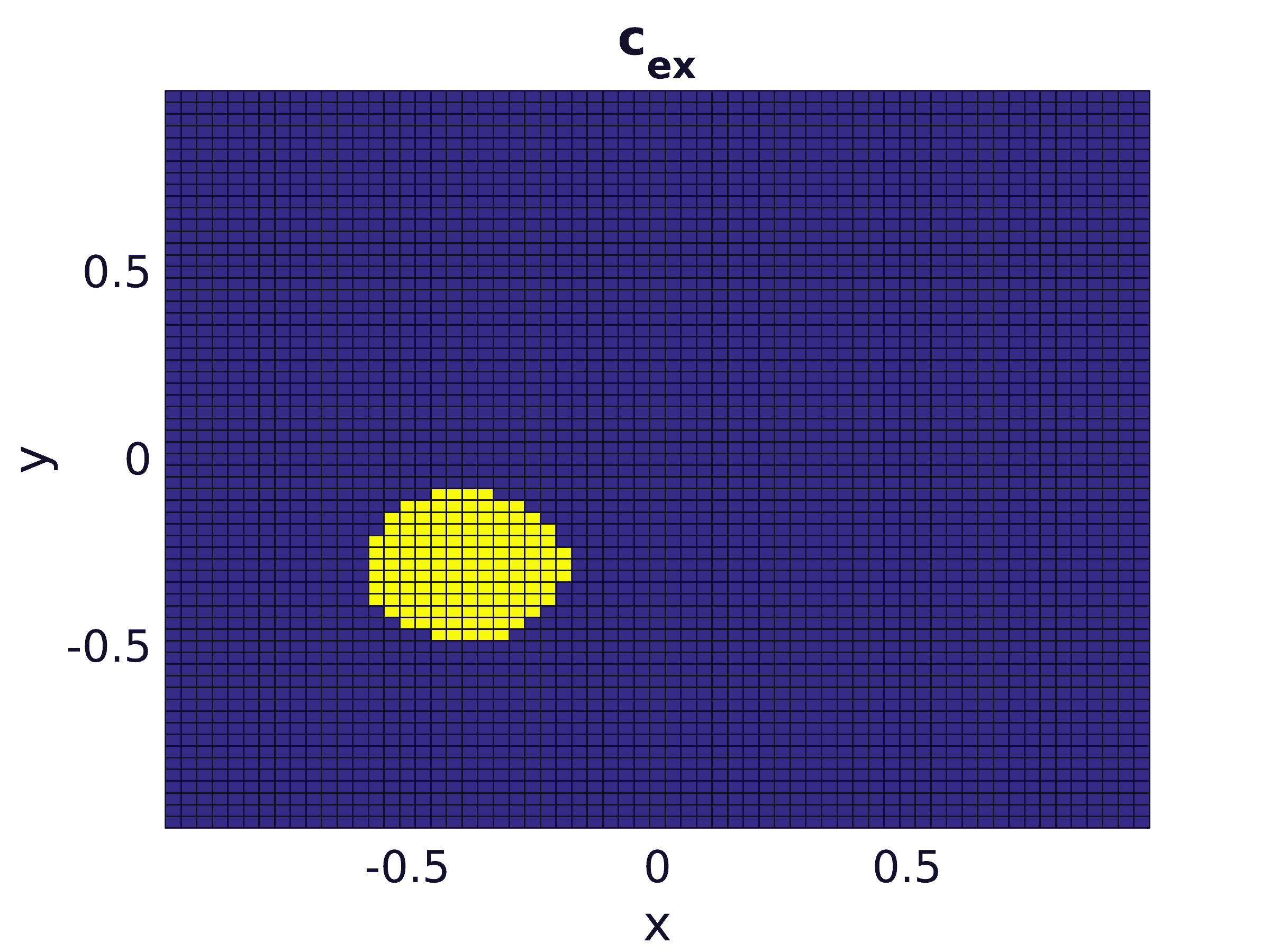
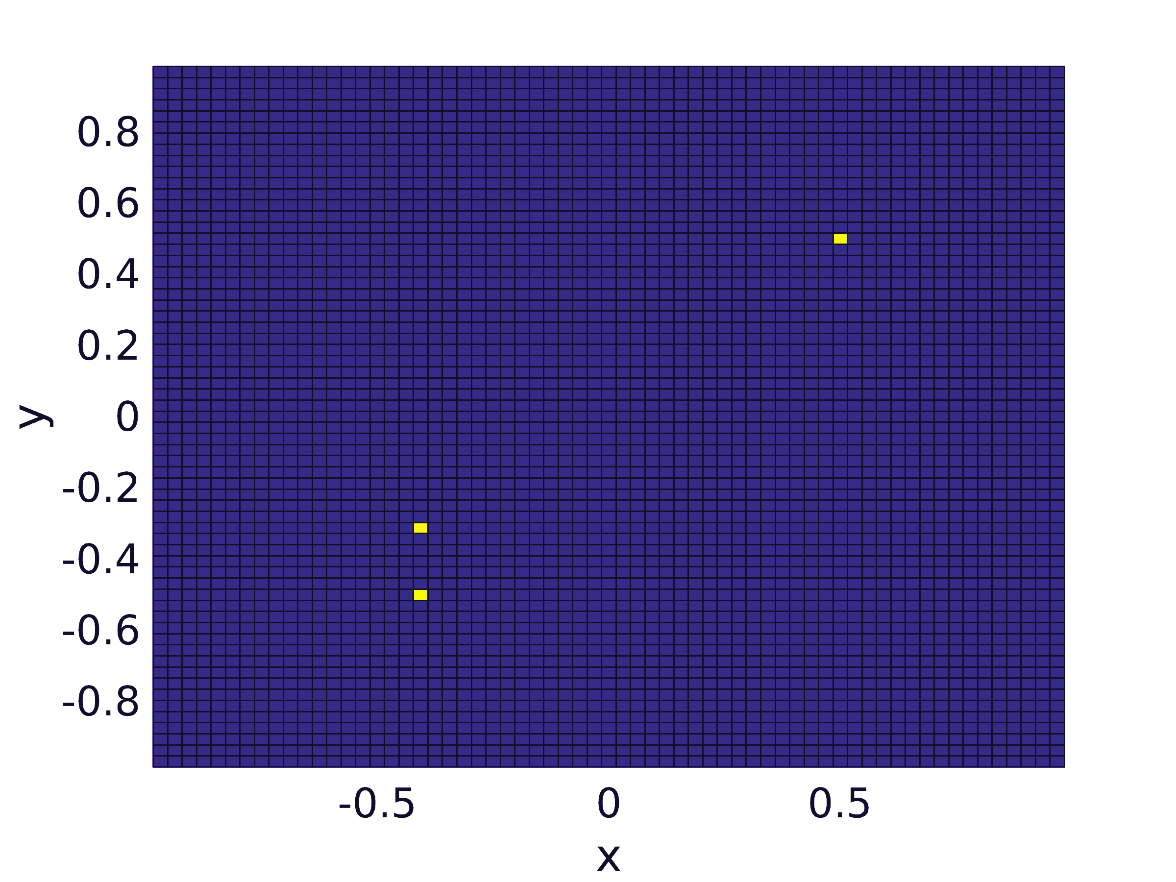
Figure 1: Left: exact coefficient ${b_{f}}_{ex}=c_{ex}=a_{ex}$. Right: locations of spots for testing weak * $L^{\infty}$ convergence.

The finite element grid used in computations was determined by subdividing the unit interval into $N=32$ subintervals in both directions, leading to $(N+1)^{2}=1089$ gridpoints for the piecewise linear nodal discretization of $u$ and $b_{f}$, as well as $2*N^{2}=2048$ triangles for the piecewise constant element discretization $c$ and $a$. Thus in the example from Section 3.1 we end up with $n=2178$, in the two other examples with $n=3137$ unknowns. Part of the experiments were also carried out on a finer grid with $N=64$ and correspondingly $n=8450$ or $n=12417$ unknowns. In order to avoid an inverse crime, we generated the synthetic data on a finer grid for the example from Section 3.1, while in the examples from Sections 3.2, 3.3, we additionally prescribed the exact state as $\phi_{ex}(x,y)=\cos(\frac{\pi}{2}x)\sin(\frac{\pi}{2}y)$, and computed the corresponding right hand side $f$ on the finer grid. After projection of $\phi_{ex}$ onto the computational grid, we added uniformly distributed random noise of levels $\delta\in\{0.001,0.01,0.1\}$ corresponding to $0.1$, $1$ and $10$ per cent noise, to obtain synthetic data $y^{\delta}$. In all tests we started with the constant function with value $5.5$ for ${b_{f}}_{0},c_{0},a_{0}$ (i.e., the mean value between upper and lower bound) and $\phi_{0}\equiv y^{\delta}$. Moreover, we always set $\tau=1.1$.

First of all, we provide a comparison of the methods described in Section 5, in their Matlab implementations Feas_AS [7] and Infeas_AS [8] with quadprog which is the standard Matlab function for solving (31). The trust-region-reflective algorithm quadprog is a subspace trust-region method based on the interior-reflective Newton method from [5]. To facilitate transparency of our numerical tests we provide the Matlab code for generating and solving all instances with the various methods discussed in this paper under http://philipphungerlaender.com/qp-code/.

Table 3 shows the CPU times measured with the Matlab function cputime, the $L^{1}$ errors as well as the errors in certain spots within the two homogeneous regions and on their interface,

$$\mbox{spot}_{1}=(0.5,0.5)\,,\quad\mbox{spot}_{2}=(-0.4,-0.3)\,,\quad\mbox{spot}_{3}=(-0.4,-0.5)\,,$$

cf. Figure 1, more precisely, on $\frac{1}{N}\times\frac{1}{N}$ squares located at these spots, corresponding to the piecewise constant $L^{1}$ functions with these supports in order to exemplarily test weak * convergence. Moreover, we provide the number $k$ of Gauss Newton SQP iterations (which is always one in the linear inverse source problem, of course) and the relative residual, i.e., the cost function ratio at the final iterate $\frac{J(x_{k}^{\delta},u_{k}^{\delta})}{J(x_{0},u_{0})}$. We do so for the three examples from Sections 3.1, 3.2, and 3.3, shortly referred to as “source”, “potential”, and “diffusion”, respectively, using the lowest noise level $\delta=0.001$ and, besides the discretization with $N=32$, also one with $N=64$ subintervals in both directions.

	source
	N=32 (n=2178)			N=64 (n=8450)
	quadprog	Infeas_AS	Feas_AS	quadprog	Infeas_AS	Feas_AS
$k$	1	1	1	1	1	1
$\frac{J(x_{k}^{\delta},u_{k}^{\delta})}{J(x_{0},u_{0})}$	6.6901e-06	6.6154e-06	6.6154e-06	3.2887e-05	3.2532e-05	3.2744e-05
$\mbox{err}_{spot_{1}}$	2.4023e-06	0	0	6.7780e-07	0	0
$\mbox{err}_{spot_{2}}$	7.3665e-06	0	0	0.0462	0	0
$\mbox{err}_{spot_{3}}$	1.0890e-05	0	0	1.3992	1.3917	1.3917
$\mbox{err}_{L^{1}(\Omega)}$	0.0462	0.0465	0.0465	0.0832	0.0834	0.0834
CPU	1.68	1.16	1.09	29.62	112.97	22.85
	potential
	N=32 (n=3137)			N=64 (n=12417)
	quadprog	Infeas_AS	Feas_AS	quadprog	Infeas_AS	Feas_AS
$k$	4	4	6	3	3	3
$\frac{J(x_{k}^{\delta},u_{k}^{\delta})}{J(x_{0},u_{0})}$	6.2155e-06	6.0569e-06	8.0316e-07	1.6318e-04	1.6286e-04	1.6286e-04
$\mbox{err}_{spot_{1}}$	6.9611e-10	0	0	1.2184e-10	0	0
$\mbox{err}_{spot_{2}}$	1.7502e-06	0	0	0.7183	0.7145	0.7145
$\mbox{err}_{spot_{3}}$	1.5392	1.6093	1.4363	3.2625	3.2629	3.2629
$\mbox{err}_{L^{1}(\Omega)}$	0.1051	0.1044	0.0938	0.1460	0.1444	0.1444
CPU	21.88	24.44	18.34	432.06	368.67	276.17
	diffusion
	N=32 (n=3137)			N=64 (n=12417)
	quadprog	Infeas_AS	Feas_AS	quadprog	Infeas_AS	Feas_AS
$k$	4	4	4	8	8	8
$\frac{J(x_{k}^{\delta},u_{k}^{\delta})}{J(x_{0},u_{0})}$	0.0931	0.0931	0.0931	0.0543	0.0543	0.0543
$\mbox{err}_{spot_{1}}$	3.7303e-14	0	0	3.6415e-14	0	0
$\mbox{err}_{spot_{2}}$	4.4418	4.4418	4.4418	7.8278e-05	0	0
$\mbox{err}_{spot_{3}}$	0.3200	0.3199	0.3199	4.3077e-13	0	0
$\mbox{err}_{L^{1}(\Omega)}$	0.3259	0.3259	0.3259	0.3799	0.3799	0.3799
CPU	32.01	6.30	5.25	1193.00	532.57	463.89

Table 3: Comparison of different solvers for QPs with box constraints.

We observe that Infeas_AS and Feas_AS obviously reach the same solution, which is almost bang-bang, as the vanishing errors in almost all spots show, whereas quadprog, being an interior point method, exhibits small deviations from the bounds. In all cases Feas_AS outperforms the other two methods as far as CPU times are concerned. Therefore the following computations were done using Feas_AS.

To provide an illustration of convergence as the noise level tends to zero, we performed five runs on each noise level for each example and list the average errors in Table 4. In the diffusion example, where we need to regularize, we set $\alpha=1.e-4\cdot\delta$. Correspondingly we provide an illustration of the convergence history for the inverse potential problem from Section 3.2 for two different noise levels $\delta=0.1$ and $\delta=0.01$ in Figures 2, 3.

	source			potential			diffusion
$\delta$	0.001	0.01	0.1	0.001	0.01	0.1	0.001	0.01	0.1
$\mbox{err}_{spot_{1}}$	0	0.2000	0.2000	0	0	0	0	0	0
$\mbox{err}_{spot_{2}}$	0	2.7488	4.0702	0	0.7960	4.8689	0	8.4141	9.8436
$\mbox{err}_{spot_{3}}$	0	0.5678	1.9445	1.0840	2.1512	2.5862	0.6572	0	0
$\mbox{err}_{L^{1}(\Omega)}$	0.0472	0.5288	0.5721	0.1472	0.2136	0.3671	0.7200	0.3783	0.3745

Table 4: Convergence as $\delta\to 0$: averaged errors of five test runs with uniform noise.

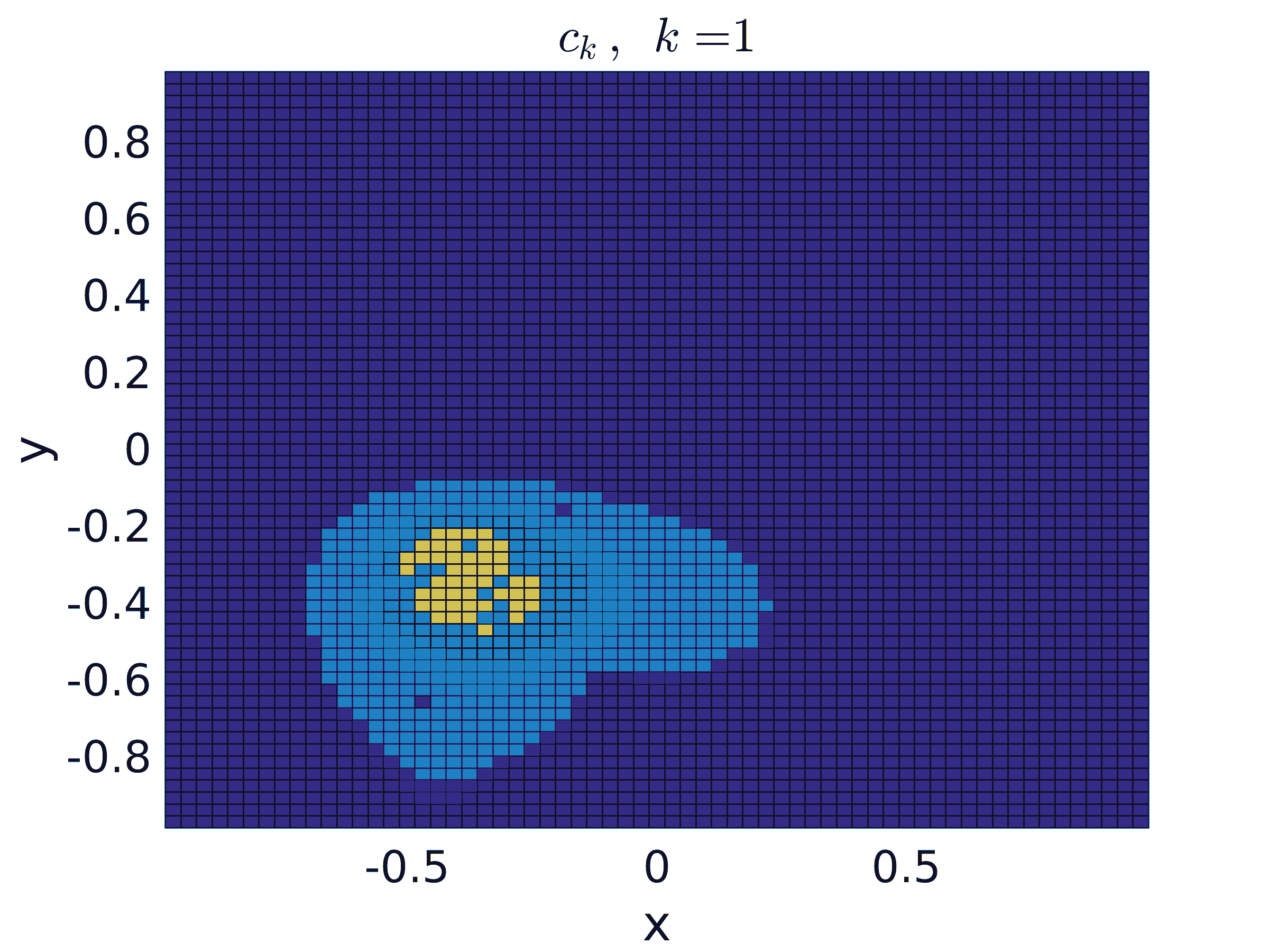
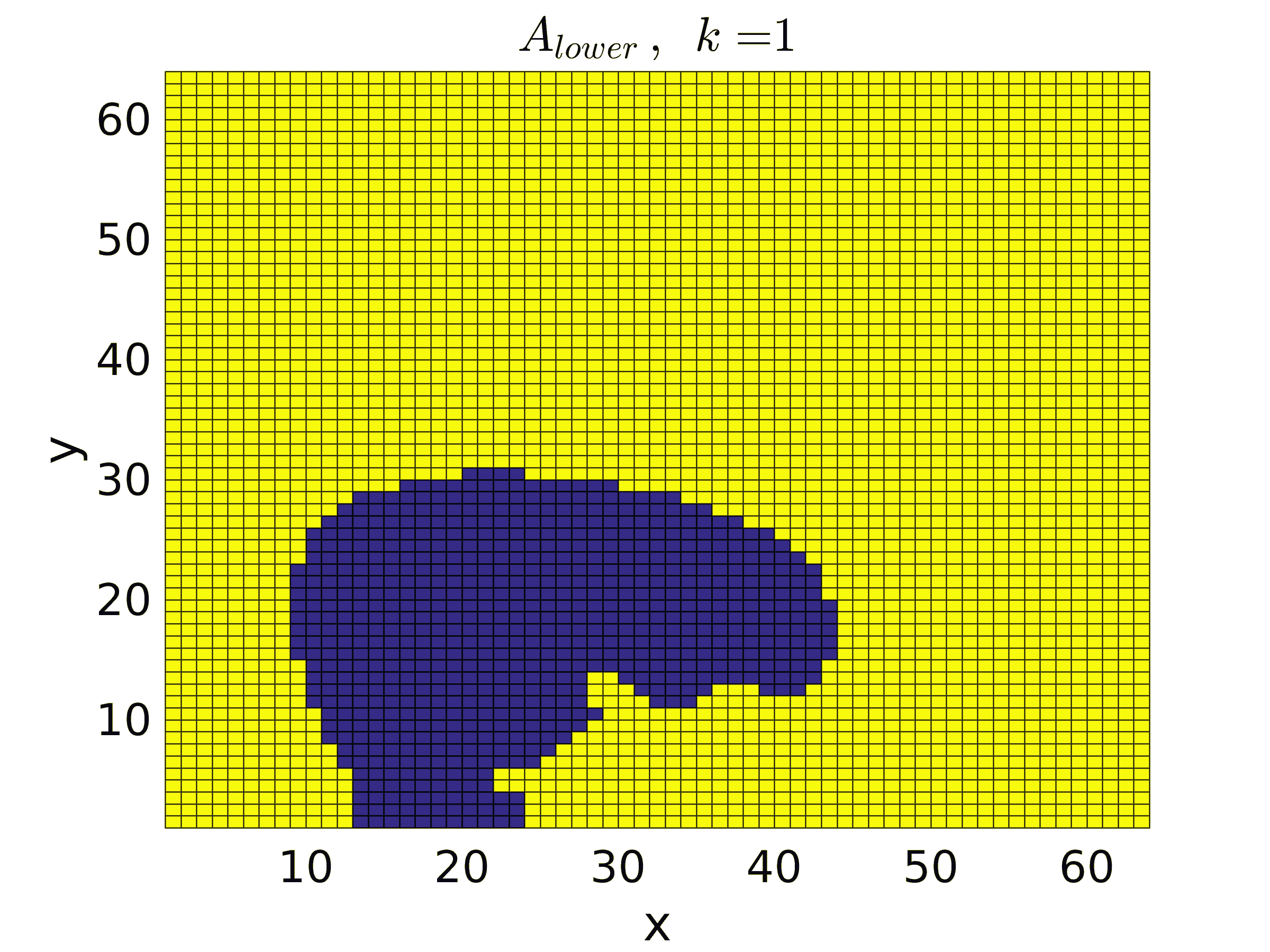
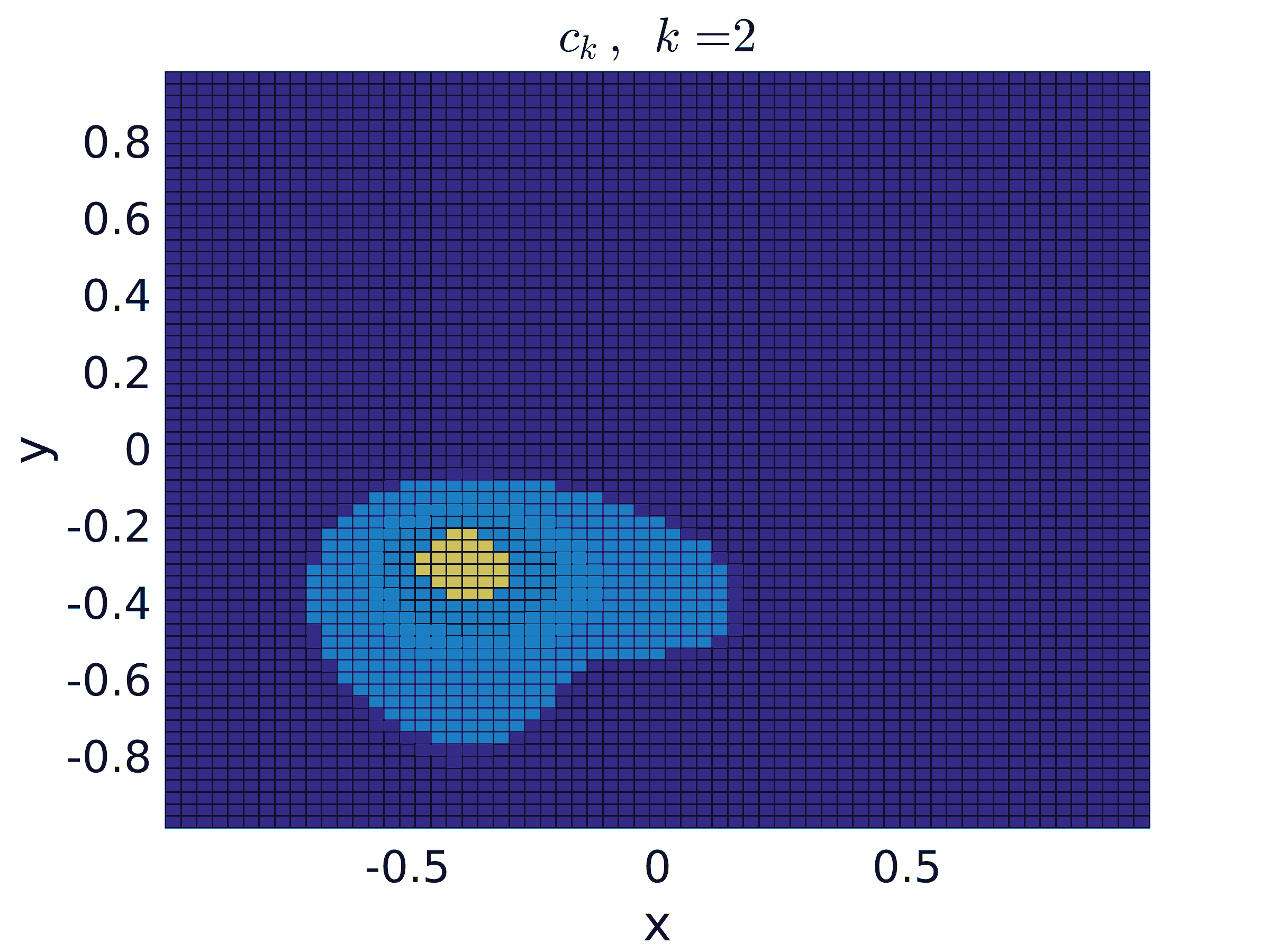
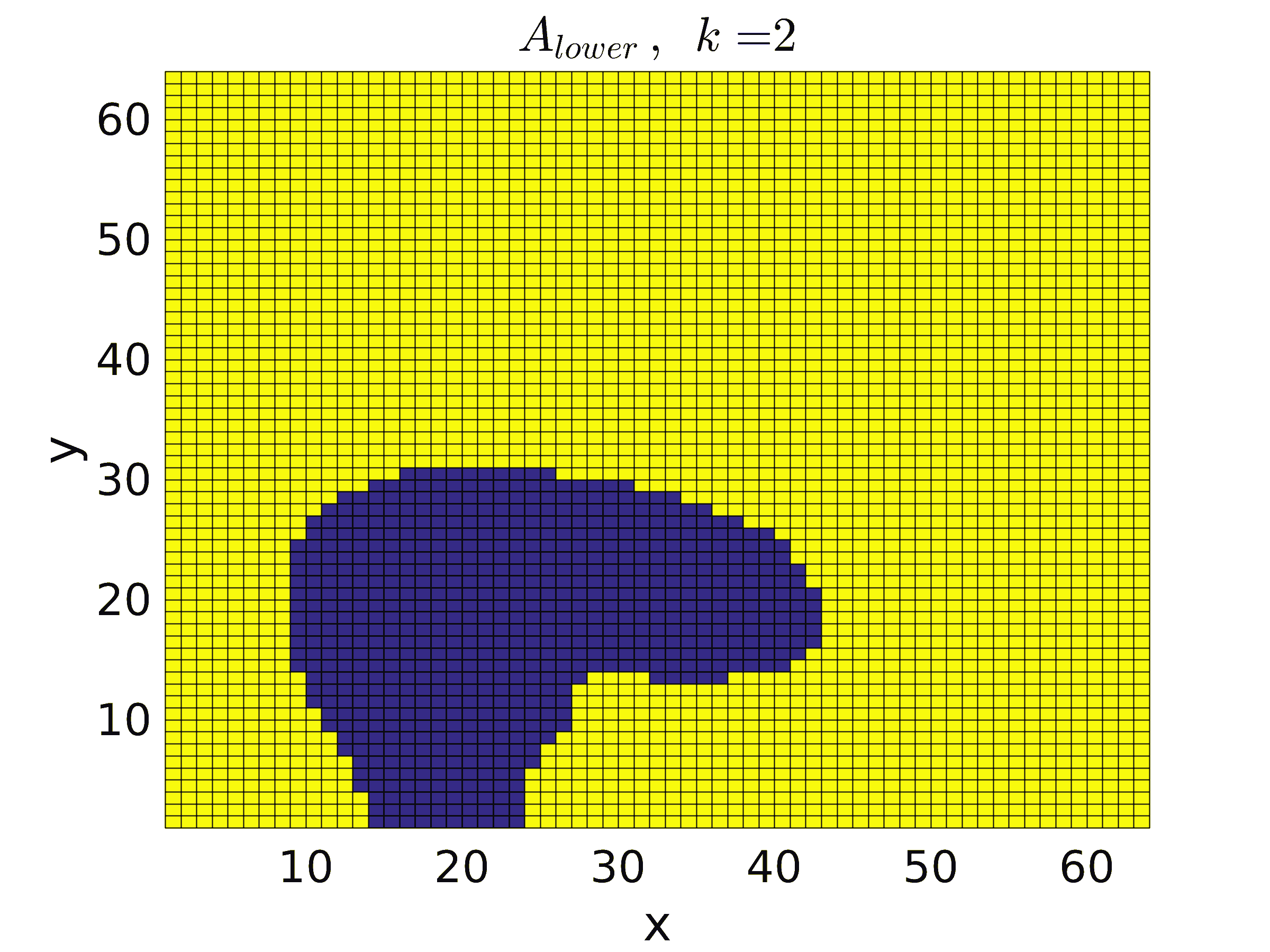
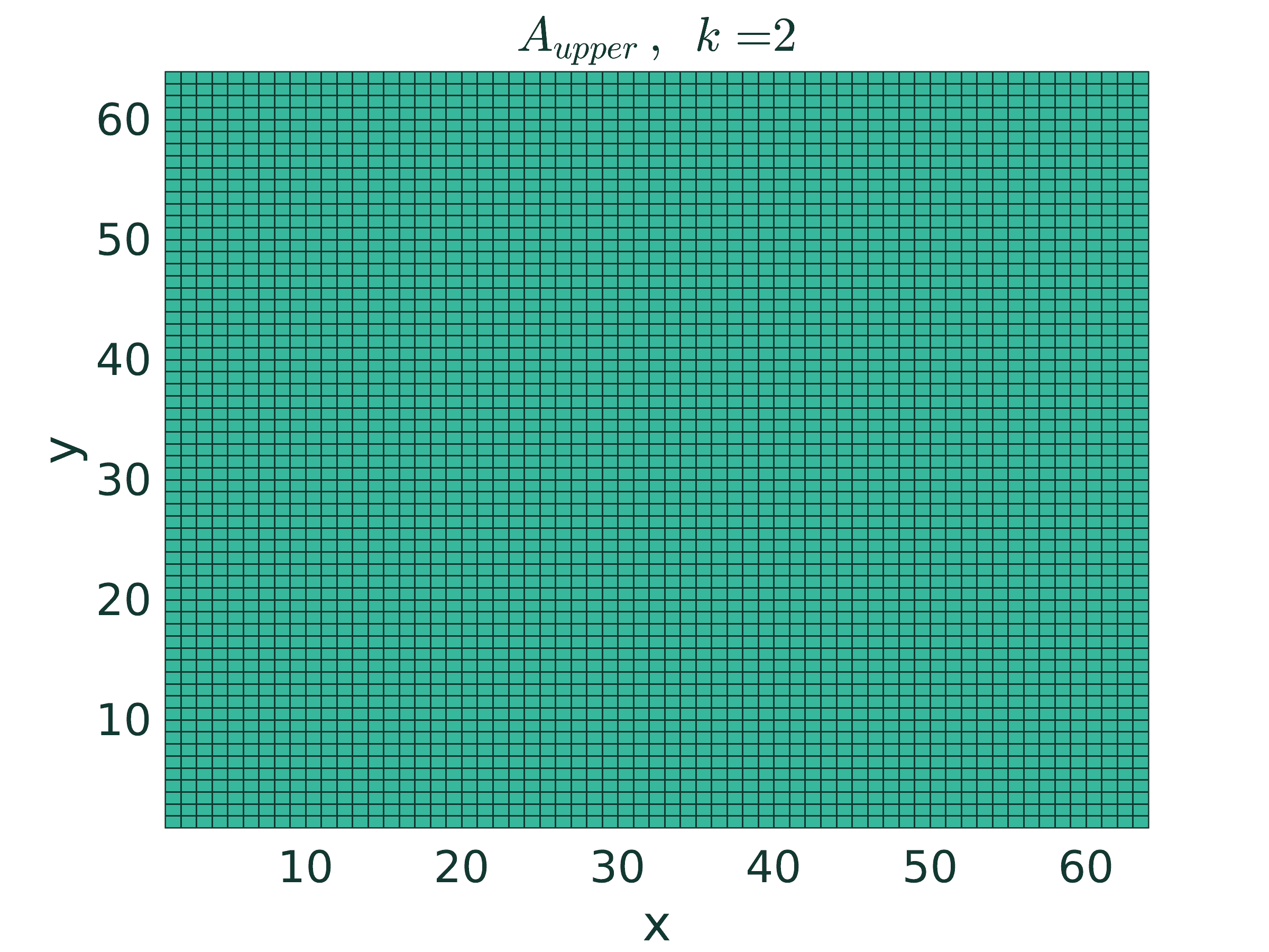
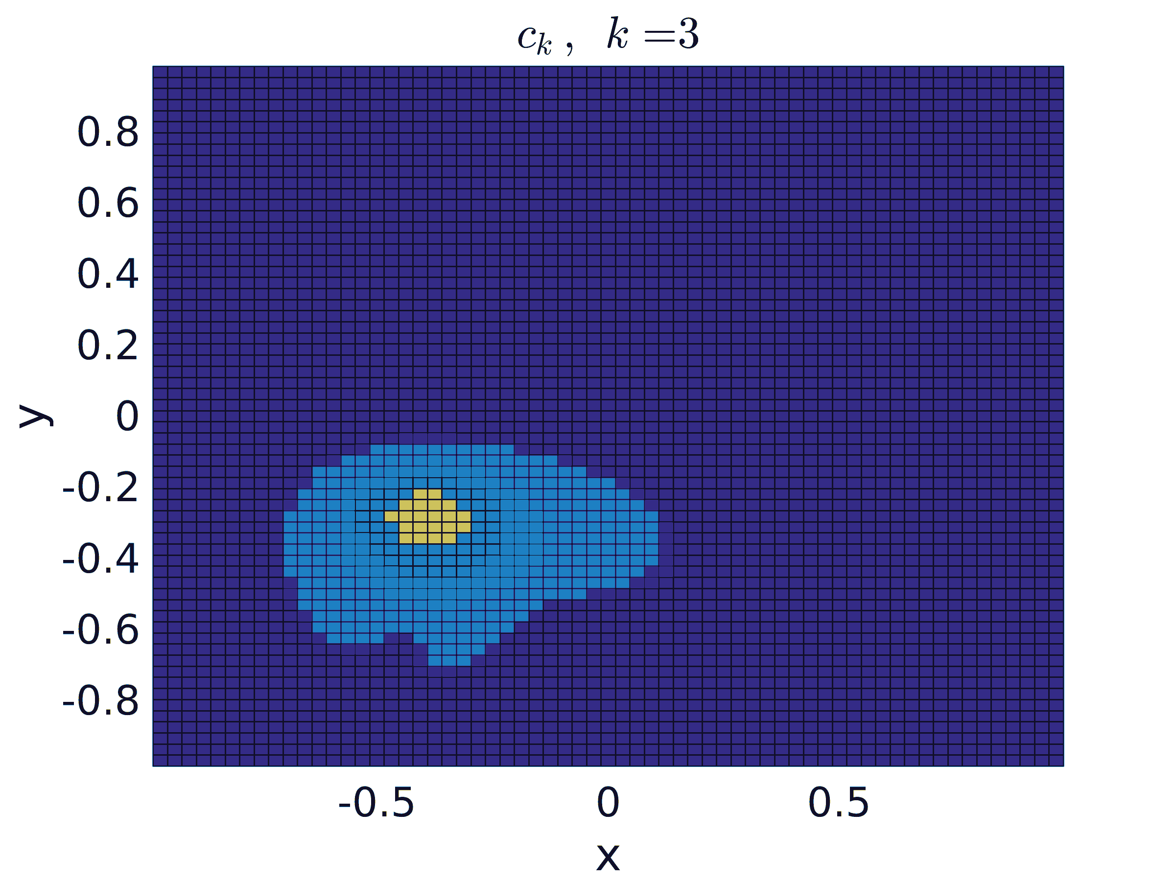
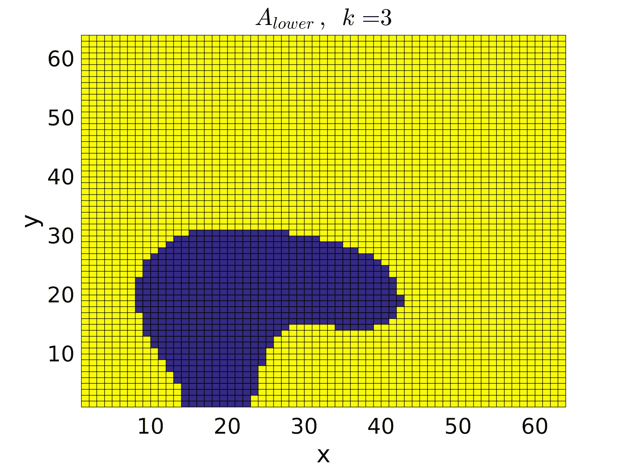
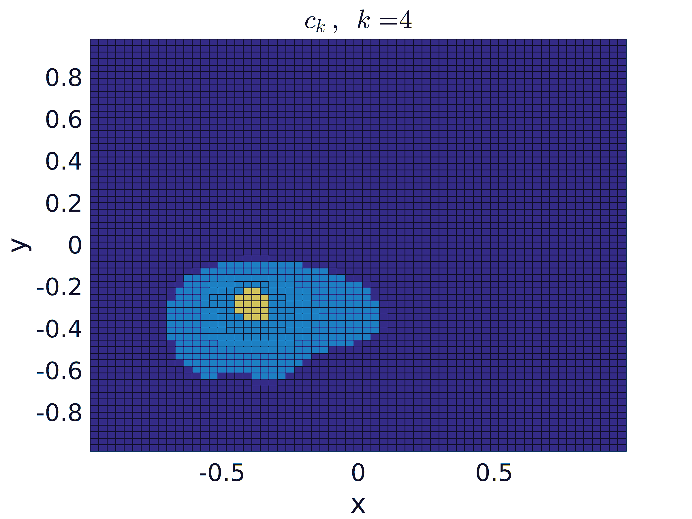
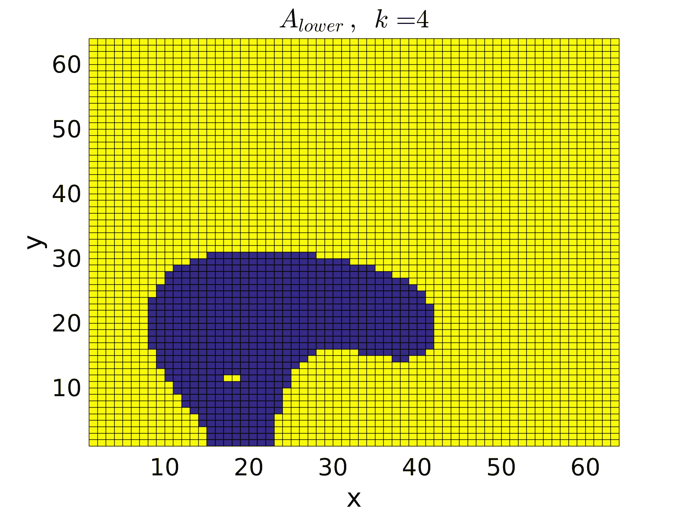
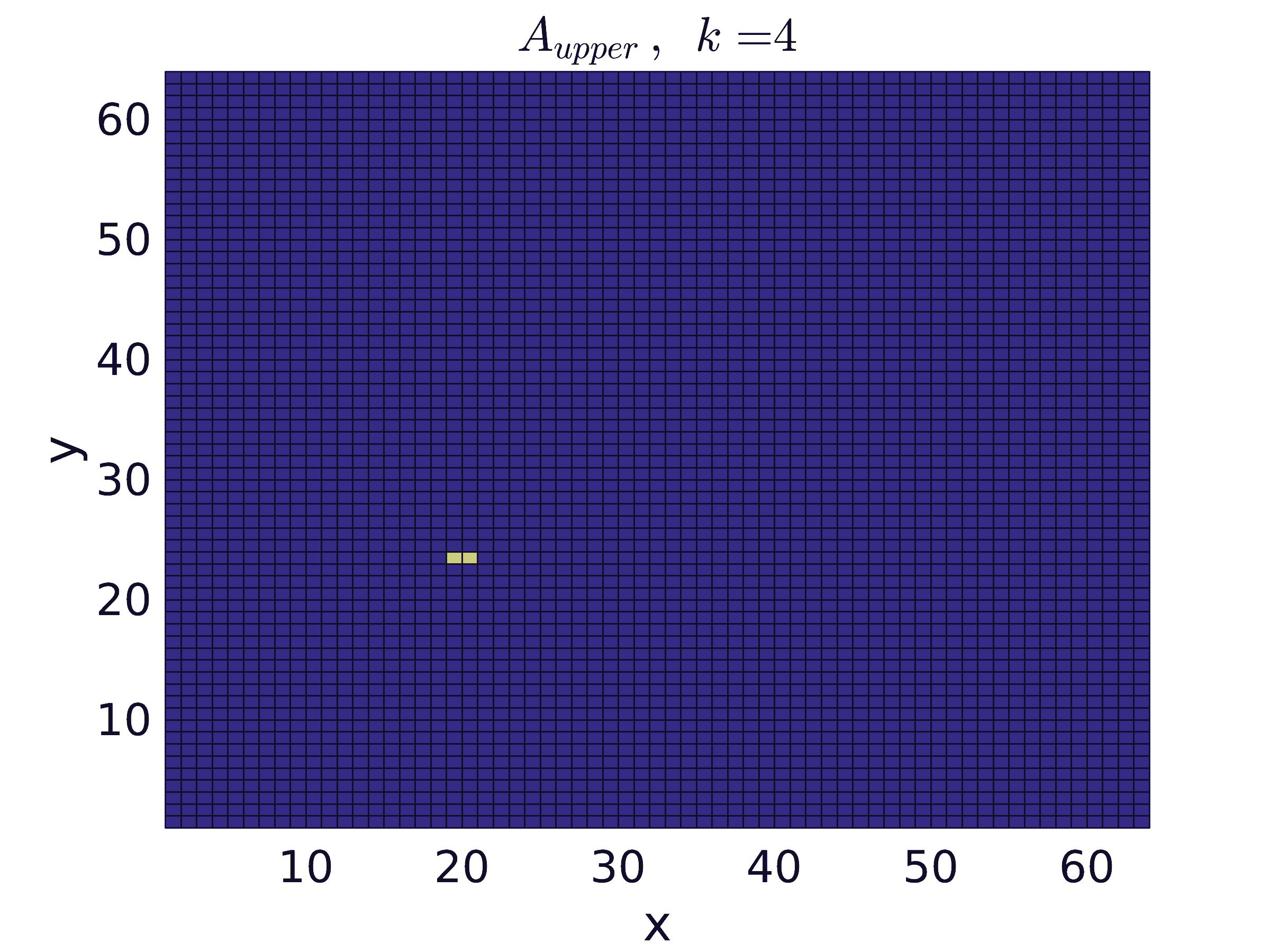
Figure 2: Left: reconstructed coefficient $c_{k}$; Middle: active set for lower bound; Right: active set for upper bound; For $k=1,2,3,4$ (top to bottom) and $\delta=0.1$.

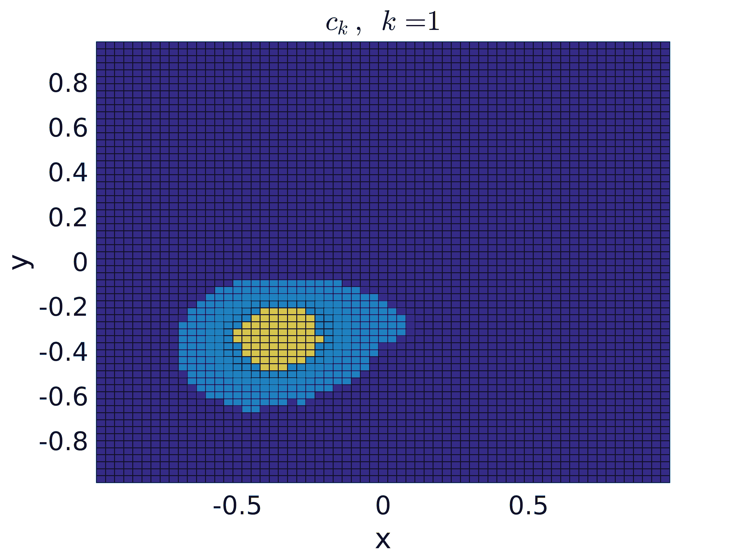
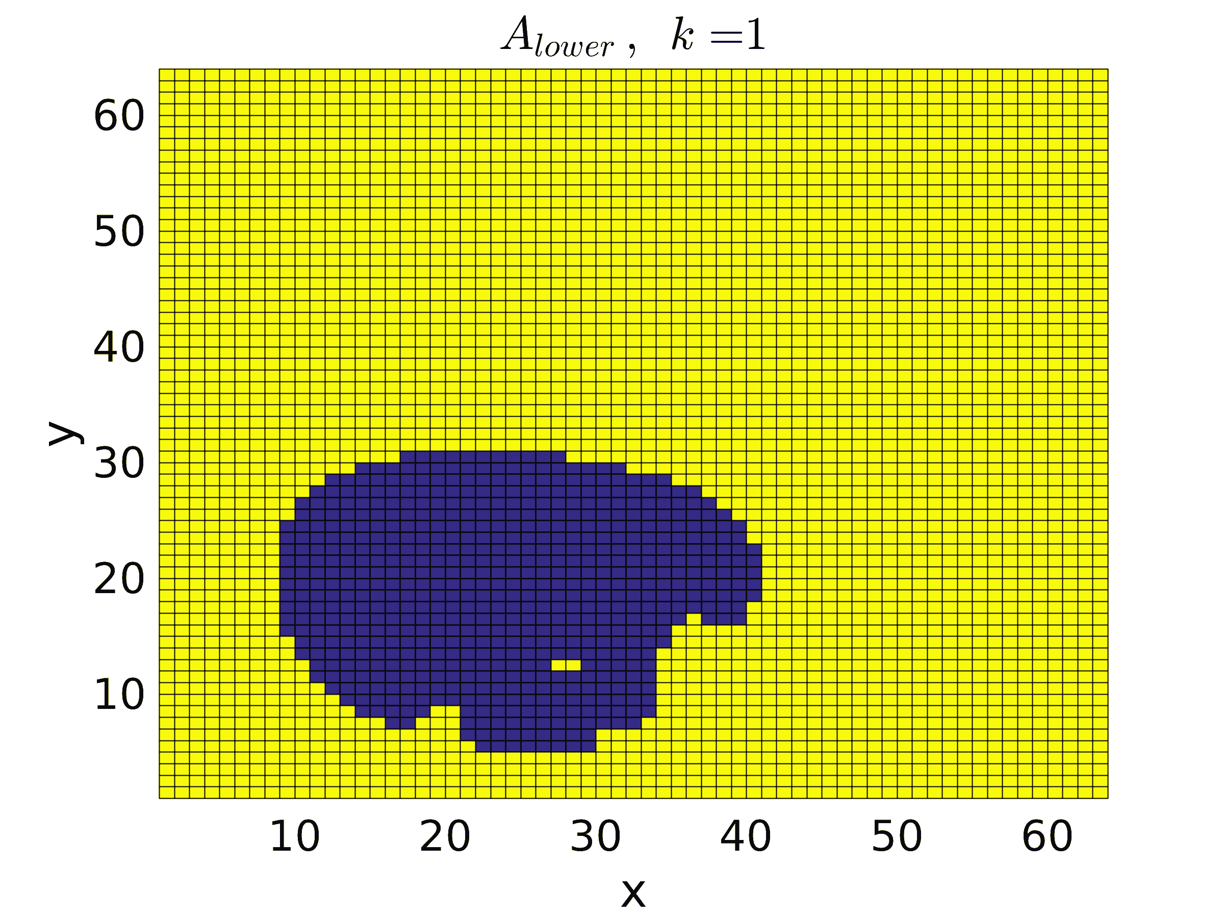
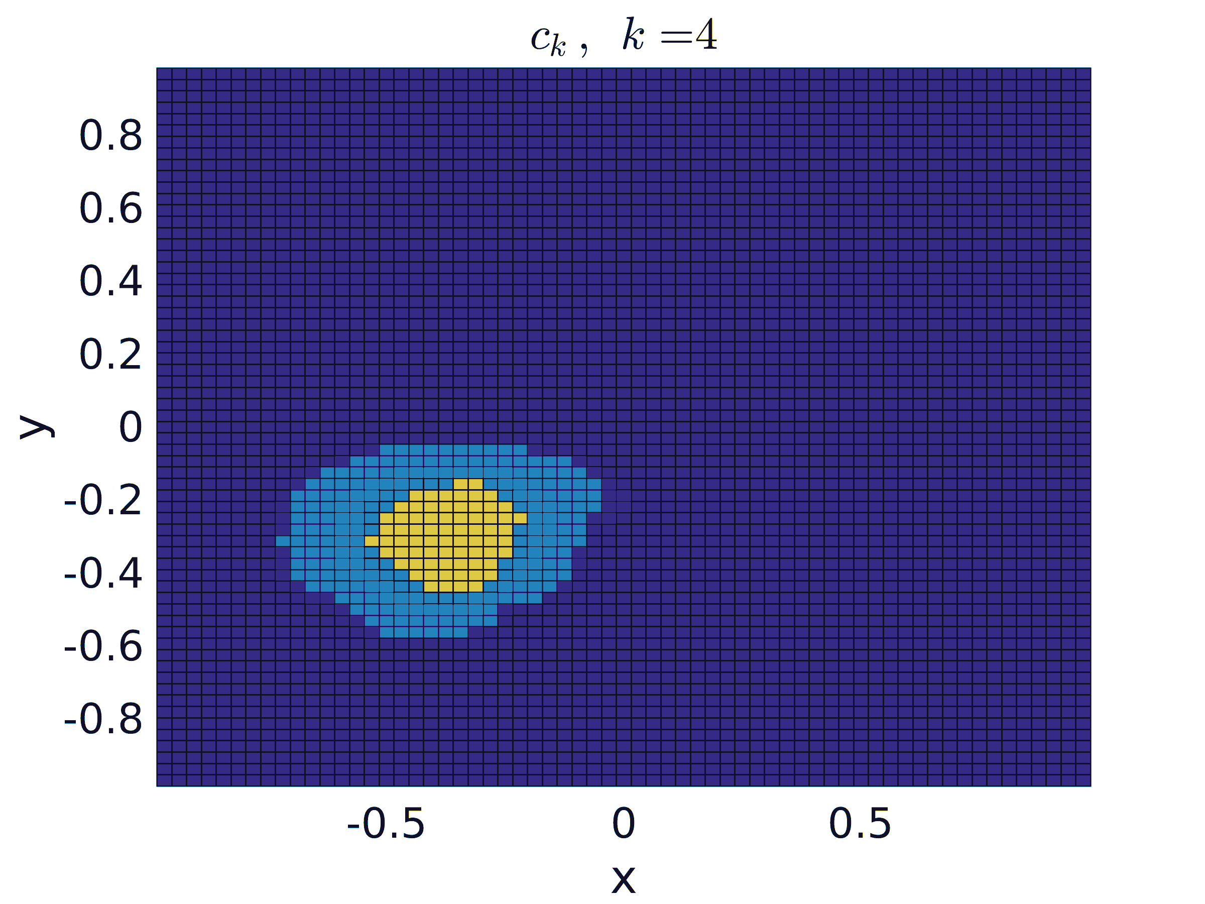
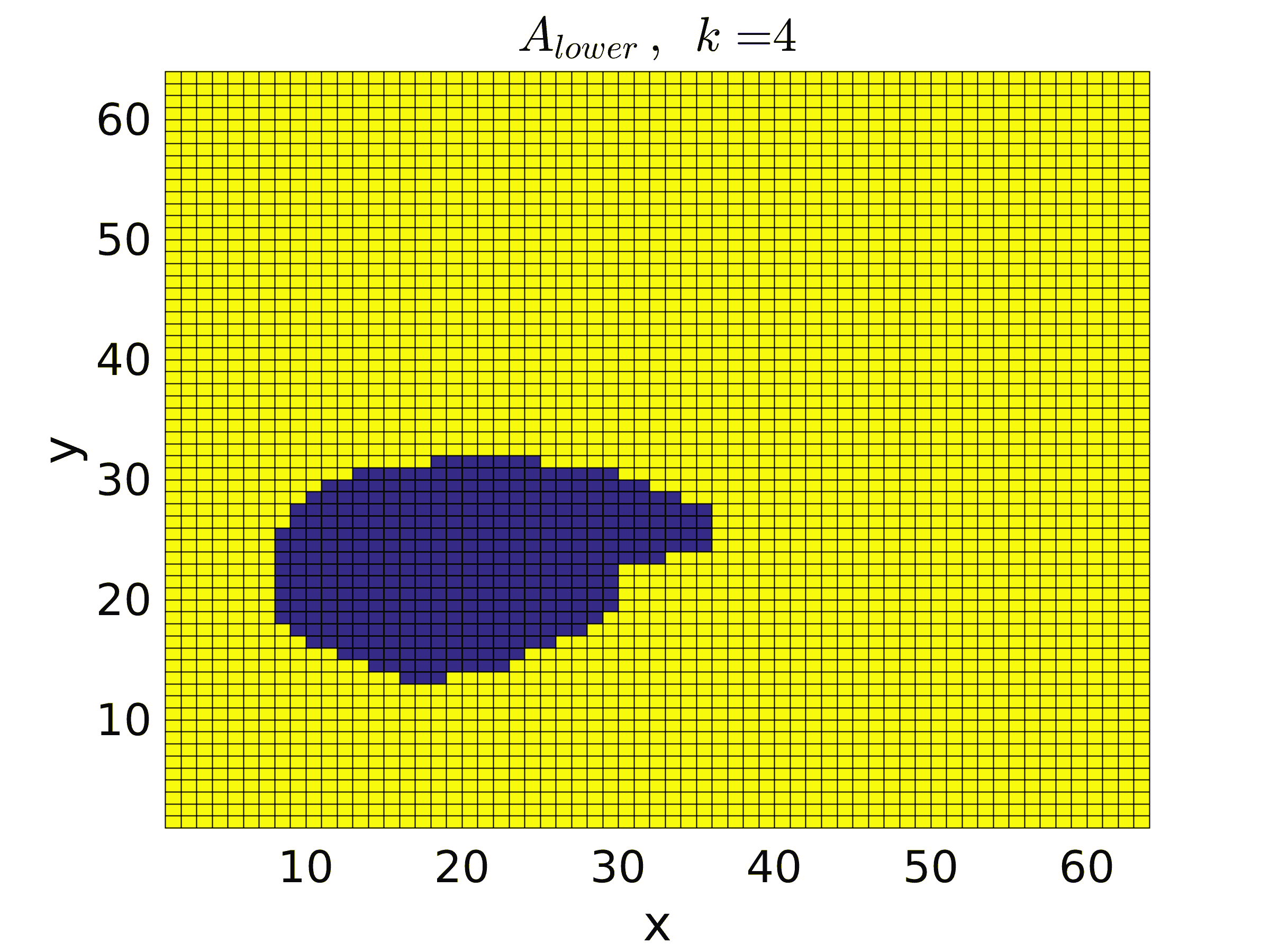
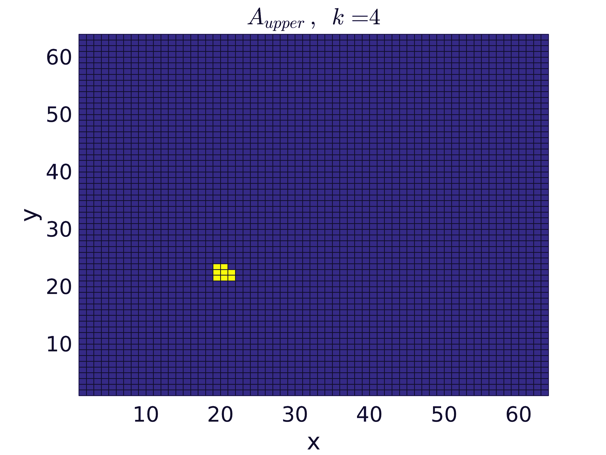
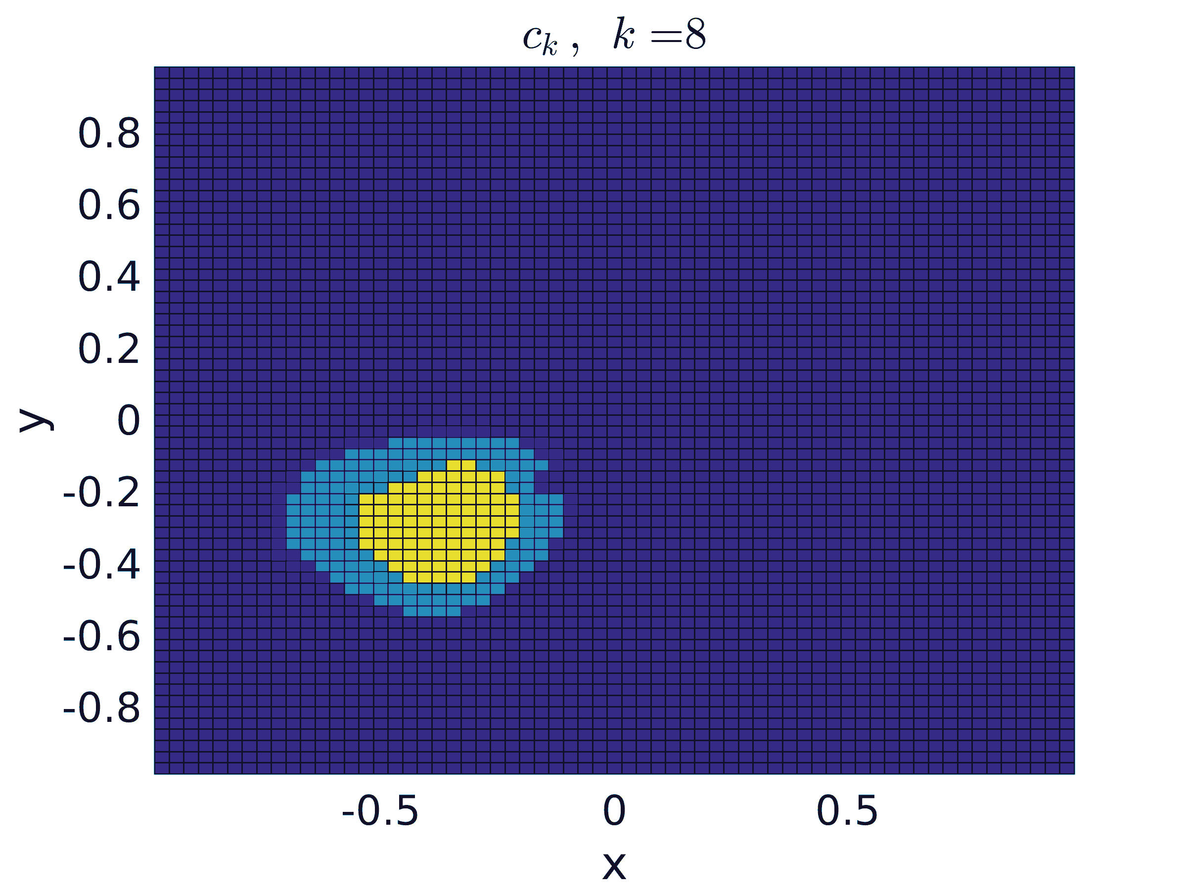
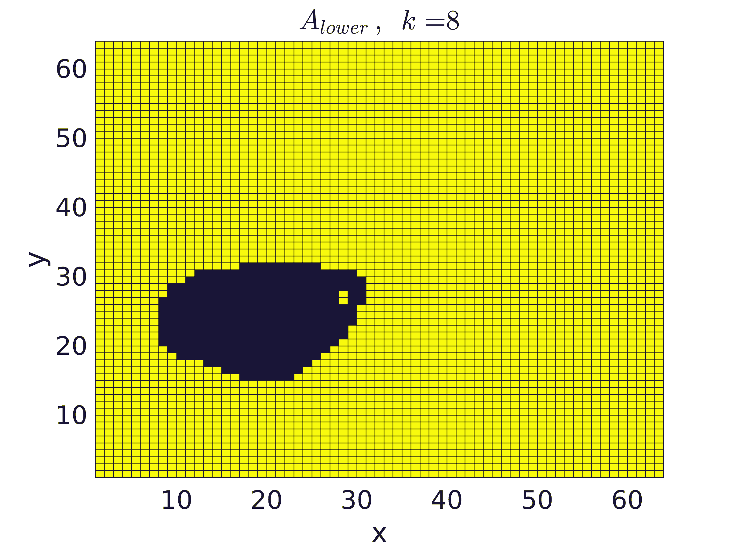
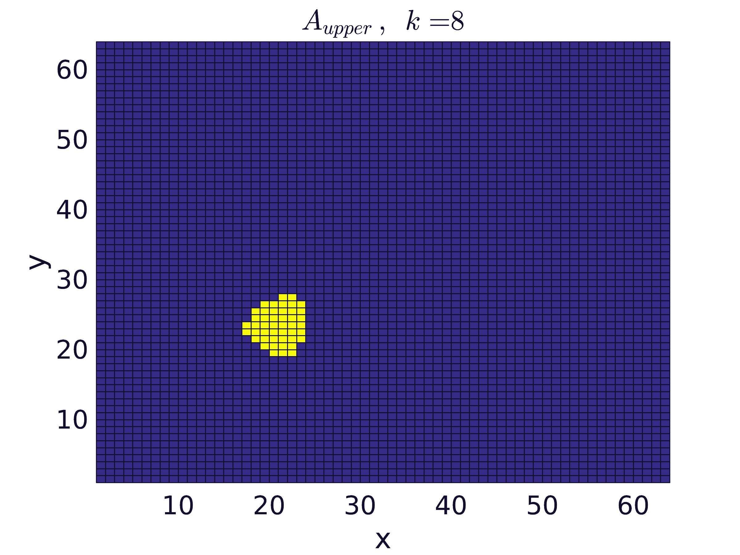
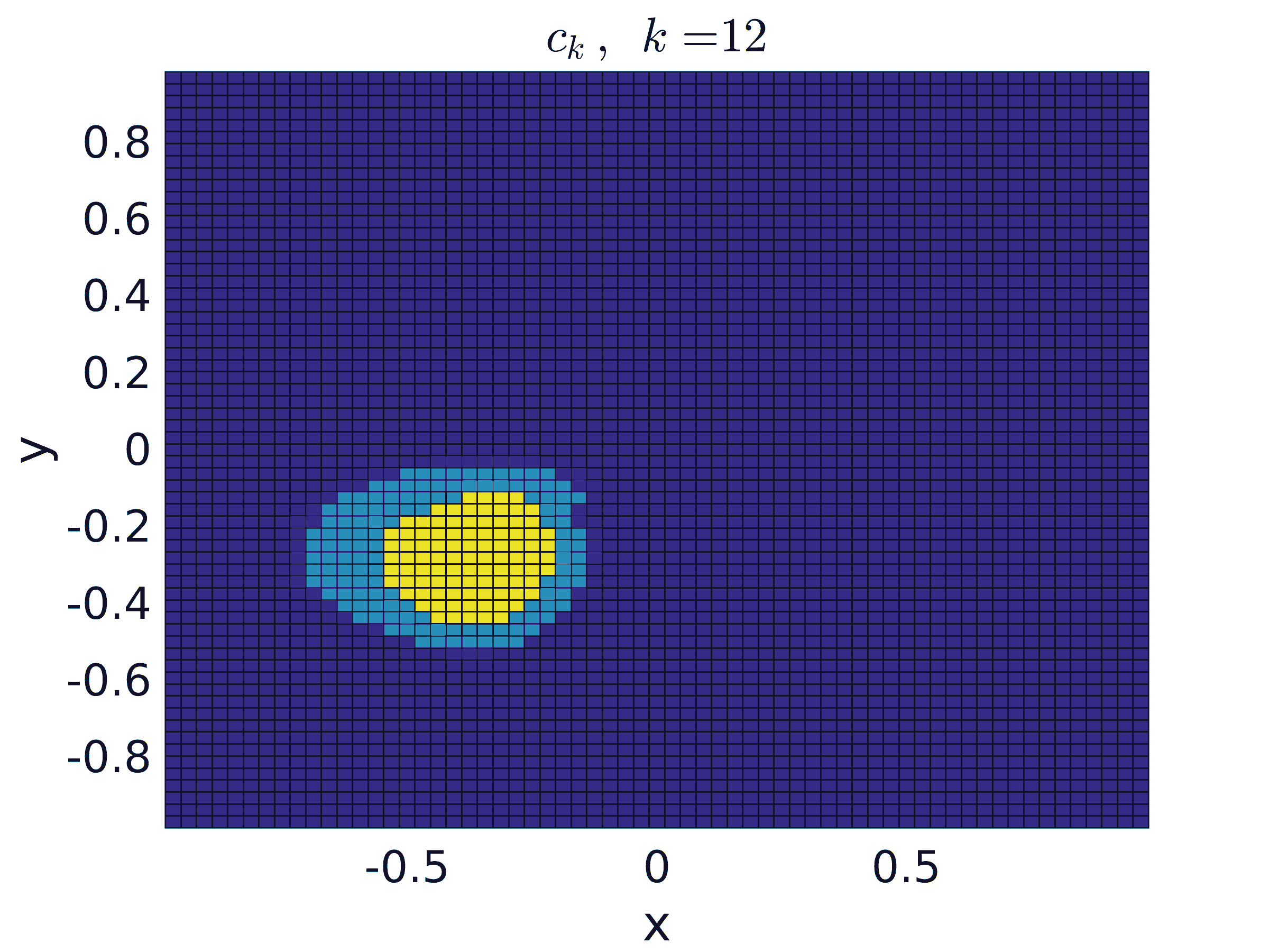
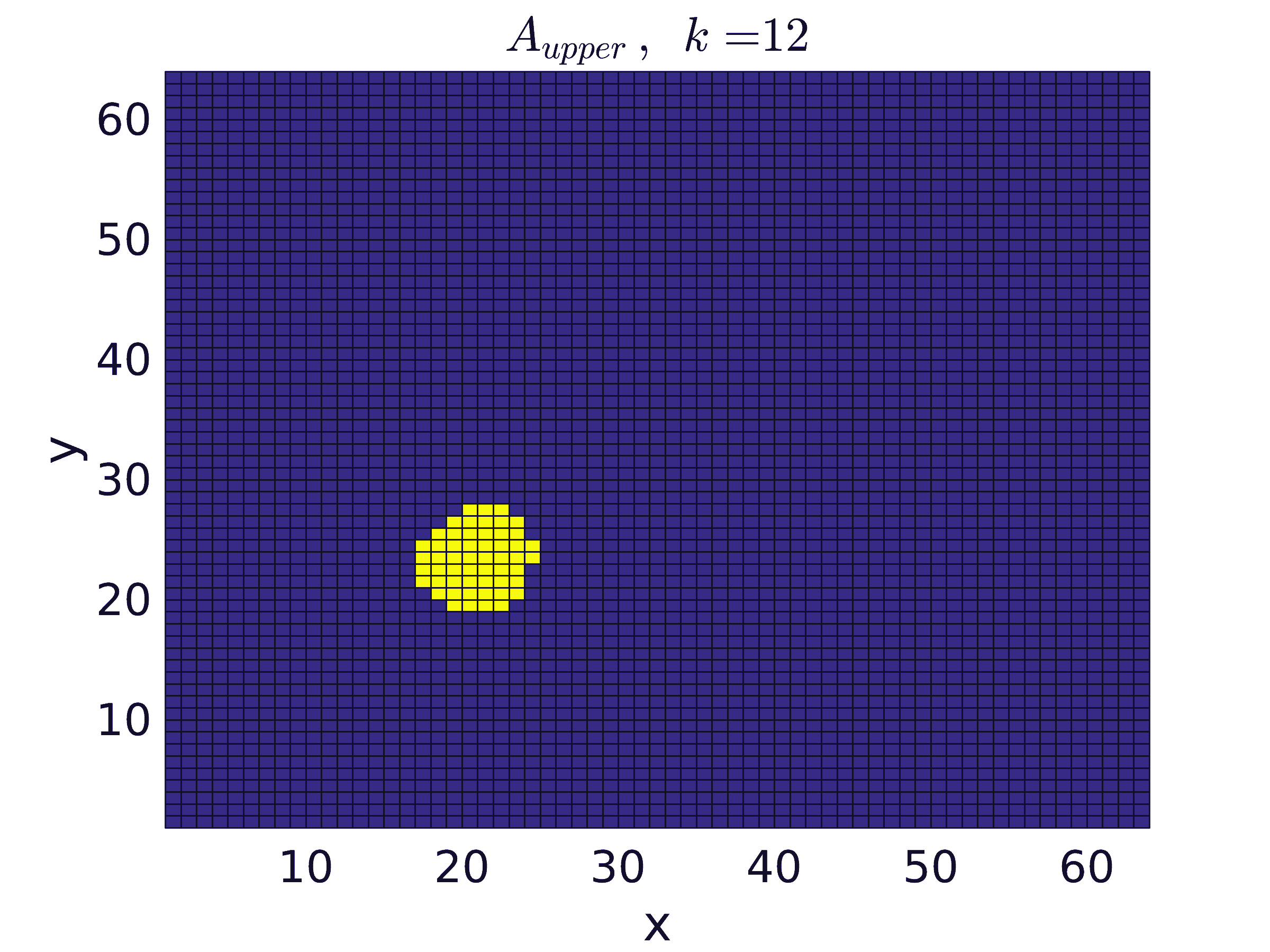
Figure 3: Left: reconstructed coefficient $c_{k}$; Middle: active set for lower bound; Right: active set for upper bound; For $k=1,4,8,12$ (top to bottom) and $\delta=0.01$.

Next, we consider a fixed noise level of $\delta=0.001$ and illustrate the gain in computational effort obtained by using the active set from the previous Newton step as an initial guess (warm start) as compared to starting each Newton step with an empty active set $\mathcal{A}=\emptyset$ for the upper bound and a full active set $\mathcal{C}=\mathcal{N}$ for the lower bound (cold start), see Figure 4. We do so for the inverse potential problem from Section 3.2. The CPU times were 8.60 (351.20) seconds with warm start and 9.15 (525.99) seconds with cold start to achieve an $L^{1}$ error of 0.0959 (0.0827) for N=32 (N=64).

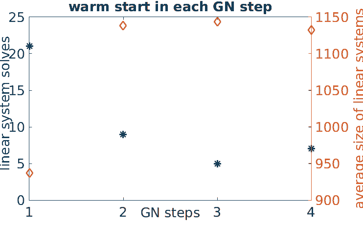
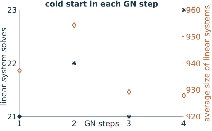
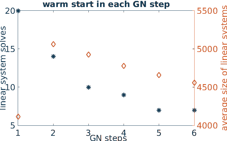
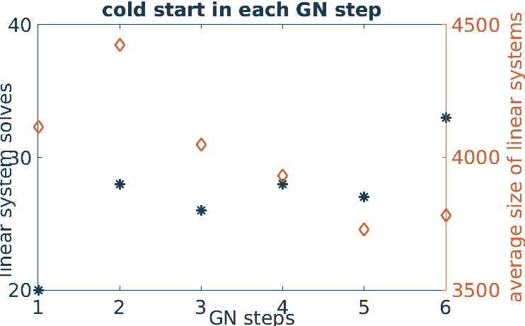
Figure 4: Linear system solves (stars) and average size of linear systems (diamonds); Left: warm start; Right: cold start; Top: N=32; Bottom: N=64.

Finally, in order to demonstrate the ability of the method to also deal with coefficients that would not allow for a well-defined parameter-to-state map, we consider the inverse potential problem from Section 3.2 with the test cases

$$\mbox{test 2: }c_{ex}(x,y)=1-10\cdot{1\!\!{\rm I}}_{B_{1}}+5\cdot{1\!\!{\rm I}}_{B_{2}} \underline{c}=-9, \overline{c}=6\,,$$

$$\mbox{test 3: }c_{ex}(x,y)=-10\cdot{1\!\!{\rm I}}_{B_{1}}-5\cdot{1\!\!{\rm I}}_{B_{2}} \underline{c}=-10, \overline{c}=0\,,$$

where $B_{1}=B_{0.2}(-0.4,-0.3)$, $B_{2}=B_{0.1}(0.5,0.5)$, see Figures 5, 6, 7, 8.

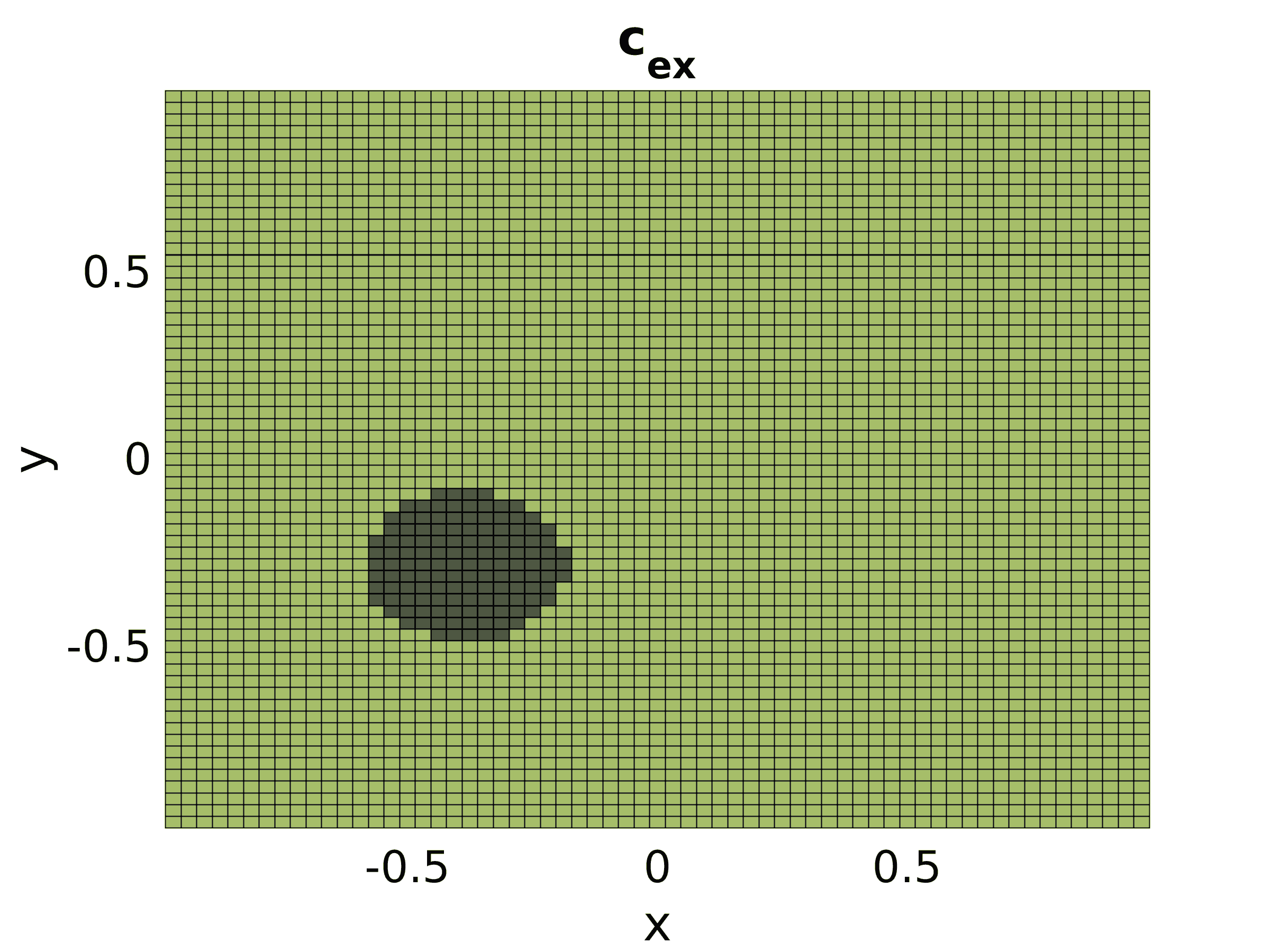
Figure 5: Test 2: left: exact coefficient $c_{ex}$; $\underline{c}=-9$, $\overline{c}=6$; right: locations of spots for testing weak * $L^{\infty}$ convergence

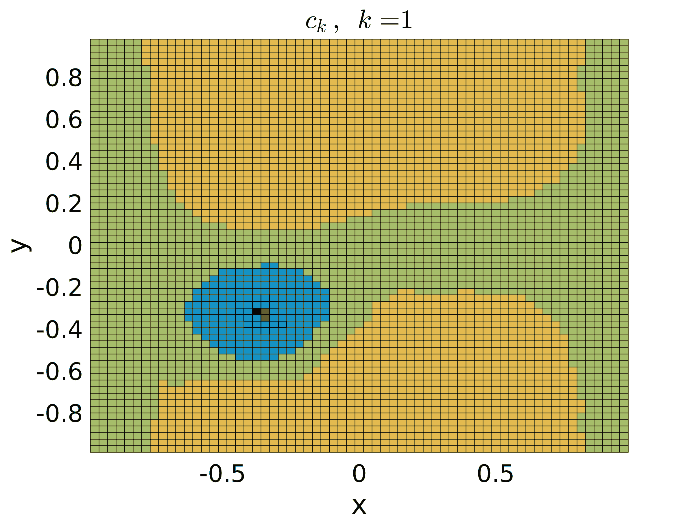
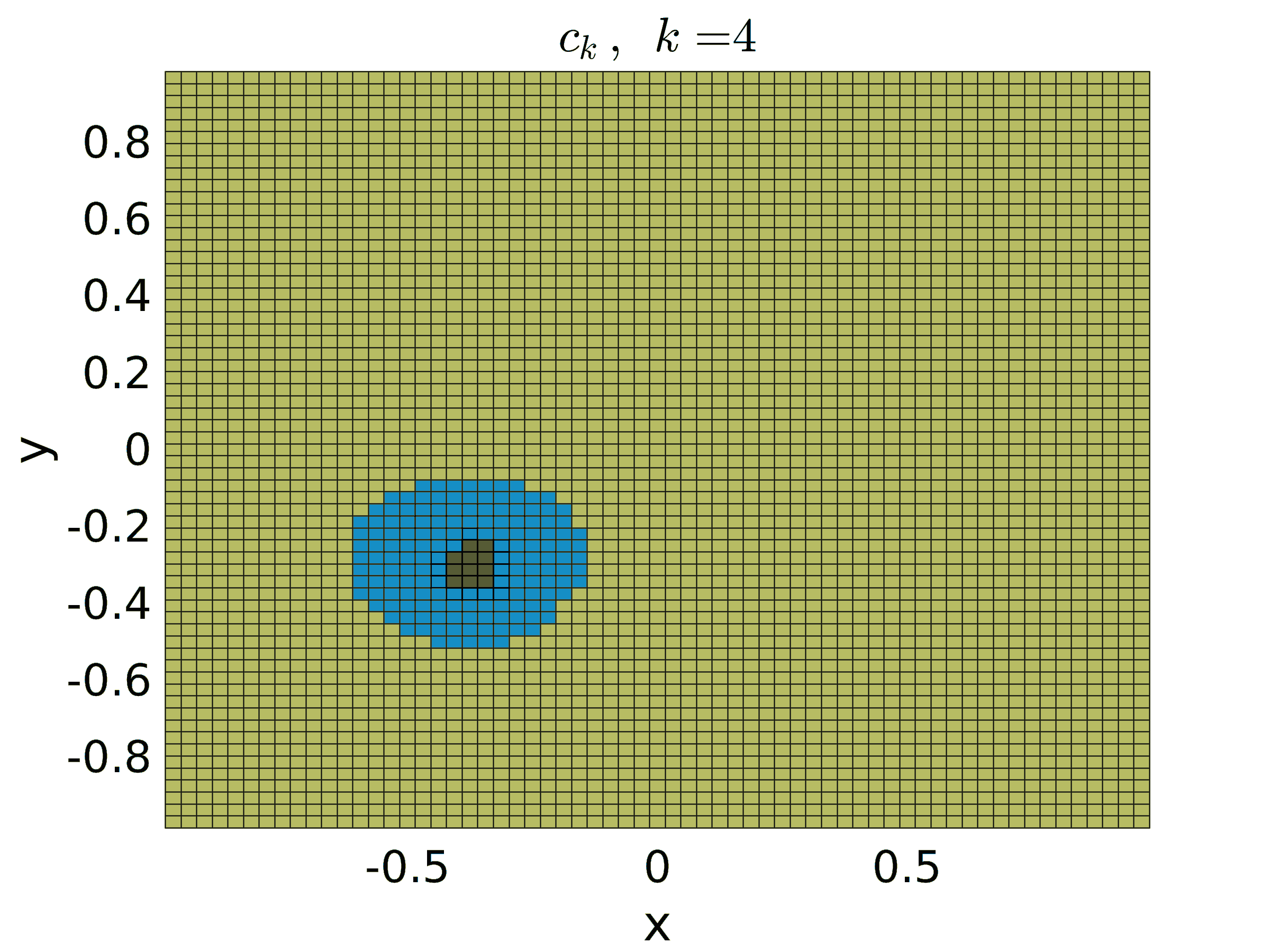
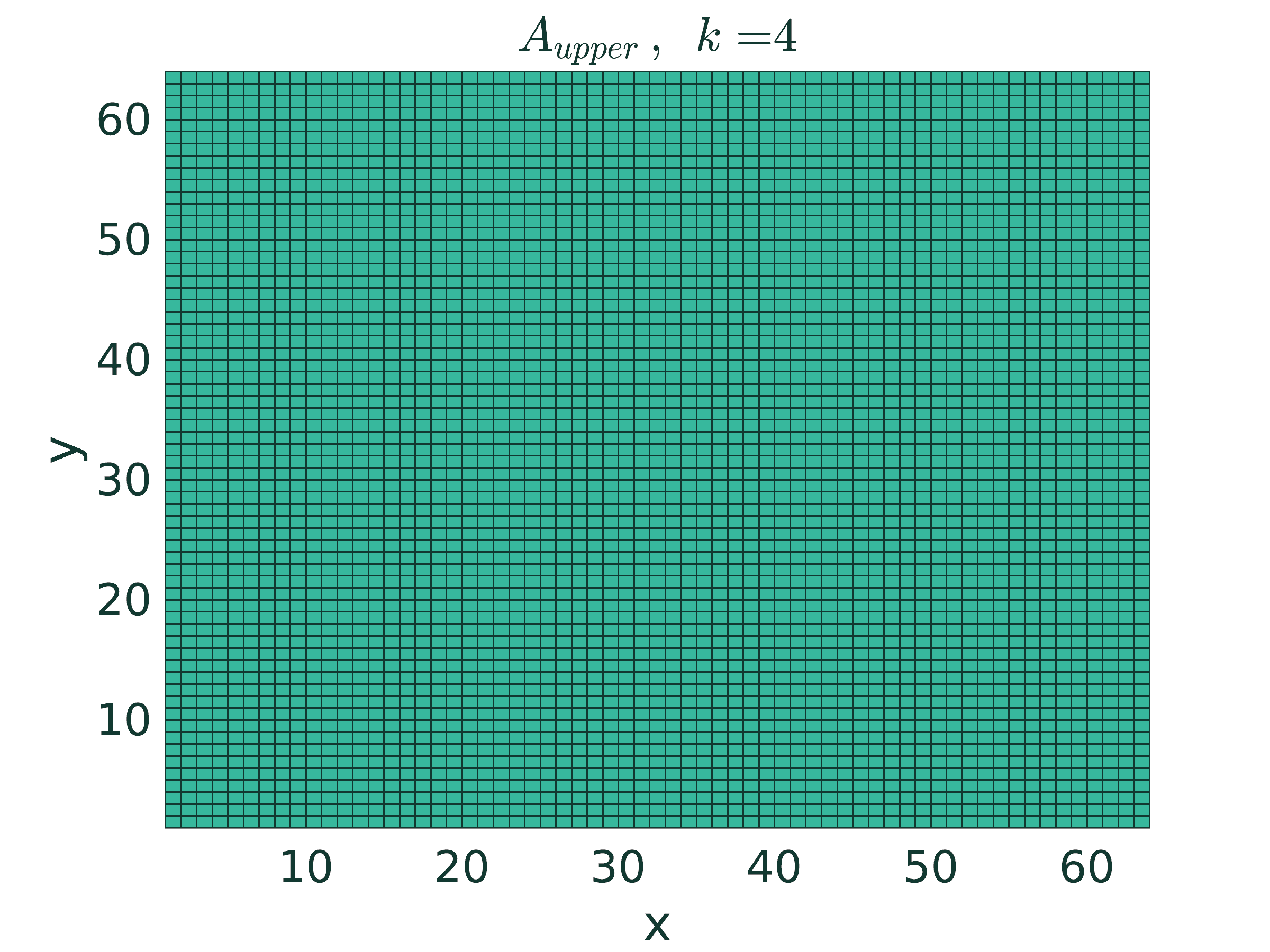
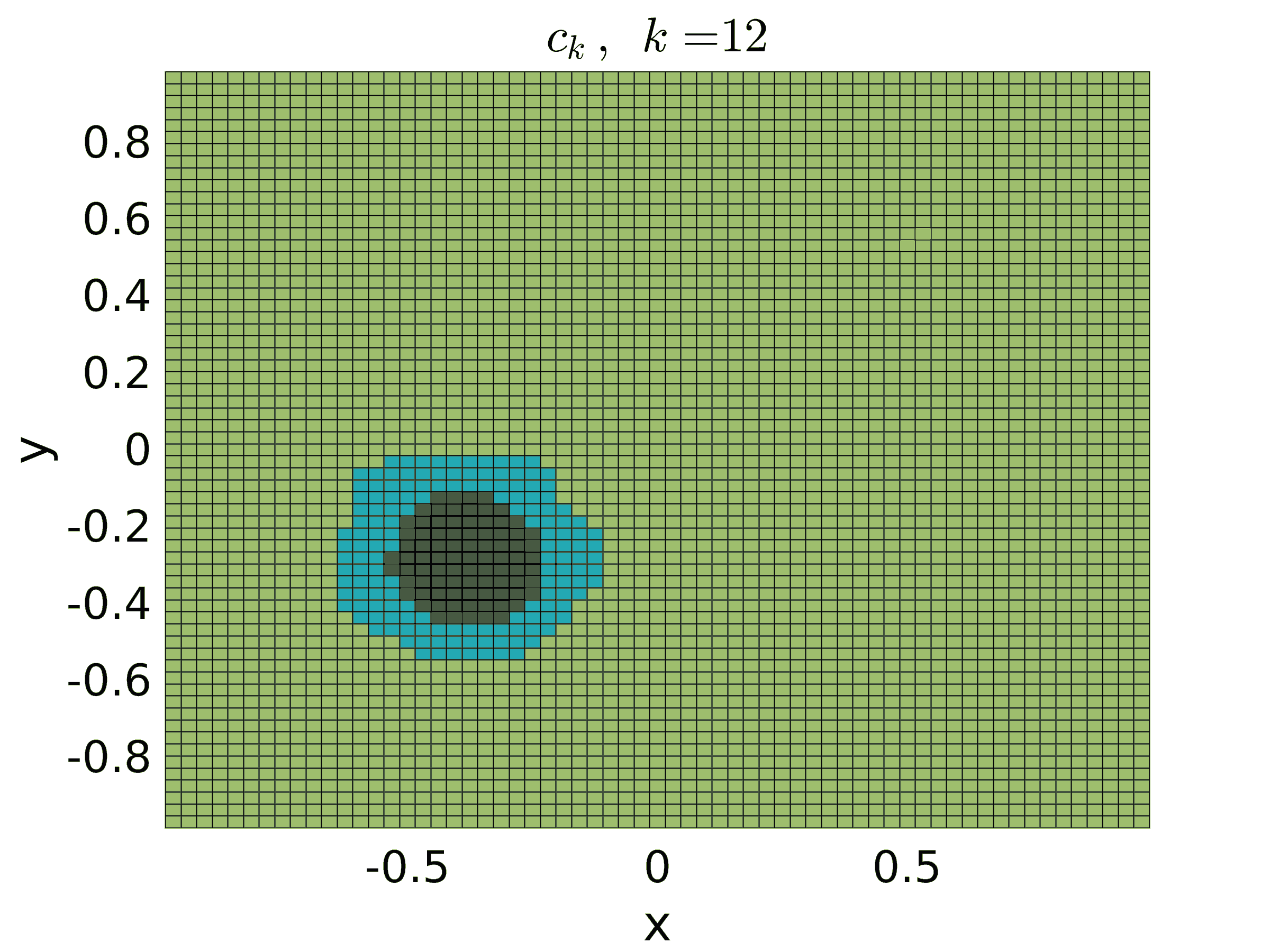
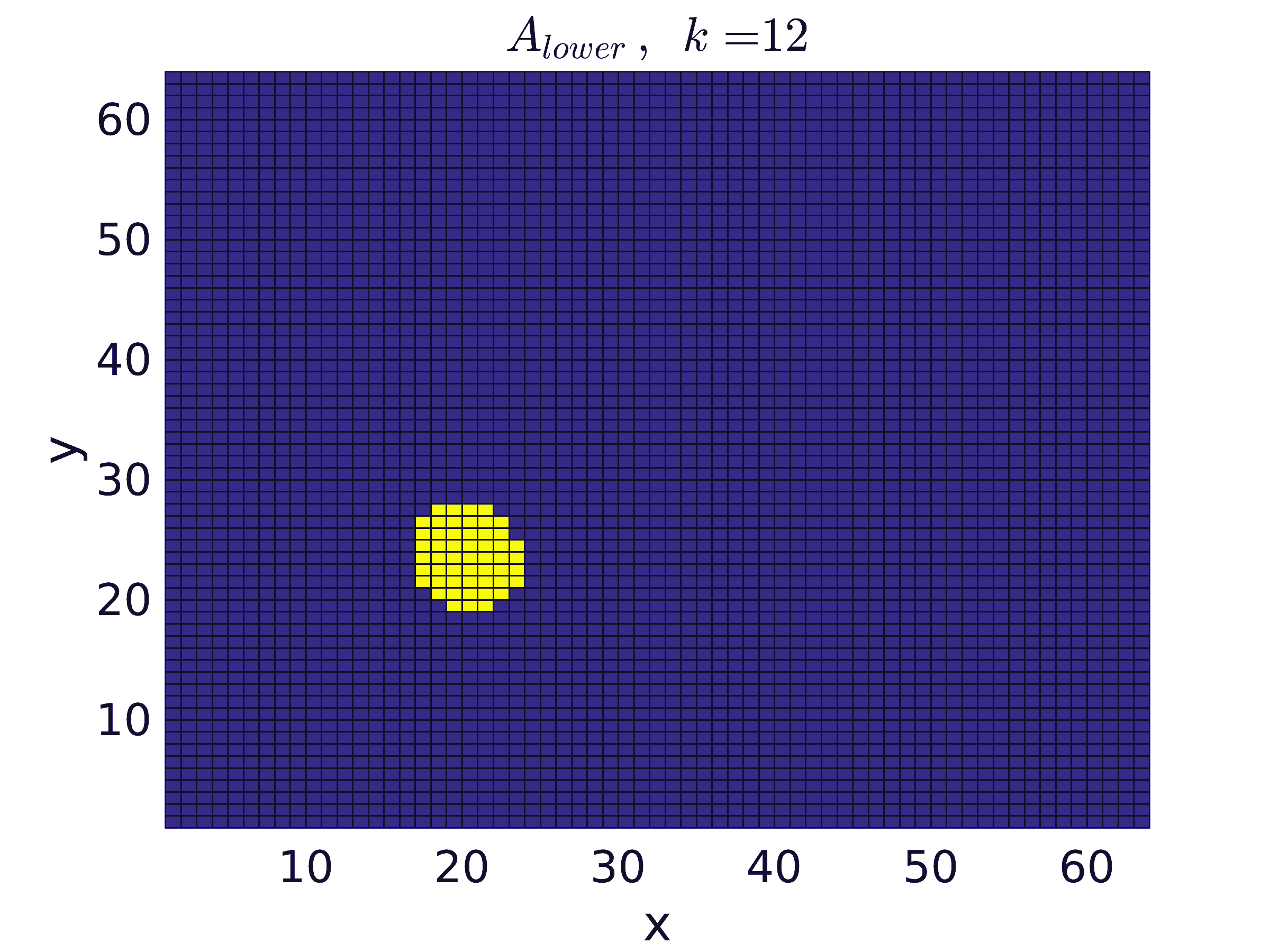
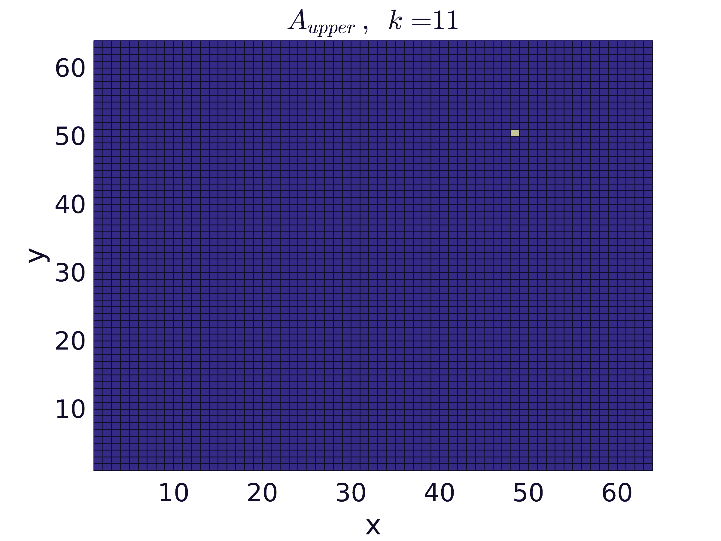
Figure 6: Test 2: Left: reconstructed coefficient $c_{k}$; Middle: active set for lower bound; Right: active set for upper bound; For $k=1,4,8,12$ (top to bottom) and $\delta=0.01$.

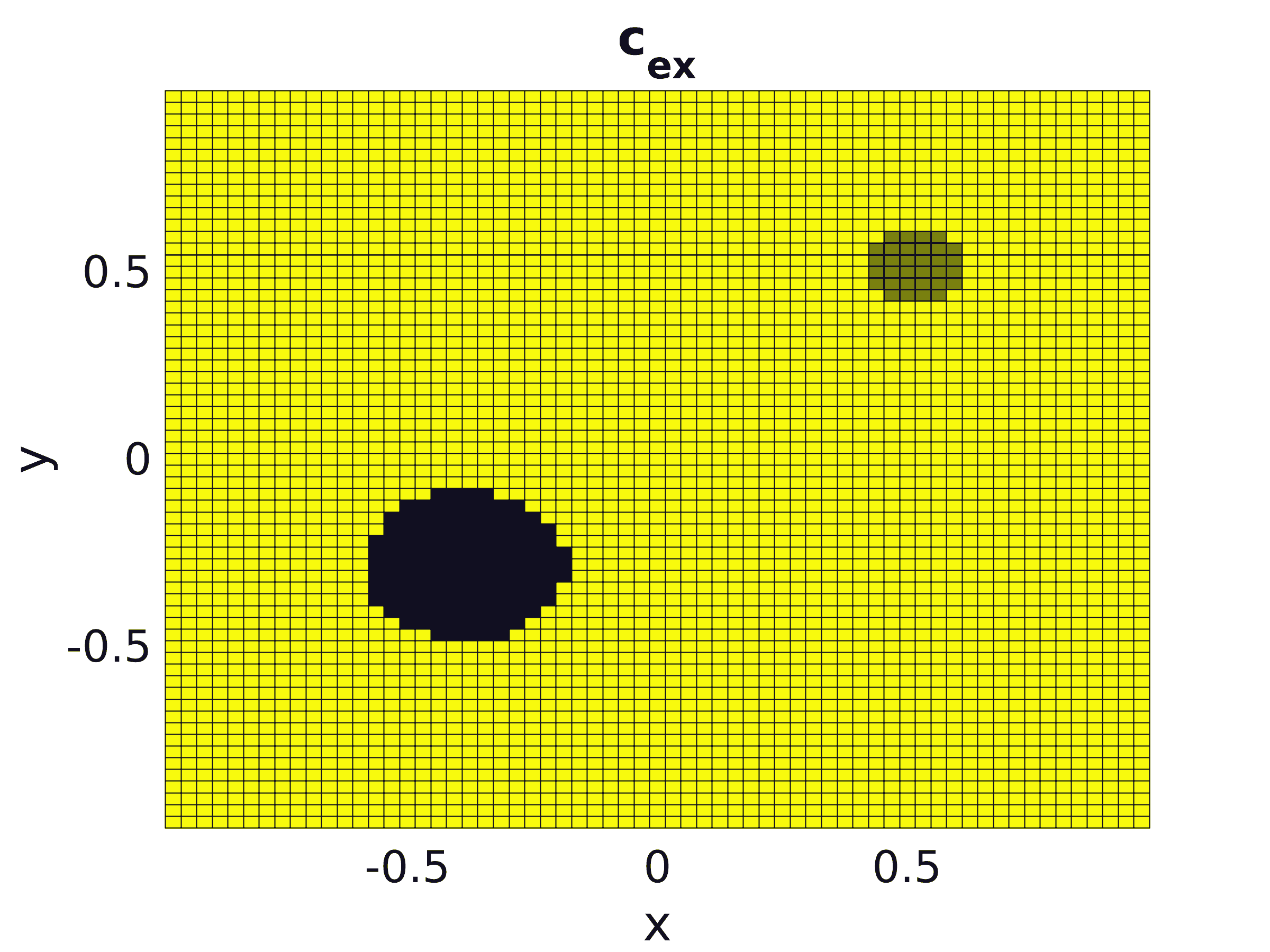
Figure 7: Test 3: left: exact coefficient $c_{ex}$; $\underline{c}=-10$, $\overline{c}=0$; right: locations of spots for testing weak * $L^{\infty}$ convergence

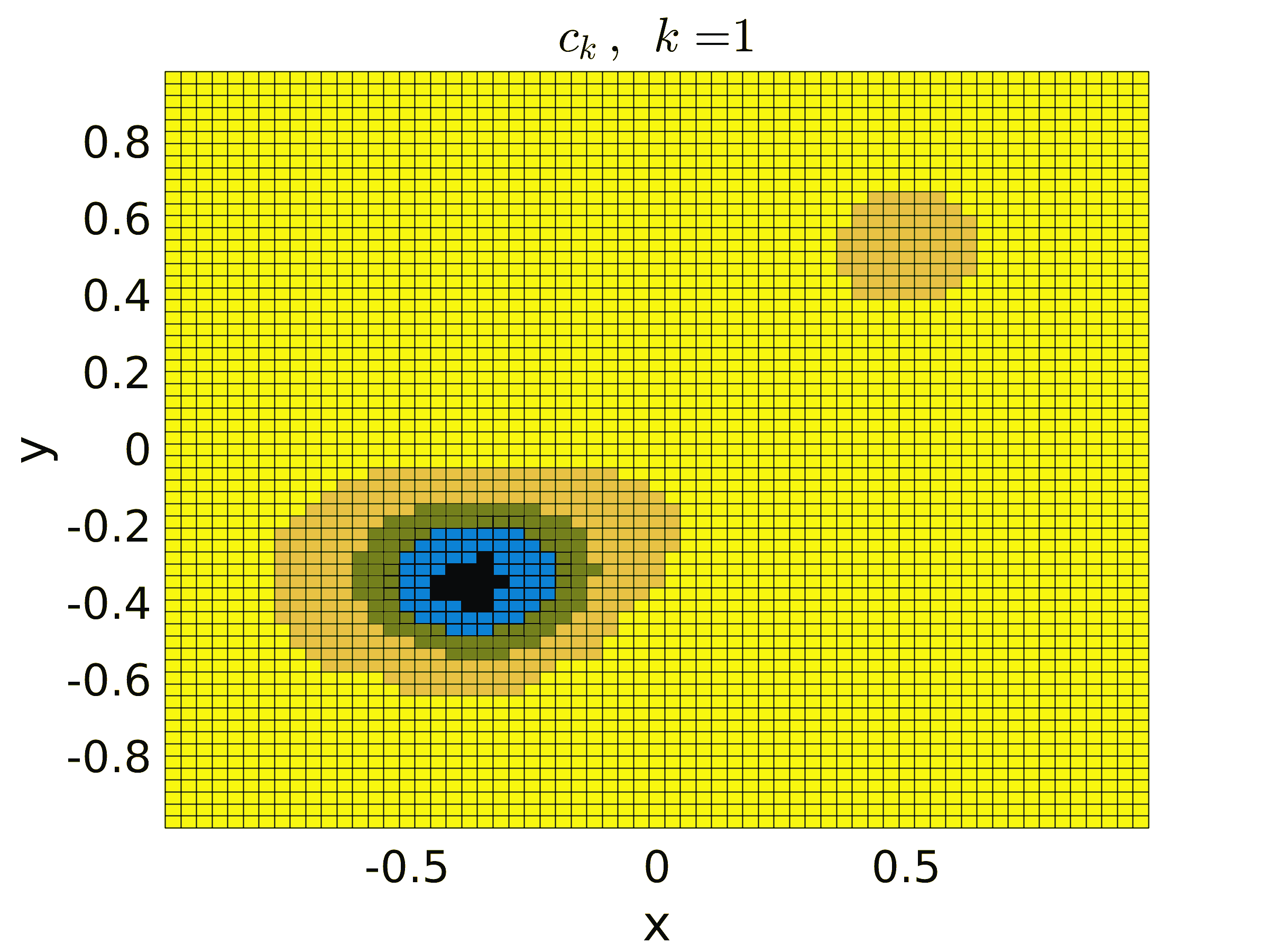
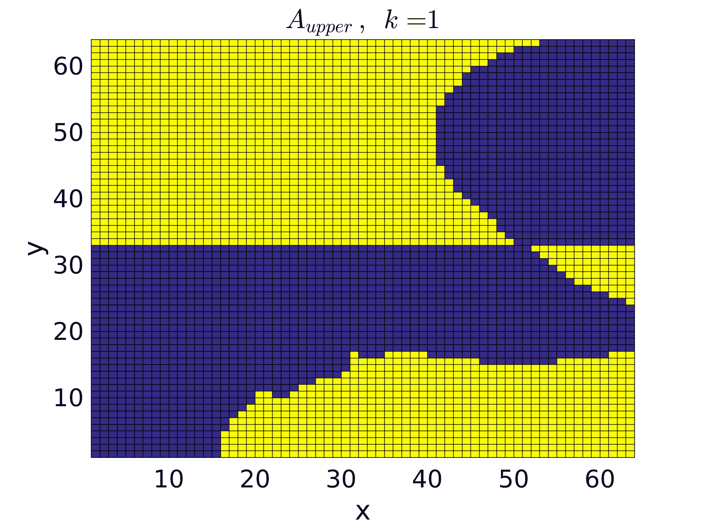
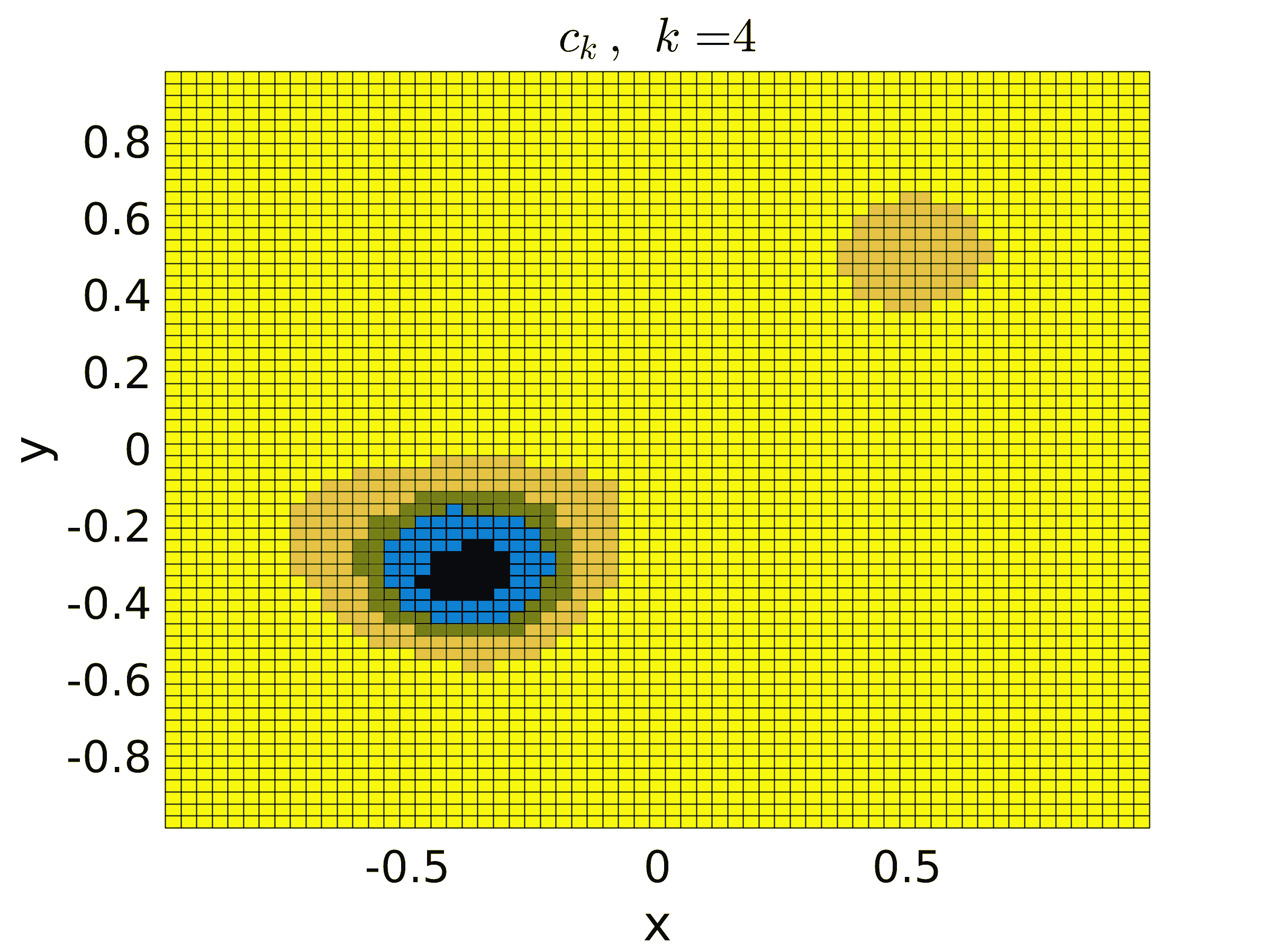
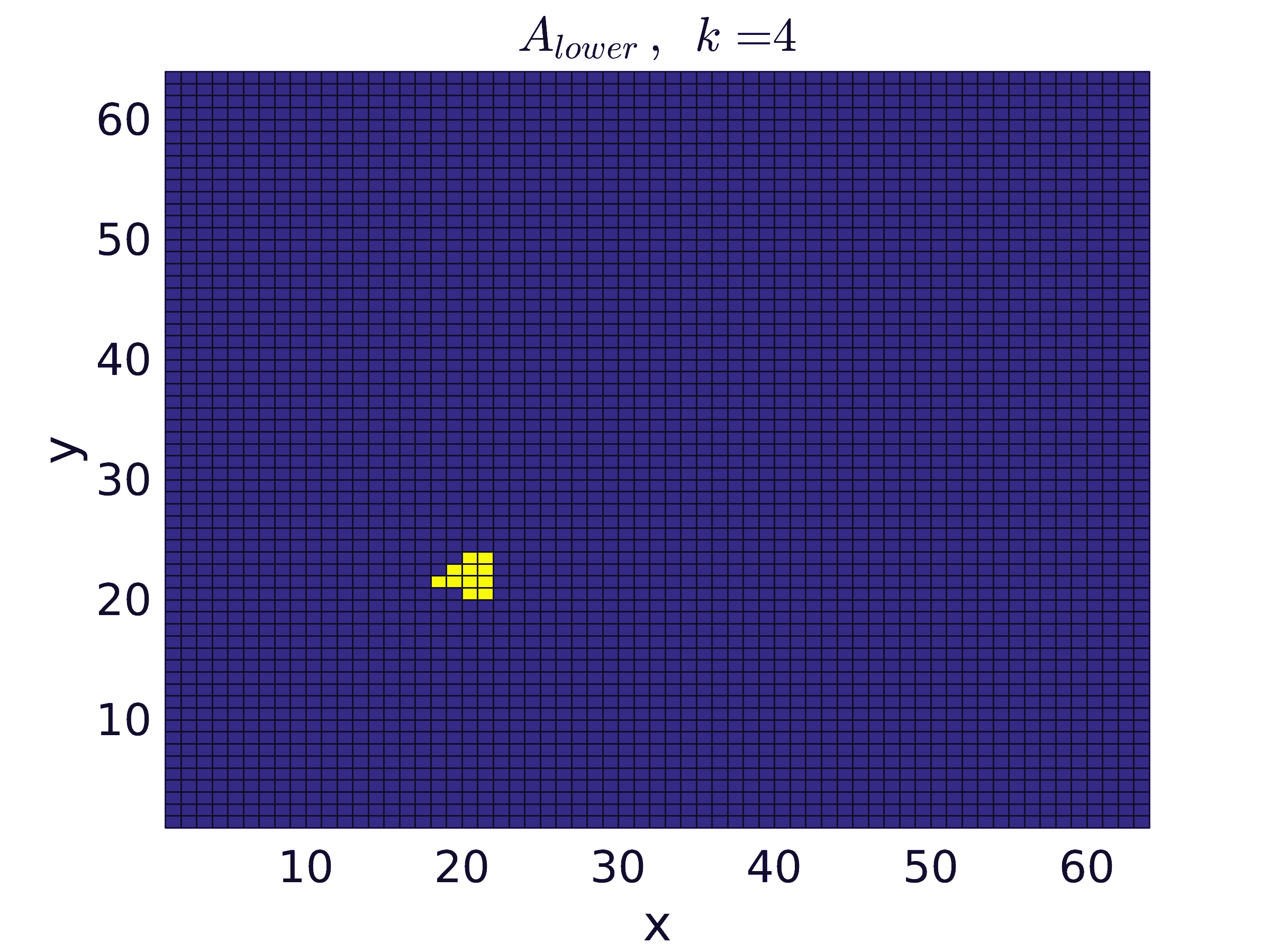
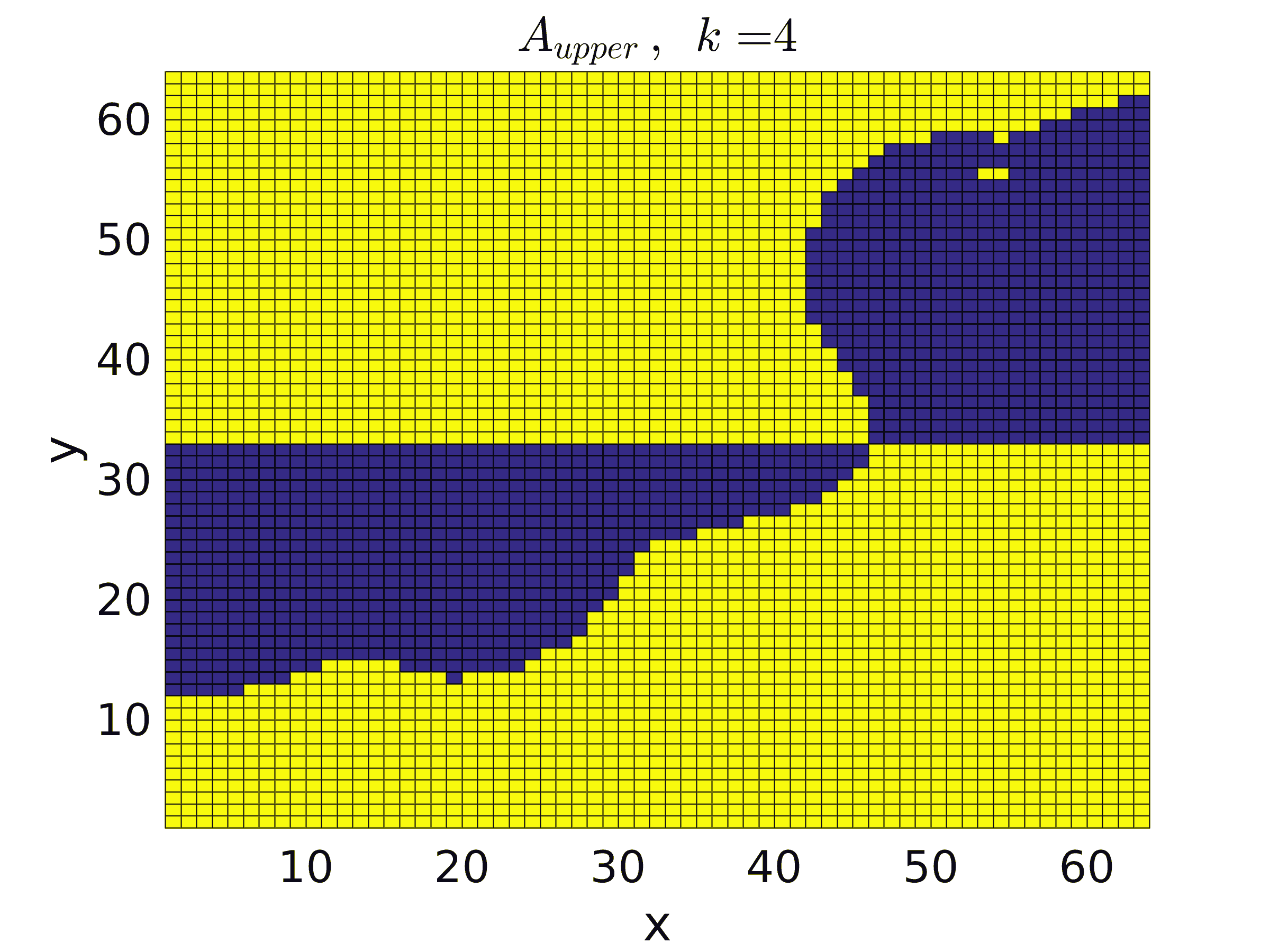
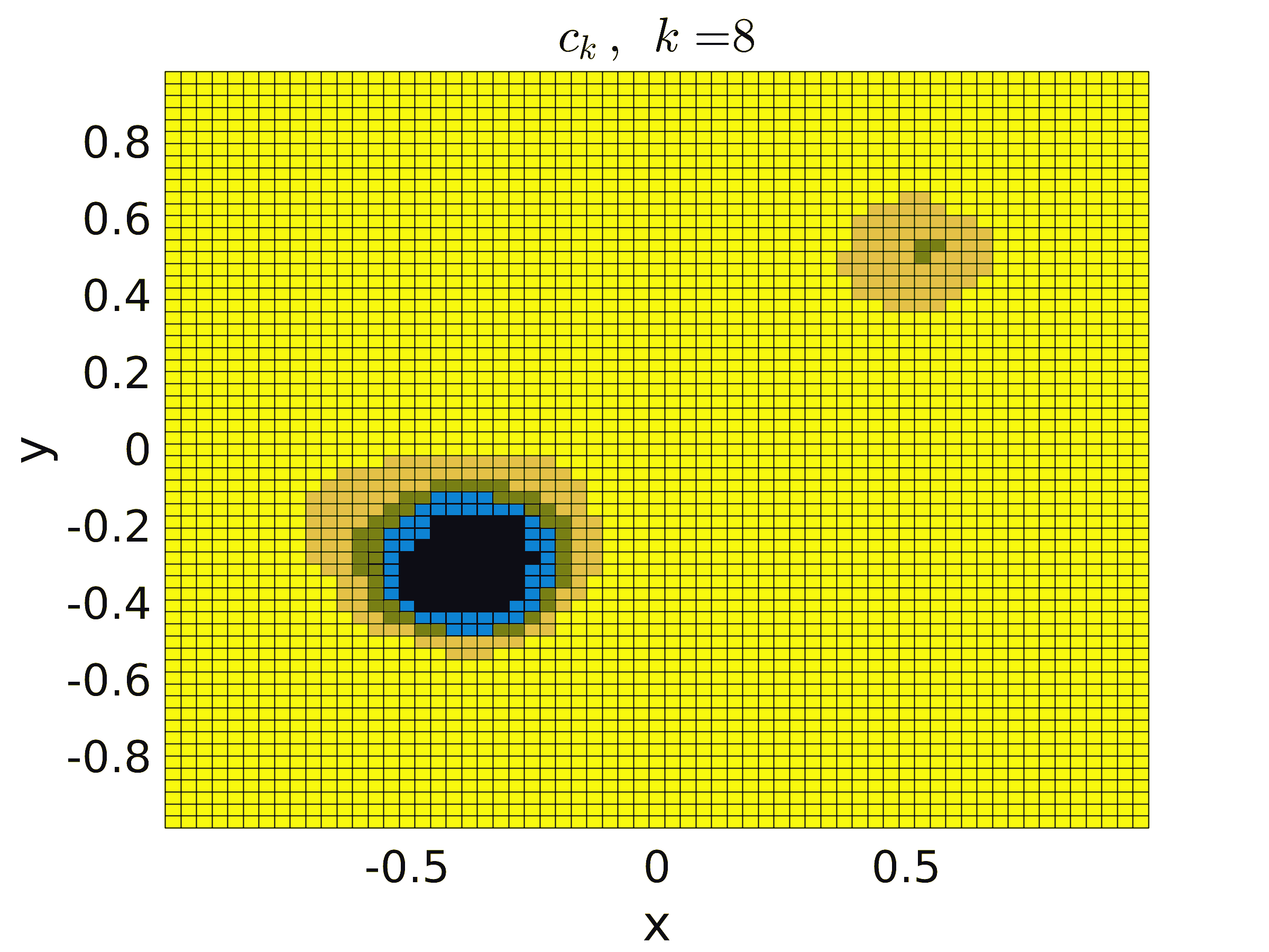
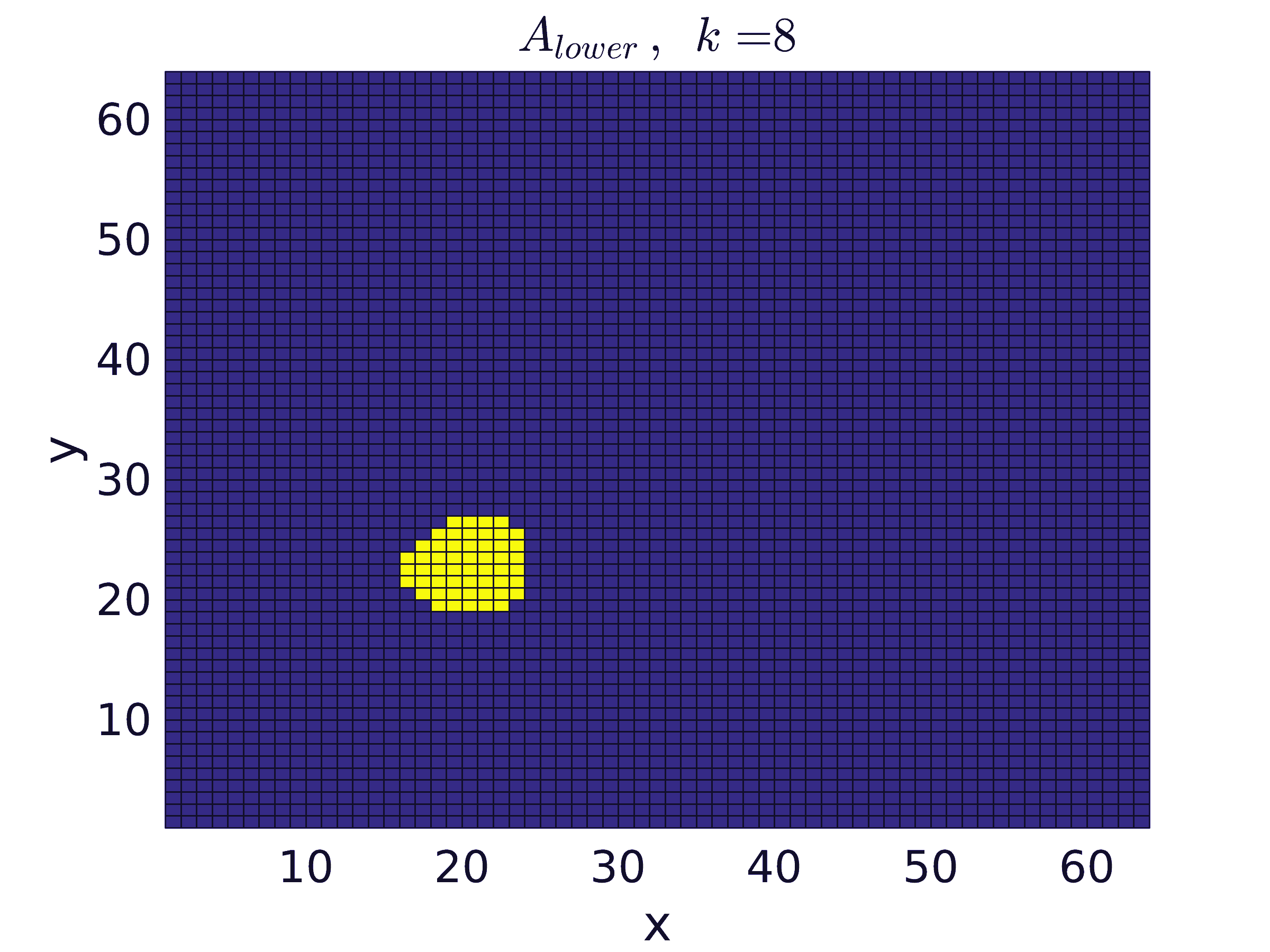
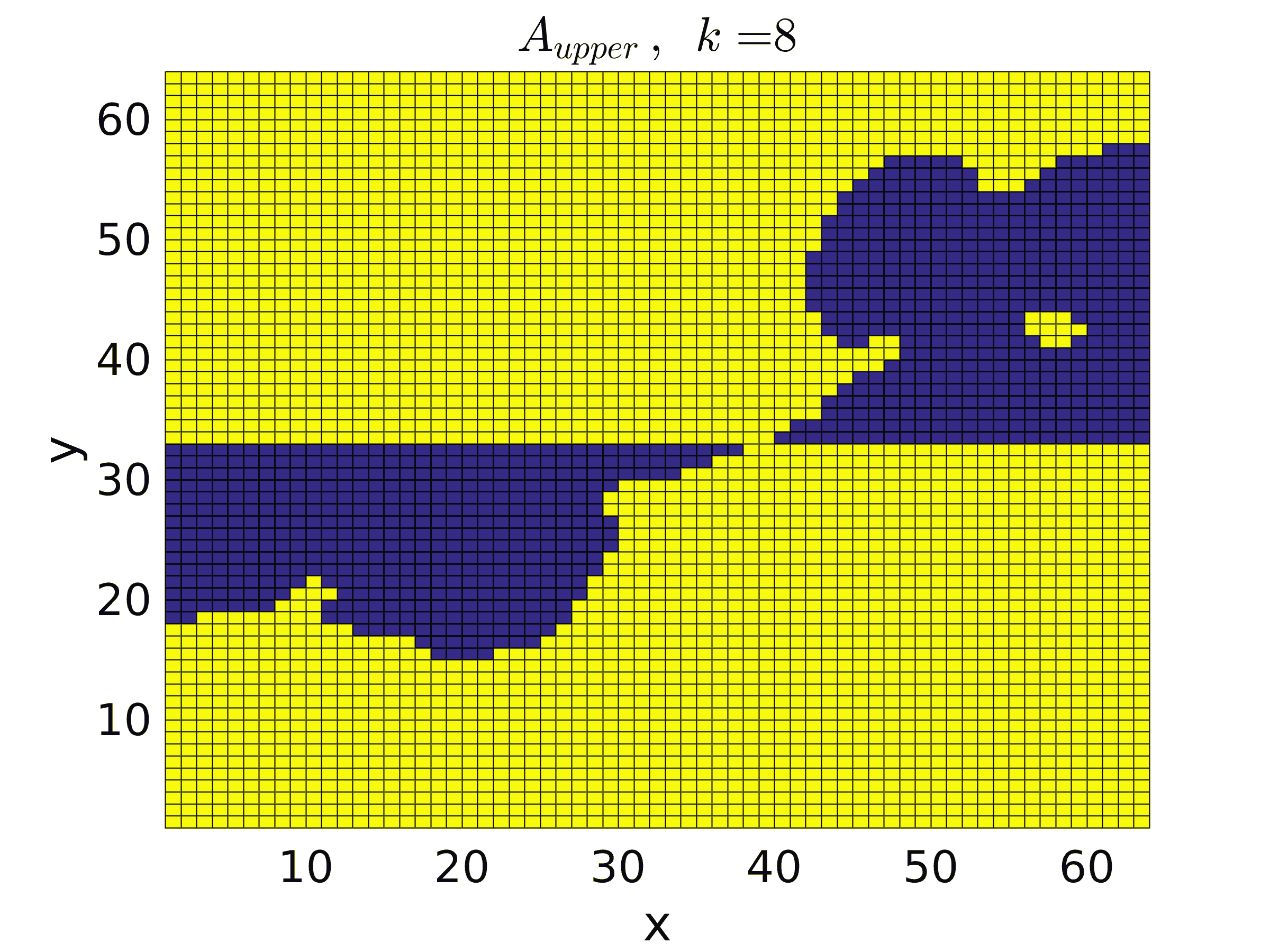
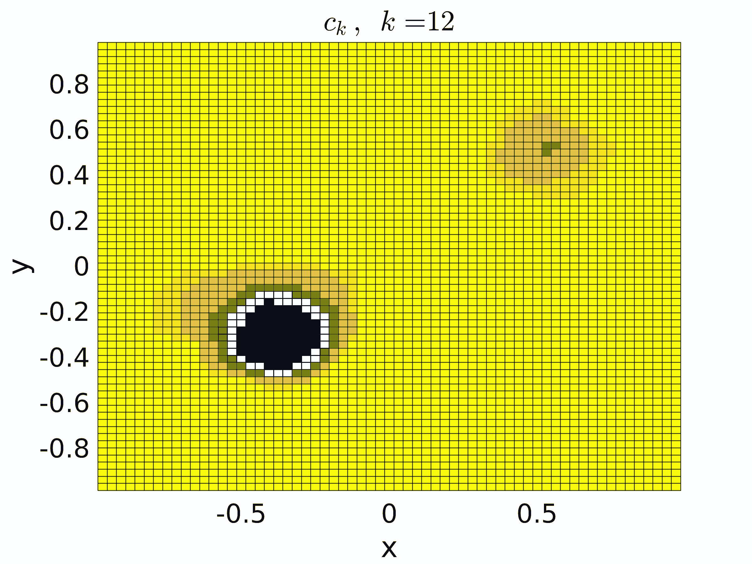
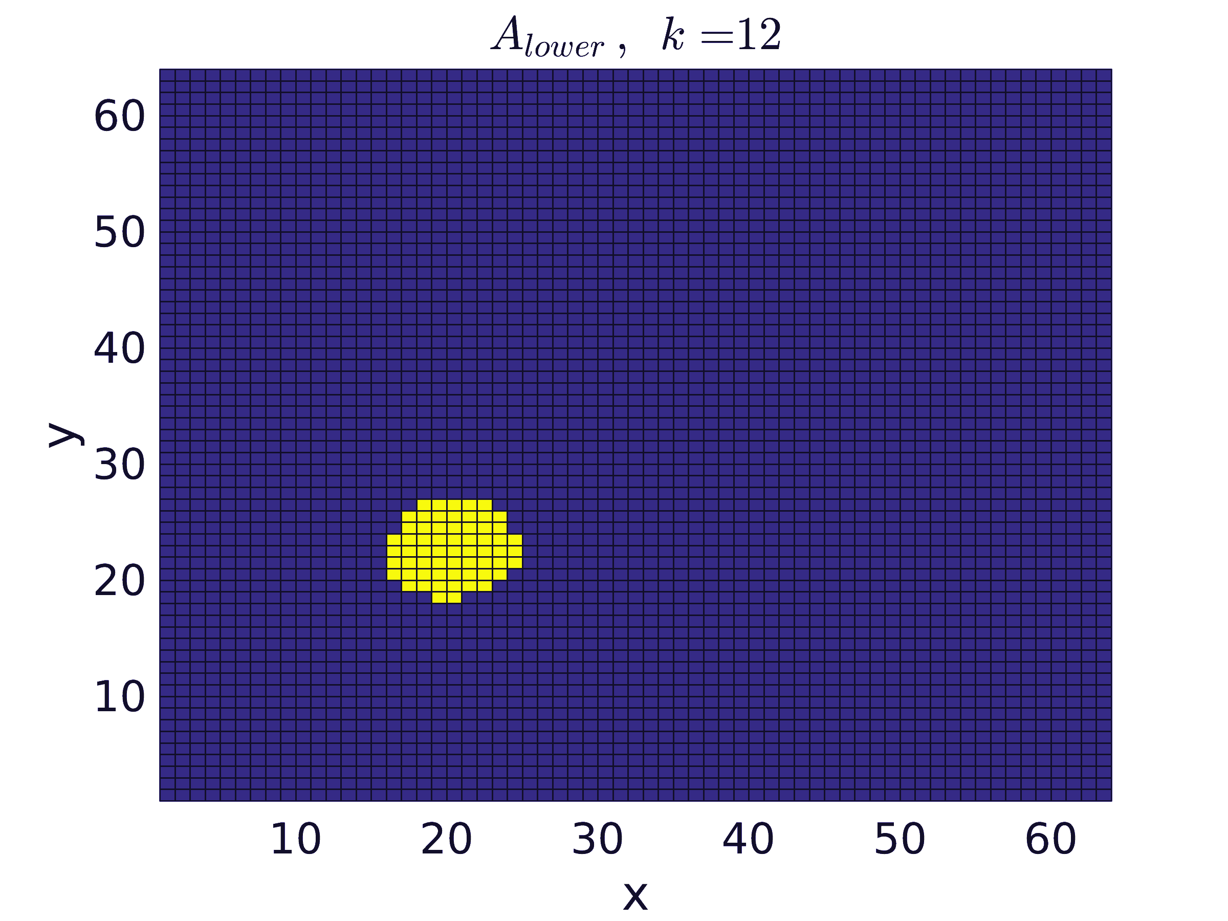
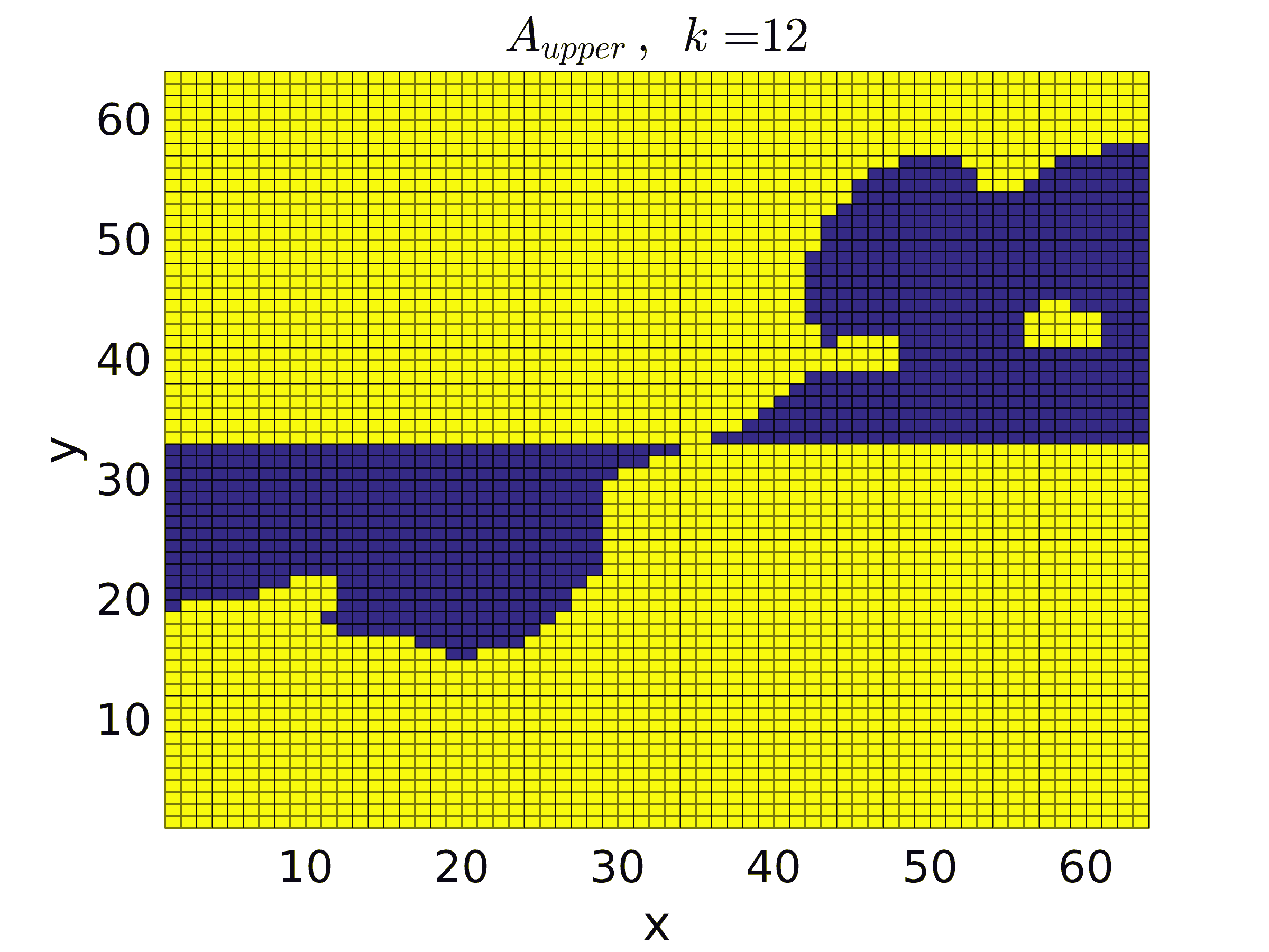
Figure 8: Test 3: Left: reconstructed coefficient $c_{k}$; Middle: active set for lower bound; Right: active set for upper bound; For $k=1,4,8,12$ (top to bottom) and $\delta=0.01$.

7 Conclusions and Remarks

Imposing bounds both on the searched for parameter and on the data misfit is shown to provide an efficient tool for stabilizing inverse problems. The box constrained minimization problems resulting after discretization can be efficiently solved by a Gauss-Newton type SQP approach using recently developed active set methods for box constrained strictly convex quadratic programs. This is demonstrated by three examples of coefficient idenitification in elliptic PDEs.
Future research in this direction might be concerned with strategies dealing with the potential nonconvexity arising due to stronger nonlinearity. (Note that the examples considered here so far can be shown to satisfy the so-called tangential cone condition and are therefore only mildly nonlinear.)
Also investigations on convergence of iterative regularization methods based on formulation (11) in an infinite dimensional function space setting would be of interest. However, this requires to work in nonreflexive spaces both in parameter and in data space, which makes an analysis challenging.

References

• [1] E. Beretta, M. V. de Hoop, F. Faucher and O. Scherzer, Inverse boundary value problem for the Helmholtz equation: quantitative conditional Lipschitz stability estimates, SIAM Journal on Mathematical Analysis 48 (2016), pp. 3962–3983.
• [2] M. Bergounioux, M. Haddou, M. Hintermüller and K. Kunisch, A Comparison of Interior Point Methods and a Moreau-Yosida based Active Set Strategy for Constrained Optimal Control Problems, SIAM Journal on Optimization 11 (2000), pp. 495–521.
• [3] M. Bergounioux and K. Ito and K. Kunisch, Primal-Dual Strategy for Constrained Optimal Control Problems SIAM Journal on Control and Optimization 37 (1999), pp. 1176–1194.
• [4] L. Borcea, Electrical impedance tomography, Inverse Problems 18 (2002) pp. R99–R136.
• [5] T.F. Coleman, and Y. Li, A reflective Newton method for minimizing a quadratic function subject to bounds on some of the variables, SIAM Journal on Optimization 6 (1996), pp. 1040–1058.
• [6] M. Hintermüller and K. Ito and K. Kunisch, The primal-dual active set strategy as a semi-smooth Newton method, SIAM Journal on Optimization 13 (2003), pp. 865–888.
• [7] P. Hungerländer and F. Rendl, A feasible active set method for strictly convex problems with simple bounds, SIAM Journal on Optimization 25 (2015), pp. 1633–1659.
• [8] P. Hungerländer and F. Rendl, An infeasible active set method with combinatorial line search for convex quadratic problems with bound constraints, Journal of Global Optimization (2018), accepted.
• [9] Júdice, Joaquim J. and Pires, Fernanda M., A Block Principal Pivoting Algorithm for Large-scale Strictly Monotone Linear Complementarity Problems, Computers and Operations Research 21 (1994), pp. 587–596.
• [10] B. Kaltenbacher, Minimization based formulations of inverse problems and their regularization, SIAM Journal on Optimization 28 (2018), pp. 620–645.
• [11] S. Kindermann, Convergence of the gradient method for ill-posed problems, Inverse Problems and Imaging (IPI) 4 (2017), pp. 703–720.
• [12] I. Knowles, A variational algorithm for electrical impedance tomography, Inverse Problems 14 (1998), p. 1513.
• [13] Kunisch, K. and Rendl, F., An infeasible active set method for convex problems with simple bounds, SIAM Journal on Optimization 14 (2003), pp. 35–52.
• [14] R. V. Kohn and A. McKenney, Numerical implementation of a variational method for electrical impedance tomography, Inverse Problems, 6 (1990), p. 389.
• [15] R. V. Kohn and M. Vogelius, Relaxation of a variational method for impedance computed tomography, Communications on Pure and Applied Mathematics 40 (1987), pp. 745–777.