Angular distributions in electroweak pion production off nucleons: Odd parity hadron terms, strong relative phases, and model dependence

Abstract

The study of pion production in nuclei is important for signal and background determinations in current and future neutrino oscillation experiments. The first step, however, is to understand the pion production reactions at the free nucleon level. We present an exhaustive study of the charged-current and neutral-current neutrino and antineutrino pion production off nucleons, paying special attention to the angular distributions of the outgoing pion. We show, using general arguments, that parity violation and time-reversal odd correlations in the weak differential cross sections are generated from the interference between different contributions to the hadronic current that are not relatively real. Next, we present a detailed comparison of three, state of the art, microscopic models for electroweak pion production off nucleons, and we also confront their predictions with polarized electron data, as a test of the vector content of these models. We also illustrate the importance of carrying out a comprehensive test at the level of outgoing pion angular distributions, going beyond comparisons done for partially integrated cross sections, where model differences cancel to a certain extent. Finally, we observe that all charged and neutral current distributions show sizable anisotropies, and identify channels for which parity-violating effects are clearly visible. Based on the above results, we conclude that the use of isotropic distributions for the pions in the center of mass of the final pion-nucleon system, as assumed by some of the Monte Carlo event generators, needs to be improved by incorporating the findings of microscopic calculations.

I Introduction

Knowledge of neutrino interaction cross sections is an important and necessary ingredient in any neutrino measurement, and it is crucial for reducing systematic errors affecting present and future neutrino oscillation experiments. This is because neutrinos do not ionize the materials they are passing through, and hence neutrino detectors are based on neutrino-nucleus interactions Morfin et al. (2012); Formaggio and Zeller (2012); Alvarez-Ruso et al. (2014); Katori and Martini (2018); Mosel (2016); Alvarez-Ruso et al. (2018).

The precise determination of neutrino oscillation parameters requires an accurate understanding of the detector responses and this can only be achieved if nuclear effects are under control. Before addressing the nuclear effects, one first needs to fully understand the reaction mechanisms at the hadron level. All this represents a challenge for both hadron and nuclear physics. From a hadron physics perspective, neutrino reactions allow us to investigate the axial structure of the nucleon and baryon resonances, enlarging our knowledge of hadron structure beyond what is presently inferred from experiments with hadronic and electromagnetic probes.

Pion production is one of the main reaction mechanisms for neutrinos with energies of a few GeV Formaggio and Zeller (2012). The MiniBooNE Aguilar-Arevalo et al. (2011) and MINER$\nu$A Eberly et al. (2015); McGivern et al. (2016) collaborations have reported high quality data for weak pion production in the $\Delta(1232)$ region from $CH_{2}$ and $CH$ targets, respectively. Although the best theoretical calculations have been unable to reproduce MiniBooNE data, the models implemented in event generators have been more successful Alvarez-Ruso et al. (2018). All approaches combine pion production off nucleons and pion final state interaction (FSI) models based on the analysis of previous data. The most recent MINER$\nu$A data have features similar to the MiniBooNE data, however, event generators are unable to reproduce simultaneously the magnitude of both data sets.

Some of the differences for pion production cross sections in nuclei found in different approaches have their origin in the differences already existing in the production models used at the free nucleon level. Thus, the first step towards putting neutrino induced pion production on nuclear targets on a firm ground is to have a realistic model at the nucleon level. From this perspective, in this work we make an exhaustive study of charged current (CC) and neutral current (NC) neutrino and antineutrino pion production reactions off nucleons, paying special attention to the angular distributions of the outgoing pion. We show, using general arguments, that the possible dependencies on the azimuthal angle ($\phi^{*}_{\pi}$) measured in the final pion-nucleon center of mass (CM) system are $1,\cos\phi^{*}_{\pi},\cos 2\phi^{*}_{\pi},\sin\phi^{*}_{\pi}$ and $\sin 2\phi^{*}_{\pi}$, and that the two latter ones give rise to parity violation and time-reversal odd correlations in the weak differential cross sections, as already found in Refs. Hernández et al. (2007a, b). Here, we make a detailed discussion of the origin of the parity-violating contributions, and explicitly show that they are generated from the interference between different contributions to the hadronic current that are not relatively real. Next, we present a detailed comparison of three, state of the art, microscopic models for electroweak pion production off nucleons. One is the dynamical coupled-channel model (DCC) developed at Argonne National Laboratory (ANL) and Osaka University Matsuyama et al. (2007); Kamano et al. (2013); Nakamura et al. (2015). This approach provides a unified treatment of all resonance production processes. It satisfies unitarity and its predictions have been extensively and successfully compared to data on $\pi N$ and $\gamma N$ reactions up to invariant masses slightly above 2 GeV. The second model included in this comparison is the one initiated by T. Sato and T.S.H. Lee (SL) to describe pion production by photons and electrons Sato and Lee (1996, 2001) and also by neutrinos Sato et al. (2003); Matsui et al. (2005); Sato and Lee (2009), in the $\Delta(1232)$ region. In fact, one can consider the DCC model as an extension of the SL model to higher $\pi N$ invariant masses. The last model we consider was initially developed by E. Hernández, J. Nieves and M. Valverde (HNV) in Ref. Hernández et al. (2007a), and it is based on the approximate chiral symmetry of QCD. The model was later improved in Refs. Hernández et al. (2013); Alvarez-Ruso et al. (2016); Hernández and Nieves (2017), incorporating among other effects a partial restoration of unitarity, through the implementation of Watson theorem in the $P_{33}$ pion-nucleon channel. A brief description of these models will be given below, while further details can be consulted in the above given references.

Though in this work we are mainly interested in neutrino induced reactions, we shall dedicate a full section to pion electroproduction. In this way, we can make a direct comparison of the vector part of the different models and data. Since the quality of the data is very good in this case, we can use this comparison to extract relevant information on the vector part of the models. We will show that the bulk of the DCC model predictions for electroproduction of pions in the $\Delta$ region could be reproduced, with a reasonable accuracy, by the simpler HNV model. Given the high degree of complexity and sophistication of the DCC approach, we find that this validation is remarkable. The HNV model might be more easily implemented in the Monte Carlo event generators used for neutrino oscillation analyses, and this would contribute to a better theoretical control of such analyses.

Furthermore, we show that the DCC and HNV models agree reasonably well for CC and NC neutrino and antineutrino total cross sections, as well as for the corresponding differential cross sections with respect to the outgoing lepton variables. With respect to the pion angular dependence of the weak cross sections, we will observe, first of all, that CC and NC distributions show clear anisotropies. This means that using an isotropic distribution for the pions in the CM of the final pion-nucleon system, as assumed by some of the Monte Carlo event generators, is not supported by the results of the DCC and HNV models. We will also illustrate the importance of carrying out a comprehensive test of the different models at the level of outgoing pion angular distributions, going beyond comparisons done for partially integrated cross sections, where model differences tend to cancel. Finally, we will discuss the pion azimuthal angular distributions, where parity violation shows up mainly through the $\sin\phi^{*}_{\pi}$ term mentioned above and discussed in detail in what follows. We will show that parity violation is quite significant for NC neutrino reactions producing charged pions, and especially for the $\nu_{e}n\to e^{-}n\pi^{+}$ and $\bar{\nu}_{e}p\to e^{+}p\pi^{-}$ CC processes, where background non-resonant contributions are sizable. The azimuthal distributions for these weak processes could provide information on the relative phases of different hadronic current contributions that would be complementary to that inferred from polarized electron scattering.

The work is organized as follows: In Sec. II, we give a brief description of the DCC and HNV models. In Sec. III we discuss different expressions for neutrino induced pion production differential cross sections. One of them makes explicit the dependence on the pion azimuthal angle, which is easily related to the violation of parity. Next, we discuss how parity violation originates from the interference of different contributions to the hadronic current that are not relatively real. In Sec. IV, we present an extensive collection of results for total and differential cross sections for pion production by neutrinos and antineutrinos. Sec. V is dedicated to pion electroproduction. Finally in Sec. VI we present an exhaustive summary of this study. In addition, we include four appendixes. In Appendix A, we give the Lorentz transformation from the laboratory system to the CM of the final pion-nucleon, paying special attention to the form of the different four-vectors in the latter system. In Appendix B, we compile some auxiliary equations that help determine the dependence on the pion azimuthal angle of the electro-weak pion production off the nucleon. In Appendix C, we give the CC differential cross section for pion production by neutrinos as a sum over cross sections for virtual $W$ of different polarization. For that purpose, we introduce and evaluate the helicity components of the lepton and hadron tensors. The final expression, evaluated for massless leptons, is analogous to the corresponding one commonly used for pion electroproduction, which is rederived in Appendix D.

II Brief description of the DCC and HNV models

II.1 DCC model

The DCC model Matsuyama et al. (2007); Kamano et al. (2013) was designed to describe meson-baryon scattering and electroweak meson production in the nucleon resonance region in a unified manner. To describe the hadron states up to invariant masses $W\ \raise 1.29167pt\hbox{$<$\kern-7.5pt\lower 4.30554pt\hbox{$\sim$}}\ 2$ GeV, the model includes stable two-particle channels $\pi N,\eta N,K\Lambda,K\Sigma$ and unstable particle channels $\rho N,\sigma N,\pi\Delta$, the latter being the doorway states to the three-body $\pi\pi N$ state. The $T$-matrix for the meson-baryon scattering is obtained by solving the coupled-channel Lippmann-Schwinger equation,

$$\langle\alpha,\vec{p}\,^{\prime}|T(W)|\beta,\vec{p}\,\rangle = \langle\alpha,\vec{p}\,^{\prime}|V(W)|\beta,\vec{p}\,\rangle+\sum_{\gamma}\int d^{3}{k}\,\langle\alpha,\vec{p}\,^{\prime}|V(W)|\gamma,\vec{k}\,\rangle G_{\gamma}^{0}(\vec{k},W)\langle\gamma,\vec{k}\,|T(W)|\beta,\vec{p}\,\rangle,$$ (1)

where $\alpha,\beta$ and $\gamma$ denote meson-baryon two-body states and $\vec{p}$ etc., the three-momenta in their CM. The energy ($W$) dependent effective potential is split into three contributions ,

$$V(W)=v_{\rm non-res}+\Gamma\frac{1}{W-m^{0}_{\rm res}}\Gamma^{\dagger}+Z(W)\ .$$ (2)

The $v_{\rm non-res}$ term consists of non-resonant meson-baryon interactions that include $t$-channel meson exchange and $u$-, and $s$-channel baryon exchange mechanisms. The second term includes bare $N^{*}$ and $\Delta$ excitation $s$-channel processes, with $m^{0}_{\rm res}$ and $\Gamma$ the bare mass and bare decay vertex of an unstable resonance . The last term $Z(W)$ is a particle-exchange diagram including $\pi\pi N$ intermediate states. The Green function $G_{\gamma}^{0}(\vec{k},W)$ is the meson($M_{\gamma}$)-baryon($B_{\gamma}$) propagator for a channel $\gamma$ and is written as

$$G_{\gamma}^{0}(\vec{k},W) = \frac{1}{W-[E_{B_{\gamma}}(\vec{k}\,)+E_{M_{\gamma}}(\vec{k}\,)+\Sigma_{\gamma}(\vec{k},W)]+i\epsilon}\ .$$ (3)

The decay of an unstable particle channel into $\pi\pi N$ is included in $\Sigma_{\gamma}(\vec{k},W)$. By considering $Z(W)$ and $\Sigma_{\gamma}$, the $T$-matrix satisfies not only two-body unitarity but also three-body unitarity Matsuyama et al. (2007).

The electroweak meson production amplitudes from the DCC model are given as

$$\langle\alpha,\vec{p}\,^{\prime}|J^{\mu}(q)|N(\vec{p}\,)\rangle = \langle\alpha,\vec{p}\,^{\prime}|j^{\mu}(q)|N(\vec{p}\,)\rangle+\sum_{\gamma}\int d^{3}{k}\,\langle\alpha,\vec{p}\,^{\prime}|T(W)|\gamma,\vec{k}\,\rangle G_{\gamma}^{0}(\vec{k},W)\langle\gamma,\vec{k}\,|j^{\mu}(q)|N(\vec{p}\,)\rangle,$$ (4)

where the electroweak meson production current ($j^{\mu}$) consists of a non-resonant meson production current $j^{\mu}_{\rm non-res}$ including $s$-, $t$- and $u$-channel exchange mechanisms similar to $v_{\rm non-res}$, and a nucleon resonance excitation contribution:

$$j^{\mu}=j^{\mu}_{\rm non-res}+\Gamma\frac{1}{W-m^{0}_{\rm res}}\Gamma^{\mu}\ .$$ (5)

One of the present authors, T.S., initiated a development of a dynamical approach, referred in this work as the SL model, with the aim of providing a reasonable description of $\pi N$ scattering and electroweak pion production in the $\Delta(1232)$ region in a unified manner Sato and Lee (1996, 2001); Sato et al. (2003); Matsui et al. (2005); Sato and Lee (2009). The aim of the SL model was to study the electroweak pion production of the $\Delta(1232)$ resonance. Therefore, the only meson-baryon channel included is the $\pi N$ state and the model cannot be applied beyond the $\Delta(1232)$ resonance region. The DCC approach described in the above paragraph can be viewed as an extension of the SL model to a higher resonance region, and it has been developed through the analysis of the large available data sample on differential cross sections and polarization observables for pion- and photo-induced meson production reactions ($\sim$23,000 data points). The resonance masses, widths, and electromagnetic couplings for $N\to N^{*},\Delta$ transitions have been extracted from the partial wave amplitudes of the model at the pole positions. The DCC approach was extended to describe the neutrino-induced meson production reactions in Refs. Nakamura et al. (2015, 2017). The vector current at finite $q^{2}$ (four-momentum transfer square) and the isovector couplings of the isospin 1/2 resonances are determined by analyzing data for pion electroproduction and the photo reaction on the neutron. The axial couplings for the $N\to N^{*},\Delta$ transitions are determined by the pion coupling constants, assuming partial conservation of the axial current (PCAC), while dipole $q^{2}$-dependence is assumed for the axial form factors. In this work, we use a 10% weakened bare axial coupling constant , $g_{AN\Delta}({\rm new})=0.9\,g_{AN\Delta}({\rm original})$, for the $N\to\Delta(1232)$ transition, as compared to the value used in Nakamura et al. (2015, 2017). While $g_{AN\Delta}({\rm original})$ was obtained using PCAC, $g_{AN\Delta}({\rm new})$ is chosen so as to give a better reproduction of the neutrino cross section data of Ref. Rodrigues et al. (2016) that have been obtained from a reanalysis of old ANL and Brookhaven National Laboratory (BNL) data.

II.2 HNV model

The HNV model was originally introduced in Ref. Hernández et al. (2007a) to describe pion production by neutrinos in the $\Delta$ resonance region. In its first version, it included the dominant direct and crossed $\Delta-$pole terms plus a set of background terms. The weak $N\to\Delta$ transition matrix element was parametrized in terms of four vector $C^{V}_{3-6}$ and four axial $C^{A}_{3-6}$ form factors. Vector form factors were known from the study of pion electroproduction (in fact $C_{6}^{V}$ was set exactly to zero from conservation of the vector current (CVC) ), while axial form factors were mostly unknown. The term proportional to $C_{5}^{A}$ gives the dominant contribution. Assuming the pion pole dominance of the pseudoscalar $C_{6}^{A}$ form factor, the PCAC hypothesis gives $C_{6}^{A}$ in terms of $C_{5}^{A}$. In the absence of good experimental data that allowed for an independent determination of all axial form factors, Adler’s model Adler (1968), in which $C^{A}_{3}=0$ and $C^{A}_{4}=-\frac{1}{4}C_{5}^{A}$, was adopted. Thus, $C_{5}^{A}$ remained as the only unknown form-factor and its value at $q^{2}=0$ and its $q^{2}$ dependence were fitted to experiment.

The background terms are required and fixed by chiral symmetry and they were obtained from the leading order predictions of a SU(2) nonlinear sigma model. The weak vertexes were supplemented with well established form factors in a way that preserved CVC and PCAC. The Feynman diagrams for the different contributions to $W^{+}N\to N^{\prime}\pi$ (corresponding to a CC process induced by neutrinos) are depicted in Fig. 1. All sort of details can be found in Ref. Hernández et al. (2007a). NC pion production by neutrinos as well as antineutrino induced processes were also discussed in Hernández et al. (2007a). NC amplitudes were also given in terms of the resonant and background contributions introduced above, though in this case nucleon strange form-factors needed to be considered. Some preliminary results were also shown in Ref. Hernández et al. (2007b), where NC neutrino and antineutrino pion production reactions were suggested as a way to distinguish $\nu_{\tau}-$neutrinos from antineutrinos, below the $\tau-$production threshold, but above the pion production one.

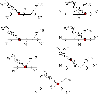
Figure 1: Model for the $W^{+}N\to N^{\prime}\pi$ reaction as introduced in Ref. Hernández et al. (2007a). It contains the Delta ($\Delta P$) and crossed Delta pole ($C\Delta P$) terms (first row), the nucleon ($NP$) and crossed nucleon pole ($CNP$) terms (second row), the contact $CT$ and pion pole ($PP$) terms (third row), and the pion in flight ($PF$) term (fourth row).

To extend the HNV model to neutrino energies up to 2 GeV, in Ref. Hernández et al. (2013), the authors included the two contributions depicted in Fig. 2, which are driven by the exchange of the spin-3/2 $D_{13}(1520)$ resonance.

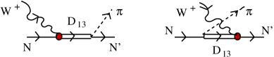
Figure 2: $D_{13}(1520)$ contributions to $W^{+}N\to N^{\prime}\pi$ introduced in Ref. Hernández et al. (2013). Both $D_{13}$ ($DP$) and crossed $D_{13}$ pole ($CDP$) terms are considered.

According to Ref. Leitner et al. (2009), this is the only extra resonance giving a significant contribution in that neutrino energy region. All the details concerning the $DP$ and $CDP$ contributions can be reviewed in the Appendix of Ref. Hernández et al. (2013).

In Ref. Alvarez-Ruso et al. (2016) the HNV model was partially unitarized by imposing Watson theorem. Watson theorem is a consequence of unitarity and time reversal invariance. It implies that, below the two-pion production threshold, the phase of the electro or weak pion production amplitude should be given by the $\pi N\to\pi N$ elastic phase shifts $\left[\delta_{L_{2J+1,2T+1}}(W_{\pi N})\right]$, with $W_{\pi N}$ the final $\pi N$ invariant mass. The procedure followed in Ref. Alvarez-Ruso et al. (2016) was inspired by that implemented by M.G. Olsson in Ref. Olsson (1974). To correct the interference between the dominant $\Delta P$ term and the background (including here not only the nonresonant background, but also the $C\Delta P$, $DP$ and $CDP$ terms), the authors introduced two independent vector and axial phases, that are functions of $q^{2}$ and $W_{\pi N}$. The amplitude was changed as

$$T_{B}+T_{\Delta P}\to T_{B}+e^{i\delta_{V}}T^{V}_{\Delta P}+e^{i\delta_{A}}T^{A}_{\Delta P}$$ (6)

where the vector $\delta_{V}$ and axial $\delta_{A}$ Olsson phases were fixed by requiring that the dominant vector and axial multipoles with the $\Delta(1232)$ quantum numbers have the correct phase $\delta_{P_{33}}(W_{\pi N})$. See Ref. Alvarez-Ruso et al. (2016) for details.

Very recently Hernández and Nieves (2017), the HNV model has been supplemented with additional local terms. The aim was to improve the description of the $\nu_{\mu}n\to\mu^{-}n\pi^{+}$ channel, for which most theoretical models give predictions much below experimental data. As discussed in Ref. Hernández and Nieves (2017), this channel gets a large contribution from the $C\Delta P$ term and then it is sensitive to the spin 1/2 component of the Rarita Schwinger (RS) covariant $\Delta$ propagator. Starting from the case of zero width, the $\Delta$ propagator was modified in that reference as

$$\frac{P_{\mu\nu}(p_{\Delta})}{p_{\Delta}^{2}-M_{\Delta}^{2}} \to \frac{P_{\mu\nu}(p_{\Delta})+c\left(P_{\mu\nu}(p_{\Delta})-\frac{p^{2}_{\Delta}}{M_{\Delta}^{2}}P_{\mu\nu}^{\frac{3}{2}}(p_{\Delta})\right)}{p_{\Delta}^{2}-M_{\Delta}^{2}}$$ (7)

$$= \frac{P_{\mu\nu}(p_{\Delta})+c(p_{\Delta}^{2}-M_{\Delta}^{2})\,\delta P_{\mu\nu}(p_{\Delta})}{p_{\Delta}^{2}-M_{\Delta}^{2}}=\frac{P_{\mu\nu}(p_{\Delta})}{p_{\Delta}^{2}-M_{\Delta}^{2}}+c\,\delta P_{\mu\nu}(p_{\Delta})$$

where $P_{\mu\nu}$ and $P_{\mu\nu}^{\frac{3}{2}}$ are, respectively, the RS covariant and pure spin-3/2 projectors Hernández and Nieves (2017). This modification was motivated by the discussion in Ref. Pascalutsa (2001), where the authors advocated the use of the so called consistent $\Delta$ couplings, derivative couplings that preserve the gauge invariance of the free massless spin 3/2 Lagrangian. One can convert an inconsistent coupling into a consistent one (see Ref. Pascalutsa (2001)), the net effect being a change of the $\Delta$ propagator into

$$\frac{\frac{p^{2}_{\Delta}}{M_{\Delta}^{2}}P_{\mu\nu}^{\frac{3}{2}}(p_{\Delta})}{p_{\Delta}^{2}-M_{\Delta}^{2}}$$ (8)

where only its spin-3/2 part contributes. This prescription would correspond to taking $c=-1$ in Eq. (7). What one can see from Eq. (7) is that the difference between the usual approach and the one based on the use of consistent couplings amounts to the new local term generated by $-\delta P_{\mu\nu}(p_{\Delta})$. Thus, as long as both approaches include all relevant local terms consistent with chiral symmetry, the strengths of which have to be fitted to data, they will give rise to the same physical predictions. To keep the HNV model simple, the authors of Ref. Hernández and Nieves (2017) just took $c$ in Eq. (7) as a free parameter that was fitted to data. Before that, the $\Delta$ width was reinserted in the first term so that the final modification was

$$\frac{P_{\mu\nu}(p_{\Delta})}{p_{\Delta}^{2}-M_{\Delta}^{2}+iM_{\Delta}\Gamma_{\Delta}}\to\frac{P_{\mu\nu}(p_{\Delta})}{p_{\Delta}^{2}-M_{\Delta}^{2}+iM_{\Delta}\Gamma_{\Delta}}+c\,\delta P_{\mu\nu}(p_{\Delta})$$ (9)

This amounted to the introduction of new contact terms originating from $\delta P_{\mu\nu}(p_{\Delta})$ and with a strength controlled by $c$. In this way a much better agreement for the $\nu_{\mu}n\to\mu^{-}n\pi^{+}$ channel was achieved. In the new fit, the value $c=-1.11\pm 0.21$, close to $-1$, was obtained. Note, however, that due to the presence of the $\Delta$ width, the prescription in Eq. (9) with $c=-1$ does not correspond exactly to the use of a consistent coupling (see the discussion in Ref. Hernández and Nieves (2017)). Another good feature of this modification was that the Olsson phases needed to satisfy Watson theorem were smaller in this case. This means that after the latter modification, the model without the Olsson phases was closer to satisfying unitarity than before the modification in Eq. (9) was implemented.

In this work we refer to the HNV model as the original model introduced in Ref. Hernández et al. (2007a) with the modifications discussed above and that were added in Refs. Hernández et al. (2013); Alvarez-Ruso et al. (2016); Hernández and Nieves (2017). It contains the contributions shown in Figs. 1 and 2, the modified $\Delta$ propagator of Eq. (9), and it implements Watson theorem through the procedure just sketched here and explained in detail in Ref. Alvarez-Ruso et al. (2016). In the case of pion photo or electroproduction, the corresponding HNV model derives directly from the vector part of that constructed for weak pion production by neutrinos. The different contributions to the hadronic current are given in the appendix of Ref. Hernández and Nieves (2017). Watson theorem as well as the $\Delta$ propagator modification of Eq. (9) are also taken into account in those cases.

III Pion production differential cross section. Parity violating terms

Let us consider the case of a CC process induced by neutrinos

$$\nu_{l}(k)+N(p)\to l^{-}(k^{\prime})+N(p^{\prime})+\pi(k_{\pi})$$ (10)

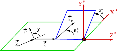
Figure 3: Definition of the scattering and reaction planes. The $X^{*}Y^{*}Z^{*}$ coordinate axes move along with the CM system of the final pion-nucleon and their orientation has been chosen in such a way that the lepton momenta lie in the $O^{*}X^{*}Z^{*}$ plane with the positive $Z^{*}$ axis chosen along $\vec{q}$ and the positive $Y^{*}$ axis chosen along $\vec{k}\wedge\vec{k}^{\,\prime}$.

The cross section in the laboratory (LAB) system is given by

$$\sigma_{{\rm CC}+}=\frac{G_{F}^{2}}{4\pi^{2}|\vec{k}|}\int\frac{d^{3}k^{\prime}}{E^{\prime}}\frac{d^{3}k_{\pi}}{E_{\pi}}\,L^{\mu\nu}(k,k^{\prime})\,W_{\mu\nu}(q,p,k_{\pi}),$$ (11)

where $k^{\mu}=(|\vec{k}\,|,0,0,|\vec{k}\,|)$, $k^{\prime\,\mu}=(E^{\prime},\vec{k}\,^{\prime})$, $p^{\mu}=(M,0,0,0)$, with $M$ the nucleon mass, and $k_{\pi}^{\mu}=(E_{\pi},\vec{k}_{\pi})$ are respectively the four-momenta of the initial lepton, final lepton, initial nucleon and final pion in the LAB frame. Besides, $q=k-k^{\prime}$ is the four-momentum transfer and $G_{F}=1.1664\times 10^{-11}$ MeV^-2 is the Fermi constant. The leptonic tensor is given by

$$L^{\mu\nu}(k,k^{\prime})=k^{\mu}k^{\prime\,\nu}+k^{\nu}k^{\prime\,\mu}-g^{\mu\nu}k\cdot k^{\prime}+i\epsilon^{\mu\nu\alpha\beta}k^{\prime}_{\alpha}k_{\beta},$$ (12)

where we use $\epsilon_{0123}=+1$ and the metric $g^{\mu\nu}={\rm diag}\,(+1,-1,-1,-1)$. The expression is valid both for CC and NC processes induced by neutrinos. For the case of antineutrinos the antisymmetric part of the leptonic tensor changes sign. The hadronic tensor is given by

$$W^{\mu\nu}(q,p,k_{\pi})=\frac{1}{4M}\int\frac{d^{3}p^{\prime}}{(2\pi)^{3}\,2E^{\prime}_{N}}\,\delta^{4}(q+p-p^{\prime}-k_{\pi}){\cal H}^{\mu\nu}(p,p^{\prime},k_{\pi})$$ (13)

with

$${\cal H}^{\mu\nu}(p,p^{\prime},k_{\pi})=\frac{1}{2}\sum_{s,s^{\prime}}\langle N^{\prime}(p^{\prime},s^{\prime})\,\pi(k_{\pi})|J^{\mu}_{{\rm CC}+}(0)|N(p,s)\rangle\langle N^{\prime}(p^{\prime},s^{\prime})\,\pi(k_{\pi})|J^{\nu}_{{\rm CC}+}(0)|N(p,s)\rangle^{*},$$ (14)

being $s$ the helicity of the initial nucleon, and $p^{\prime}=(E^{\prime}_{N},\vec{p}\,^{\prime})$ and $s^{\prime}$, the four-momentum and helicity of the final nucleon, respectively. $J^{\mu}_{{\rm CC}+}(0)$ represents the hadronic current operator for a CC process induced by neutrinos. For CC reactions induced by antineutrinos, we need $J^{\mu}_{{\rm CC}-}(0)=J^{\mu\dagger}_{{\rm CC}+}(0)$, while in the NC case one has to use the corresponding $J^{\mu}_{\rm NC}(0)$ NC operator. In every case, one trivially finds that ${\cal H}^{\mu\nu}$ can be written as the sum of a real symmetric and a pure imaginary antisymmetric parts

$${\cal H}^{\mu\nu}={\cal H}^{\mu\nu}_{s}+i{\cal H}^{\mu\nu}_{a},\quad{\cal H}^{\mu\nu}_{s}=\frac{1}{2}\Big{(}{\cal H}^{\mu\nu}+{\cal H}^{\nu\mu}\Big{)}\in\mathbb{R},\qquad{\cal H}^{\mu\nu}_{a}=-\frac{i}{2}\Big{(}{\cal H}^{\mu\nu}-{\cal H}^{\nu\mu}\Big{)}\in\mathbb{R}.$$ (15)

Making use of the invariant nature of the $L^{\mu\nu}W_{\mu\nu}$ tensor product under a proper Lorentz transformation $\Lambda$, we can write

$$L^{\mu\nu}(k,k^{\prime})W_{\mu\nu}(q,p,k_{\pi})=L^{\mu\nu}(\Lambda k,\Lambda k^{\prime})W_{\mu\nu}(\Lambda q,\Lambda p,\Lambda k_{\pi}),$$ (16)

For each value of $k^{\prime}$, the $\Lambda$ Lorentz transformation is chosen such that the transformed momenta correspond to those measured in the CM of the final pion-nucleon system. The corresponding axes, that we denote as $X^{*}Y^{*}Z^{*}$, are such that $Z^{*+}$ is oriented along $\vec{q}$, $Y^{*+}$ is oriented along $\vec{k}\wedge\vec{k}^{\,\prime}$ and $X^{*+}$ is oriented along $(\vec{k}\wedge\vec{k}^{\,\prime})\wedge\vec{q}$ (see Fig. 3). With the above result, and making the change of variables $\stackrel{{\scriptstyle\to}}{{\Lambda k_{\pi}}}\to\vec{k}^{*}_{\pi}$, for which $d^{3}k_{\pi}/E_{\pi}\to d^{3}k^{*}_{\pi}/E^{*}_{\pi}$, we can rewrite the cross section as

$$\sigma_{{\rm CC}+}=\frac{G_{F}^{2}}{4\pi^{2}|\vec{k}|}\int\frac{d^{3}k^{\prime}}{E^{\prime}}\frac{d^{3}k^{*}_{\pi}}{E^{*}_{\pi}}\,L^{\mu\nu}(\Lambda k,\Lambda k)\,W_{\mu\nu}(\Lambda q,\Lambda p,k^{*}_{\pi}).$$ (17)

In Appendix A we give the value for $\Lambda$ and the corresponding transformed four-momenta that we shall simply denote as $k^{*},k^{\prime*},q^{*},p^{*}$ in what follows. One of the features of the new momenta is that $k^{*},k^{\prime*},q^{*},p^{*}$ do not depend on $\phi^{\prime}$ so that the integral on that variable would just give rise to a factor of $2\pi$. Another salient feature is that the second spatial components of $k^{*}$ and $k^{\prime*}$ are zero. This latter property allows us to immediately identify symmetric and antisymmetric non-diagonal components of the lepton tensor

$$L^{02}(k^{*},k^{\prime*})=-L^{20}(k^{*},k^{\prime*})\ ,\ L^{12}(k^{*},k^{\prime*})=-L^{21}(k^{*},k^{\prime*})\ ,\ L^{23}(k^{*},k^{\prime*})=-L^{32}(k^{*},k^{\prime*}),$$

$$L^{01}(k^{*},k^{\prime*})=L^{10}(k^{*},k^{\prime*})\ ,\ L^{03}(k^{*},k^{\prime*})=L^{30}(k^{*},k^{\prime*})\ ,\ L^{13}(k^{*},k^{\prime*})=L^{31}(k^{*},k^{\prime*}).$$ (18)

In the case of $q^{*}$ and $p^{*}$, both the first and the second spatial components are zero, a fact that will be used below. For $k_{\pi}^{*}$, which is nothing but the four-momentum of the final pion measured in the CM of the final pion-nucleon system, we shall use

$$k_{\pi}^{*\mu}=(E^{*}_{\pi},|\vec{k}^{*}_{\pi}|\sin\theta^{*}_{\pi}\cos\phi^{*}_{\pi},|\vec{k}^{*}_{\pi}|\sin\theta^{*}_{\pi}\sin\phi^{*}_{\pi},|\vec{k}^{*}_{\pi}|\cos\theta^{*}_{\pi}),$$ (19)

where the pion angles are defined with respect to the $X^{*}Y^{*}Z^{*}$ axes (see Fig. 3).

From Eq. (17), we can now write the differential cross section

$$\frac{d\sigma_{{\rm CC}+}}{d\Omega^{\prime}dE^{\prime}d\Omega^{*}_{\pi}}=\frac{|\vec{k}\,^{\prime}|}{|\vec{k}|}\frac{G_{F}^{2}}{4\pi^{2}}\int\frac{|\vec{k}^{*}_{\pi}|^{2}d|\vec{k}^{*}_{\pi}|}{E^{*}_{\pi}}\,L^{\mu\nu}(k^{*},k^{\prime*})\,W_{\mu\nu}(q^{*},p^{*},k^{*}_{\pi}).$$ (20)

The integral in $|\vec{k}^{*}_{\pi}|$ can be easily done using that

$$W_{\mu\nu}(q^{*},p^{*},k^{*}_{\pi})=\frac{1}{4M}\int\frac{d^{3}p^{\prime*}}{2E^{\prime\,*}_{N}}\frac{1}{(2\pi)^{3}}\,\delta^{4}(q^{*}+p^{*}-p^{\prime*}-k^{*}_{\pi})\,{\cal H}_{\mu\nu}(p^{*},p^{\prime*}=p^{*}+q^{*}-k^{*}_{\pi},k^{*}_{\pi}).$$ (21)

After the trivial $d^{3}p^{\prime*}$ integration, there remains a delta of energy conservation that can be used to integrate in $|\vec{k}^{*}_{\pi}|$. One gets

$$\int\frac{|\vec{k}^{*}_{\pi}|^{2}d|\vec{k}^{*}_{\pi}|}{E^{*}_{\pi}}\frac{1}{E^{\prime\,*}_{N}}\delta(W_{\pi N}-E^{\prime\,*}_{N}-E^{*}_{\pi})=\frac{|\vec{k}^{*}_{\pi}|_{0}}{W_{\pi N}},$$ (22)

with $|\vec{k}^{*}_{\pi}|_{0}=\lambda^{1/2}(W_{\pi N}^{2},M^{2},m_{\pi}^{2})/(2W_{\pi N})$ and $\lambda(a,b,c)=(a+b-c)^{2}-4ab$. The differential cross sections can thus be simplified to

$$\frac{d\sigma_{{\rm CC}+}}{d\Omega^{\prime}dE^{\prime}d\Omega^{*}_{\pi}} = \frac{G_{F}^{2}|\vec{k}^{*}_{\pi}|_{0}}{256\pi^{5}MW_{\pi N}}\frac{|\vec{k}^{\prime}|}{|\vec{k}|}\,L^{\mu\nu}(k^{*},k^{\prime*})\,{\cal H}_{\mu\nu}(p^{*},p^{\prime*}=p^{*}+q^{*}-k^{*}_{\pi},k^{*}_{\pi}),$$ (23)

Changing variables from $(\theta^{\prime},E^{\prime})\to\left(Q^{2}=-q^{2},W_{\pi N}=\sqrt{(q+p)^{2}}\,\right)$, we further obtain

$$\frac{d\sigma_{{\rm CC}+}}{dQ^{2}dW_{\pi N}d\Omega^{*}_{\pi}} = \frac{G_{F}^{2}|\vec{k}^{*}_{\pi}|_{0}}{256\pi^{4}M^{2}|\vec{k}|^{2}}\,\,L^{\mu\nu}(k^{*},k^{\prime*})\,{\cal H}_{\mu\nu}(p^{*},p^{\prime*}=p^{*}+q^{*}-k^{*}_{\pi},k^{*}_{\pi}),$$ (24)

where the trivial dependence on $\phi^{\prime}$ (final lepton laboratory azimuthal angle) has been integrated out giving rise to a factor of $2\pi$.

III.1 The $\phi^{*}_{\pi}$ dependence of the ${d\sigma_{{\rm CC}+}}/({d\Omega^{\prime}dE^{\prime}d\Omega^{*}_{\pi}})$ and ${d\sigma_{{\rm CC}+}}/({dQ^{2}dW_{\pi N}d\Omega^{*}_{\pi}})$ differential cross sections

The $\phi^{*}_{\pi}$ dependence of the differential cross section can be isolated using very general arguments. For that purpose, let us consider the active rotation $\hat{R}$ defined as

$$\hat{R}^{\mu}_{\ \nu}=\left(\begin{array}[]{cccc}1&0&0&0\\ 0&\cos\phi^{*}_{\pi}&-\sin\phi^{*}_{\pi}&0\\ 0&\sin\phi^{*}_{\pi}&\cos\phi^{*}_{\pi}&0\\ 0&0&0&1\end{array}\right),$$ (29)

which is such that

$$(\hat{R}^{-1}k^{*}_{\pi})^{\mu}=(E^{*}_{\pi},|\vec{k}^{*}_{\pi}|\sin\theta^{*}_{\pi},0,|\vec{k}^{*}_{\pi}|\cos\theta^{*}_{\pi}),$$ (30)

while $\hat{R}^{-1}q^{*}=q^{*},\ \hat{R}^{-1}p^{*}=p^{*}$. Thus, making use of the tensor character of $W^{\mu\nu}(q^{*},p^{*},k^{*}_{\pi})$, we will have

$$W^{\mu\nu}=W^{\mu\nu}(q^{*},p^{*},k^{*}_{\pi}) = W^{\mu\nu}(\hat{R}\hat{R}^{-1}q^{*},\hat{R}\hat{R}^{-1}p^{*},\hat{R}\hat{R}^{-1}k^{*}_{\pi})$$ (31)

$$= \hat{R}^{\mu}_{\ \ \alpha}\hat{R}^{\nu}_{\ \ \beta}\ W^{\alpha\beta}(\hat{R}^{-1}q^{*},\hat{R}^{-1}p^{*},\hat{R}^{-1}k^{*}_{\pi})$$

$$= \hat{R}^{\mu}_{\ \ \alpha}\hat{R}^{\nu}_{\ \ \beta}\ W^{\alpha\beta}(q^{*},p^{*},{\hat{R}^{-1}k^{*}_{\pi}})=\hat{R}^{\mu}_{\ \ \alpha}\hat{R}^{\nu}_{\ \ \beta}\ \widetilde{W}^{\alpha\beta}$$

where, for short, we have introduced the notation

$$W^{\mu\nu}=W^{\mu\nu}(q^{*},p^{*},k^{*}_{\pi})\ \ ,\ \ \widetilde{W}^{\mu\nu}=W^{\mu\nu}(q^{*},p^{*},{\hat{R}^{-1}k^{*}_{\pi}})=W^{\mu\nu}\big{|}_{\phi^{*}_{\pi}=0}.$$ (32)

It is interesting to note that, since the second spatial components of $q^{*},p^{*},\hat{R}^{-1}k^{*}_{\pi}$ are zero, the non-zero contributions to the $\widetilde{W}^{a2}$ and $\widetilde{W}^{2a}$ components of the hadronic tensor for $a=0,1,3$ should always involve terms constructed using the Levi-Civita pseudotensor, $v^{a}\epsilon^{2\alpha\beta\rho}q^{*}_{\alpha}p^{*}_{\beta}(\hat{R}^{-1}k^{*}_{\pi})_{\rho}$ or $\epsilon^{2a\alpha\beta}v_{\alpha}w_{\beta}$ with $v\neq w$ being any of the four-vectors $q^{*},p^{*},\hat{R}^{-1}k^{*}_{\pi}$. On the other hand, any component of the type $\widetilde{W}^{ab}$, with $a,b=0,1,3$, cannot contain the Levi-Civita pseudotensor, because the coordinate 2 will appear in the contraction of the pseudotensor with the available vectors, and none of them has a spatial component in the $Y^{*}$ axis.

In the case of photo- or electropion production on unpolarized nucleons, and since the electromagnetic interaction conserves parity , one has

$$\widetilde{W}^{a2}_{em}=\widetilde{W}^{2a}_{em}=0,\ a=0,1,3.$$ (33)

Going back to the $\phi^{*}_{\pi}$ dependence of $W^{\mu\nu}$, we see that it is now fully contained in $\hat{R}$. Thus, performing the rotations in Eq. (31), the different components of the tensor $W^{\mu\nu}$ can be written in terms of $\widetilde{W}^{\mu\nu}=W^{\mu\nu}\big{|}_{\phi^{*}_{\pi}=0}$ and the pion azimuthal angle $\phi^{*}_{\pi}$. The explicit expressions are given in Eq. (82) of Appendix B, from where it follows that the possible dependencies are $1,\cos\phi^{*}_{\pi},\cos 2\phi^{*}_{\pi},\sin\phi^{*}_{\pi}$ and $\sin 2\phi^{*}_{\pi}$, as discussed in detail also in Refs. Hernández et al. (2007a, b); Sato et al. (2003). We have then

$$\frac{d\sigma_{{\rm CC}+}}{d\Omega^{\prime}dE^{\prime}d\Omega^{*}_{\pi}} = \frac{|\vec{k}^{\prime}|}{|\vec{k}|}\frac{G_{F}^{2}}{4\pi^{2}}\Big{(}A^{*}+B^{*}\cos\phi^{*}_{\pi}+C^{*}\cos 2\phi^{*}_{\pi}+D^{*}\sin\phi^{*}_{\pi}+E^{*}\sin 2\phi^{*}_{\pi}\Big{)},$$

$$\frac{d\sigma_{{\rm CC}+}}{dQ^{2}dW_{\pi N}d\Omega^{*}_{\pi}} = \frac{G_{F}^{2}W_{\pi N}}{4\pi M|\vec{k}|^{2}}\Big{(}A^{*}+B^{*}\cos\phi^{*}_{\pi}+C^{*}\cos 2\phi^{*}_{\pi}+D^{*}\sin\phi^{*}_{\pi}+E^{*}\sin 2\phi^{*}_{\pi}\Big{)},$$ (34)

with the $A^{*},B^{*},C^{*},D^{*}$ and $E^{*}$ structure functions given by

$$A^{*} = \int\frac{|\vec{k}^{*}_{\pi}|^{2}d|\vec{k}^{*}_{\pi}|}{E^{*}_{\pi}}\,\Big{[}L^{00}\,\widetilde{W}_{00}^{(s)}+2L^{03}\,\widetilde{W}_{03}^{(s)}+L^{33}\,\widetilde{W}_{33}^{(s)}+\frac{1}{2}(L^{11}+L^{22})\,\left(\widetilde{W}_{11}^{(s)}+\widetilde{W}_{22}^{(s)}\right)+2iL^{12}\,\widetilde{W}_{12}^{(a)}\Big{]},$$

$$B^{*} = \int\frac{|\vec{k}^{*}_{\pi}|^{2}d|\vec{k}^{*}_{\pi}|}{E^{*}_{\pi}}\,2\Big{[}L^{01}\,\widetilde{W}_{01}^{(s)}+L^{13}\,\widetilde{W}_{13}^{(s)}+iL^{02}\,\widetilde{W}_{02}^{(a)}+iL^{23}\,\widetilde{W}_{23}^{(a)}\Big{]},$$

$$C^{*} = \int\frac{|\vec{k}^{*}_{\pi}|^{2}d|\vec{k}^{*}_{\pi}|}{E^{*}_{\pi}\,}\frac{1}{2}\left[(L^{11}-L^{22})\,\left(\widetilde{W}_{11}^{(s)}-\widetilde{W}_{22}^{(s)}\right)\right],$$

$$D^{*} = \int\frac{|\vec{k}^{*}_{\pi}|^{2}d|\vec{k}^{*}_{\pi}|}{E^{*}_{\pi}}\,2\Big{[}-L^{01}\,\widetilde{W}_{02}^{(s)}-L^{13}\,\widetilde{W}_{23}^{(s)}+iL^{02}\,\widetilde{W}_{01}^{(a)}+iL^{23}\,\widetilde{W}_{13}^{(a)}\Big{]},$$

$$E^{*} = \int\frac{|\vec{k}^{*}_{\pi}|^{2}d|\vec{k}^{*}_{\pi}|}{E^{*}_{\pi}}\,\left[(L^{22}-L^{11})\,\widetilde{W}_{12}^{(s)}\right],$$ (35)

where we have made use of Eq. (18), and we have denoted $L^{\mu\nu}=L^{\mu\nu}(k^{*},k^{\prime*})$ for simplicity. In addition, following Eq. (15), we have split the hadron tensor into symmetric ($\widetilde{W}_{\mu\nu}^{(s)}$) and antisymmetric ($\widetilde{W}_{\mu\nu}^{(a)}$) parts,

$$\widetilde{W}_{\mu\nu}=\widetilde{W}_{\mu\nu}^{(s)}+i\,\widetilde{W}_{\mu\nu}^{(a)},\qquad\widetilde{W}_{\mu\nu}^{(s,a)}\in\mathbb{R}$$ (36)

Thus, and thanks to the fact that $L^{a2}$ ($a=0,1,3$) is purely imaginary while the rest of the components of the lepton tensor are real, we trivially confirm that all $A^{*},B^{*},C^{*},D^{*}$ and $E^{*}$ structure functions are real.

Besides, since

$$W^{\mu\nu}\pm W^{\nu\mu}=\hat{R}^{\mu}_{\ \ \alpha}\hat{R}^{\nu}_{\ \ \beta}\,\left(\widetilde{W}^{\alpha\beta}\pm\widetilde{W}^{\beta\alpha}\right)\,$$ (37)

we have that the symmetric and antisymmetric parts of $W^{\mu\nu}$ are determined respectively from $\widetilde{W}_{\mu\nu}^{(s)}$ and $\widetilde{W}_{\mu\nu}^{(a)}$ using the same rotation. Therefore, we can conclude that the $C^{*}$ and $E^{*}$ structure constants are generated from the contraction of the symmetric parts of the lepton and hadronic tensors, while $A^{*},B^{*}$ and $D^{*}$ also get contributions from the contraction of the antisymmetric parts of the lepton and hadronic tensors (see also Eqs. A8 and A9 of Ref. Hernández et al. (2007a)). As already mentioned, the antisymmetric part of the lepton tensor changes sign for the case of antineutrino induced reactions. Note also that from Eq. (33), it trivially follows that for electropion production off unpolarized nucleons, the $E^{*}$ structure function vanishes, i.e., there is no $\sin 2\phi^{*}_{\pi}$ term in the differential cross section. Moreover, the symmetric contribution to $D^{*}$ will also vanish. Thus, the dependence on $\sin\phi^{*}_{\pi}$ will only survive for polarized electrons, for which the lepton tensor has an antisymmetric part that leads to non-zero $L^{02}$ and $L^{23}$ components (see Eq. (18)).

The above differential cross sections can be written as a sum over differential cross sections, $d\sigma(W^{*}N\to N^{\prime}\pi)/d\Omega^{*}_{\pi}\big{|}_{\phi^{*}_{\pi}=0}$, for virtual $W$ of different polarizations. This relation is given, in the zero lepton mass limit, in Eq. (104) of Appendix C. Such a limit is exact for NC processes and provides an excellent approximation for CC processes induced by electron neutrinos.

III.2 Parity violation in the ${d\sigma_{{\rm CC}+}}/({d\Omega^{\prime}dE^{\prime}d\Omega^{*}_{\pi}})$ and ${d\sigma_{{\rm CC}+}}/({dQ^{2}dW_{\pi N}d\Omega^{*}_{\pi}})$ differential cross sections

The terms proportional to $\sin\phi^{*}_{\pi}$ and $\sin 2\phi^{*}_{\pi}$ in Eq. (34) give rise to parity violation in the weak ${d\sigma}/({d\Omega^{\prime}dE^{\prime}d\Omega^{*}_{\pi}})$ and ${d\sigma}/({dQ^{2}dW_{\pi N}d\Omega^{*}_{\pi}})$ differential cross sections Hernández et al. (2007a, b). The reason is the following. After a parity transformation $\vec{k},\vec{k}\,^{\prime},\vec{q}=\vec{k}-\vec{k}\,^{\prime},\vec{p}$ and $\vec{k}_{\pi}$ change direction ($\vec{v}\to\vec{v}_{P}=-\vec{v}\,$). The new $Z^{*+}_{P}\equiv\vec{q}_{P}$ and $X^{*+}_{P}\equiv(\vec{k}_{P}\wedge\vec{k}^{\prime}_{P})\wedge\vec{q}_{P}$ axes also change direction accordingly, but $Y^{*+}_{P}\equiv\vec{k}_{P}\wedge\vec{k}^{\prime}_{P}$ does not. Measured in the new $X^{*}_{P}Y^{*}_{P}Z^{*}_{P}$ system we have that the transformed four-vectors $k^{*},k^{\prime*},q^{*}$ and $p^{*}$ have exactly the same components as before the parity transformation, since none of these vectors has components along the $Y^{*}$ axis. However, the pion momentum does have a component along the $Y^{*}$ axis and therefore the values of $\theta^{*}_{\pi}$ and $\phi^{*}_{\pi}$ for the reversed pion momentum measured with respect to the new $X^{*}_{P}Y^{*}_{P}Z^{*}_{P}$ system change now as

$$\theta^{*}_{\pi}\to\theta^{*}_{\pi}\ \ ,\ \ \phi^{*}_{\pi}\to 2\pi-\phi^{*}_{\pi}.$$

As a result, $L^{\mu\nu}$ and $\widetilde{W}_{\mu\nu}=W^{\mu\nu}\big{|}_{\phi^{*}_{\pi}=0}$ remain the same and thus the $A^{*},B^{*},C^{*},D^{*}$ and $E^{*}$ structure functions do not change. However, for the $\phi^{*}_{\pi}$ dependence we have that

$$\cos\phi^{*}_{\pi}\to\cos(2\pi-\phi^{*}_{\pi})=\cos\phi^{*}_{\pi},$$

$$\cos 2\phi^{*}_{\pi}\to\cos\big{(}2(2\pi-\phi^{*}_{\pi})\big{)}=\cos 2\phi^{*}_{\pi},$$

$$\sin\phi^{*}_{\pi}\to\sin(2\pi-\phi^{*}_{\pi})=-\sin\phi^{*}_{\pi},$$

$$\sin 2\phi^{*}_{\pi}\to\sin\big{(}2(2\pi-\phi^{*}_{\pi})\big{)}=-\sin 2\phi^{*}_{\pi}.$$ (38)

The sign change in the $\sin\phi^{*}_{\pi}$ and $\sin 2\phi^{*}_{\pi}$ terms implies that the $D^{*}$ and $E^{*}$ contributions to the differential cross sections violate parity. Parity violation in weak production is then reflected by the fact that the pion angular distributions above and below the scattering plane are different (see the discussion of Fig. 18 in Sec. IV.2). Note, however, that after integrating in $\phi^{*}_{\pi}$, the parity breaking terms cancel, and one obtains that the ${d\sigma_{{\rm CC}+}}/({d\Omega^{\prime}dE^{\prime}d\cos\theta^{*}_{\pi}})$ and ${d\sigma_{{\rm CC}+}}/({dQ^{2}dW_{\pi N}d\cos\theta^{*}_{\pi}})$ differential cross sections are invariant under parity.

From the discussion below Eq. (32), one notices that the structure functions $A^{*},B^{*}$ and $C^{*}$ always involve either symmetric hadron tensor terms that do not contain the Levi-Civita pseudotensor, or antisymmetric hadron tensor terms constructed using the Levi-Civita pseudotensor. In turn, $D^{*}$ and $E^{*}$ always involve either symmetric hadron tensor terms constructed using the Levi-Civita pseudotensor, or antisymmetric hadron tensor terms that do not contain the Levi-Civita pseudotensor. Using the terminology of Refs. Hernández et al. (2007a, b), the structure functions $A^{*},B^{*}$ and $C^{*}$ ($D^{*}$ and $E^{*}$) are therefore constructed out of the parity conserving (violating) hadron tensors (see for instance Eq. A1 of Ref. Hernández et al. (2007a) and the related discussion).

A further remark concerns time-reversal (T). As discussed in Refs. Hernández et al. (2007a, b), the $\sin\phi^{*}_{\pi}$ and $\sin 2\phi^{*}_{\pi}$ terms encode T-odd correlations. However, the existence of these terms does not necessarily mean that there exists a violation of T-invariance in the process because of the existence of strong final state interaction effects Karpman et al. (1968); Cannata et al. (1970).

There is a subtlety, worth mentioning, for the case of pion production induced by initial polarized electrons. Following the above discussion, one could wrongly conclude that there exists parity violation in these processes. This is because, as commented before, though the $\sin 2\phi^{*}_{\pi}$ contribution is absent, the $L^{02}_{em}$ and $L^{23}_{em}$ terms in $D^{*}\sin\phi^{*}_{\pi}$ survive, since they do not involve the vanishing $\widetilde{W}^{a2}_{em}$ and $\widetilde{W}^{2a}_{em}$ components. What happens is that $L^{02}_{em}$ and $L^{23}_{em}$ change sign under a parity transformation, contrary to the weak pion production case. This is because the antisymmetric part of the electromagnetic lepton tensor is proportional to the helicity, $h$, of the initial electron ($\propto h\epsilon^{\mu\nu\rho\sigma}k^{*}_{\rho}k^{\prime*}_{\sigma}$). The helicity is a pseudoscalar and it changes sign under parity, which induces also a change of sign in $L^{02}_{em}$ and $L^{23}_{em}$ that compensates the change of sign under parity of $\sin\phi^{*}_{\pi}$. As a consequence $D^{*}\sin\phi^{*}_{\pi}$ remains parity invariant. With respect to time reversal, the helicity does not change sign under T, and thus the lepton tensors in electro– and weak–pion production behave in the same way under time reversal transformations, and therefore T–odd correlations exist also in the case of electromagnetic reactions.

III.2.1 Origin of the parity conserving and parity violating contributions to the hadronic tensor

In this section, we will use the terminology parity conserving (PC) and parity violating (PV) terms to refer to contributions to the hadronic tensor that give rise to parity conservation/violation when contracted with the leptonic tensor. Taking into account the structure of the leptonic tensor, where the symmetric part is a true tensor while the antisymmetric part is proportional to the Levi-Civita pseudotensor, it is clear that (i) any symmetric part in the hadron tensor that contains a Levi-Civita pseudotensor or (ii) any antisymmetric part in the hadron tensor that does not contain a Levi-Civita pseudotensor are PV ones Hernández et al. (2007a, b). We have explicitly seen this in the expressions of $D^{*}$ and $E^{*}$ of Eq. (35), as we pointed out above in the main body of Subsec. III.2 (we recall here again the discussion of Eq. (37), where we have shown that the symmetric and antisymmetric parts of the tensors $W^{\mu\nu}$ and $\widetilde{W}^{\mu\nu}$ are connected by the rotations of Eq. (31)). As we are going to show in the following, the PV terms originate from the interference between different contributions to the hadronic current that are not relatively real.

For our purposes, it is enough to consider the nucleon tensor defined in Eq. (14) associated to $\widetilde{W}^{\mu\nu}$ (independent of $\phi^{*}_{\pi}$), that can be written as the trace

$${\cal\widetilde{H}}^{\mu\nu}(p^{*},p^{\prime*},\hat{R}^{-1}k^{*}_{\pi})= \frac{1}{2}{\rm Tr}\left[(/p^{\prime*}+M){\cal J}^{\mu}(p^{*},p^{\prime*},\hat{R}^{-1}k^{*}_{\pi})(/p+M)\gamma^{0}{\cal J}^{\nu\,\dagger}(p^{*},p^{\prime*},\hat{R}^{-1}k^{*}_{\pi})\gamma^{0}\right],$$ (39)

where here $p^{\prime*}=q^{*}+p^{*}-\hat{R}^{-1}k^{*}_{\pi}$, and ${\cal J}^{\mu}(p^{*},p^{\prime*},\hat{R}^{-1}k^{*}_{\pi})$ is defined from the hadronic current operator matrix element

$$\langle N^{\prime}(p^{\prime*},s^{\prime})\,\pi(\,\hat{R}^{-1}k^{*}_{\pi})|J^{\mu}_{{\rm CC}+}(0)|N(p^{*},s)\rangle=\bar{u}_{s^{\prime}}(p^{\prime*}){\cal J}^{\mu}(p^{*},p^{\prime*},\hat{R}^{-1}k^{*}_{\pi})\,u_{s}(p^{*}).$$ (40)

The amputated ${\cal J}^{\mu}(p^{*},p^{\prime*},\hat{R}^{-1}k^{*}_{\pi})$ current contains a vector and an axial contribution that one can write as

$${\cal J}^{\mu}(p^{*},p^{\prime*}\,\hat{R}^{-1}k^{*}_{\pi})=\sum_{j_{1}}\gamma_{5}e^{i\varphi_{Vj_{1}}(p^{*},p^{\prime*}\,\hat{R}^{-1}k^{*}_{\pi})}{\cal J}^{\mu}_{Vj_{1}}(p^{*},p^{\prime*},\hat{R}^{-1}k^{*}_{\pi})+\sum_{j_{2}}e^{i\varphi_{Aj_{2}}(p^{*},p^{\prime*},\hat{R}^{-1}k^{*}_{\pi})}{\cal J}^{\mu}_{Aj_{2}}(p^{*},p^{\prime*},\hat{R}^{-1}k^{*}_{\pi}).$$

(41)

where the ${\cal J}^{\mu}_{Vj}$ and ${\cal J}^{\mu}_{Aj}$ correspond to the different Dirac operator structures present in the hadronic current. They are built from $\gamma$ matrices (no $\gamma_{5}$ however) and momenta and, for each term in the two sums, $e^{i\varphi_{Vj}(p^{*},p^{\prime*},\hat{R}^{-1}k^{*}_{\pi})}$ and $e^{i\varphi_{Aj}(p^{*},p^{\prime*},\hat{R}^{-1}k^{*}_{\pi})}$ stand for the global phase of all multiplicative factors in that term other than $\gamma$ matrices. Note that for the HNV model there is a correspondence between the phases $\varphi_{A}$ and $\varphi_{V}$ and the complex structure of the $\Delta$ (corrected by the Olsson phases introduced in Eq. (6) and the $D_{13}$(1520) resonance). However, for the DCC and SL models, in addition to the complex structure of the resonances ($m_{R}$ and $\Gamma_{R}$) one should account for loop effects that provide further relative phases between different contributions to the amplitude. Simplifying the notation, we will have

$${\cal\widetilde{H}}^{\mu\nu} = \frac{1}{2}{\rm Tr}\Bigg{[}(/p^{\prime*}+M)\Big{[}\sum_{j_{1}}\gamma_{5}e^{i\varphi_{Vj_{1}}}{\cal J}^{\mu}_{Vj_{1}}+\sum_{j_{2}}e^{i\varphi_{Aj_{2}}}{\cal J}^{\mu}_{Aj_{2}}\Big{]}(/p^{*}+M)\gamma^{0}\Big{[}\sum_{k_{1}}e^{-i\varphi_{Vk_{1}}}{\cal J}^{\nu\,\dagger}_{Vk_{1}}\gamma_{5}+\sum_{k_{2}}e^{-i\varphi_{Ak_{2}}}{\cal J}^{\nu\,\dagger}_{Ak_{2}}\Big{]}\gamma^{0}\Bigg{]}$$ (42)

that can be split into two contributions ${\cal\widetilde{H}}^{\mu\nu}={\cal\widetilde{H}}^{\mu\nu}_{VV+AA}+{\cal\widetilde{H}}^{\mu\nu}_{VA+AV}$, given by

$${\cal\widetilde{H}}^{\mu\nu}_{VV+AA} = \hskip 9.95863pt\frac{1}{2}\sum_{j_{1}}\sum_{k_{1}}e^{i(\varphi_{Vj_{1}}-\varphi_{Vk_{1}})}\,{\rm Tr}\left[(/p^{\prime*}-M){\cal J}^{\mu}_{Vj_{1}}(/p^{*}+M)\gamma^{0}{\cal J}^{\nu\,\dagger}_{Vk_{1}}\gamma^{0}\right]$$

$$+\frac{1}{2}\sum_{j_{2}}\sum_{k_{2}}e^{i(\varphi_{Aj_{2}}-\varphi_{Ak_{2}})}\,{\rm Tr}\left[(/p^{\prime*}+M){\cal J}^{\mu}_{Aj_{2}}(/p^{*}+M)\gamma^{0}{\cal J}^{\nu\,\dagger}_{Ak_{2}}\gamma^{0}\right]$$

$${\cal\widetilde{H}}^{\mu\nu}_{VA+AV} = -\frac{1}{2}\sum_{j_{1}}\sum_{j_{2}}e^{i(\varphi_{Vj_{1}}-\varphi_{Aj_{2}})}\,{\rm Tr}\left[(/p^{\prime*}-M){\cal J}^{\mu}_{Vj_{1}}(/p^{*}+M)\gamma^{0}{\cal J}^{\nu\,\dagger}_{Aj_{2}}\gamma^{0}\gamma_{5}\right]$$ (43)

$$-\frac{1}{2}\sum_{j_{1}}\sum_{j_{2}}e^{-i(\varphi_{Vj_{1}}-\varphi_{Aj_{2}})}\,{\rm Tr}\left[(/p^{\prime*}+M){\cal J}^{\mu}_{Aj_{2}}(/p^{*}+M)\gamma^{0}{\cal J}^{\nu\,\dagger}_{Vj_{1}}\gamma^{0}\gamma_{5}\right].$$

Let us pay attention first to ${\cal\widetilde{H}}^{\mu\nu}_{VV+AA}$. Since the two traces are real, we therefore get real symmetric contributions to the hadronic tensor, ${\cal\widetilde{H}}^{\mu\nu\,(s)}_{VV+AA}$, given by

$$\underbrace{{\cal\widetilde{H}}^{\mu\nu\,(s)}_{VV+AA}}_{\rm PC} = \hskip 9.95863pt\frac{1}{2}\sum_{j_{1}}\sum_{k_{1}}\cos(\varphi_{Vj_{1}}-\varphi_{Vk_{1}}){\rm Tr}\left[(/p^{\prime*}-M){\cal J}^{\mu}_{Vj_{1}}(/p^{*}+M)\gamma^{0}{\cal J}^{\nu\,\dagger}_{Vk_{1}}\gamma^{0}\right]$$ (45)

$$+\frac{1}{2}\sum_{j_{2}}\sum_{k_{2}}\cos(\varphi_{Aj_{2}}-\varphi_{Ak_{2}}){\rm Tr}\left[(/p^{\prime*}+M){\cal J}^{\mu}_{Aj_{2}}(/p^{*}+M)\gamma^{0}{\cal J}^{\nu\,\dagger}_{Ak_{2}}\gamma^{0}\right],$$

and purely imaginary antisymmetric contributions, $i{\cal\widetilde{H}}^{\mu\nu\,(a)}_{VV+AA}$, given by (in this case we have a sine which is an odd function)

$$\underbrace{i{\cal\widetilde{H}}^{\mu\nu\,(a)}_{VV+AA}}_{\rm PV} = \hskip 9.95863pt\frac{i}{2}\sum_{j_{1}\neq k_{1}}\sin(\varphi_{Vj_{1}}-\varphi_{Vk_{1}}){\rm Tr}\left[(/p^{\prime*}-M){\cal J}^{\mu}_{Vj_{1}}(/p^{*}+M)\gamma^{0}{\cal J}^{\nu\,\dagger}_{Vk_{1}}\gamma^{0}\right]$$ (46)

$$+\frac{i}{2}\sum_{j_{2}\neq k_{2}}\sin(\varphi_{Aj_{2}}-\varphi_{Ak_{2}}){\rm Tr}\left[(/p^{\prime*}+M){\cal J}^{\mu}_{Aj_{2}}(/p^{*}+M)\gamma^{0}{\cal J}^{\nu\,\dagger}_{Ak_{2}}\gamma^{0}\right].$$

The symmetric part, ${\cal\widetilde{H}}^{\mu\nu\,(s)}_{VV+AA}$, does not contain a Levi-Civita pseudotensor and it is thus PC since when it is contracted with the symmetric part of the leptonic tensor it will give rise to a true scalar. On the other hand, the antisymmetric part, ${\cal\widetilde{H}}^{\mu\nu\,(a)}_{VV+AA}$, does not contain a Levi-Civita pseudotensor either; it is thus PV since when it is contracted with the antisymmetric part of the leptonic tensor it will give rise to a pseudoscalar.

With respect to ${\cal\widetilde{H}}^{\mu\nu}_{VA+AV}$, we see that in this case the traces involved are purely imaginary and contain a Levi-Civita pseudotensor. Then, it gives rise to purely imaginary and antisymmetric contributions, ${\cal\widetilde{H}}^{\mu\nu\,(a)}_{VA+AV}$, to the hadronic tensor given by

$$\underbrace{i{\cal\widetilde{H}}^{\mu\nu\,(a)}_{VA+AV}}_{\rm PC} = -\frac{1}{2}\sum_{j_{1}}\sum_{j_{2}}\cos(\varphi_{Vj_{1}}-\varphi_{Aj_{2}})\Bigg{\{}{\rm Tr}\left[(/p^{\prime*}-M){\cal J}^{\mu}_{Vj_{1}}(/p^{*}+M)\gamma^{0}{\cal J}^{\nu\,\dagger}_{Aj_{2}}\gamma^{0}\gamma_{5}\right]$$ (48)

$$+{\rm Tr}\left[(/p^{\prime*}+M){\cal J}^{\mu}_{Aj_{2}}(/p^{*}+M)\gamma^{0}{\cal J}^{\nu\,\dagger}_{Vj_{1}}\gamma^{0}\gamma_{5}\right]\Bigg{\}}.$$

and to real symmetric contributions, ${\cal\widetilde{H}}^{\mu\nu\,(s)}_{VA+AV}$ given by

$$\underbrace{{\cal\widetilde{H}}^{\mu\nu\,(s)}_{VA+AV}}_{\rm PV} = -\frac{i}{2}\sum_{j_{1}}\sum_{j_{2}}\sin(\varphi_{Vj_{1}}-\varphi_{Aj_{2}})\Bigg{\{}{\rm Tr}\left[(/p^{\prime*}-M){\cal J}^{\mu}_{Vj_{1}}(/p^{*}+M)\gamma^{0}{\cal J}^{\nu\,\dagger}_{Aj_{2}}\gamma^{0}\gamma_{5}\right]$$ (49)

$$-{\rm Tr}\left[(/p^{\prime*}+M){\cal J}^{\mu}_{Aj_{2}}(/p^{*}+M)\gamma^{0}{\cal J}^{\nu\,\dagger}_{Vj_{1}}\gamma^{0}\gamma_{5}\right]\Bigg{\}},$$

The symmetric part, ${\cal\widetilde{H}}^{\mu\nu\,(s)}_{VA+AV}$, is now PV since it contains a Levi-Civita pseudotensor coming from the trace, whereas the antisymmetric part, ${\cal\widetilde{H}}^{\mu\nu\,(a)}_{VA+AV}$, is PC for the same reason. Note that Eqs (45), (46), (48) and (49) show explicitly the decomposition

$${\cal\widetilde{H}}_{\mu\nu}={\cal\widetilde{H}}_{\mu\nu}^{(s)}+i\,{\cal\widetilde{H}}_{\mu\nu}^{(a)},\qquad{\cal\widetilde{H}}_{\mu\nu}^{(s,a)}\in\mathbb{R}$$ (50)

which trivially leads to that of the tensor ${\widetilde{W}}_{\mu\nu}$ in Eq. (36).

As we have just shown, the PV terms are always proportional to the sine of phase differences and they would cancel exactly if all contributions to the hadronic current were relatively real. These PV terms give rise to the $\sin\phi^{*}_{\pi}$ and $\sin 2\phi^{*}_{\pi}$ terms in the differential cross sections in Eq. (34). As seen in Eq. (35), $E^{*}$ is given in terms of a symmetric contribution to the hadronic tensor ($\widetilde{W}^{(s)}_{12}$) that involves Levi-Civita tensors, and thus the $\sin 2\phi^{*}_{\pi}$ dependence in the differential cross section must come necessarily from the symmetric ${\cal\widetilde{H}}^{\mu\nu\,(s)}_{VA+AV}$ PV term. The latter is generated from vector-axial interference and then it will be absent in the case of photo- or electro-production. On the other hand, the $\sin\phi^{*}_{\pi}$ dependence in the differential cross section gets contributions from both PV terms: the symmetric ${\cal\widetilde{H}}^{\mu\nu\,(s)}_{VA+AV}$ and the antisymmetric ${\cal\widetilde{H}}^{\mu\nu\,(a)}_{VV+AA}$ tensors, which give rise to $\widetilde{W}^{(s)}_{02,23}$ and $\widetilde{W}^{(a)}_{01,13}$, respectively. The former (symmetric) ones contain Levi-Civita tensors, while the latter (antisymmetric) ones do not. We remark that ${\cal\widetilde{H}}^{\mu\nu\,(a)}_{VV+AA}$ is generated from vector-vector and axial-axial interferences, and the $VV$ part will also appear in polarized electron scattering. The PV hadron tensors also lead to time-reversal odd correlations in the amplitudes (see discussion in Refs. Hernández et al. (2007b, a)).

In the case of the HNV model, neglecting for simplicity in the discussion the $D_{13}(1520)$ contribution, and in the absence of Olsson phases, those PV terms can only be generated by the interference between the part of the $\Delta P$ contribution that is proportional to the $\Delta$ propagator and all other non-resonant terms Hernández et al. (2007a). They are not relatively real due to the presence of a nonzero $\Delta$ width in the $\Delta$ propagator. Once the Olsson phases are included, there are other sources of parity violation in the model like the interference between the contact term generated from the $\Delta P$ amplitude by the $c\,\delta P_{\mu\nu}(p_{\Delta})$ term in Eq. (7) and the background, or the interference between the vector and axial parts of the contact term in $\Delta P$.

In the case of the SL and DCC models, the unitarization procedure guarantees that, for energies below the two pion production threshold, each amplitude ${\cal M}$ corresponding to a given isospin, total angular momentum and pion orbital angular momentum, is given by $e^{i\delta}|{\cal M}|$, with $\delta$ the corresponding $\pi N$ phase shift for the given quantum numbers. In this case it is better to work in a multipole language. For that, we can rewrite

$${\cal\widetilde{H}}^{\mu\nu}(p^{*},p^{\prime*},\hat{R}^{-1}k^{*}_{\pi})= \frac{1}{2}{\rm Tr}\left[h^{\mu}(p^{*},p^{\prime*},\hat{R}^{-1}k^{*}_{\pi})h^{\nu\,\dagger}(p^{*},p^{\prime*},\hat{R}^{-1}k^{*}_{\pi})\right],$$ (51)

with $h^{\mu}(p^{*},p^{\prime*},\hat{R}^{-1}k^{*}_{\pi})$ and the ${\cal J}^{\mu}(p^{*},p^{\prime*},\hat{R}^{-1}k^{*}_{\pi})$ of Eq. (40) related via

$$\bar{u}_{s^{\prime}}(p^{\prime*}){\cal J}^{\mu}(p^{*},p^{\prime*},\hat{R}^{-1}k^{*}_{\pi})\,u_{s}(p^{*})=\chi^{\dagger}_{s^{\prime}}h^{\mu}(p^{*},p^{\prime*},\hat{R}^{-1}k^{*}_{\pi})\chi_{s},$$ (52)

with $\chi_{s,s^{\prime}}$ Pauli bispinors. Since the main objective is to see the origin of the PV terms, we use in what follows a very simplified notation. Corresponding full expressions can be found for instance in Refs. Sato and Lee (2009); Adler (1968). One can expand

$$h^{\mu}=\sum_{j_{1}}e^{i\delta_{j_{1}}}(|M_{Vj_{1}}|{\cal O}_{Vj_{1}}^{\mu}-|M_{Aj_{1}}|{\cal O}_{Aj_{1}}^{\mu})$$ (53)

where the sum is over all possible multipoles and the ${\cal O}_{V,A}^{\mu}$ operators are constructed from Pauli matrices and momenta. The ${\cal O}_{V}^{\mu}$ operators violate parity while the ${\cal O}_{A}^{\mu}$ ones do not. Then,

$${\cal\widetilde{H}}^{\mu\nu}=\frac{1}{2}\sum_{j_{1}}\sum_{j_{2}}e^{i(\delta_{j_{1}}-\delta_{j_{2}})}{\rm Tr}\left[(|M_{Vj_{1}}|{\cal O}_{Vj_{1}}^{\mu}-|M_{Aj_{1}}|{\cal O}_{Aj_{1}}^{\mu})(|M_{Vj_{2}}|{\cal O}_{Vj_{2}}^{\nu\dagger}-|M_{Aj_{2}}|{\cal O}_{Aj_{2}}^{\nu\dagger})\right]$$

Similar to the case before, the traces

$${\rm Tr}({\cal O}_{Vj_{1}}^{\mu}{\cal O}_{Vj_{2}}^{\nu\dagger})\ \ ,\ \ {\rm Tr}({\cal O}_{Aj_{1}}^{\mu}{\cal O}_{Aj_{2}}^{\nu\dagger}),$$ (54)

are real and do not violate parity (they are tensors), while

$${\rm Tr}({\cal O}_{Vj_{1}}^{\mu}{\cal O}_{Aj_{2}}^{\nu\dagger})\ \ ,\ \ {\rm Tr}({\cal O}_{Aj_{1}}^{\mu}{\cal O}_{Vj_{2}}^{\nu\dagger}),$$ (55)

are imaginary and violate parity (they are pseudotensors). Thus, we will have

$$\underbrace{{\cal\widetilde{H}}^{\mu\nu\,(s)}_{VV+AA}}_{\rm PC}=\frac{1}{2}\sum_{j_{1}}\sum_{j_{2}}\cos(\delta_{j_{1}}-\delta_{j_{2}})\left\{|M_{Vj_{1}}||M_{Vj_{2}}|{\rm Tr}\left[{\cal O}_{Vj_{1}}^{\mu}{\cal O}_{Vj_{2}}^{\nu\dagger}\right]+|M_{Aj_{1}}||M_{Aj_{2}}|{\rm Tr}\left[{\cal O}_{Aj_{1}}^{\mu}{\cal O}_{Aj_{2}}^{\nu\dagger}\right]\right\},$$ (56)

which is real, symmetric and parity conserving since when it is contracted with the symmetric part of the lepton tensor gives rise to a pure scalar, and

$$\underbrace{i{\cal\widetilde{H}}^{\mu\nu\,(a)}_{VV+AA}}_{\rm PV}=\frac{i}{2}\sum_{j_{1}\neq j_{2}}\sin(\delta_{j_{1}}-\delta_{j_{2}})\left\{|M_{Vj_{1}}||M_{Vj_{2}}|{\rm Tr}\left[{\cal O}_{Vj_{1}}^{\mu}{\cal O}_{Vj_{2}}^{\nu\dagger}\right]+|M_{Aj_{1}}||M_{Aj_{2}}|{\rm Tr}\left[{\cal O}_{Aj_{1}}^{\mu}{\cal O}_{Aj_{2}}^{\nu\dagger}\right]\right\}.$$ (57)

which is imaginary, antisymmetric and parity violating since when it is contracted with the antisymmetric part of the lepton tensor gives rise to a pseudoscalar. We also have

$$\underbrace{i{\cal\widetilde{H}}^{\mu\nu\,(a)}_{VA+AV}}_{\rm PC} = -\frac{1}{2}\sum_{j_{1}}\sum_{j_{2}}\cos(\delta_{j_{1}}-\delta_{j_{2}})\Bigg{\{}|M_{Vj_{1}}||M_{Aj_{2}}|{\rm Tr}\left[{\cal O}_{Vj_{1}}^{\mu}{\cal O}_{Aj_{2}}^{\nu\dagger}\right]+|M_{Vj_{2}}||M_{Aj_{1}}|{\rm Tr}\left[{\cal O}_{Aj_{1}}^{\mu}{\cal O}_{Vj_{2}}^{\nu\dagger}\right]\Bigg{\}}.$$ (58)

which is imaginary, antisymmetric and parity conserving, since when it is contracted with the antisymmetric part of the leptonic tensor it produces a scalar, and

$$\underbrace{{\cal\widetilde{H}}^{\mu\nu\,(s)}_{VA+AV}}_{\rm PV} = -\frac{i}{2}\sum_{j_{1}}\sum_{j_{2}}\sin(\delta_{j_{1}}-\delta_{j_{2}})\Bigg{\{}|M_{Vj_{1}}||M_{Aj_{2}}|{\rm Tr}\left[{\cal O}_{Vj_{1}}^{\mu}{\cal O}_{Aj_{2}}^{\nu\dagger}\right]-|M_{Vj_{2}}||M_{Aj_{1}}|{\rm Tr}\left[{\cal O}_{Aj_{1}}^{\mu}{\cal O}_{Vj_{2}}^{\nu\dagger}\right]\Bigg{\}},$$ (59)

which is real, symmetric and parity violating, since when it is contracted with the symmetric part of the leptonic tensor it produces a pseudoscalar. The conclusion from this analysis is that, in fully unitarized models, parity violating effects are due to the interference between multipoles that have different phases and thus correspond to different sets of isospin, total angular momentum and pion orbital angular momentum values. For example, interference between the Delta resonance $P_{33}$ amplitude and other partial waves. Other conclusions extracted before as to which part contributes to the $D^{*}$ ($\sin\phi^{*}_{\pi}$) and $E^{*}$ ($\sin 2\phi^{*}_{\pi}$) structure function remain unchanged.

IV Comparison of the $\nu_{e}$ and $\bar{\nu}_{e}$ induced cross sections

In this section we compare the results of the SL and DCC models with those from the HNV approach for pion production cross sections for both CC and NC processes. As mentioned before, since we want the kinematics to be very similar to the case of pion electroproduction, we will show mainly results for processes induced by electron (anti)neutrinos, though we will also compare to the scarce available data obtained from neutrino and antineutrino muon beams.

IV.1 Total cross sections

We start by showing in Figs. 4, 5 and 6 total cross section results for $\nu_{\mu}$ induced reactions for which there is experimental data measured in deuterium. The theoretical results we present have been evaluated, however, at the nucleon level. Taking into account deuteron wave function effects reduces the cross section by some 5%  Hernández et al. (2010).

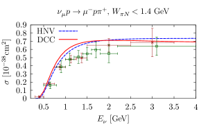
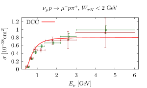
Figure 4: $\nu_{\mu}p\to\mu^{-}p\pi^{+}$ total cross section as a function of the neutrino energy. In the left panel a kinematical cut $W_{\pi N}<1.4\,\text{GeV}$ has been included. The corresponding experimental data has been taken from the reanalysis done in Ref. Rodrigues et al. (2016) of old ANL (crosses) and BNL (open squares) data, where the $W_{\pi N}<1.4\,\text{GeV}$ cut is also implemented. In the right panel a kinematical cut $W_{\pi N}<2\,\text{GeV}$ has been also applied to the theoretical calculation. The data has been taken from the reanalysis done in Ref. Wilkinson et al. (2014) of old ANL (crosses) and BNL (open squares) data, without any cut on $W_{\pi N}$.

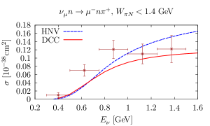
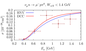
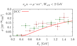
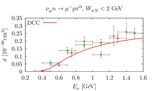
Figure 5: $\nu_{\mu}n\to\mu^{-}n\pi^{+}$ (left panels) and $\nu_{\mu}n\to\mu^{-}p\pi^{0}$ (right panels) total cross sections as a function of the neutrino energy. In the upper panels, the kinematical cut $W_{\pi N}<1.4\,\text{GeV}$ has been included in the data points, taken from the reanalysis of the experimental cross sections carried out in  Rodrigues et al. (2016), and both in the DCC and HNV theoretical predictions. For the DCC model, we also show the results for $W_{\pi N}<2\,\text{GeV}$ in the bottom panels. The corresponding experimental data has been taken also from the reanalysis carried out in Ref. Rodrigues et al. (2016) of the old ANL (crosses) and BNL (open squares) data, that does not incorporate any cut in the available phase space.

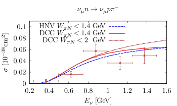
Figure 6: $\nu_{\mu}n\to\nu_{\mu}p\pi^{-}$ total cross section as a function of the neutrino energy. The corresponding experimental data has been taken from Ref. Derrick et al. (1980) where no kinematical cut was implemented. A kinematical cut $W_{\pi N}<1.4\,\text{GeV}$ has been, however, imposed for the HNV model (it has a moderate effect in this energy-range). We present the DCC results both with $W_{\pi N}<1.4\,\text{GeV}$ and $W_{\pi N}<2\,\text{GeV}$ cuts.

For a meaningful comparison between the HNV and DCC models we impose a $W_{\pi N}<1.4\,\text{GeV}$ cut. This is done to minimize the effect of higher order contributions in the chiral expansion not taken into account in the evaluation of the nonresonant background within the HNV model and, also, the possible unphysical behavior of the $\Delta$ amplitudes far from the $\Delta$ peak that would affect the HNV model (this unphysical behavior is discussed in Ref. González-Jiménez et al. (2017)). Besides, below this $W_{\pi N}$ cut, contributions from higher mass resonances, not taken into account in the HNV model, should be negligible.

For the $\nu_{\mu}p\to\mu^{-}p\pi^{+}$ channel we see that the DCC and HNV models produce similar results that lie above experimental data in the $1-2$ GeV neutrino energy region. To a lesser extent, this seems to also be the case for the DCC model evaluated with $W_{\pi N}<2\,\text{GeV}$ and shown in comparison with data in the right panel of Fig. 4. Note, however, that for the latter data no cut in $W_{\pi N}$ has been applied. For the $\nu_{\mu}n\to\mu^{-}n\pi^{+}$ channel the discrepancies between the two models are larger in the high neutrino energy region (see the top left panel of Fig. 5). The fact that the HNV model gives larger cross sections for that channel is a direct consequence of the $\Delta$ propagator modification in Eq. (9). The HNV predictions for this channel, without including the additional terms generated by the latter modification, can be seen (black dashed line) in the bottom panel of Fig. 3 in Ref. Hernández and Nieves (2017), and they were smaller than those obtained in the DCC model and shown here. For the $\nu_{\mu}n\to\mu^{-}p\pi^{0}$ and the NC $\nu_{\mu}p\to\nu_{\mu}p\pi^{-}$ channels, both the HNV and DCC models give again similar results that are in a good global agreement with data, as can be appreciated in the right upper panel of Fig. 5 and in Fig. 6.

Moving now to reactions induced by electron (anti-)neutrinos, in Figs. 7 and 8 we compare the HNV, SL and DCC total cross section predictions for all possible channels. We show results up to 2 GeV neutrino energy but imposing the cut $W_{\pi N}<1.4$ GeV. First, in Fig. 7, we display the CC channels, where we observe that the HNV and DCC models produce always larger cross section than the SL approach. This is mainly because the SL model uses the axial $N\to\Delta$ coupling predicted by a constituent quark model, while the DCC and HNV models use somewhat stronger couplings close to the PCAC prediction. The difference is particularly large in neutrino $n\pi^{+}$ and antineutrino $p\pi^{-}$ channels, for which the HNV cross sections are also significantly bigger than those predicted using the DCC model. As mentioned, this latter enhancement in the HNV predictions is due to the new contact term resulting from the $\Delta$ propagator modification of Eq. (9), and as discussed in Ref. Hernández and Nieves (2017), it seems to be supported by the old ANL and BNL bubble chamber $\nu_{\mu}n\to\mu^{-}n\pi^{+}$ data (see also upper left panel of Fig. 5). In these two channels, the strength of the crossed $\Delta$ term is enhanced by spin and isospin factors and it greatly cancels with the rest of the background. The modification of the $\Delta$ propagator significantly reduces the crossed $\Delta$ contribution, leading to a smaller cancellation with the background and, as net result, to an increase of the cross section. For the rest of the channels, the crossed $\Delta$ term is much smaller, and the DCC and HNV models produce similar results.

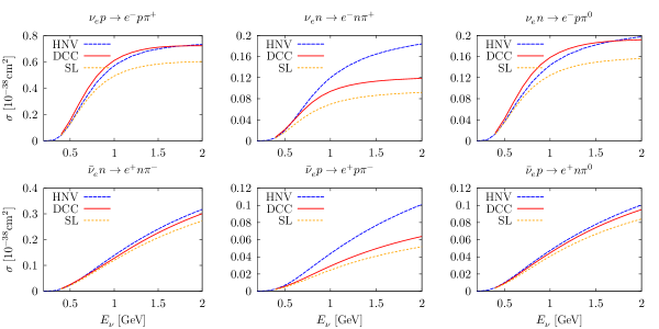
Figure 7: CC total cross sections as a function of the neutrino energy from different theoretical models. A kinematical cut $W_{\pi N}<1.4\,\text{GeV}$ on the final pion-nucleon invariant mass has been included.

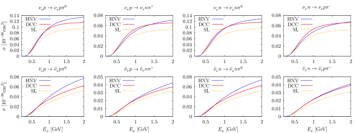
Figure 8: NC total cross sections as a function of the neutrino energy from different theoretical models. A kinematical cut $W_{\pi N}<1.4\,\text{GeV}$ on the final pion-nucleon invariant mass has been included.

Next in Fig. 8 we compare the results for the NC channels. The pattern is similar to that outlined above for the CC cross sections. DCC and HNV predictions agree reasonably well in general, while those obtained from the SL model are systematically lower for the reason mentioned in the previous paragraph. Here the modification in the $\Delta$ propagator of Eq. (9) implemented in the HNV model produces significantly smaller effects, because the isovector contribution to the amplitudes in all NC channels always involves both the $p\pi^{+}$ and $n\pi^{+}$ CC amplitudes, and there are no NC channels determined only by the latter of the two Hernández et al. (2007a).

IV.2 Differential cross sections

In Figs. 9 and 10, we now show CC and NC $d\sigma/(dQ^{2}dW_{\pi N})$ differential cross sections as a function of $W_{\pi N}$, for fixed $E_{\nu}=1\,\text{GeV}$ and $Q^{2}=0.1\,\text{GeV}^{2}/c^{2}$ values. The $Q^{2}$ value is in the range where the $d\sigma/dQ^{2}$ differential cross section is maximum. Very similar results (not shown) are obtained when $Q^{2}$ is varied in the interval $(0.05,0.15)\,\text{GeV}^{2}/c^{2}$.

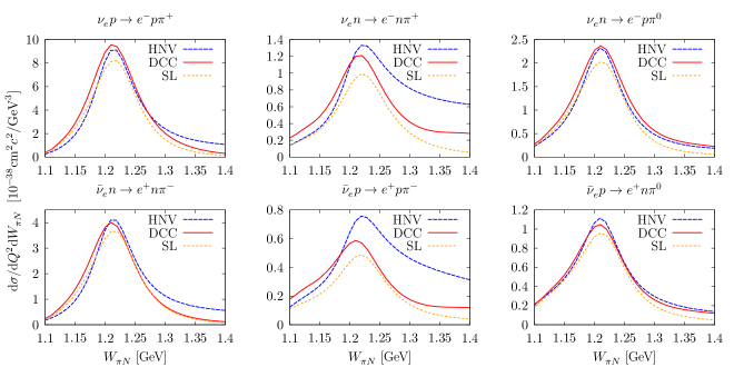
Figure 9: CC–$d\sigma/(dQ^{2}dW_{\pi N})$ differential cross sections as a function of $W_{\pi N}$, for fixed $E_{\nu}=1\,\text{GeV}$ and $Q^{2}=0.1\,\text{GeV}^{2}/c^{2}$.

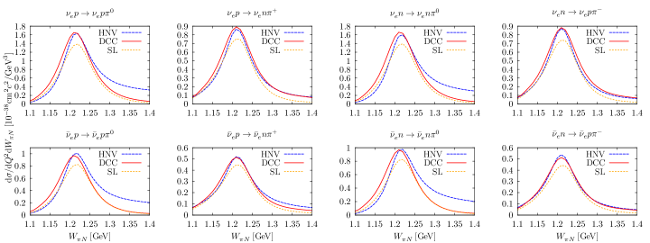
Figure 10: NC–$d\sigma/(dQ^{2}dW_{\pi N})$ differential cross sections as a function of $W_{\pi N}$, for fixed $E_{\nu}=1\,\text{GeV}$ and $Q^{2}=0.1\,\text{GeV}^{2}/c^{2}$.

All the distributions show the characteristic peak at the $\Delta$ pole. Apart from the differences in normalization, stemming from different total cross section predictions, we see that, in general, the SL and DCC models show more strength at lower $W_{\pi N}$ values, whereas the opposite happens for the HNV model. Again, this is more pronounced for the $\nu_{e}n\to e^{-}n\pi^{+}$ and $\bar{\nu}_{e}p\to e^{+}p\pi^{-}$ channels where the effects of the changes in the $\Delta$ propagator in Eq. (9) are more relevant. Nevertheless, and with the exception of these two latter reactions, we observe a reasonable agreement between the HNV and DCC models, in spite of the relative simplicity of the former as compared to the latter.

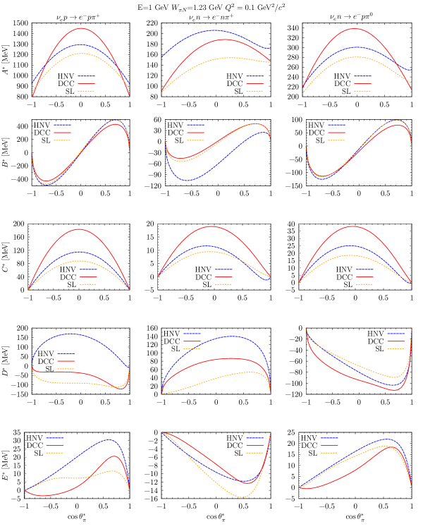
Figure 11: CC-neutrino $A^{*},B^{*},C^{*},D^{*}$ and $E^{*}$ structure functions, as defined in Eq. (35), represented as a function of $\cos\theta^{*}_{\pi}$ for fixed $E_{\nu}=1\,\text{GeV}$, $W_{\pi N}=1.23\,\text{GeV}$ and $Q^{2}=0.1\,\text{GeV}^{2}/c^{2}$.

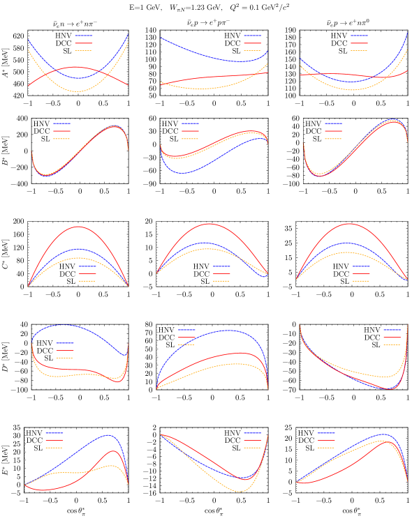
Figure 12: Same as Fig. 11 for CC-antineutrino reactions.

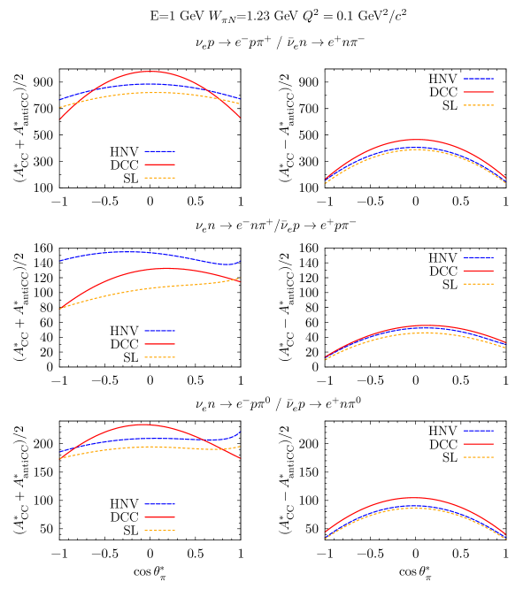
Figure 13: Semi-sums and semi-differences (in MeV units) of the neutrino and antineutrino $A^{*}$ structure functions displayed in Figs. 11 and 12.

Further fixing $W_{\pi N}=1.23\,\text{GeV}$, we show, in Figs. 11 (neutrinos) and 12 (antineutrinos), the $\cos\theta_{\pi}^{*}$ dependence of the $A^{*},B^{*},C^{*},D^{*}$ and $E^{*}$ CC structure functions introduced in Eq. (35). Some gross features of the shapes of these functions can be understood from the expressions given in the latter set of equations, bearing in mind that not only the second but also the first spatial components of $q^{*}$ and $p^{*}$ are zero, and that only $\hat{R}^{-1}k^{*}_{\pi}$ has a non-vanishing $X^{*}$ component, which is proportional to $\sin\theta_{\pi}^{*}$. Thus, we immediately see that $C^{*}$ and $E^{*}$ must be proportional to $\sin^{2}\theta_{\pi}^{*}$, since $(\widetilde{W}_{11}^{(s)}-\widetilde{W}_{22}^{(s)})$ and $\widetilde{W}_{12}^{(s)}$ are necessarily proportional to the square of $[\hat{R}^{-1}k^{*}_{\pi}]_{1}$. In addition, there might exist some additional dependence on $\theta_{\pi}^{*}$, because all the nucleon structure responses could be a function of the Lorentz scalar $q^{*}\cdot k^{*}_{\pi}$. These corrections look small for $C^{*}$ and more sizable for $E^{*}$, for which the DCC model, for example, predicts a change of sign in the $\nu_{e}p\to e^{-}p\pi^{+}$ and $\bar{\nu}_{e}n\to e^{+}n\pi^{-}$ channels. If one uses a multipole expansion of the hadronic amplitude, the deviation of $E^{*}$ from a pure $\sin^{2}\theta_{\pi}^{*}$ dependence originates from the interference with multipoles corresponding to a pion orbital angular momentum higher than one Sato and Lee (2009); Adler (1968).

Using the same type of argument, one can also factorize the $\sin\theta_{\pi}^{*}$ function in $B^{*}$ and $D^{*}$, which explains why these structure functions vanish at the extremes ($\cos\theta_{\pi}^{*}=\pm 1$). The additional $\theta_{\pi}^{*}$ dependencies, generated by $q^{*}\cdot k^{*}_{\pi}$ and by some other tensor terms in $B^{*}$ and $D^{*}$, give rise to large deviations from the $\sin\theta_{\pi}^{*}$ shape for these response functions.

Let us focus now on the neutrino processes. For the $\nu_{e}n\to e^{-}p\pi^{0}$ and $\nu_{e}n\to e^{-}n\pi^{+}$ channels, the three models produce structure functions with a similar shape. For the $\nu_{e}p\to e^{-}p\pi^{+}$, the $D^{*}$ structure function, and to a lesser extent the $E^{*}$ structure function, show larger differences in shape. These are precisely the two PV contributions to the differential cross section. As discussed in Sec. III.2.1, PV terms in the hadronic tensor derive from the interference between different contributions to the hadronic current that are not relatively real. The origin of these discrepancies should be found in the different pattern of relative phases in the three models. As seen from Eqs. (57) and (59), $D^{*}$ and $E^{*}$ are sensitive to the difference in phase of the multipole amplitudes. Below the two-pion production threshold, Watson theorem tells us that those phases are determined by the corresponding $\pi N$ phase shifts. The latter requirement is fully satisfied by the DCC and SL models, whereas this is not true for the HNV model where only a partial unitarization of the $P_{33}$ amplitude is implemented through the use of the Olsson phases. In the case of the $E^{*}$ structure function for the $\nu p\rightarrow e^{-}\pi^{+}p$ reaction, and keeping only $s$ and $p$ pion partial waves, one can explicitly observe that its value is given by the interference between the $P_{33}$ (dominated by the $\Delta$) and the $P_{31}$ (non-resonant) amplitudes

$$E^{*}\propto\sin^{2}\theta_{\pi}\sin(\delta_{P_{33}}-\delta_{P_{31}})[|M_{1+}^{V}||E_{1-}^{A}|+|M_{1-}^{V}|(4|M_{1+}^{A}|+2|E_{1+}^{A}|)].$$ (60)

Hypothetical future measurements of these structure functions might serve to further constrain the pion production models. Let us notice, however, that for the $\nu_{e}p\to e^{-}p\pi^{+}$ channel the magnitude of $D^{*}$ and $E^{*}$ is much smaller than $A^{*}$, getting at most $10\%$ of its value, whereas for the other two channels it reaches $\sim 30\%$.

For all structure functions, the various predictions differ not only in shape but also in size. This shows how demanding the test carried out in this work is. This is even more evident when the antineutrino structure functions, shown in Fig. 12, are examined. Isospin symmetry Hernández et al. (2007a) implies that the hadron tensors of the $\nu_{e}p\to e^{-}p\pi^{+}$ and $\bar{\nu}_{e}n\to e^{+}n\pi^{-}$ reactions are equal. The same happens for the $\nu_{e}n\to e^{-}n\pi^{+}$ and $\bar{\nu}_{e}p\to e^{+}p\pi^{-}$ processes, and for the $\nu_{e}n\to e^{-}p\pi^{0}$ and $\bar{\nu}_{e}p\to e^{+}n\pi^{0}$ processes. Therefore, the structure functions depicted in the first, second and third columns of Figs. 11 (neutrino) and  12 (antineutrino) should differ only in the terms proportional to the antisymmetric part of the lepton tensor, that changes sign. From the explicit expressions given in Eqs. (35), we immediately realize that neutrino and antineutrino $C^{*}$ and $E^{*}$ structure functions are identical, when looking at the appropriate channels. For the $A^{*}$ response function one sees significant differences between the DCC and HNV predictions for the antineutrino case. Thus, for instance in the $\bar{\nu}_{e}n\to e^{+}n\pi^{-}$ channel, we see that, compared to the HNV and SL models, the DCC model predicts a different shape, in contrast to the situation discussed above for the related neutrino $\nu_{e}p\to e^{-}p\pi^{+}$ channel. For the antineutrino reaction, the first two approaches lead to concave-up profiles, as a function of $\cos\theta^{*}_{\pi}$, while the latter one gives rise to a concave-down shape. However, DCC and HNV integrated $A^{*}$ structure functions differ by less than 5%, as can be inferred from the $d\sigma/dQ^{2}dW_{\pi N}$ differential cross sections depicted in the left bottom panel of Fig. 9. To shed light on this different behavior, we show in Fig. 13 the symmetric and antisymmetric contributions  to $A^{*}$ for the $\nu_{e}p\to e^{-}p\pi^{+}/\bar{\nu}_{e}n\to e^{+}n\pi^{-}$ (first row), $\nu_{e}n\to e^{-}n\pi^{+}/\bar{\nu}_{e}p\to e^{+}p\pi^{-}$ (second row) and $\nu_{e}n\to e^{-}p\pi^{0}/\bar{\nu}_{e}p\to e^{+}n\pi^{0}$ (third row) isospin related channels, at $W_{\pi N}=1.23\,\text{GeV}$ and $Q^{2}=0.1\,\text{GeV}^{2}/c^{2}$ as in Figs. 11 and  12. DCC antisymmetric contributions to $A^{*}$ are larger than those obtained within the HNV and SL models. If we focus on the results found for $\nu_{e}p\to e^{-}p\pi^{+}/\bar{\nu}_{e}n\to e^{+}n\pi^{-}$, we see that all models predict similar $\cos\theta^{*}_{\pi}$ shapes (concave-down) for both the symmetric and antisymmetric terms of $A^{*}$, but when they are subtracted to obtain the antineutrino structure functions, they give rise to concave-up shapes in the HNV and SL approaches. This illustrates the importance of carrying out a thorough test of the different model results at the level of outgoing pion angular distributions, going beyond comparisons done for partially integrated cross sections, where the differences tend to cancel. In addition, we can conclude from Fig. 13 that the inclusion in the HNV model of a local term, induced by the $\Delta$ propagator modification discussed in Eq. (9), produces visible effects in the symmetric contribution to $A^{*}$ in the $\nu_{e}n\to e^{-}n\pi^{+}$ and $\bar{\nu}_{e}p\to e^{+}p\pi^{-}$ reactions.

Returning to the discussion of Figs. 11 and 12, we see that, in general, $|D^{*}|$ is greater than $|E^{*}|$, and thus PV effects are dominated by the $\sin\phi^{*}_{\pi}$ dependence of the differential cross section. Comparing the relative sizes of $A^{*}$ and $|D^{*}|$, we expect the largest parity violations in the $\nu_{e}n\to e^{-}n\pi^{+}$, $\bar{\nu}_{e}p\to e^{+}p\pi^{-}$, $\nu_{e}n\to e^{-}p\pi^{0}$ and $\bar{\nu}_{e}p\to e^{+}n\pi^{0}$ reactions, while the smallest ones should occur in the isospin 3/2 $\nu_{e}p\to e^{-}p\pi^{+}$ and $\bar{\nu}_{e}n\to e^{+}n\pi^{-}$ channels, that are dominated by the direct $\Delta$ mechanism. In addition, in this latter case, we observe that PV effects are greatly reduced for $\bar{\nu}_{e}n\to e^{+}n\pi^{-}$, since the relative size of the $|D^{*}|/A^{*}$ ratio for this reaction is significantly smaller than for the isospin related one $\nu_{e}p\to e^{-}p\pi^{+}$.

All of the above features are visible in the neutrino and antineutrino CC $d\sigma/(dQ^{2}dW_{\pi N}d\Omega^{*}_{\pi})$ differential cross sections that are displayed as contour plots in Figs. 14 and 15 for the DCC and HNV models. They are given as a function of $\phi_{\pi}^{*}$ and $\theta_{\pi}^{*}$, and have been evaluated for fixed $E_{\nu}=1\,\text{GeV}$, $Q^{2}=0.1\,\text{GeV}^{2}/c^{2}$ and $W_{\pi N}=1.23\,\text{GeV}$ values.

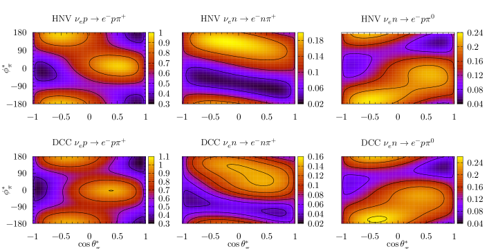
Figure 14: Neutrino CC–$d\sigma/(dQ^{2}dW_{\pi N}d\Omega^{*}_{\pi})$ differential cross section in units of $10^{-38}\text{cm}^{2}c^{2}/\text{GeV}^{3}$, as a function of $\phi_{\pi}^{*}$ and $\theta_{\pi}^{*}$, evaluated for fixed $E_{\nu}=1\,\text{GeV}$, $Q^{2}=0.1\,\text{GeV}^{2}/c^{2}$ and $W_{\pi N}=1.23\,\text{GeV}$ values.

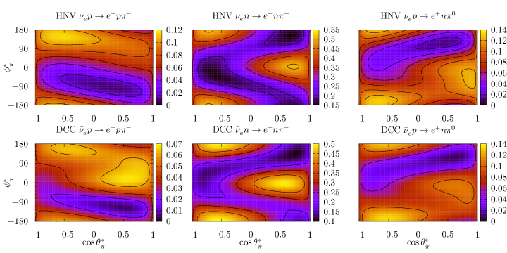
Figure 15: The same as in Fig. 14 for antineutrino CC–$d\sigma/(dQ^{2}dW_{\pi N}d\Omega^{*}_{\pi})$.

Despite the differences, we find a good qualitative agreement between the two models that predict similar regions where the pion angular distribution reaches its maximum and minimum. The same applies to the case of NC processes that are shown in Figs. 16 and 17. Note that the $n\pi^{0}$ and $p\pi^{0}$ NC reactions are driven by the same isovector amplitude, and they differ only in the sign of the interference of the latter with the isoscalar part of the amplitude, which is also the same in both reactions Hernández et al. (2007a). This is the reason why, as long as these processes are largely dominated by the isovector excitation of the $\Delta-$resonance, the cross sections are similar. The same occurs in the case of the $p\pi^{-}$ and $n\pi^{+}$ NC reactions. Let us note, in addition, that the isoscalar contributions for these two latter processes are a factor of two bigger than for the two previous NC reactions where neutral pions are produced Hernández et al. (2007a).

Since in Figs. 14–17 we take $\phi^{*}_{\pi}$ in the interval $[-\pi,\pi]$, parity violation for $d\sigma/(dQ^{2}dW_{\pi N}d\Omega^{*}_{\pi})$ is clearly seen in most cases by the lack of reflection symmetry with respect to the $\phi^{*}_{\pi}=0$ line. It is significant for CC $\nu_{e}$ scattering off neutron ($\bar{\nu}_{e}$ off proton), where the direct $\Delta$ excitation term is not so dominant, and for neutrino NC reactions producing charged pions. It means that for these channels, the $D^{*}$ and/or $E^{*}$ terms should have sizes comparable in magnitude to those of the $A^{*}$, $B^{*}$ and $C^{*}$ parity-conserving structure functions. Parity violation is less prominent for the antineutrino NC processes for which both models predict rather symmetric distributions. By looking at the NC channels with a final charged pion, one sees a transition between a clear asymmetry for neutrino reactions to a fairly symmetric distribution for the antineutrino case. Since the NC hadronic tensor is the same for neutrinos and antineutrinos, the different behavior seen in the figures originates from the change of sign of the antisymmetric part of the leptonic tensor. From the general discussion in Sec. III.2.1, there are two types of PV terms in $D^{*}$, that correspond to those induced by the antisymmetric ${\cal\widetilde{H}}^{\mu\nu\,(a)}_{VV+AA}$ and the symmetric ${\cal\widetilde{H}}^{\mu\nu\,(s)}_{VA+AV}$ nucleon tensors, discussed in Eqs. (46) and (49), respectively. When contracted with the leptonic tensor, these two contributions tend to cancel each other for the NC antineutrino case, implying that both PV contributions must be similar in magnitude for NC processes. A similar behavior is seen in the HNV model for NC channels with a final $\pi^{0}$. For this latter case, the DCC model produces almost perfect symmetric distributions for antineutrinos, and though some asymmetries can be seen for neutrinos, they are not as pronounced as in the HNV case.

Another feature worth noticing, easily deduced from Figs. 14-17, is that the $\phi^{*}_{\pi}$ dependence of the differential cross section is very different for $\cos\theta_{\pi}^{*}<0$ and $\cos\theta_{\pi}^{*}>0$.

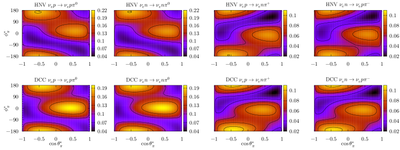
Figure 16: The same as in Fig. 14 for neutrino NC–$d\sigma/(dQ^{2}dW_{\pi N}d\Omega^{*}_{\pi})$.

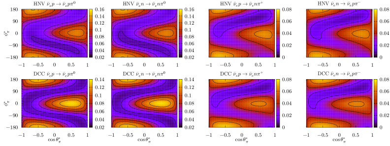
Figure 17: The same as in Fig. 14 for antineutrino NC–$d\sigma/(dQ^{2}dW_{\pi N}d\Omega^{*}_{\pi})$,

In Fig. 18 we show now the $d\sigma/d\Omega^{*}_{\pi}$ differential cross section for the $\nu_{e}p\to e^{-}p\pi^{+},\nu_{e}n\to e^{-}n\pi^{+},\bar{\nu}_{e}n\to e^{+}n\pi^{-}$ and $\nu_{e}p\to\nu_{e}p\pi^{0}$ channels evaluated at $E_{\nu}=1\,\text{GeV}$ and with a cut $W_{\pi N}<1.4$ GeV. Parity violation is seen in both models in the case of the $\nu_{e}n\to e^{-}n\pi^{+}$ reaction, while for $\nu_{e}p\to e^{-}p\pi^{+}$ and $\nu_{e}p\to\nu_{e}p\pi^{0}$ a PV pattern is only clearly appreciable in the HNV model. Both models predict very small PV effects in the case of the $\bar{\nu}_{e}n\to e^{+}n\pi^{-}$ reaction. The three latter processes are largely dominated by the excitation of the $\Delta$ and its subsequent $\pi N$ decay, and thus finding small PV signatures is not surprising. Moreover, we see once more that PV effects get substantially reduced in the antineutrino $\bar{\nu}_{e}n\to e^{+}n\pi^{-}$ reaction as compared to those found in the isospin related neutrino $\nu_{e}p\to e^{-}p\pi^{+}$ process (see discussion of Figs. 11 and 12).

In any case, all distributions show a clear anisotropy. This means that using an isotropic distribution for the pions in the center of mass of the final pion-nucleon system, as assumed in some Monte Carlo event generators, is not supported by the results in Fig. 18. Moreover, different channels have different angular distributions.

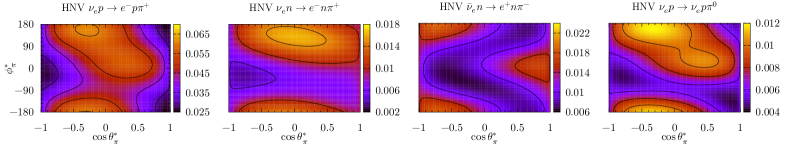
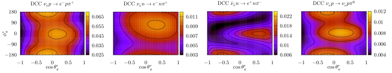
Figure 18: $d\sigma/d\Omega^{*}_{\pi}$ differential cross section in units of $10^{-38}\text{cm}^{2}$, as a function of $\phi_{\pi}^{*}$ and $\theta_{\pi}^{*}$, evaluated at $E_{\nu}=1\,\text{GeV}$ and with a $W_{\pi N}<1.4$ GeV cut.

In Figs. 19 and 20 we display the $d\sigma/d\cos\theta^{*}_{\pi}$ and $d\sigma/d\phi^{*}_{\pi}$ differential cross sections, respectively, for the same channels and incoming neutrino energy as the ones shown in Fig. 18, and with the same $W_{\pi N}<1.4$ GeV cut applied. They are not flat and again different channels show different behaviors. Looking at the $d\sigma/d\cos\theta^{*}_{\pi}$ differential cross section one sees that the two models predict distributions similar in shape and size for the $\nu_{e}p\to e^{-}p\pi^{+}$ and $\nu_{e}p\to\nu_{e}p\pi^{0}$ channels. The discrepancies are more visible for $\bar{\nu}_{e}n\to e^{+}n\pi^{-}$. Note that isospin invariance guarantees that the hadron tensors of the $\nu_{e}p\to e^{-}p\pi^{+}$ and the $\bar{\nu}_{e}n\to e^{+}n\pi^{-}$ processes should be identical, and therefore the differences in the cross sections should only be produced by the change of sign of the interference between vector and axial contributions. The largest differences between DCC and HNV predictions are found, however, for the $\nu_{e}n\to e^{-}n\pi^{+}$ channel, as we have already seen in Figs. 7, 9 and 11. They are mainly due to the inclusion in the HNV model of a local term induced by the $\Delta$ propagator modification discussed in Eq. (9). This term notably improves the description of the $\nu_{\mu}n\to\mu^{-}n\pi^{+}$ total ANL cross section data Hernández and Nieves (2017) (see also Fig. 5 here).

As for the $d\sigma/d\phi^{*}_{\pi}$ differential cross section, first we observe that the distributions are not symmetric around $\phi^{*}_{\pi}=\pi$, implying certain violations of parity, which are quite significant for the $\nu_{e}n\to e^{-}n\pi^{+}$ reaction. Both, the HNV and the DCC models predict more pions to be produced above the scattering plane, i. e. $\phi^{*}_{\pi}\in[0,\pi[$, for the $\nu_{\mu}n\to\mu^{-}n\pi^{+}$ and $\nu_{e}p\to\nu_{e}p\pi^{0}$ reactions. The asymmetry for the $\nu_{e}p\to e^{-}p\pi^{+}$ channel is predicted to be small in both models but with a different sign. For $\bar{\nu}_{e}n\to e^{+}n\pi^{-}$, PV effects are larger in the DCC predictions than in the HNV ones, since in the former, the number of pions produced above the scattering plane is clearly smaller than that below that plane.

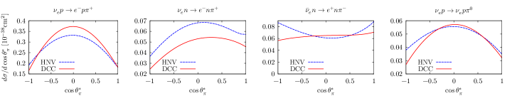
Figure 19: $d\sigma/d\cos\theta^{*}_{\pi}$ differential cross section in units of $10^{-38}\text{cm}^{2}$ for $E_{\nu}=1\,\text{GeV}$, and with a $W_{\pi N}<1.4$ GeV cut.

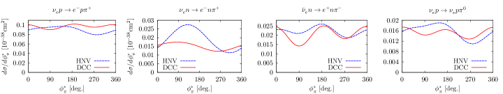
Figure 20: $d\sigma/d\phi^{*}_{\pi}$ differential cross section in units of $10^{-38}\text{cm}^{2}$ for $E_{\nu}=1\,\text{GeV}$, and with a $W_{\pi N}<1.4$ GeV cut.

Finally, in Fig. 21, we make a shape-only comparison of our theoretical results for the $d\sigma/d\cos\theta^{*}_{\pi}$ and $d\sigma/d\phi^{*}_{\pi}$ differential cross sections for the $\nu_{\mu}p\to\mu^{-}p\pi^{+}$ reaction with unnormalized ANL Radecky et al. (1982) and BNL Kitagaki et al. (1986) old bubble chamber data. Both in the data and in the theoretical calculations, the cut $W_{\pi N}<1.4$ GeV in the final pion-nucleon invariant mass is imposed, and the theoretical distributions have been obtained averaging over the neutrino flux for neutrino energies in the $[0.5,6]$ GeV interval. The theoretical results have been area-normalized to the data. Predictions from two previous versions of the HNV model are also shown to elucidate how the local terms discussed in Eq. (9) Hernández and Nieves (2017) and the implementation of Watson theorem Alvarez-Ruso et al. (2016) affect this channel, dominated by the direct excitation of the $\Delta$ resonance.

All the models give similar predictions for the flux averaged $d\sigma/d\cos\theta^{*}_{\pi}$ differential cross section, and show a good agreement with BNL data. This means that the corrections for the HNV model proposed in Refs. Hernández and Nieves (2017) and Alvarez-Ruso et al. (2016) have little effect not only on the integrated, but also on the $\cos\theta^{*}_{\pi}$ differential cross section for the $\nu_{\mu}p\to\mu^{-}p\pi^{+}$ reaction, that we remind again, it is largely dominated by the direct $\Delta$ excitation term. For the flux averaged $d\sigma/d\phi^{*}_{\pi}$ differential cross section, the DCC model exhibits a global better agreement with data. As expected, the PV effects, both in the data and theoretical predictions, are small, being largely obscured by the uncertainties in the experimental distribution. HNV models predict larger asymmetries, though still small in absolute value, around 10% maximum. On the other hand, the inclusion of the local terms discussed in Eq. (9) Hernández and Nieves (2017) increases the differences with the DCC results, and it also seems that the induced changes in the shape of the distribution do not receive data support.

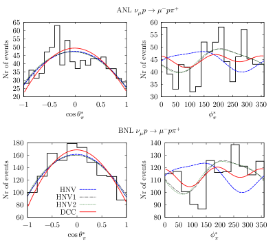
Figure 21: Shape comparison of the theoretical $d\sigma/d\cos\theta^{*}_{\pi}$ (left panels) and $d\sigma/d\phi^{*}_{\pi}$ (right panels) differential cross sections with unnormalized ANL Radecky et al. (1982) and BNL Kitagaki et al. (1986) data. A cut $W_{\pi N}<1.4$ GeV, in the final pion-nucleon invariant mass is imposed in both data and the theoretical results. Theoretical results have been obtained averaging over the neutrino flux for neutrino energies in the $[0.5,6]$ GeV interval, setting their overall size to reproduce the areas under the experimental data. Predictions from two previous versions of the HNV model are also displayed: HNV1 stands for the HNV model without the $\Delta$ propagator modification of Eq. (9), while to compute the HNV2 results, the implementation of Watson theorem has been further suppressed.

V Study of pion electroproduction as a test of the vector part of the DCC, SL and HNV models

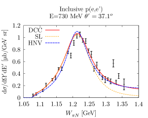
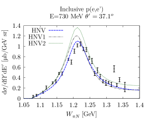
Figure 22: Inclusive $d\sigma/(d\Omega^{\prime}dE^{\prime})$ cross section off a proton (sum of the differential distributions for the $e^{-}p\to e^{-}p\pi^{0}$ and $e^{-}p\to e^{-}n\pi^{+}$ reactions), as a function of the invariant mass $W_{\pi N}$ and for fixed $\theta^{\prime}=37.1^{\rm o}$. The four-momentum transfer square $Q^{2}$ varies in the interval $[0.18,0.04]\,\text{GeV}^{2}/c^{2}$, when $W_{\pi N}\in[1,1.4]$ GeV. Data taken from Ref. O’Connell et al. (1984). In the right panel, predictions from the HNV and two previous versions of that model are displayed: HNV1 stands for the HNV model without the $\Delta$ propagator modification of Eq. (9), while to compute the HNV2 results, the implementation of Watson theorem has been further suppressed.

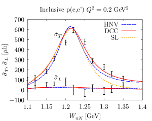
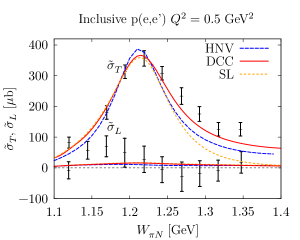
Figure 23: Data and theoretical predictions for the $\tilde{\sigma}_{T}=\int\sigma_{T}d\Omega_{\pi}^{*}$ and $\tilde{\sigma}_{L}=\int\sigma_{L}d\Omega_{\pi}^{*}$ inclusive cross sections off protons ($p\pi^{0}+n\pi^{+}$), as a function of the $\pi N$ invariant mass, and for two fixed values of $Q^{2}=0.2\ \rm GeV^{2}$ (left panel) and $Q^{2}=0.5\rm GeV^{2}$ (right panel). Data taken from Ref. Baetzner et al. (1972).

Pion electroproduction provides a testing ground for the vector part of the pion production models. We do not aim here to perform an exhaustive comparison with the abundant data that are available. In fact, such a test has already been done for the SL and DCC models Kamano et al. (2013); Sato and Lee (1996, 2001). Here we just want to show the observables which are described in a similar way by the HNV, SL and DCC models, as well as those that differ, trying to understand the origin of the discrepancies. This should help us to better understand the differences observed in the weak pion production.

In Sec. IV we have compared the three models for CC and NC reactions induced by neutrinos in the vicinity of the $\Delta$ peak, and for a relatively low $Q^{2}$ value in the region where the $d\sigma/dQ^{2}$ cross section is maximum. For a similar kinematical setup, we now show results for pion electroproduction differential cross sections integrated over the outgoing pion variables. In Fig. 22, we show results for the $d\sigma/(dE^{\prime}d\Omega^{\prime})$ differential cross section off protons evaluated for an incoming electron energy of $E=0.73\,$ GeV and for fixed $\theta^{\prime}=37.1^{\rm o}$. The results are plotted as a function of $W_{\pi N}$ and we compare them with experimental data taken from Ref. O’Connell et al. (1984). In its left panel we see that the HNV and DCC models give very similar predictions which, in turn, are in a good agreement with the data. The HNV model predicts less strength for low $W_{\pi N}$, something that has also been observed for the neutrino induced reactions, see Figs. 9 and 10. At the $\Delta$ resonance peak and below, the SL and DCC give very similar results, since the $N\to\Delta$ vector form factors were adjusted to reproduce the pion electroproduction data. Above resonance, the SL model gives smaller cross sections. In the case of neutrino cross sections, the differences seen between the SL and the DCC models are, however, mainly due to the difference in strength in the axial current in those two models. In the right panel we show the predictions of the HNV model when the modification of the $\Delta$ propagator in Eq. (9) is not taken into account (HNV1), and when we further suppress the implementation of Watson theorem (HNV2). One sees that the results significantly improve when going from HNV2 to HNV1 and from HNV1 to the full HNV model, leading to an excellent description of the experimental distribution. This is particularly reassuring because, though the HNV model uses vector form-factors that have been in principle fitted to data, its latest refinement Hernández and Nieves (2017) (modification of the $\Delta$ propagator, motivated by the use of the so called consistent couplings Pascalutsa (2001)) was derived only from neutrino pion production data. Note that the final $p\pi^{0}$ and $n\pi^{+}$ states in the electron induced reactions are not purely isospin 3/2 states, and thus they receive sizable contributions from non-resonant mechanisms, in particular from the $\Delta$ crossed term which is corrected by the use of consistent couplings.

For electrons we have access to very precise experimental measurements of the pion angular distributions. It is common to write the differential cross section as (see Eq. (112))

$$\frac{d\sigma_{em}}{d\Omega^{\prime}dE^{\prime}d\Omega^{*}_{\pi}}=\Gamma_{em}\Big{\{}\sigma_{T}+\varepsilon\,\sigma_{L}+\sqrt{2\varepsilon(1+\varepsilon)}\ \sigma_{LT}\,\cos\phi^{*}_{\pi}+h\sqrt{2\varepsilon(1-\varepsilon)}\ \sigma_{LT^{\prime}}\,\sin\phi^{*}_{\pi}+\varepsilon\,\sigma_{TT}\,\cos 2\phi^{*}_{\pi}\Big{\}}$$ (62)

where the different quantities have been introduced in Appendix D. It is a valid expression when both electrons are ultrarelativistic and the initial electron is polarized with well defined helicity $h$. As also mentioned in Subsec. III.2 and the Appendix D, the presence of the $\sin\phi^{*}_{\pi}$ term does not imply parity violation in this case, since the helicity also changes sign under parity. It is straightforward to see a direct correspondence of the terms $\sigma_{T}+\varepsilon\,\sigma_{L}$, $\sigma_{LT}$, $\sigma_{TT}$ and $\sigma_{LT^{\prime}}$ and the $A^{*}$, $B^{*}$, $C^{*}$ and $D^{*}$ structure functions introduced for neutrinos in Eq. (35).

After integrating over $\Omega_{\pi}^{*}$, only the $\sigma_{T}$ and $\sigma_{L}$ terms contribute to the $d\sigma_{em}/(d\Omega^{\prime}dE^{\prime})$ differential cross section. These partially integrated distributions

$$\tilde{\sigma}_{T}=\int\sigma_{T}d\Omega_{\pi}^{*}\ ,\ \ \tilde{\sigma}_{L}=\int\sigma_{L}d\Omega_{\pi}^{*}$$

have been measured for various values of $Q^{2}$ and $W_{\pi N}$. In Fig. 23, we present the predictions for $\tilde{\sigma}_{T,L}$ obtained from the DCC, SL and HNV models and they are compared to the data of Ref. Baetzner et al. (1972). Not much can be said about the accuracy of the predictions for $\tilde{\sigma}_{L}$ because of the large experimental uncertainties. For $\tilde{\sigma}_{T}$, which largely dominates over $\tilde{\sigma}_{L}$, we find an acceptable description of the data, and we observe a similar behavior as in the case of $d\sigma_{em}/(d\Omega^{\prime}dE^{\prime})$ presented in Fig. 22: the HNV predicts less strength below the $\Delta$ peak, while the SL model underestimates the experimental points above it.

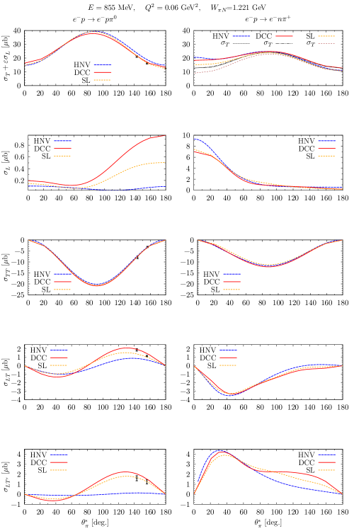
Figure 24: Comparison of the $\sigma_{T}+\varepsilon\,\sigma_{L}$, $\sigma_{L}$, $\sigma_{TT}$, $\sigma_{LT}$, $\sigma_{LT^{\prime}}$ pion polar angular distributions obtained using the DCC, SL and HNV models for the $e^{-}p\rightarrow e^{-}p\pi^{0}$ (left panels) and $e^{-}p\rightarrow e^{-}n\pi^{+}$ (right panels) channels. The kinematics correspond to $Q^{2}=0.06\ \text{GeV}^{2}/c^{2}$, $W_{\pi N}=1.221$ GeV and an incoming electron energy of 0.855 GeV. For $e^{-}p\rightarrow e^{-}p\pi^{0}$, the $\sigma_{L}$ contribution is negligible so that $\sigma_{T}+\varepsilon\,\sigma_{L}\approx\sigma_{T}$, while for $e^{-}p\rightarrow e^{-}n\pi^{+}$ we also show $\sigma_{T}$ in the first panel. Data from Ref. Stave et al. (2006) are available only for the $p\pi^{0}$ channel.

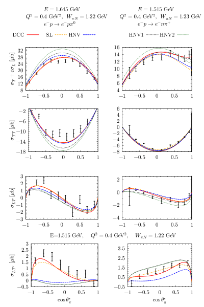
Figure 25: Comparison of the $\sigma_{T}+\varepsilon\,\sigma_{L}$, $\sigma_{TT}$ and $\sigma_{LT}$ pion polar angular distributions obtained using the DCC, SL and HNV models for $e^{-}p\rightarrow e^{-}p\pi^{0}$ (left panels) and $e^{-}p\rightarrow e^{-}n\pi^{+}$ (right panels) at $Q^{2}=0.4\,\text{GeV}^{2}/c^{2}$ and $W_{\pi N}=1.22$ GeV or $1.23$ GeV, respectively. Data from Refs. Joo et al. (2002) and  Egiyan et al. (2006) for $e^{-}p\rightarrow e^{-}p\pi^{0}$ and $e^{-}p\rightarrow e^{-}n\pi^{+}$, respectively, are displayed as well. In the two bottom panels, we also show the $p\pi^{0}$ and $n\pi^{+}$ measurements of Refs. Joo et al. (2003) (left) and  Joo et al. (2005) (right) at $Q^{2}=0.4\,\text{GeV}^{2}/c^{2}$ and $W_{\pi N}=1.22$ GeV, together with the theoretical predictions, of the $\sigma_{LT^{\prime}}$ distribution. Finally in all panels, the HNV1 curves stand for the results obtained within the HNV model, when the propagator modification of Eq. (9) is not considered, while to obtain the HNV2 predictions, the implementation of Watson theorem is further suppressed.

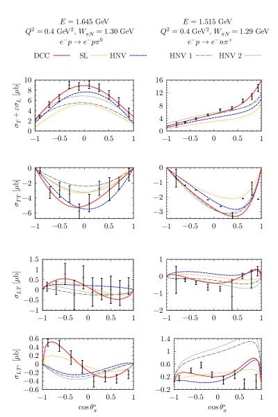
Figure 26: Same as Fig. 25 ($Q^{2}=0.4\,\text{GeV}^{2}/c^{2}$), but for higher $\pi N$ invariant masses, $W_{\pi N}=1.30$ GeV and $1.29$ GeV for $e^{-}p\rightarrow e^{-}p\pi^{0}$ and $e^{-}p\rightarrow e^{-}n\pi^{+}$, respectively.

In the following, we shall further compare the theoretical pion angular distributions for the $e^{-}p\rightarrow e^{-}p\pi^{0}$ and $e^{-}p\rightarrow e^{-}n\pi^{+}$ channels, for $W_{\pi N}$ invariant masses in the vicinity of the $\Delta$ peak and for two $Q^{2}$ values for which precise data are available. In Fig. 24, we show results for $W_{\pi N}=1.221$ GeV and a very low $Q^{2}=0.06\ \text{GeV}^{2}/c^{2}$ value and compare them to data taken from Ref. Stave et al. (2006). The latter correspond to the lowest $Q^{2}$ measurement of these observables that has been performed so far. They cover a small $\theta_{\pi}^{*}$ range, above $140^{\circ}$, and only for the $e^{-}p\rightarrow e^{-}p\pi^{0}$ channel. We show results from the three models, for both $p\pi^{0}$ and $n\pi^{+}$ final states, and the full $\theta_{\pi}^{*}$ range. For the $e^{-}p\rightarrow e^{-}n\pi^{+}$ channel (right panels in Fig. 24) all models give very similar results for all the structure functions. For $e^{-}p\rightarrow e^{-}p\pi^{0}$ (left panels in Fig. 24), the theoretical predictions differ for the transverse-longitudinal interference terms, $\sigma_{LT^{\prime}}$ and $\sigma_{LT}$, and also for the longitudinal $\sigma_{L}$ differential cross section. These contributions are much smaller than $\sigma_{T}$ ($\leq 5\%$), in particular $\sigma_{L}$, so that all models would predict similar $d\sigma/dQ^{2}dW_{\pi N}$ cross sections. As it has been discussed at the end of Sec. III.2.1, in the case of the HNV model, $\sigma_{LT^{\prime}}$ (or correspondingly the $D^{*}$ function for neutrinos) appears as a consequence of interference between the $\Delta P$ term and the background contributions (which have different phases mainly because of the nonzero imaginary part of the $\Delta$ propagator). Background terms in the $e^{-}p\rightarrow e^{-}p\pi^{0}$ channel are small within the HNV model (isospin symmetry forbids the CT and the PF contributions), and thus that interference is necessarily small. The situation is entirely different for the $e^{-}p\rightarrow e^{-}n\pi^{+}$ channel, for which the background contribution is sizable. This is the reason why the three models give very similar predictions in this case. By looking at Eq. (116), one realizes that $\sigma_{L}$, $\sigma_{LT}$ and $\sigma_{LT^{\prime}}$ depend on the third component of the hadronic electromagnetic current. The above discussion tells us that for the $e^{-}p\rightarrow e^{-}p\pi^{0}$ channel, this component may not be correct within the HNV model.

In a multipole language, the main features of the $\sigma_{LT^{\prime}}$ angular distribution in the $\Delta$ region can be understood using $s$ and $p$ wave pion production multipoles, as done for instance in Ref. Joo et al. (2005)

$$\sigma_{LT^{\prime}}\approx\frac{|\vec{k}^{*}_{\pi}|_{0}}{k_{\gamma}}\sqrt{\frac{Q^{2}}{|\vec{q}^{*}|^{2}}}\sin\theta^{*}_{\pi}({\cal A}+{\cal B}\cos\theta_{\pi}^{*}),$$ (63)

with

$${\cal A}={\rm Im}[S^{*}_{0+}(-M_{1+}+3E_{1+}+M_{1-})+(S_{1-}-2S_{1+})^{*}E_{0+}]\ \ ,\ \ {\cal B}=6{\rm Im}[S^{*}_{1-}E_{1+}+S^{*}_{1+}(E_{1+}-M_{1+}+M_{1-})],$$ (64)

and $k_{\gamma}$ defined in Appendix C. ${\cal A}$ comes from the interference between $s$ and $p$ wave multipoles while ${\cal B}$ is generated from the interference among $p$ wave multipoles. Since the direct Delta contributes only to $P_{33}$ multipoles, all with the same phase, $\sigma_{LT^{\prime}}$ is very sensitive to background contributions. In the DCC and SL models, the main contributions to ${\cal A}$ and ${\cal B}$ are respectively $-{\rm Im}[S^{*}_{0+}M_{1+}]$ and $-{\rm Im}[S^{*}_{1+}M_{1+}]$. The latter can only come from isospin 3/2 and isospin 1/2 interference and it changes sign when going from $\pi^{0}$ to $\pi^{+}$ production. This change of sign of ${\cal B}$ explains the difference in shape for $\sigma_{LT^{\prime}}$ seen when going from $\pi^{0}$ to $\pi^{+}$ production. It is also clear that the relative phases between the multipoles have to be well under control to get $\sigma_{LT^{\prime}}$ right. This is achieved in the DCC and SL models below the two-pion production threshold.

Next, we show $e^{-}p\rightarrow e^{-}p\pi^{0}$ and $e^{-}p\rightarrow e^{-}n\pi^{+}$ results evaluated at a higher $Q^{2}=0.4\ \text{GeV}^{2}/c^{2}$ value, and for $\pi N$ invariant masses located at the $\Delta$ peak (Fig. 25) or slightly above (Fig. 26). The three models give similar results in good agreement with data, with the exceptions of the SL $\sigma_{T}+\varepsilon\sigma_{L}$ and $\sigma_{TT}$ distributions above the $\Delta$, and the HNV $\sigma_{LT^{\prime}}$ structure function, particularly for the $e^{-}p\rightarrow e^{-}p\pi^{0}$ channel, for which the background contribution within the HNV model is small. We also show in these two figures results obtained when we eliminate from the HNV model the $\Delta$ propagator modification of Eq. (9), and when we further suppress the partial unitarization of the amplitudes, implemented by imposing Watson theorem for the multipoles dominated by the $\Delta$ resonance. In the $p\pi^{0}$ case, one sees a clear improvement in the $\sigma_{T}+\varepsilon\sigma_{L}$ and $\sigma_{TT}$ observables when going from HNV2 to HNV1 and from the latter to the full HNV calculation. For $\sigma_{LT}$ the quality of the data does not allow us to be very conclusive, while the three versions of the HNV model fail to reproduce the data of the small $\sigma_{LT^{\prime}}$. For the $n\pi^{+}$ reaction, though in general the modifications proposed in Refs. Alvarez-Ruso et al. (2016); Hernández and Nieves (2017) improve the global agreement with data, the effects are not as pronounced as those found in the $p\pi^{0}$ case.

The conclusion to be drawn from this comparison of electromagnetic results is that one needs a full unitarization procedure, like the one implemented in the complex DCC model in order to get a good reproduction of all scattering observables. Its effect seems to be crucial to explain the $\sigma_{LT}$ and $\sigma_{LT^{\prime}}$ data for the $e^{-}p\rightarrow e^{-}p\pi^{0}$ reaction, where background contributions are small. In the $e^{-}p\rightarrow e^{-}n\pi^{+}$ channel, the non-resonant contributions are much more important, and the simple HNV model predictions agree reasonably well with those obtained within the sophisticated DCC approach. All that notwithstanding, it is important to stress that the $\sigma_{L}$, $\sigma_{LT}$ and $\sigma_{LT^{\prime}}$ structure functions, where the HNV model shows larger discrepancies with the DCC results, are much smaller in magnitude than $\sigma_{T}$ and $\sigma_{TT}$ and thus their effects are not so relevant when looking at pion angular distributions. Besides, if one integrates on the outgoing pion $\phi_{\pi}^{*}$ variable, the contributions from $\sigma_{LT}$ and $\sigma_{LT^{\prime}}$ (and $\sigma_{TT}$) cancel exactly and the resulting differential cross section is governed by $\sigma_{T}+\varepsilon\sigma_{L}$ for which, both the HNV and DCC models give similar predictions.

VI Summary and conclusions

We have carried out a careful analysis of the pion angular dependence of the CC and NC neutrino and antineutrino pion production reaction off nucleons. We have shown that the possible dependencies on the azimuthal angle measured in the final pion-nucleon CM system are $1,\cos\phi^{*}_{\pi},\cos 2\phi^{*}_{\pi},\sin\phi^{*}_{\pi}$ and $\sin 2\phi^{*}_{\pi}$, and that the two latter ones give rise to parity violation and time-reversal odd correlations in the weak $d\sigma/(d\Omega^{\prime}dE^{\prime}d\Omega^{*}_{\pi})$ and $d\sigma/(dQ^{2}dW_{\pi N}d\Omega^{*}_{\pi})$ differential cross sections. These findings were already derived in Refs. Sato et al. (2003); Hernández et al. (2007a, b), but here we have made a detailed discussion of the origin of the PV contributions. Hence, we have seen that these are generated from the interference between different contributions to the hadronic current that are not relatively real. When the hadronic current is further expanded in multipoles, one sees that the only PV contributions that survive are the ones associated to the interference between multipoles corresponding to different quantum numbers. In particular, we have shown that the $\sin 2\phi^{*}_{\pi}$ term comes from symmetric contributions to the hadronic tensor generated from vector-axial interference (${\cal\widetilde{H}}^{\mu\nu\,(s)}_{VA+AV}$). Thus, as expected, the $\sin 2\phi^{*}_{\pi}$ structure function will be absent in the case of photo- or electro-production. On the other hand, the $\sin\phi^{*}_{\pi}$ dependence in the differential cross section gets contributions from two different PV tensors. The first one, as in the $\sin 2\phi^{*}_{\pi}$ case, comes from the symmetric ${\cal\widetilde{H}}^{\mu\nu\,(s)}_{VA+AV}$ tensor, while the second one comes from the antisymmetric ${\cal\widetilde{H}}^{\mu\nu\,(a)}_{VV+AA}$ tensor generated from vector-vector and axial-axial interferences. The pion electroproduction polarized differential cross section contains a $\sin\phi^{*}_{\pi}$ structure function, $\sigma_{LT^{\prime}}$, coming only from the vector-vector interference.

As a test of the vector content of the DCC, SL and HNV models, we have compared their predictions for pion electroproduction in the $\Delta$ region, and we have also confronted these predictions with data. The DCC scheme provides an excellent description of the existing measurements for $\sigma_{T}+\varepsilon\,\sigma_{L}$, $\sigma_{TT}$, $\sigma_{LT}$ and $\sigma_{LT^{\prime}}$ pion polar angular distributions and also for $(Q^{2},W_{\pi N})$ differential cross sections, obtained after integrating over the angles of the outgoing pion. Despite its simplicity, the HNV model works also quite well and it leads to a fair description of the data and a good reproduction of the DCC predictions, except for $\sigma_{LT^{\prime}}$ in the $e^{-}p\rightarrow e^{-}\pi^{0}p$ reaction where the background contribution is small.

Within the DCC model, the hadronic rescattering processes are taken into account by solving coupled channel equations for the $\Delta(1232)$ and higher resonances. In this approach, a unified treatment of all resonance production processes satisfying unitarity is provided, and the predictions extracted from the DCC model have been extensively and successfully compared to data on $\pi N$ and $\gamma N$ reactions, up to invariant masses slightly above 2 GeV. The meson-baryon channels included in the calculations are $\pi N$, $\eta N$, $K\Lambda$, $K\Sigma$ and $\pi\pi N$ through $\pi N$, $\rho N$ and $\sigma N$ resonant components, and the analysis includes 20 partial waves, up to the $H_{19}$ and $H_{39}$ (isospin 1/2 and 3/2, orbital angular momentum $L=5$ and total angular momentum $J=9/2$) Kamano et al. (2013). The model includes a few tens of bare strangeness-less baryon resonances, whose properties (bare masses and couplings to the different channels and form-factors) need to be fitted to data. The meson-exchange interactions between different meson-baryon pairs, as well as the ultraviolet cutoffs, needed to make the unitarized couple-channels amplitudes finite, should be phenomenologically determined, as well. There is a total of few hundred parameters that were fitted in Kamano et al. (2013) to a large sample ($\geq 22300$ data points) of $\pi N\to\pi N$ and $\pi^{\pm}p,\gamma p\to\pi N,\eta N,K\Lambda,K\Sigma$ measurements. Given the high degree of complexity of the DCC approach, it is really remarkable that the bulk of its predictions for electroproduction of pions in the $\Delta$ region could be reproduced, with a reasonable accuracy, by the simpler HNV model. The latter has the advantage that it might be more easily implemented in the Monte Carlo event generators used for neutrino oscillation analyses. Electron data also support the latest improvements of the HNV model (approximate unitarization of the amplitudes Alvarez-Ruso et al. (2016), implemented by imposing the Watson theorem for the multipoles dominated by the $\Delta$ resonance, and the modification of the $\Delta$ propagator Hernández and Nieves (2017), motivated by the use of the so called consistent couplings) that lead to an accurate reproduction of the bubble chamber ANL and BNL neutrino data, including the $\nu_{\mu}n\to\mu^{-}n\pi^{+}$ channel, using amplitudes fully consistent with PCAC.

We have presented an exhaustive comparison of the DCC, SL and HNV model predictions for CC and NC neutrino and antineutrino pion production integrated and differential cross sections. DCC and HNV totally integrated and $d\sigma/dQ^{2}dW_{\pi N}$ differential cross sections agree reasonably well, except for the channels, like $\nu_{e}n\to e^{-}n\pi^{+}$, where the crossed $\Delta$ mechanism is favored by spin-isospin factors with respect to the direct excitation of the $\Delta$ resonance. This is because the modification of the $\Delta$ propagator, implemented in the HNV model, greatly cancels the crossed $\Delta$ mechanism, leading to larger cross section values than the ones obtained in the DCC model. This enhancement allows for a better description of the ANL $\nu_{\mu}n\to\mu^{-}n\pi^{+}$ total cross sections. In most of the cases, the SL model predictions are smaller, the main reason for that being that the SL model uses a smaller $N\to\Delta$ axial coupling extracted from a constituent quark model. It should also be kept in mind that the old bubble chamber data were obtained from neutrino-deuteron reactions and that the effects of the final state interaction studied in Ref. Nakamura et al. may modify the current cross section data at the nucleon level extracted from deuteron data.

With respect to the pion angular dependence of the weak cross sections, we have observed, first of all, that CC and NC distributions show clear anisotropies. This means that using an isotropic distribution for the pions in the CM of the final pion-nucleon system, as assumed by some of the Monte Carlo event generators, is not supported by the results of the DCC and HNV models. In addition, we have seen that different channels show different angular distributions. We want to stress once more the importance of carrying out an exhaustive test of the different models at the level of outgoing pion angular distributions, going beyond comparisons done for partially integrated cross sections, where model differences cancel to a certain extent (see for instance $d\sigma/dQ^{2}dW_{\pi N}$ and $A^{*}$ for $\bar{\nu}_{e}n\to e^{+}n\pi^{-}$, depicted in Figs. 9 and 12 respectively).

The $d\sigma/d\phi^{*}_{\pi}$ differential cross section is not symmetric around $\phi^{*}_{\pi}=\pi$, implying certain violations of parity, that are dominated by the $\sin\phi^{*}_{\pi}$ term. PV effects are quite significant for neutrino NC reactions producing charged pions, but even more for the $\nu_{e}n\to e^{-}n\pi^{+}$ and $\bar{\nu}_{e}p\to e^{+}p\pi^{-}$ CC processes. Both, the HNV and the DCC models predict more pions to be produced above the scattering plane. However, parity violation effects are less prominent for the antineutrino NC reactions, implying some cancellations between the PV effects induced by the ${\cal\widetilde{H}}^{\mu\nu\,(s)}_{VA+AV}$ (vector-axial interference) and ${\cal\widetilde{H}}^{\mu\nu\,(a)}_{VV+AA}$ (vector-vector and axial-axial interference) tensors. These cancellations are not produced in the case of neutrinos, because the contribution of the latter tensor to the cross sections changes sign.

Going into finer details, the terms proportional to $1,\cos\phi^{*}_{\pi},\cos 2\phi^{*}_{\pi},\sin\phi^{*}_{\pi}$ and $\sin 2\phi^{*}_{\pi}$ for the DCC and HNV models show some moderate differences in size and even in shape, for instance for the $\sin\phi^{*}_{\pi}$ structure function in the $\nu_{e}p\to e^{-}p\pi^{+}$ reaction. In this latter case, the reason is the same as the one commented above for the $\sigma_{LT^{\prime}}$ differential cross section in the $e^{-}p\rightarrow e^{-}\pi^{0}p$ reaction. This channel is largely dominated by the direct $\Delta$ mechanism, and thus PV effects are notably smaller than in other channels for which the interferences between resonant and non-resonant amplitudes are larger. In the channels where the non-resonant background contributions are sizable, for instance $\nu_{e}n\to e^{-}p\pi^{0}$ or $\nu_{e}n\to e^{-}n\pi^{+}$ both DCC and HNV models predict qualitatively similar results. The same occurs in the case of the $\sin 2\phi^{*}_{\pi}$ structure function, suggesting that the PV effects encoded in the vector-axial interference are similar in both models.

Given the safety restrictions in current and future experiments, presumably, we will be bound to extract the pion angular dependence from nuclear cross sections, rather than from reactions with nucleon targets. In that case, the particles produced in the primary interaction should travel across the high-density nuclear medium which alters the particle composition of the event. Experimentally, the picture is confused even further by the typically broad neutrino energy spectrum and by beam flux uncertainties. The viability of measuring the pion angular distribution associated with the production off nucleons from neutrino interactions with nuclei was analyzed in Ref. Sánchez (2016). The results based on the NEUT Monte Carlo Hayato (2009) showed that this angular distribution can be determined, with certain accuracy, because the information is reasonably well maintained despite the FSI and the need to reconstruct the energy of the incoming neutrino from the experimental data. Nevertheless, further studies are needed to reliably estimate the distortion induced in the angular distributions by the FSI.

Since pion production becomes one of the main reaction mechanisms for neutrinos with energies of a few GeV, the theoretical knowledge of the nuclear cross sections is an important and necessary ingredient to reduce systematic errors affecting present and future neutrino oscillation experiments. The first requirement for putting neutrino induced pion production on nuclear targets on a firm ground is, however, to have a realistic model at the nucleon level. This work, where we have presented a detailed comparison of three, state of the art, microscopic models for electroweak pion production off nucleons is, in our understanding, a first step forward in that direction. Moreover, we are firmly convinced that the physics content of the Monte Carlo event generators used in the analysis of neutrino oscillation experiments should necessarily be confronted with the predictions of the three models discussed in this work. A last remark we want to make is the following. Even the realistic models described in this work rely on old data obtained in deuterium, so that any improvement requires to have pion production experiments by neutrinos carried out at the nucleon level. We strongly support any experimental effort on that line.

Appendix A Lorentz transformation to the CM mass of the final pion-nucleon system

The Lorentz transformation will be constructed as the product of a rotation and a boost to the CM system of the final pion-nucleon.

$$\Lambda=BR$$

The rotation matrix is chosen in a way that, when seen as a passive rotation, it takes the $Z$ axis over $\vec{q}$ and the $Y$ axis over $\vec{k}\wedge\vec{k}\,^{\prime}$. It can be written as

$$R^{\mu}_{\ \nu}=\left(\begin{array}[]{cccc}1&0&0&0\\ 0&\cos\theta&0&\sin\theta\\ 0&0&1&0\\ 0&-\sin\theta&0&\cos\theta\end{array}\right)\times\left(\begin{array}[]{cccc}1&0&0&0\\ 0&-\cos\phi&-\sin\phi&0\\ 0&\sin\phi&-\cos\phi&0\\ 0&0&0&1\end{array}\right),$$ (73)

where $\theta,\phi$ are the $\vec{q}=\vec{k}-\vec{k}^{\prime}$ polar angles in the original fixed reference frame (the LAB frame that we chose to be oriented such that $\vec{k}=(0,0,|\vec{k}\,|)$ ) and they are given by

$$\cos\theta=\frac{|\vec{k}|-|\vec{k}^{\prime}|\cos\theta^{\prime}}{|\vec{q}\,|},\quad\sin\theta=\frac{|\vec{k}^{\prime}|}{|\vec{q}\,|}\sin\theta^{\prime},\quad|\vec{q}\,|=\sqrt{|\vec{k}|^{2}+|\vec{k}^{\prime}|^{2}-2|\vec{k}||\vec{k}^{\prime}|\cos\theta^{\prime}},\quad\phi=\phi^{\prime}+\pi.$$ (74)

with $\theta^{\prime},\phi^{\prime}$ the final lepton polar and azimuthal angles measured in the same fixed reference frame. The rotated vector components are given by

$$(Rq)^{\mu}=\left(q^{0},0,0,|\vec{q}\,|\right),\ (Rk)^{\mu}=\left(E,|\vec{k}|\sin\theta,0,|\vec{k}|\cos\theta\right),\ (Rk^{\prime})^{\mu}=\left(E^{\prime},|\vec{k}|\sin\theta,0,|\vec{k}|\cos\theta-|\vec{q}\,|\right),$$

$$(Rp)^{\mu}=p^{\mu}=(M,0,0,0),\ (Rk)^{\mu}_{\pi}=(E_{\pi},R^{1}_{\ j}k^{j}_{\pi},R^{2}_{\ j}k^{j}_{\pi},R^{3}_{\ j}k^{j}_{\pi}).$$ (75)

Now the boost to the CM mass is given by

$$B=\left(\begin{array}[]{cccc}\gamma&0&0&-\gamma v\\ 0&1&0&0\\ 0&0&1&0\\ -\gamma v&0&0&\gamma\end{array}\right),\ \ v=\frac{|\vec{q}\,|}{q^{0}+M},\ \ \gamma=\frac{1}{\sqrt{1-v^{2}}}=\frac{q^{0}+M}{W_{\pi N}}$$ (80)

and the fully transformed four-vectors are

$$q^{*\mu}=(\Lambda q)^{\mu}=\left(\gamma(q^{0}-v|\vec{q}\,|),\,0\,,0,\gamma(-vq^{0}+|\vec{q}\,|)\right)\ ,\ \ k^{*\mu}=(\Lambda k)^{\mu}=\left(\gamma(E-v|\vec{k}|\cos\theta),|\vec{k}|\sin\theta,\,0,\,\gamma(-vE+|\vec{k}|\cos\theta)\right),$$

$$k^{\prime*\mu}=(\Lambda k^{\prime})^{\mu}=\left(\gamma[E^{\prime}-v(|\vec{k}|\cos\theta-|\vec{q}\,|)],|\vec{k}|\sin\theta,\,0,\,\gamma[-vE^{\prime}+(|\vec{k}|\cos\theta-|\vec{q}\,|)]\right)\ ,\ \ p^{*\mu}=(\Lambda p)^{\mu}=\left(\gamma M,\,0,\,0,\,-\gamma vM\right),$$

$$(\Lambda k_{\pi})^{\mu}=(BRk_{\pi})^{\mu}=B^{\mu}_{\ \alpha}R^{\alpha}_{\ \beta}k_{\pi}^{\beta}.$$ (81)

These are the four-vectors as seen in a reference frame $X^{*}Y^{*}Z^{*}$ that moves along with the CM system of the final pion-nucleon and that is oriented such that $Z^{*+}\equiv\vec{q}$, $Y^{*+}\equiv\vec{k}\wedge\vec{k}^{\prime}$ and $X^{*+}\equiv(\vec{k}\wedge\vec{k}^{\prime})\wedge\vec{q}$.

There are a few things that have to be noticed. First, none of the $q^{*},k^{*},k^{\prime*}$ and $p^{*}$ four-vectors depend on $\phi^{\prime}$. Second, their second spatial components are all zero. And third, for $q^{*}$ and $p^{*}$ also the first spatial components are zero.

Appendix B Dependence of the hadron tensor on the pion azimuthal angle

Performing the rotations of Eq. (31), one finds

$$\begin{aligned} W^{00}=&\widetilde{W}^{00},&W^{03}&=\widetilde{W}^{03},&W^{30}&=\widetilde{W}^{30},&W^{33}&=\widetilde{W}^{33},\\ \end{aligned}$$

$$\begin{aligned} W^{01}&=\cos\phi^{*}_{\pi}\,\widetilde{W}^{01}-\sin\phi^{*}_{\pi}\,\widetilde{W}^{02},&W^{10}&=\cos\phi^{*}_{\pi}\,\widetilde{W}^{10}-\sin\phi^{*}_{\pi}\,\widetilde{W}^{20},\\ W^{02}&=\sin\phi^{*}_{\pi}\,\widetilde{W}^{01}+\cos\phi^{*}_{\pi}\,\widetilde{W}^{02},&W^{20}&=\sin\phi^{*}_{\pi}\,\widetilde{W}^{10}+\cos\phi^{*}_{\pi}\,\widetilde{W}^{20},\\ W^{13}&=\cos\phi^{*}_{\pi}\,\widetilde{W}^{13}-\sin\phi^{*}_{\pi}\widetilde{W}^{23},&W^{31}&=\cos\phi^{*}_{\pi}\,\widetilde{W}^{31}-\sin\phi^{*}_{\pi}\widetilde{W}^{32},\\ W^{23}&=\sin\phi^{*}_{\pi}\,\widetilde{W}^{13}+\cos\phi^{*}_{\pi}\widetilde{W}^{23},&W^{32}&=\sin\phi^{*}_{\pi}\,\widetilde{W}^{31}+\cos\phi^{*}_{\pi}\widetilde{W}^{32},\\ \end{aligned}$$

$$\begin{aligned} W^{11}&=\frac{1}{2}\Big{(}(\widetilde{W}^{11}+\widetilde{W}^{22})-\sin 2\phi^{*}_{\pi}\ (\widetilde{W}^{12}+\widetilde{W}^{21})+\cos 2\phi^{*}_{\pi}\ (\widetilde{W}^{11}-\widetilde{W}^{22})\Big{)},&&\\ W^{22}&=\frac{1}{2}\Big{(}(\widetilde{W}^{11}+\widetilde{W}^{22})+\sin 2\phi^{*}_{\pi}\ (\widetilde{W}^{12}+\widetilde{W}^{21})-\cos 2\phi^{*}_{\pi}\ (\widetilde{W}^{11}-\widetilde{W}^{22})\Big{)},&&\\ W^{12}&=\frac{1}{2}\Big{(}(\widetilde{W}^{12}-\widetilde{W}^{21})+\sin 2\phi^{*}_{\pi}\ (\widetilde{W}^{11}-\widetilde{W}^{22})+\cos 2\phi^{*}_{\pi}\ (\widetilde{W}^{12}+\widetilde{W}^{21})\Big{)},&&\\ W^{21}&=\frac{1}{2}\Big{(}-(\widetilde{W}^{12}-\widetilde{W}^{21})+\sin 2\phi^{*}_{\pi}\ (\widetilde{W}^{11}-\widetilde{W}^{22})+\cos 2\phi^{*}_{\pi}\ (\widetilde{W}^{12}+\widetilde{W}^{21})\Big{)}.&&\end{aligned}$$ (82)

Appendix C Differential cross section as a sum over virtual $W$ cross sections

In the case of pion electroproduction, and in the zero lepton mass limit, it is customary to write the differential cross section in terms of the differential cross sections, $d\sigma(\gamma^{*}N\to N^{\prime}\pi)/d\Omega^{*}_{\pi}\big{|}_{\phi_{\pi}^{*}=0}$, for virtual photons of different polarization. A similar thing can be done for the weak process, and the differential cross sections can be written in terms of $d\sigma(W^{*}N\to N^{\prime}\pi)/d\Omega^{*}_{\pi}\big{|}_{\phi_{\pi}^{*}=0}$ differential cross sections for pion production by a virtual $W$ boson (virtual $Z$ in the case of NC processes) of different polarization. For that purpose let us rewrite the $L^{\mu\nu}(k^{*},k^{\prime*})\,W_{\mu\nu}(q^{*},p^{*},k^{*}_{\pi})$ product in terms of the helicity components of the lepton and hadron tensors

$$L^{\mu\nu}(k^{*},k^{\prime*})\,W_{\mu\nu}(q^{*},p^{*},k^{*}_{\pi})=g_{rr}g_{ss}\,\epsilon^{*}_{r\mu}L^{\mu\nu}(k^{*},k^{\prime*})\epsilon_{s\nu}\,\epsilon_{r\alpha}W^{\alpha\beta}(q^{*},p^{*},k^{*}_{\pi})\epsilon^{*}_{s\beta}=g_{rr}g_{ss}{\cal L}_{rs}{\cal W}_{rs}$$ (83)

where, for $r=t,+1,-1,L$, we have introduced the, orthogonal to $q^{*}$, polarization vectors ($Q^{2}=-q^{2}$)

$$\epsilon^{\mu}_{t}=\frac{1}{\sqrt{Q^{2}}}(q^{*0},0,0,|\vec{q}\,^{*}|),\ \ \ \epsilon^{\mu}_{\pm 1}=\mp\frac{1}{\sqrt{2}}(0,1,\pm i,0),\ \ \ \ \epsilon^{\mu}_{L}=\frac{1}{\sqrt{Q^{2}}}(|\vec{q}\,^{*}|,0,0,q^{*0}),$$ (84)

the quantities

$$g_{tt}=g_{+1+1}=g_{-1-1}=-1,\ g_{LL}=1,$$ (85)

and we have used the identity $g_{rr}\,\epsilon^{*}_{r\mu}\epsilon_{r\nu}=g_{\mu\nu}$. The helicity components of the lepton and hadron tensors are defined as

$${\cal L}_{rs}=\epsilon^{*}_{r\mu}L^{\mu\nu}(k^{*},k^{\prime*})\epsilon_{s\nu},\ \ \ \ \ {\cal W}_{rs}=\epsilon_{r\alpha}W^{\alpha\beta}(q^{*},p^{*},k^{*}_{\pi})\epsilon^{*}_{s\beta}.$$ (86)

From the fact that for both $L^{\mu\nu}(k^{*},k^{\prime*})$ and $W^{\alpha\beta}(q^{*},p^{*},k^{*}_{\pi})$ their symmetric parts are real while their antisymmetric parts are pure imaginary one derives that

$${\cal L}_{rs}={\cal L}^{*}_{sr}\ ,\ {\cal W}_{rs}={\cal W}^{*}_{sr}.$$ (87)

The values of the different components are given by

$${\cal L}_{LL} =\frac{2}{Q^{2}}(|\vec{q}\,||\vec{k}\,|-q^{0}|\vec{k}\,|\cos\theta)^{2}-\frac{Q^{2}+m_{l}^{2}}{2}, {\cal L}_{tt} =m_{l}^{2}\frac{Q^{2}+m_{l}^{2}}{2Q^{2}},$$

$${\cal L}_{tL} ={\cal L}_{Lt}=-\frac{m_{l}^{2}}{Q^{2}}\,(\,|\vec{q}\,||\vec{k}\,|-q^{0}|\vec{k}\,|\cos\theta),$$

$${\cal L}_{\pm 1\pm 1} =|\vec{k}\,|^{2}\sin^{2}\theta+\frac{Q^{2}+m_{l}^{2}}{2}\mp(|\vec{q}\,||\vec{k}\,|-q^{0}|\vec{k}\,|\cos\theta), {\cal L}_{+1-1}={\cal L}_{-1+1} =-|\vec{k}\,|^{2}\sin^{2}\theta,$$

$${\cal L}_{\pm 1L}={\cal L}_{L\pm 1} =\frac{|\vec{k}\,|\sin\theta}{\sqrt{2}\sqrt{Q^{2}}}\Big{[}{-Q^{2}}\pm 2(|\vec{q}\,||\vec{k}\,|-q^{0}|\vec{k}\,|\cos\theta)\Big{]}, {\cal L}_{t\pm 1}={\cal L}_{\pm 1t} =\mp\frac{m_{l}^{2}|\vec{k}\,|\sin\theta}{\sqrt{2}\sqrt{Q^{2}}}.$$ (88)

for the leptonic case and

$${\cal W}_{tt} =\frac{1}{Q^{2}}\Big{[}(q^{*0})^{2}W^{00}-q^{*0}|\vec{q}\,^{*}|(W^{30}+W^{03})+|\vec{q}\,^{*}|^{2}W^{33}\Big{]},$$

$${\cal W}_{\pm 1\pm 1} =\frac{1}{2}[W^{11}+W^{22}\mp i(W^{12}-W^{21})],$$

$${\cal W}_{LL} =\frac{1}{Q^{2}}\Big{[}|\vec{q}\,^{*}|^{2}W^{00}-q^{*0}|\vec{q}\,^{*}|(W^{30}+W^{03})+(q^{*0})^{2}W^{33}\Big{]},$$

$${\cal W}_{t\pm 1} =\frac{-1}{\sqrt{2}\sqrt{Q^{2}}}\Big{[}\mp q^{*0}W^{01}+iq^{*0}W^{02}\pm|\vec{q}\,^{*}|W^{31}-i|\vec{q}\,^{*}|W^{32}\Big{]},$$

$${\cal W}_{\pm 1t} =\frac{-1}{\sqrt{2}\sqrt{Q^{2}}}\Big{[}\mp q^{*0}W^{10}-iq^{*0}W^{20}\pm|\vec{q}\,^{*}|W^{13}+i|\vec{q}\,^{*}|W^{23}\Big{]},$$

$${\cal W}_{tL} =\frac{1}{Q^{2}}\Big{[}q^{*0}|\vec{q}\,^{*}|\,(W^{00}+W^{33})-(q^{*0})^{2}\,W^{03}-|\vec{q}\,^{*}|^{2}\,W^{30}\Big{]},$$

$${\cal W}_{Lt} =\frac{1}{Q^{2}}\Big{[}q^{*0}|\vec{q}\,^{*}|\,(W^{00}+W^{33})-|\vec{q}\,^{*}|^{2}\,W^{03}-(q^{*0})^{2}\,W^{30}\Big{]},$$

$${\cal W}_{\pm 1\mp 1} =-\frac{1}{2}[W^{11}-W^{22}\pm i(W^{12}+W^{21})],$$

$${\cal W}_{\pm 1L} =\frac{-1}{\sqrt{2}\sqrt{Q^{2}}}\Big{[}\mp|\vec{q}\,^{*}|W^{10}-i|\vec{q}\,^{*}|W^{20}\pm q^{*0}W^{13}+iq^{*0}W^{23}\Big{]},$$

$${\cal W}_{L\pm 1} =\frac{-1}{\sqrt{2}\sqrt{Q^{2}}}\Big{[}\mp|\vec{q}\,^{*}|W^{01}+i|\vec{q}\,^{*}|W^{02}\pm q^{*0}W^{31}-iq^{*0}W^{32}\Big{]},$$ (89)

for the hadronic case.

The different contributions to the $g_{rr}g_{ss}{\cal L}_{rs}{\cal W}_{rs}$ sum can be separated in the following way

1. ${\cal S}_{tt}$

   $${\cal S}_{tt}={\cal L}_{tt}{\cal W}_{tt} =m_{l}^{2}\frac{Q^{2}+m_{l}^{2}}{2Q^{2}}\frac{1}{Q^{2}}\Big{[}(q^{*0})^{2}W^{00}-q^{*0}|\vec{q}\,^{*}|(W^{30}+W^{03})+|\vec{q}\,^{*}|^{2}W^{33}\Big{]}$$

   $$=m_{l}^{2}\frac{Q^{2}+m_{l}^{2}}{2Q^{2}}\frac{1}{Q^{2}}\Big{[}(q^{*0})^{2}\widetilde{W}^{00}-q^{*0}|\vec{q}\,^{*}|(\widetilde{W}^{30}+\widetilde{W}^{03})+|\vec{q}\,^{*}|^{2}\widetilde{W}^{33}\Big{]},$$ (90)

   that does not depend on $\phi^{*}_{\pi}$.
   

2. ${\cal S}_{tT}+{\cal S}_{tT^{\prime}}$

   $${\cal L}_{t+1}{\cal W}_{t+1} + {\cal L}_{+1t}{\cal W}_{+1t}+{\cal L}_{t-1}{\cal W}_{t-1}+{\cal L}_{-1t}{\cal W}_{-1t}$$ (91)

   $$= -\frac{m_{l}^{2}|\vec{k}\,|\sin\theta}{{Q^{2}}}\Big{[}q^{*0}(W^{01}+W^{10})-|\vec{q}\,^{*}|(W^{31}+W^{13})\Big{]}$$

   $$= -\frac{m_{l}^{2}|\vec{k}\,|\sin\theta}{{Q^{2}}}\Big{\{}\cos\phi^{*}_{\pi}\Big{[}q^{*0}(\widetilde{W}^{01}+\widetilde{W}^{10})-|\vec{q}\,^{*}|(\widetilde{W}^{13}+\widetilde{W}^{31})\Big{]}$$

   $$\hskip 56.9055pt-\sin\phi^{*}_{\pi}\Big{[}q^{*0}(\widetilde{W}^{02}+\widetilde{W}^{20})-|\vec{q}\,^{*}|(\widetilde{W}^{23}+\widetilde{W}^{32})\Big{]}\ \Big{\}}$$

   $$\equiv {\cos\phi^{*}_{\pi}{\cal S}_{tT}+\sin\phi^{*}_{\pi}}{\cal S}_{tT^{\prime}}$$

   where $T$ stands for transverse and $tT$ and $tT^{\prime}$ refer to the contributions proportional to $\cos\phi^{*}_{\pi}$ and $\sin\phi^{*}_{\pi}$ respectively.
   

3. ${\cal S}_{tL}$

   $${\cal S}_{tL} = -{\cal L}_{tL}{\cal W}_{tL}-{\cal L}_{Lt}{\cal W}_{Lt}$$ (92)

   $$= \frac{m_{l}^{2}}{(Q^{2})^{2}}\,(|\vec{q}\,||\vec{k}\,|-q^{0}|\vec{k}\,|\cos\theta)\,\Big{\{}2q^{*0}|\vec{q}\,^{*}|\,(W^{00}+W^{33})-\big{[}(q^{*0})^{2}+|\vec{q}\,^{*}|^{2}\big{]}\,(W^{30}+W^{03})\Big{\}}$$

   $$= \frac{m_{l}^{2}}{(Q^{2})^{2}}\,(|\vec{q}\,||\vec{k}\,|-q^{0}|\vec{k}\,|\cos\theta)\,\Big{\{}2q^{*0}|\vec{q}\,^{*}|\,(\widetilde{W}^{00}+\widetilde{W}^{33})-\big{[}(q^{*0})^{2}+|\vec{q}\,^{*}|^{2}\big{]}\,(\widetilde{W}^{30}+\widetilde{W}^{03})\Big{\}}$$

   that does not depend on $\phi^{*}_{\pi}$. $L$ stands for longitudinal.
   

4. ${\cal S}_{T}$

   $${\cal S}_{T} = {\cal L}_{+1+1}{\cal W}_{+1+1}+{\cal L}_{-1-1}{\cal W}_{-1-1}$$ (93)

   $$= \Big{[}|\vec{k}\,|^{2}\sin^{2}\theta+\frac{Q^{2}+m_{l}^{2}}{2}\Big{]}\,(W^{11}+W^{22})+i(|\vec{q}\,||\vec{k}\,|-q^{0}|\vec{k}\,|\cos\theta)\,(W^{12}-W^{21})$$

   $$= \Big{[}|\vec{k}\,|^{2}\sin^{2}\theta+\frac{Q^{2}+m_{l}^{2}}{2}\Big{]}\,(\widetilde{W}^{11}+\widetilde{W}^{22})+i(|\vec{q}\,||\vec{k}\,|-q^{0}|\vec{k}\,|\cos\theta)\,(\widetilde{W}^{12}-\widetilde{W}^{21})$$

   which is a pure transverse term that has no $\phi^{*}_{\pi}$ dependence.
   

5. ${\cal S}_{L}$

   $${\cal S}_{L} = {\cal L}_{LL}{\cal W}_{LL}$$ (94)

   $$= \Big{[}\frac{2}{Q^{2}}(|\vec{q}\,||\vec{k}\,|-q^{0}|\vec{k}\,|\cos\theta)^{2}-\frac{Q^{2}+m_{l}^{2}}{2}\Big{]}\,\frac{1}{Q^{2}}\Big{[}|\vec{q}\,^{*}|^{2}W^{00}-q^{*0}|\vec{q}\,^{*}|\,(W^{30}+W^{03})+(q^{*0})^{2}W^{33}\Big{]}$$

   $$= \Big{[}\frac{2}{(Q^{2})^{2}}(|\vec{q}\,||\vec{k}\,|-q^{0}|\vec{k}\,|\cos\theta)^{2}-\frac{Q^{2}+m_{l}^{2}}{2Q^{2}}\Big{]}\,\Big{[}|\vec{q}\,^{*}|^{2}\widetilde{W}^{00}-q^{*0}|\vec{q}\,^{*}|\,(\widetilde{W}^{30}+\widetilde{W}^{03})+(q^{*0})^{2}\widetilde{W}^{33}\Big{]}$$

   which is purely longitudinal and has no $\phi^{*}_{\pi}$ dependence.
   

6. ${\cal S}_{TT}+{\cal S}_{TT^{\prime}}$

   $${\cal L}_{+1-1}{\cal W}_{+1-1} + {\cal L}_{-1+1}{\cal W}_{-1+1}$$ (95)

   $$= (|\vec{k}\,|\sin\theta)^{2}\,(W^{11}-W^{22})$$

   $$= (|\vec{k}\,|\sin\theta)^{2}\Big{[}\cos 2\phi^{*}_{\pi}\,(\widetilde{W}^{11}-\widetilde{W}^{22})-\sin 2\phi^{*}_{\pi}\,(\widetilde{W}^{12}+\widetilde{W}^{21})\Big{]}$$

   $$\equiv {\cos 2\phi^{*}_{\pi}{\cal S}_{TT}+\sin 2\phi^{*}_{\pi}{\cal S}_{TT^{\prime}}}$$

   This is also purely transverse but it has a term in $\cos 2\phi^{*}_{\pi}$ ($TT$) and one in $\sin 2\phi^{*}_{\pi}$ ($TT^{\prime}$).
   

7. ${\cal S}_{LT}+{\cal S}_{LT^{\prime}}$

   $$-{\cal L}_{+1L}{\cal W}_{+1L} - {\cal L}_{L+1}{\cal W}_{L+1}-{\cal L}_{-1L}{\cal W}_{-1L}-{\cal L}_{L-1}{\cal W}_{L-1}$$ (96)

   $$= -i|\vec{k}\,|\sin\theta\Big{[}q^{*0}\,(W^{23}-W^{32})-|\vec{q}\,^{*}|\,(W^{20}-W^{02})\Big{]}$$

   $$+\frac{2|\vec{k}\,|\sin\theta}{Q^{2}}(|\vec{q}\,||\vec{k}\,|-q^{0}|\vec{k}\,|\cos\theta)\,\Big{[}q^{*0}\,(W^{13}+W^{31})-|\vec{q}\,^{*}|\,(W^{10}+W^{01})\Big{]}$$

   $${=} \sin\phi^{*}_{\pi}\,\Big{\{}-i|\vec{k}\,|\sin\theta\,\Big{[}q^{*0}\,(\widetilde{W}^{13}-\widetilde{W}^{31})-|\vec{q}\,^{*}|\,(\widetilde{W}^{10}-\widetilde{W}^{01})\Big{]}$$

   $$\hskip 56.9055pt-\frac{2|\vec{k}\,|\sin\theta}{Q^{2}}(|\vec{q}\,||\vec{k}\,|-q^{0}|\vec{k}\,|\cos\theta)\,\Big{[}q^{*0}\,(\widetilde{W}^{23}+\widetilde{W}^{32})-|\vec{q}\,^{*}|\,(\widetilde{W}^{20}+\widetilde{W}^{02})\Big{]}\Big{\}}$$

   $$+\cos\phi^{*}_{\pi}\Big{\{}\frac{2|\vec{k}\,|\sin\theta}{Q^{2}}(|\vec{q}\,||\vec{k}\,|-q^{0}|\vec{k}\,|\cos\theta)\,\Big{[}q^{*0}\,(\widetilde{W}^{13}+\widetilde{W}^{31})-|\vec{q}\,^{*}|\,(\widetilde{W}^{10}+\widetilde{W}^{01})\Big{]}$$

   $$\hskip 56.9055pt-i|\vec{k}\,|\sin\theta\,\Big{[}q^{*0}\,(\widetilde{W}^{23}-\widetilde{W}^{32})-|\vec{q}\,^{*}|\,(\widetilde{W}^{20}-\widetilde{W}^{02})\Big{]}\Big{\}}$$

   $$\equiv {\cos\phi^{*}_{\pi}{\cal S}_{LT}+\sin\phi^{*}_{\pi}{\cal S}_{LT^{\prime}}}$$

   which comes from longitudinal-transverse interference and has a term in $\cos\phi_{\pi}^{*}$ ($LT$) and one in $\sin\phi_{\pi}^{*}$ ($LT^{\prime}$).
   

Thus,

$$g_{rr}g_{ss}{\cal L}_{rs}{\cal W}_{rs} = ({\cal S}_{tt}+{\cal S}_{T}+{\cal S}_{L}+{\cal S}_{tL})+({\cal S}_{tT}+{\cal S}_{LT})\,\cos\phi^{*}_{\pi}+({\cal S}_{tT^{\prime}}+{\cal S}_{LT^{\prime}})\,\sin\phi^{*}_{\pi}+{\cal S}_{TT}\,\cos 2\phi^{*}_{\pi}+{\cal S}_{TT^{\prime}}\,\sin 2\phi^{*}_{\pi}$$

C.1 Zero lepton mass limit

In the zero lepton mass limit, the lepton current is conserved and thus we will have $S_{tt}=S_{tT}=S_{tT^{\prime}}=S_{tL}=0$, and then

$$g_{rr}g_{ss}{\cal L}_{rs}{\cal W}_{rs} \stackrel{{\scriptstyle m_{l}=0}}{{=}} ({\cal S}_{T}+{\cal S}_{L})+{\cal S}_{LT}\,\cos\phi^{*}_{\pi}+{\cal S}_{LT^{\prime}}\,\sin\phi^{*}_{\pi}+{\cal S}_{TT}\,\cos 2\phi^{*}_{\pi}+{\cal S}_{TT^{\prime}}\,\sin 2\phi^{*}_{\pi}.$$ (98)

In that case

$$q^{0}=|\vec{k}\,|-|\vec{k}\,^{\prime}|\Longrightarrow Q^{2}=4|\vec{k}\,|\,|\vec{k}\,^{\prime}|\sin^{2}\theta^{\prime}/2\ \ ,\ \ |\vec{k}\,|+|\vec{k}\,^{\prime}|=\frac{\sqrt{Q^{2}+|\vec{q}\,|^{2}\tan^{2}\theta^{\prime}/2}}{\tan\theta^{\prime}/2},$$

$$\hskip 56.9055pt(|\vec{q}\,|\,|\vec{k}\,|-q^{0}|\vec{k}\,|\cos\theta)=\frac{Q^{2}}{2|\vec{q}\,|\tan\theta^{\prime}/2}\,\sqrt{Q^{2}+|\vec{q}\,|^{2}\tan^{2}\theta^{\prime}/2},$$ (99)

and introducing the quantity

$$\varepsilon=\frac{Q^{2}}{Q^{2}+2|\vec{q}\,|^{2}\tan^{2}\theta^{\prime}/2}\Longrightarrow\sqrt{1-\varepsilon}=\frac{\sqrt{2}\,|\vec{q}\,|\tan\theta^{\prime}/2}{\sqrt{Q^{2}+2|\vec{q}\,|^{2}\tan^{2}\theta^{\prime}/2}}=|\vec{q}\,|\tan\theta^{\prime}/2\frac{\sqrt{2\varepsilon}}{\sqrt{Q^{2}}}$$ (100)

one has that

$$\hskip 56.9055pt|\vec{k}\,|\sin\theta=\frac{Q^{2}}{1-\varepsilon}\,\sqrt{\varepsilon(1-\varepsilon)}\frac{1}{\sqrt{2}\sqrt{Q^{2}}}\ \ ,\ \ \ |\vec{k}\,|^{2}\sin^{2}\theta+\frac{Q^{2}}{2}=\frac{Q^{2}}{1-\varepsilon}\frac{1}{2},$$

$$\frac{2}{Q^{2}}\,(|\vec{q}\,|\,|\vec{k}\,|-q^{0}|\vec{k}\,|\cos\theta)^{2}-\frac{Q^{2}}{2}=\frac{Q^{2}}{1-\varepsilon}\,\varepsilon\ \ ,\ \ \ \frac{2|\vec{k}\,|\sin\theta}{Q^{2}}\,(|\vec{q}\,|\,|\vec{k}\,|-q^{0}|\vec{k}\,|\cos\theta)=\frac{Q^{2}}{1-\varepsilon}\,\,\sqrt{\varepsilon(1+\varepsilon)}\frac{1}{\sqrt{2}\sqrt{Q^{2}}}.$$ (101)

With the above information we can rewrite

$$g_{rr}g_{ss}{\cal L}_{rs}{\cal W}_{rs} \stackrel{{\scriptstyle m_{l}=0}}{{=}} \frac{Q^{2}}{1-\varepsilon}\Big{\{}(\hat{\cal S}_{T1}+\sqrt{1-\epsilon^{2}}\,\hat{\cal S}_{T2}+\varepsilon\,\hat{\cal S}_{L})+(\sqrt{2\varepsilon(1+\varepsilon)}\,\hat{\cal S}_{LT1}+\sqrt{2\varepsilon(1-\varepsilon)}\,\hat{\cal S}_{LT2})\,\cos\phi^{*}_{\pi}$$

$$\hskip 28.45274pt+(\sqrt{2\varepsilon(1-\varepsilon)}\,\hat{\cal S}_{LT^{\prime}1}+\sqrt{2\varepsilon(1+\varepsilon)}\,\hat{\cal S}_{LT^{\prime}2})\,\sin\phi^{*}_{\pi}+\varepsilon\,\hat{\cal S}_{TT}\,\cos 2\phi^{*}_{\pi}+\varepsilon\,\hat{\cal S}_{TT^{\prime}}\,\sin 2\phi^{*}_{\pi}\Big{\}},$$

where

$$\begin{aligned} \hat{\cal S}_{T1}&=\frac{1}{2}(\widetilde{W}^{11}+\widetilde{W}^{22})=\frac{1}{2}(\widetilde{\cal W}_{+1+1}+\widetilde{\cal W}_{-1-1}),&\hat{\cal S}_{T2}&=\frac{i}{2}\,(\widetilde{W}_{12}-\widetilde{W}_{21})=-\frac{1}{2}(\widetilde{\cal W}_{+1+1}-\widetilde{\cal W}_{-1-1}),\\ \hat{\cal S}_{TT}&=\frac{1}{2}(\widetilde{W}^{11}-\widetilde{W}^{22})=-\frac{1}{2}(\widetilde{\cal W}_{+1-1}+\widetilde{\cal W}_{-1+1}),&\hat{\cal S}_{TT^{\prime}}&=-\frac{1}{2}(\widetilde{W}^{12}+\widetilde{W}^{21})=-\frac{i}{2}(\widetilde{\cal W}_{+1-1}-\widetilde{\cal W}_{-1+1}),\\ \end{aligned}$$

$$\begin{aligned} \hat{\cal S}_{L}&=\frac{1}{Q^{2}}\Big{[}|\vec{q}\,^{*}|^{2}\widetilde{W}^{00}-q^{*0}|\vec{q}\,^{*}|(\widetilde{W}^{30}+\widetilde{W}^{03})+(q^{*0})^{2}\widetilde{W}^{33}\Big{]}=\widetilde{\cal W}_{LL},\\ \hat{\cal S}_{LT1}&=\frac{1}{2\sqrt{Q^{2}}}\Big{[}q^{*0}\,(\widetilde{W}^{13}+\widetilde{W}^{31})-|\vec{q}\,^{*}|\,(\widetilde{W}^{10}+\widetilde{W}^{01})\Big{]}=-\frac{1}{2\sqrt{2}}(\widetilde{\cal W}_{+1L}+\widetilde{\cal W}_{L+1}-\widetilde{\cal W}_{-1L}-\widetilde{\cal W}_{L-1}),\\ \hat{\cal S}_{LT2}&=-\frac{i}{2\sqrt{Q^{2}}}\Big{[}q^{*0}\,(\widetilde{W}^{23}-\widetilde{W}^{32})-|\vec{q}\,^{*}|\,(\widetilde{W}^{20}-\widetilde{W}^{02})\Big{]}=\frac{1}{2\sqrt{2}}(\widetilde{\cal W}_{+1L}+\widetilde{\cal W}_{L+1}+\widetilde{\cal W}_{-1L}+\widetilde{\cal W}_{L-1}),\\ \hat{\cal S}_{LT^{\prime}1}&=-\frac{i}{2\sqrt{Q^{2}}}\Big{[}q^{*0}\,(\widetilde{W}^{13}-\widetilde{W}^{31})-|\vec{q}\,^{*}|\,(\widetilde{W}^{10}-\widetilde{W}^{01})\Big{]}=-\frac{i}{2\sqrt{2}}(\widetilde{\cal W}_{-1L}-\widetilde{\cal W}_{L-1}-\widetilde{\cal W}_{+1L}+\widetilde{\cal W}_{L+1}),\\ \hat{\cal S}_{LT^{\prime}2}&=-\frac{1}{2\sqrt{Q^{2}}}\Big{[}q^{*0}\,(\widetilde{W}^{23}+\widetilde{W}^{32})-|\vec{q}\,^{*}|\,(\widetilde{W}^{20}+\widetilde{W}^{02})\Big{]}=-\frac{i}{2\sqrt{2}}(\widetilde{\cal W}_{-1L}-\widetilde{\cal W}_{L-1}+\widetilde{\cal W}_{+1L}-\widetilde{\cal W}_{L+1}).\end{aligned}$$ (103)

and in analogy to Eq. (86), $\widetilde{\cal W}_{rs}=\epsilon_{r\mu}\,\widetilde{W}^{\mu\nu}\,\epsilon^{*}_{s\nu}$. Finally, the differential cross section can be written as

$$\frac{d\sigma_{CC\pm}}{d\Omega^{\prime}dE^{\prime}d\Omega^{*}_{\pi}}=\Gamma\Big{\{}\frac{d\sigma_{T1}}{d\Omega^{*}_{\pi}}\Big{|}_{\phi^{*}_{\pi}=0}\pm\sqrt{1-\epsilon^{2}}\,\frac{d\sigma_{T2}}{d\Omega^{*}_{\pi}}\Big{|}_{\phi^{*}_{\pi}=0}+\varepsilon\,\frac{d\sigma_{L}}{d\Omega^{*}_{\pi}}\Big{|}_{\phi^{*}_{\pi}=0}$$

$$\hskip 56.9055pt+\Big{(}\sqrt{2\varepsilon(1+\varepsilon)}\ \frac{d\sigma_{LT1}}{d\Omega^{*}_{\pi}}\Big{|}_{\phi^{*}_{\pi}=0}\pm\sqrt{2\varepsilon(1-\varepsilon)}\ \frac{d\sigma_{LT2}}{d\Omega^{*}_{\pi}}\Big{|}_{\phi^{*}_{\pi}=0}\Big{)}\,\cos\phi^{*}_{\pi}$$

$$\hskip 56.9055pt+\Big{(}\pm\sqrt{2\varepsilon(1-\varepsilon)}\ \frac{d\sigma_{LT^{\prime}1}}{d\Omega^{*}_{\pi}}\Big{|}_{\phi^{*}_{\pi}=0}+\sqrt{2\varepsilon(1+\varepsilon)}\ \frac{d\sigma_{LT^{\prime}2}}{d\Omega^{*}_{\pi}}\Big{|}_{\phi^{*}_{\pi}=0}\Big{)}\,\sin\phi^{*}_{\pi}$$

$$\hskip 56.9055pt+\varepsilon\,\frac{d\sigma_{TT}}{d\Omega^{*}_{\pi}}\Big{|}_{\phi^{*}_{\pi}=0}\,\cos 2\phi^{*}_{\pi}+\varepsilon\,\frac{d\sigma_{TT^{\prime}}}{d\Omega^{*}_{\pi}}\Big{|}_{\phi^{*}_{\pi}=0}\,\sin 2\phi^{*}_{\pi}\Big{\}},$$ (104)

where

$$\Gamma=\frac{G_{F}}{2\sqrt{2}\,\pi^{3}M^{2}_{W}}\frac{|\vec{k}\,^{\prime}|}{|\vec{k}\,|}\frac{Q^{2}}{1-\varepsilon}k_{\gamma}$$ (105)

with $M_{W}$ the $W$ boson mass and

$$k_{\gamma}=\frac{W^{2}_{\pi N}-M^{2}}{2M},$$ (106)

and where

$$\frac{d\sigma_{b}}{d\Omega^{*}_{\pi}}\Big{|}_{\phi^{*}_{\pi}=0}=\frac{\pi G_{F}M_{W}^{2}}{\sqrt{2}}\frac{1}{k_{\gamma}}\int\frac{|\vec{k}^{*}_{\pi}|^{2}d|\vec{k}^{*}_{\pi}|}{E^{*}_{\pi}}\hat{S}_{b},\hskip 28.45274ptb=T1,T2,L,TT,TT^{\prime},LT1,LT2,LT^{\prime}1,LT^{\prime}2.$$ (107)

correspond to $W^{*}N\to\pi N^{\prime}$ differential cross sections for a virtual $W$ boson for given polarization states evaluated at $\phi^{*}_{\pi}=0$. We have used the factor $k_{\gamma}$, that has been chosen to be the same as the one that is used in the case of pion electroproduction (see below), and that represents the laboratory energy of a real photon that would give rise to the same $W_{\pi N}$ final pion-nucleon invariant mass. The changes appropriate for the case of NC processes are straightforward to make.

Note that Eq. (104) can also be obtained from the expressions given in Eqs. (34) and (35), taking advantage that in the zero lepton mass limit, the non-zero components of the lepton tensor $L^{\mu\nu}(k^{*},k^{\prime*})$ read,

$$\begin{aligned} L^{00}=&|\vec{q}\,^{*}|^{2}\frac{\varepsilon}{1-\varepsilon},&L^{11}&=\frac{Q^{2}}{2}\,\frac{1+\varepsilon}{1-\varepsilon},&L^{22}&=\frac{Q^{2}}{2},&L^{33}&=(q^{*0})^{2}\frac{\varepsilon}{1-\varepsilon},\\ \end{aligned}$$

$$\begin{aligned} L^{03}&=q^{*0}|\vec{q}\,^{*}|\frac{\varepsilon}{1-\varepsilon},&L^{31}&=\frac{q^{*0}\sqrt{Q^{2}}}{2}\,\frac{\sqrt{2\varepsilon(1+\varepsilon)}}{1-\varepsilon},&L^{01}&=\frac{|\vec{q}\,^{*}|\sqrt{Q^{2}}}{2}\,\frac{\sqrt{2\varepsilon(1+\varepsilon)}}{1-\varepsilon}\\ L^{12}&=i\frac{Q^{2}}{2}\,\sqrt{\frac{1+\varepsilon}{1-\varepsilon}},&L^{32}&=i\frac{q^{*0}\sqrt{Q^{2}}}{2}\,\sqrt{\frac{{2\varepsilon}}{1-\varepsilon}},&L^{02}&=i\frac{|\vec{q}\,^{*}|\sqrt{Q^{2}}}{2}\,\sqrt{\frac{{2\varepsilon}}{1-\varepsilon}}\ .\end{aligned}$$ (108)

Appendix D Pion electroproduction

For the pure electromagnetic case, current conservation implies ${\cal S}^{em}_{tt}={\cal S}^{em}_{tT}={\cal S}^{em}_{tT^{\prime}}={\cal S}^{em}_{tL}=0$. Besides, since for that case one has that $\widetilde{W}^{a2}_{em}=\widetilde{W}^{2a}_{em}=0$ for $a=0,1,3$, then also ${\cal S}^{em}_{TT^{\prime}}=0$ and the only possible $\phi^{*}_{\pi}$ dependencies are $1,\cos\phi^{*}_{\pi},\sin\phi^{*}_{\pi}$ and $\cos 2\phi^{*}_{\pi}$. One would then get

$$g_{rr}g_{ss}{\cal L}^{em}_{rs}{\cal W}^{em}_{rs} = ({\cal S}^{em}_{T}+{\cal S}^{em}_{L})+{\cal S}^{em}_{LT}\,\cos\phi^{*}_{\pi}+{\cal S}^{em}_{LT^{\prime}}\,\sin\phi^{*}_{\pi}+{\cal S}^{em}_{TT}\,\cos 2\phi^{*}_{\pi}.$$ (109)

${\cal S}^{em}_{LT^{\prime}}$ appears only in the presence of lepton polarization. This is the reason why in this case the corresponding term is not PV despite the presence of $\sin\phi^{*}_{\pi}$: spin 1/2 polarization vectors are in fact pseudovectors and their transformation under parity involves an extra minus sign that compensates the change of sign of $\sin\phi^{*}_{\pi}$ under parity.

If we take the case in which both electrons are ultrarelativistic and the initial one has well defined helicity $h$, the lepton tensor is

$$L^{em}_{\mu\nu}=\frac{1}{4}\left(k_{\mu}k^{\prime}_{\nu}+k_{\nu}k^{\prime}_{\mu}-g_{\mu\nu}k\cdot k^{\prime}-ih\epsilon_{\mu\nu\alpha\beta}k^{\prime\alpha}k^{\beta}\right)$$ (110)

The factor 1/4 appears because the helicity projector is $\left(1+h\gamma_{5}\right)/2$, and therefore in addition to the differences between coupling constants that will be discussed below, there is an extra factor 1/2 between the $\nu_{\ell}\ell^{-}W^{+}$ and the $ee^{\prime}\gamma$ vertexes, when the initial electron is polarized. Hence, we find

$$g_{rr}g_{ss}{\cal L}^{em}_{rs}{\cal W}^{em}_{rs}$$

$$=\frac{1}{4}\frac{Q^{2}}{1-\varepsilon}\Big{\{}(\hat{\cal S}^{em}_{T}+\varepsilon\,\hat{\cal S}^{em}_{L})+\sqrt{2\varepsilon(1+\varepsilon)}\,\hat{\cal S}^{em}_{LT}\,\cos\phi^{*}_{\pi}+h\sqrt{2\varepsilon(1-\varepsilon)}\,\hat{\cal S}^{em}_{LT^{\prime}}\,\sin\phi^{*}_{\pi}+\varepsilon\,\hat{\cal S}^{em}_{TT}\,\cos 2\phi^{*}_{\pi}\Big{\}}.$$

(111)

and the differential cross section for polarized initial electron reads

$$\frac{d\sigma_{em}}{d\Omega^{\prime}dE^{\prime}d\Omega^{*}_{\pi}}=\Gamma_{em}\Big{\{}\sigma_{T}+\varepsilon\,\sigma_{L}+\sqrt{2\varepsilon(1+\varepsilon)}\,\sigma_{LT}\,\cos\phi^{*}_{\pi}+h\sqrt{2\varepsilon(1-\varepsilon)}\,\sigma_{LT^{\prime}}\,\sin\phi^{*}_{\pi}+\varepsilon\,\sigma_{TT}\,\cos 2\phi^{*}_{\pi}\Big{\}},$$ (112)

where

$$\Gamma_{em}=\frac{\alpha}{2\pi^{2}}\frac{|\vec{k}\,^{\prime}|}{|\vec{k}\,|}\frac{1}{Q^{2}}\frac{1}{1-\varepsilon}k_{\gamma}$$ (113)

and

$$\sigma_{b}\equiv\frac{d\sigma^{em}_{b}}{d\Omega^{*}_{\pi}}\Big{|}_{\phi^{*}_{\pi}=0}=\frac{4\pi^{2}\alpha}{k_{\gamma}}\int\frac{|\vec{k}^{*}_{\pi}|^{2}d|\vec{k}^{*}_{\pi}|}{E^{*}_{\pi}}\,\hat{S}^{em}_{b},\hskip 28.45274ptb=T,L,TT,LT,LT^{\prime}.$$ (114)

is the $\gamma^{*}N\to\pi N^{\prime}$ differential cross section for a virtual photon evaluated at $\phi^{*}_{\pi}=0$. The above expressions are easily obtained from Eqs. (104)-(107) replacing

$$\left(\frac{G_{F}M_{W}^{2}}{\sqrt{2}}\right)^{\frac{1}{2}}=\frac{g}{2\sqrt{2}} \to e=\sqrt{4\pi\alpha}$$

$$M_{W}^{2} \to Q^{2},$$ (115)

and including the factor 1/4 of Eq. (111) in the definition of $\Gamma_{em}$ in Eq. (113), while the $\hat{S}^{em}_{b}$ terms are given in Eqs. (103), but using the electromagnetic hadron tensor associated to the gauge invariant electromagnetic vector current. Note that the above replacements account for the change in the couplings and propagators between CC and electromagnetic processes. The different contributions in Eq. (112) read,

$$\sigma_{T} = \sigma_{0}\,\frac{\widetilde{\cal H}_{em}^{11}+\widetilde{\cal H}_{em}^{22}}{2},\quad\sigma_{L}=\sigma_{0}\frac{Q^{2}}{(q^{*0})^{2}}\,\widetilde{\cal H}_{em}^{33},\quad\sigma_{TT}=\sigma_{0}\,\frac{\widetilde{\cal H}_{em}^{11}-\widetilde{\cal H}_{em}^{22}}{2}$$

$$\sigma_{LT} = -\sigma_{0}\sqrt{\frac{Q^{2}}{(q^{*0})^{2}}}\,{\rm Re}\,\widetilde{\cal H}_{em}^{13},\quad\sigma_{LT^{\prime}}=\sigma_{0}\sqrt{\frac{Q^{2}}{(q^{*0})^{2}}}\,{\rm Im}\,\widetilde{\cal H}_{em}^{13},\quad$$ (116)

where

$$\sigma_{0}=\frac{\alpha}{16\pi Mk_{\gamma}}\frac{|\vec{k}^{*}_{\pi}|_{0}}{W_{\pi N}}$$ (117)

with $|\vec{k}^{*}_{\pi}|_{0}$ defined after Eq. (22). Further, the $\phi_{\pi}^{*}=0$ electromagnetic nucleon tensor is given by

$$\widetilde{\cal H}_{em}^{\mu\nu} = {\cal H}_{em}^{\mu\nu}(p^{*},p^{\prime*}=q^{*}+p^{*}-\hat{R}^{-1}k^{*}_{\pi},\hat{R}^{-1}k^{*}_{\pi})$$ (118)

$$= \frac{1}{2}\sum_{s,s^{\prime}}\langle N^{\prime}(p^{\prime*},s^{\prime})\,\pi(\hat{R}^{-1}k^{*}_{\pi})|j^{\mu}_{em}(0)|N(p^{*},s)\rangle\langle N^{\prime}(p^{\prime*},s^{\prime})\,\pi(\hat{R}^{-1}k^{*}_{\pi})|j^{\nu}_{em}(0)|N(p^{*},s)\rangle^{*},$$

with $j^{\mu}_{em}(0)$, the electromagnetic current operator (note that we have already factorized out the electron charge $e$ in $\sigma_{0}$) and we have made use of current conservation, which implies that

$$q_{0}^{*}\widetilde{\cal H}_{em}^{0\nu}=|\vec{q}\,^{*}|\widetilde{\cal H}_{em}^{3\nu},\ \ q_{0}^{*}\widetilde{\cal H}_{em}^{\mu 0}=|\vec{q}\,^{*}|\widetilde{\cal H}_{em}^{\mu 3},$$ (119)

Extracting the $Q^{2}/(q^{*0})^{2}$ dependence in the above expressions and defining $\varepsilon_{L}=\varepsilon Q^{2}/(q^{*0})^{2}$, it is also common to write Drechsel and Tiator (1992)

$$\frac{d\sigma_{em}}{d\Omega^{\prime}dE^{\prime}d\Omega^{*}_{\pi}}=\Gamma_{em}\Big{\{}\sigma_{T}+\varepsilon_{L}\,\hat{\sigma}_{L}+\sqrt{2\varepsilon_{L}(1+\varepsilon)}\ \hat{\sigma}_{LT}\,\cos\phi^{*}_{\pi}+h\sqrt{2\varepsilon_{L}(1-\varepsilon)}\ \hat{\sigma}_{LT^{\prime}}\,\sin\phi^{*}_{\pi}+\varepsilon\,\sigma_{TT}\,\cos 2\phi^{*}_{\pi}\Big{\}}.$$

with $\hat{\sigma}_{L},\hat{\sigma}_{LT}$ and $\hat{\sigma}_{LT^{\prime}}$ modified accordingly as

$$\hat{\sigma}_{L}=\sigma_{0}\,\widetilde{\cal H}_{em}^{33},\quad\hat{\sigma}_{LT}=-\sigma_{0}\,{\rm Re}\,\widetilde{\cal H}_{em}^{13},\quad\hat{\sigma}_{LT^{\prime}}=\sigma_{0}\,{\rm Im}\,\widetilde{\cal H}_{em}^{13}.$$ (120)

In this work we have used, however, the expression in Eq. (112) with the definitions given in Eq. (116).

References

- Morfin et al. (2012) J. G. Morfin, J. Nieves, and J. T. Sobczyk, Adv. High Energy Phys. 2012, 934597 (2012), arXiv:1209.6586 [hep-ex] .
- Formaggio and Zeller (2012) J. A. Formaggio and G. P. Zeller, Rev. Mod. Phys. 84, 1307 (2012), arXiv:1305.7513 [hep-ex] .
- Alvarez-Ruso et al. (2014) L. Alvarez-Ruso, Y. Hayato, and J. Nieves, New J. Phys. 16, 075015 (2014), arXiv:1403.2673 [hep-ph] .
- Katori and Martini (2018) T. Katori and M. Martini, J. Phys. G45, 013001 (2018), arXiv:1611.07770 [hep-ph] .
- Mosel (2016) U. Mosel, Ann. Rev. Nucl. Part. Sci. 66, 171 (2016), arXiv:1602.00696 [nucl-th] .
- Alvarez-Ruso et al. (2018) L. Alvarez-Ruso et al., Prog. Part. Nucl. Phys. 100, 1 (2018), arXiv:1706.03621 [hep-ph] .
- Aguilar-Arevalo et al. (2011) A. A. Aguilar-Arevalo et al. (MiniBooNE), Phys. Rev. D83, 052007 (2011), arXiv:1011.3572 [hep-ex] .
- Eberly et al. (2015) B. Eberly et al. (MINERvA), Phys. Rev. D92, 092008 (2015), arXiv:1406.6415 [hep-ex] .
- McGivern et al. (2016) C. L. McGivern et al. (MINERvA), Phys. Rev. D94, 052005 (2016), arXiv:1606.07127 [hep-ex] .
- Hernández et al. (2007a) E. Hernández, J. Nieves, and M. Valverde, Phys. Rev. D76, 033005 (2007a), arXiv:hep-ph/0701149 [hep-ph] .
- Hernández et al. (2007b) E. Hernández, J. Nieves, and M. Valverde, Phys. Lett. B647, 452 (2007b), arXiv:hep-ph/0608119 [hep-ph] .
- Matsuyama et al. (2007) A. Matsuyama, T. Sato, and T. S. H. Lee, Phys. Rept. 439, 193 (2007), arXiv:nucl-th/0608051 [nucl-th] .
- Kamano et al. (2013) H. Kamano, S. X. Nakamura, T. S. H. Lee, and T. Sato, Phys. Rev. C88, 035209 (2013), arXiv:1305.4351 [nucl-th] .
- Nakamura et al. (2015) S. X. Nakamura, H. Kamano, and T. Sato, Phys. Rev. D92, 074024 (2015), arXiv:1506.03403 [hep-ph] .
- Sato and Lee (1996) T. Sato and T. S. H. Lee, Phys. Rev. C54, 2660 (1996), arXiv:nucl-th/9606009 [nucl-th] .
- Sato and Lee (2001) T. Sato and T. S. H. Lee, Phys. Rev. C63, 055201 (2001), arXiv:nucl-th/0010025 [nucl-th] .
- Sato et al. (2003) T. Sato, D. Uno, and T. S. H. Lee, Phys. Rev. C67, 065201 (2003), arXiv:nucl-th/0303050 [nucl-th] .
- Matsui et al. (2005) K. Matsui, T. Sato, and T. S. H. Lee, Phys. Rev. C72, 025204 (2005), arXiv:nucl-th/0504051 [nucl-th] .
- Sato and Lee (2009) T. Sato and T. S. H. Lee, J. Phys. G36, 073001 (2009), arXiv:0902.3653 [nucl-th] .
- Hernández et al. (2013) E. Hernández, J. Nieves, and M. J. Vicente Vacas, Phys. Rev. D87, 113009 (2013), arXiv:1304.1320 [hep-ph] .
- Alvarez-Ruso et al. (2016) L. Alvarez-Ruso, E. Hernández, J. Nieves, and M. J. Vicente Vacas, Phys. Rev. D93, 014016 (2016), arXiv:1510.06266 [hep-ph] .
- Hernández and Nieves (2017) E. Hernández and J. Nieves, Phys. Rev. D95, 053007 (2017), arXiv:1612.02343 [hep-ph] .
- Nakamura et al. (2017) S. X. Nakamura et al., Rept. Prog. Phys. 80, 056301 (2017), arXiv:1610.01464 [nucl-th] .
- Rodrigues et al. (2016) P. Rodrigues, C. Wilkinson, and K. McFarland, Eur. Phys. J. C76, 474 (2016), arXiv:1601.01888 [hep-ex] .
- Adler (1968) S. L. Adler, Annals Phys. 50, 189 (1968).
- Leitner et al. (2009) T. Leitner, O. Buss, U. Mosel, and L. Alvarez-Ruso, Phys. Rev. C79, 038501 (2009), arXiv:0812.1787 [nucl-th] .
- Olsson (1974) M. G. Olsson, Nucl. Phys. B78, 55 (1974).
- Pascalutsa (2001) V. Pascalutsa, Phys. Lett. B503, 85 (2001), arXiv:hep-ph/0008026 [hep-ph] .
- Karpman et al. (1968) G. Karpman, R. Leonardi, and F. Strocchi, Phys. Rev. 174, 1957 (1968).
- Cannata et al. (1970) F. Cannata, R. Leonardi, and F. Strocchi, Phys. Rev. D1, 191 (1970).
- Hernández et al. (2010) E. Hernández, J. Nieves, M. Valverde, and M. J. Vicente Vacas, Phys. Rev. D81, 085046 (2010), arXiv:1001.4416 [hep-ph] .
- Wilkinson et al. (2014) C. Wilkinson, P. Rodrigues, S. Cartwright, L. Thompson, and K. McFarland, Phys. Rev. D90, 112017 (2014), arXiv:1411.4482 [hep-ex] .
- Derrick et al. (1980) M. Derrick et al., Phys. Lett. 92B, 363 (1980), [Erratum: Phys. Lett.95B,461(1980)].
- González-Jiménez et al. (2017) R. González-Jiménez, N. Jachowicz, K. Niewczas, J. Nys, V. Pandey, T. Van Cuyck, and N. Van Dessel, Phys. Rev. D95, 113007 (2017), arXiv:1612.05511 [nucl-th] .
- Radecky et al. (1982) G. M. Radecky, V. E. Barnes, D. D. Carmony, A. F. Garfinkel, M. Derrick, E. Fernandez, L. Hyman, G. Levman, D. Koetke, B. Musgrave, P. Schreiner, R. Singer, A. Snyder, S. Toaff, S. J. Barish, A. Engler, R. W. Kraemer, K. Miller, B. J. Stacey, R. Ammar, D. Coppage, D. Day, R. Davis, N. Kwak, and R. Stump, Phys. Rev. D 25, 1161 (1982).
- Kitagaki et al. (1986) T. Kitagaki, H. Yuta, S. Tanaka, A. Yamaguchi, K. Abe, K. Hasegawa, K. Tamai, S. Kunori, Y. Otani, H. Hayano, H. Sagawa, K. Akatsuka, K. Furuno, N. J. Baker, A. M. Cnops, P. L. Connolly, S. A. Kahn, H. G. Kirk, M. J. Murtagh, R. B. Palmer, N. P. Samios, M. Tanaka, M. Higuchi, and M. Sato, Phys. Rev. D 34, 2554 (1986).
- O’Connell et al. (1984) J. S. O’Connell et al., Phys. Rev. Lett. 53, 1627 (1984).
- Baetzner et al. (1972) K. Baetzner et al., Phys. Lett. 39B, 575 (1972).
- Stave et al. (2006) S. Stave et al., Eur. Phys. J. A30, 471 (2006), arXiv:nucl-ex/0604013 [nucl-ex] .
- Joo et al. (2002) K. Joo et al. (CLAS), Phys. Rev. Lett. 88, 122001 (2002), arXiv:hep-ex/0110007 [hep-ex] .
- Egiyan et al. (2006) H. Egiyan et al. (CLAS), Phys. Rev. C73, 025204 (2006), arXiv:nucl-ex/0601007 [nucl-ex] .
- Joo et al. (2003) K. Joo et al. (CLAS), Phys. Rev. C68, 032201 (2003), arXiv:nucl-ex/0301012 [nucl-ex] .
- Joo et al. (2005) K. Joo et al. (CLAS), Phys. Rev. C72, 058202 (2005), arXiv:nucl-ex/0504027 [nucl-ex] .
- (44) S. Nakamura, H. Kamano, and T. Sato, to be published .
- Sánchez (2016) F. Sánchez, Phys. Rev. D93, 093015 (2016), arXiv:1511.00501 [hep-ex] .
- Hayato (2009) Y. Hayato, Neutrino interactions: From theory to Monte Carlo simulations. Proceedings, 45th Karpacz Winter School in Theoretical Physics, Ladek-Zdroj, Poland, February 2-11, 2009, Acta Phys. Polon. B40, 2477 (2009).
- Drechsel and Tiator (1992) D. Drechsel and L. Tiator, J. Phys. G18, 449 (1992).