A study on spline quasi–interpolation based quadrature rules for the isogeometric Galerkin BEM

Abstract

Two recently introduced quadrature schemes for weakly singular integrals [1] are investigated in the context of boundary integral equations arising in the isogeometric formulation of Galerkin Boundary Element Method (BEM). In the first scheme, the regular part of the integrand is approximated by a suitable quasi–interpolation spline. In the second scheme the regular part is approximated by a product of two spline functions.
The two schemes are tested and compared against other standard and novel methods available in literature to evaluate different types of integrals arising in the Galerkin formulation. Numerical tests reveal that under reasonable assumptions the second scheme convergences with the optimal order in the Galerkin method, when performing $h$-refinement, even with a small amount of quadrature nodes. The quadrature schemes are validated also in numerical examples to solve 2D Laplace problems with Dirichlet boundary conditions.

1 Introduction

Boundary Element Method (BEM) is a numerical technique to transform the differential problem into an integral one, where the unknowns are defined only on the boundary of the computational domain [2, 3]. The main two advantages of the method are the dimension reduction of the problem and the simplicity to treat external problems. As a major drawback, the integral formulation involves Boundary Integral Equations (BIEs), which contain singular kernel functions. Therefore, robust and precise quadrature formulae are necessary to provide an accurate numerical evaluation. The solution of the considered BIE is then obtained by collocation or Galerkin procedures.

The isogeometric formulation of boundary element method (IgA-BEM) has been successfully applied to 2D and 3D problems, such as linear elasticity [4], fracture mechanics [5], acoustic [6] and Stokes flows [7].

Recently, the IgA paradigm has been combined for the first time to the Symmetric Galerkin Boundary Element Method (IgA-SGBEM) [8, 9, 10], which has revealed to be very effective among BEM schemes. Moreover, the full potential of B-splines over the more common Lagrangian basis has been recently exploited in [11].

In this work we frame the two quadrature procedures in [1] in a Galerkin IgA-BEM for the 2D Laplace problem with Dirichlet boundary conditions. In particular, the derived quadrature formulae are obtained using a quasi–interpolation (QI) operator, firstly introduced in [12] and then applied to construct quadrature rules for regular integrals in [13]. The second procedure has been successfully applied in a Galerkin adaptive BEM using hierarchical B-splines in [14]. The authors also provide some theoretical results about the convergence order of the quadrature rule, when $h$-refinement is performed.

In this paper we experimentally test both procedures in [1] for the regular and weakly singular integrals occurring in the Galerkin formulation. We compare the achieved accuracy with other quadratures available in literature and suitable for the evaluation of the assayed boundary integrals; namely the methods in [11, 15, 16, 17]. Moreover, we recall some results about perturbed Galerkin BEM to provide an estimate for the asymptotic accuracy of the quadratures required to obtain the optimal order of convergence.

The structure of the paper is as follows. Section 2.1 presents the integral formulation for exterior and interior problems. Section 2.2 introduces B-spline representations in conjunction with the domain boundary. The Galerkin formulation in the IgA-BEM context is expressed in Section 2.3. Section 3 is devoted to the quadrature rules. In Section 3.1 we recall the basics of the adopted quasi–interpolant and the expression of the derived quadrature rules. In Section 3.2 some technical aspects related to the quadratures in BEM context are provided. Section 4 deals with the accuracy of the considered quadratures for different types of integrals. In Section 5 three numerical examples are presented using the Galerkin BEM formulation to model 2D Laplace problems, using the proposed QI based quadratures. Finally, some conclusions follow in Section 6.

2 BEM formulation for interior and exterior Laplace problems

In the following Section 2.1 we summarise the main features of the BEM formulation for the 2D Laplace problem with Dirichlet boundary conditions and we derive the considered boundary integral equations. Then, in Section 2.2, following the isogeometric paradigm, both the boundary representation and the approximate solution are expressed in a B-spline basis. In Section 2.3, the governing boundary integrals for the Galerkin discretization are recalled.

2.1 Direct and indirect BEM formulation for Laplace problems

In the present work two different domains are considered: open, bounded, simply connected domains $\Omega\subset{\mathop{{\rm I}\kern-1.99997pt{\rm R}}\nolimits}^{2}$ and unbounded, external to an open arc $\Gamma$, $\Omega={\mathop{{\rm I}\kern-1.99997pt{\rm R}}\nolimits}^{2}\setminus\Gamma$. The solution of the Laplace problem is to find $u\in H^{1}(\Omega)$ that satisfies

$$\left\{\begin{array}[]{rl}\Delta u=0&{\rm in}\;\Omega\,,\\ u=u_{D}&{\rm on}\;\Gamma\,.\end{array}\right.$$ (1)

Given the differential problem (1), the boundary element method provides an integral formulation, where the unknown is defined only on the boundary of the considered computational domain [2, 3]. In particular, in potential theory we can express the solution $u$ in terms of double layer and single layer potentials using the representation formula (see [2]),

$$u({\bf x})=\frac{1}{2\pi}\int_{\Gamma}\partial_{{\bf n}_{y}}U({\bf x},{\bf y})\,[u({\bf y})]\,d\Gamma_{\bf y}-\frac{1}{2\pi}\int_{\Gamma}U({\bf x},{\bf y})\,[\partial_{{\bf n}_{y}}u({\bf y})]\,d\Gamma_{\bf y},\qquad{\bf x}\in\Omega.$$ (2)

The symbol $\partial_{\bf n}$ denotes the normal derivative with respect to the exterior unit normal vector ${\bf n}$ on $\Gamma$. The harmonic function $u$ is supposed to be regular both in $\Omega$ and in ${\mathop{{\rm I}\kern-1.99997pt{\rm R}}\nolimits}^{2}\setminus\overline{\Omega}$ with different boundary values on both sides of $\Gamma$. The jump of $u$ across $\Gamma$ is defined as

$$[u({\bf x})]:=u|_{{\mathop{{\rm I}\kern-1.39998pt{\rm R}}\nolimits}^{2}\setminus\Omega}({\bf x})-u|_{\overline{\Omega}}({\bf x}),\qquad{\bf x}\in\Gamma.$$

The function ${-\frac{1}{2\pi}U}$ is the fundamental solution of the 2D Laplace operator,

$$U({\bf x},{\bf y}):=\log\|{\bf x}-{\bf y}\|_{2}.$$

By applying the trace operator to equation (2) we can derive a specific Boundary Integral Equation (BIE) according to certain assumptions considered, when dealing either with an exterior or with an interior problem. The derived BIE allows us to compute the missing boundary datum.

In the case of an exterior problem, the jump of $u$ across $\Gamma$ vanishes: $[u]\equiv 0$. Therefore, the following BIE can be derived,

$$u_{D}({\bf x})=-\frac{1}{2\pi}\int_{\Gamma}U({\bf x},{\bf y})\,\phi({\bf y})\,d\Gamma_{\bf y},\qquad{\bf x}\in\Gamma.$$ (3)

In (3) the unknown density function $\phi({\bf y}):=[\partial_{{\bf n}_{y}}u({\bf y})]\in H^{-1/2}(\Gamma)$ represents the jump of the flux of the solution $u$. The space $H^{-1/2}(\Gamma)$ is the dual space of the fractional Sobolev space $H^{1/2}(\Gamma)$, where the duality is defined with respect to the usual $L^{2}(\Gamma)$-scalar product.

In case of an interior problem, we assume $u|_{{\mathop{{\rm I}\kern-1.39998pt{\rm R}}\nolimits}^{2}\setminus\Omega}\equiv 0$. The resulting BIE reads

$$\frac{1}{2}u_{D}({\bf x})=\frac{1}{2\pi}\,\int_{\Gamma}\partial_{{\bf n}_{y}}U({\bf x},{\bf y})\,u_{D}({\bf y})\,d\Gamma_{\bf y}-\frac{1}{2\,\pi}\int_{\Gamma}U({\bf x},{\bf y})\,\phi({\bf y})\,d\Gamma_{\bf y},\quad{\bf x}\in\Gamma,$$ (4)

and the unknown function $\phi({\bf y}):=\partial_{{\bf n}_{y}}u({\bf y})\in H^{-1/2}(\Gamma)$ is the flux of $u$.

Thus, we have reformulated the original Laplace problem (1) in terms of BIE (3) and (4). The formulation in terms of jumps of $u$ is often referred to as indirect approach, while the formulation in terms of variables with a clear physical meaning is called the direct approach.

Both integrals equations (3) and (4) are referred to as the Symm’s integral equation

$$V\phi({\bf x})=f({\bf x}),\quad{\bf x}\in\Gamma,$$ (5)

where $V:H^{-1/2}(\Gamma)\rightarrow H^{1/2}(\Gamma)$ is an elliptic isomorphism and corresponds to the operator

$$V\phi({\bf x}):=-\frac{1}{2\pi}\int_{\Gamma}U({\bf x},{\bf y})\phi({\bf y})\,d\gamma_{{\bf y}}.$$

The right hand side $f$ in (5) is given by $u_{D}$ in the case of an exterior problem (3), or as

$$\frac{1}{2}u_{D}({\bf x})-\frac{1}{2\pi}\,\int_{\Gamma}\partial_{{\bf n}_{y}}U({\bf x},{\bf y})\,u_{D}({\bf y})\,d\Gamma_{\bf y}$$

in the case of an interior problem (4).

2.2 B-splines

A knot vector $\mathbf{T}=\left\{t_{1},\ldots,t_{N+d+1}\right\}$ is defined as a non-decreasing sequence of knots:

$$t_{1}\leq\dots\leq t_{d+1}=:a<t_{d+2}\leq\dots\leq t_{N}<t_{N+1}=:b\leq\dots\leq t_{N+d+1}.$$

The vector $\mathbf{T}$ defines a univariate B-spline basis on $[a,b]$ of cardinality $N$ and polynomial degree $d$; the basis is defined by the well-known recursion formula [18]:

$$B_{i,0}(t) :=B_{i,0}^{(\mathbf{T})}(t):=\left\{\begin{array}[]{ll}1,&\quad\text{if}\;t_{i}\leq t<t_{i+1},\\ 0,&\quad\text{otherwise},\end{array}\right.$$

$$B_{i,r}(t) :=\omega_{i,r}(t)B_{i,r-1}(t)+\left(1-\omega_{i+1,r}(t)\right)B_{i+1,r-1}(t),\quad r=1,\ldots,d,$$

where

$$\omega_{i,r}(t):=\left\{\begin{array}[]{ll}\frac{t-t_{i}}{t_{i+r}-t_{i}},&\quad\text{if}\;t_{i}<t_{i+r},\\ 0,&\quad\text{otherwise}.\end{array}\right.$$

B-splines span a space of splines $\hat{S}$, whose smoothness depends on the multiplicities of the knots in $\mathbf{T}$. An interior knot $t_{i}$ has multiplicity $m\geq 1$ if $t_{i-1}<t_{i}=\dots=t_{i+m-1}<t_{i+m}$ and the space $\hat{S}$ has a reduced regularity $C^{d-m}$ at the knot $t_{i}$.

It is common to assume that the boundary $\Gamma$ can be parametrized by a parametric B-spline curve ${\bf F}:[a,b]\rightarrow\Gamma\subset{\mathop{{\rm I}\kern-1.99997pt{\rm R}}\nolimits}^{2}$, written in the B-form,

$${\bf F}:=\sum_{i=1}^{N}\mathbf{d}_{i}\,B_{i,d}.$$

An ordered set of control points in ${\mathop{{\rm I}\kern-1.99997pt{\rm R}}\nolimits}^{2}$ is denoted by $\left\{\mathbf{d}_{i}\right\}_{i=1,\ldots,N}$.

To recover the interpolation of the first and the last control point, it is common to construct an open knot vector by setting $t_{1}=\dots=t_{d}=a$ and $t_{N+2}=\dots=t_{N+d+1}=b$. This is the standard choice to define open curves.

For a closed curve geometry, i.e., ${\bf F}(a)={\bf F}(b)$, it is more convenient to introduce a periodic definition of the auxiliary knots. To address also the case of a knot vector with multiple knots, we introduce $\rho:=d-m+1$, where $m$ is the multiplicity of the knot $a$. In particular, when the knots are simple, $\rho=d$. The splines are thought to be periodic in a sense that each pair $\{B_{i,d},B_{N-\rho+i,d}\}$ for $i=1,2,\dots,\rho$ represents one shape function in the physical space. For the periodic compatibility it is sufficient that the $2\rho$ knot differences on the left are identical to the $2\rho$ ones on the right, $t_{i+1}-t_{i}=t_{N-\rho+i+1}-t_{N-\rho+i}$ for $i=1,\dots,2\rho$. Furthermore, $\mathbf{d}_{i}=\mathbf{d}_{N-\rho+i}$ for $i=1,\dots,\rho$. See [19], Section 10.7, for more details.

2.3 Galerkin formulation

For both exterior and interior problem, the solution $\phi$ of the considered BIE (3) and (4) belongs to the Sobolev space $H^{-1/2}(\Gamma)$. The variational formulation of (5) is (see [20]):

$$\text{\emph{for }}u_{D}\in H^{1/2}(\Gamma),\text{\emph{ find }}\phi\in H^{-1/2}(\Gamma)\;\text{\emph{ such that }}\;{\cal A}(\phi,\psi)={\cal F}(\psi),\;\forall\psi\in H^{1/2}(\Gamma),$$ (6)

where the bilinear form ${\cal A}(\phi,\psi)$ and right-hand side ${\cal F}(\psi)$ are defined as

$${\cal A}(\phi,\psi):=\int_{\Gamma}\psi({\bf x})\,V\phi({\bf x})\,d\gamma_{x},\qquad{\cal F}(\psi):=\int_{\Gamma}\psi({\bf x})\,f({\bf x})\,d\gamma_{x}.$$ (7)

When using the Galerkin method on (6), the infinite dimensional solution space $H^{-1/2}(\Gamma)$ in (6) is approximated by a finite dimensional subspace $S_{h}$. The parameter $h$ is related to the discretization step size of the subspace $S_{h}$, and the subspace is generated by the lifted B-splines on ${\bf T}$,

$$S_{h}:=\left\langle B_{1,d}^{({\bf T})}\circ{\bf F}^{-1},B_{2,d}^{({\bf T})}\circ{\bf F}^{-1},\dots,B_{N,d}^{({\bf T})}\circ{\bf F}^{-1}\right\rangle.$$ (8)

Let us introduce coordinates $s,\,t\in[a,b]\subset{\mathop{{\rm I}\kern-1.99997pt{\rm R}}\nolimits}$ in the parametric domain,

$$s:={\bf F}^{-1}({\bf x}),\quad t:={\bf F}^{-1}({\bf y}).$$

Then the weak form of the exterior problem (3) reads

$$\int_{D_{i}}B_{i,d}^{(\mathbf{T})}(s)\,J(s)\,u_{D}({\bf F}(s))\,ds$$

$$=-\frac{1}{2\pi}\int_{D_{i}}B_{i,d}^{(\mathbf{T})}(s)\,J(s)\,\int_{D_{i}}U({\bf F}(s),{\bf F}(t))\,\phi_{h}(t)\,J(t)\,dt\,ds,\quad i=1,\ldots,N,$$ (9)

where $B_{i,d}^{(\mathbf{T})}$ are the test functions of the problem, $D_{i}:=\mathop{\mathrm{supp}}B_{i,d}^{(\mathbf{T})}$ and $\phi_{h}\in S_{h}$ is the approximate solution of $\phi$. The function $J$ denotes the parametric speed of the curve,

$$J(\cdot):=\|{\bf F}^{\prime}(\cdot)\|_{2}.$$

For the interior problem, the corresponding BIE follows from (4),

$$\frac{1}{2}\int_{D_{i}}B_{i,d}^{(\mathbf{T})}(s)\,J(s)\,u_{D}({\bf F}(s))\,ds$$

$$=\frac{1}{2\pi}\int_{D_{i}}B_{i,d}^{(\mathbf{T})}(s)\,J(s)\,\int_{D_{i}}\partial_{{\bf n}_{t}}U({\bf F}(s),{\bf F}(t))\,u_{D}({\bf F}(s))\,J(t)\,dt\,ds$$

$$-\frac{1}{2\pi}\int_{D_{i}}B_{i,d}^{(\mathbf{T})}(s)\,J(s)\,\int_{D_{i}}U({\bf F}(s),{\bf F}(t))\,\phi_{h}(t)\,J(t)\,dt\,ds,\quad i=1,\ldots,N.$$ (10)

To separate the geometrical influence from the singular contribution of the kernel $U({\bf F}(s),{\bf F}(t))=\log\|{\bf F}(s)-{\bf F}(t)\|_{2}$, we split $U$ into two functions: $K_{1}$ regular and $K_{2}$ weakly singular, defined as

$$K_{1}(s,t)=\frac{1}{2}\log\frac{\|{\bf F}(s)-{\bf F}(t)\|^{2}_{2}}{\delta^{2}(s,t)},\qquad K_{2}(s,t)=\log\delta(s,t).$$

Thus $U({\bf F}(s),{\bf F}(t))=:K_{1}(s,t)+K_{2}(s,t)$. To obtain a regular $K_{1}$, the function $\delta$ needs to be chosen according to the type of domain. Following the idea from [14], it is defined as:

$$\delta(s,t):=\left\{\begin{array}[]{ll}|s-t|,&\textrm{if }\Omega={\mathop{{\rm I}\kern-1.99997pt{\rm R}}\nolimits}^{2}\setminus\Gamma,\\ \displaystyle|s-t|\frac{|(s-t)^{2}-\gamma^{2}|}{\gamma^{2}},&\textrm{otherwise},\end{array}\right.$$ (13)

with $\gamma=b-a$ being the length of the parametric interval.

By writing the approximate solution $\phi_{h}\in S_{h}$ in terms of B-splines as

$${\phi_{h}=\sum_{j=1}^{N}\alpha_{j}\,B_{j,d}^{(\mathbf{T})}}\circ{\bf F}^{-1}$$

and by substituting $K_{1}$ and $K_{2}$ in place of $U$, we can rearrange equations (2.3)–(2.3) in a linear system $A\boldsymbol{\alpha}=\boldsymbol{\beta}$ with unknowns $\boldsymbol{\alpha}:=(\alpha_{j})_{j=1}^{N}$. In particular, the matrix $A$ consists of entries $A_{i,j}=A_{i,j}^{(1)}+A_{i,j}^{(2)}$ given as

$$A_{i,j}^{(\ell)} :=-\frac{1}{2\pi}\int_{D_{i}}B_{i,d}^{(\mathbf{T})}(s)\,J(s)\;ds\int_{D_{i}}K_{\ell}({\bf F}(s),{\bf F}(t))\,B_{j,d}^{(\mathbf{T})}(t)\,J(t)\;dt,$$ (14)

for $i,j=1,\dots,N$ and $\ell=1,2$. The entries of the right hand side $\boldsymbol{\beta}:=(\beta_{i})_{i=1}^{N}$ are computed according to the type of problem:

• For exterior problems,

  $$\beta_{i} :=\int_{D_{i}}B_{i,d}^{(\mathbf{T})}(s)\,J(s)\,u_{D}({\bf F}(s))\;ds,\qquad i=1,\dots,N.$$ (15)

• For interior problems, $\boldsymbol{\beta}$ consists of two terms, $\boldsymbol{\beta}=\frac{1}{2}\boldsymbol{\beta}^{(1)}-\frac{1}{2\pi}\boldsymbol{\beta}^{(2)}$. We compute the entries of $\boldsymbol{\beta}^{(1)}$ by (15), while the elements of $\boldsymbol{\beta}^{(2)}$ as

  $$\beta_{i}^{(2)} :=\int_{D_{i}}B_{i,d}^{(\mathbf{T})}(s)\,J(s)\;ds\,\int_{D_{i}}\bar{K}(s,t)\,u_{D}({\bf F}(t))\;dt,\qquad i=1,\dots,N.$$ (16)

Note that the kernel function $\bar{K}(s,t):=\partial_{{\bf n}_{t}}U({\bf F}(s),{\bf F}(t))\,J(t)$ is regular everywhere assuming ${\bf F}=(F_{1},F_{2})$ to be ${C}^{2}$ smooth. More precisely,

$$\lim_{s\rightarrow t}\bar{K}(s,t)=\frac{F_{1}^{\prime}(t)\,F_{2}^{\prime\prime}(t)-F_{2}^{\prime}(t)\,F_{1}^{\prime\prime}(t)}{J^{2}(t)},$$

see [11] for further details.

3 Quadrature rules

In this section we summarise the two spline quasi–interpolation based quadrature rules introduced in [1]. The quadratures are adopted to evaluate regular and singular integrals that appear in the system matrix (14) and in the right-hand side vector (15)–(16). Some implementation aspects are explained afterwards.

3.1 The QI based schemes

The core idea of the quadrature procedures is to express the integrand functions in terms of simpler functions that can be efficiently integrated. Double integrals in (14) are split into two single ones. Regular non-piecewise polynomial parts are approximated by particular quasi–interpolation splines. No special treatment is needed at and near singularities of the kernel $K_{2}$. Moreover, to simplify and speed up the implementation of the quadratures we can consider the quadrature nodes to be uniformly spaced on the integration domain.

To evaluate entries in (14)–(16), the computation of the following two types of integrals needs to be addressed,

$$I_{B_{i}}[g] :=\int_{D_{i}}B_{i,d}^{(\mathbf{T})}(t)\,g(t)\,dt,$$ (17)

$$I_{w_{i}^{s}}[g] :=\int_{D_{i}}K_{2}(s,t)\,B_{i,d}^{(\mathbf{T})}(t)\,g(t)\,dt,$$ (18)

where we denote $w_{i}^{s}:=K_{2}(s,\cdot)\,B_{i,d}^{(\mathbf{T})}(\cdot)$ and we assume $g\in C(\overline{D}_{i})$. Integrals (18) are considered weakly singular if $s\in D_{i}$ and nearly singular if $s\notin D_{i}$ but the distance between $s$ and $D_{i}$ is sufficiently small. When the distance is sufficiently large, the integral (18) is regular and it can be considered as a type of (17), where $K_{2}(s,\cdot)$ is hidden inside $g$.

We recall the basic ideas of the spline QI quadrature procedures in [1]. In the so-called procedure 1 the whole product $\tilde{g}:=B_{i,d}^{(\mathbf{T})}\,g$ is approximated by a quasi–interpolant spline $\sigma_{\tilde{g}}$ of a chosen degree $p$. The QI space is defined on an open knot vector ${\boldsymbol{\tau}}:=\{\tau_{-p},\ldots,\tau_{n+p}\}$, with uniform knots $\tau_{-p}=\ldots=\tau_{0}<\ldots<\tau_{n}=\ldots=\tau_{n+p}$ and it is constructed locally on the support $D_{i}$ of every basis function $B_{i,d}^{(\mathbf{T})}$:

$$\hat{S}_{\boldsymbol{\tau}}:=\langle B_{-p,p}^{(\boldsymbol{\tau})},\ldots,B_{n-1,p}^{(\boldsymbol{\tau})}\rangle.$$

The breakpoints of $\boldsymbol{\tau}$ define $n+1$ quadrature nodes localised at $D_{i}$. By replacing $\tilde{g}$ with the quasi–interpolant $\sigma_{\tilde{g}}$,

$$\sigma_{\tilde{g}}=\sum_{k=-p}^{n-1}\lambda_{k}(\tilde{g})\,B^{({\boldsymbol{\tau}})}_{k,p}\approx\tilde{g},$$

where $\lambda_{k}(\tilde{g})$ are suitable coefficients, the integrals (17) and (18) are approximated by

$$I_{B_{i}}[g] \approx\sum_{k=-p}^{n-1}\lambda_{k}(\tilde{g})\,\int_{D_{i}}B^{(\boldsymbol{\tau})}_{k,p}(t)\,dt=\sum_{k=-p}^{n-1}\lambda_{k}(\tilde{g})\,\frac{|\mathop{\mathrm{supp}}B^{(\boldsymbol{\tau})}_{k,p}|}{p+1},$$ (19)

$$I_{w_{i}^{s}}[g] \approx\sum_{k=-p}^{n-1}\lambda_{k}(\tilde{g})\,\int_{D_{i}}K_{2}(s,t)\,B^{(\boldsymbol{\tau})}_{k,p}(t)\,dt,$$ (20)

where $|\cdot|$ stands for the size of the region. In case of integrals (17) the evaluation gets reduced to the computation of integrals of B-splines (19). For integrals (18) a preliminary computation of the so-called modified moments $\mu_{k,p}^{(i)}(s)$ is needed:

$$\mu_{k,p}^{(i)}(s):=\int_{D_{i}}K_{2}(s,t)\,B^{(\boldsymbol{\tau})}_{k,p}(t)\,dt.$$ (21)

Explicit formulae to compute the moments are derived in [11, 1] for $\delta=|s-t|$. We refer to [14], when $\delta$ takes the second form in (13), suitable for a closed boundary curve.

The procedure 2 differs from the procedure 1 in the initial step, where only the function $g$ is approximated by a QI spline $\sigma_{g}$ in the local space $\hat{S}_{\boldsymbol{\tau}}$ of degree $p$:

$$\sigma_{g}=\sum_{k=-p}^{n-1}\lambda_{k}(g)\,B^{(\boldsymbol{\tau})}_{k,p}\approx g.$$

Thereafter, the product $B_{i,d}^{(\mathbf{T})}(\cdot)\,\sigma_{g}(\cdot)$ of splines is expressed as a linear combination of B-splines basis functions spanning the product space $\Pi$ of degree $d+p$,

$$B_{i,d}^{(\mathbf{T})}\,\sigma_{g}=\sum_{k=-p}^{n-1}\lambda_{k}(g)\,B_{i,d}^{(\mathbf{T})}\,B^{(\boldsymbol{\tau})}_{k,p}=\sum_{m}\eta_{m}\,B_{m,d+p}^{(\boldsymbol{\tau}_{\Pi})}.$$

The spline space $\Pi$ is defined on a knot vector $\boldsymbol{\tau}_{\Pi}$ constructed locally on $D_{i}$ and $\eta_{m}$ are the appropriate coefficients in the new basis. For the details on the construction of the B-spline product space and the representation of the product in the new basis we refer to [21]. By applying procedure 2 , the integrals (17) and (18) are approximated by the following expressions,

$$I_{B_{i}}[g] \approx\int_{D_{i}}\sum_{k=-p}^{n-1}\lambda_{k}(g)\,B_{i,d}^{(\mathbf{T})}(t)\,B^{(\boldsymbol{\tau})}_{k,p}(t)\,dt=\sum_{m}\eta_{m}\,\frac{|\mathop{\mathrm{supp}}B^{(\boldsymbol{\tau}_{\Pi})}_{m,d+p}|}{d+p+1},$$ (22)

$$I_{w_{i}^{s}}[g] \approx\int_{D_{i}}K_{2}(s,t)\sum_{k=-p}^{n-1}\lambda_{k}(g)\,B_{i,d}^{(\mathbf{T})}(t)\,B^{(\boldsymbol{\tau})}_{k,p}(t)\,dt=\sum_{m}\eta_{m}\,\int_{D_{i}}K_{2}(s,t)\,B^{(\boldsymbol{\tau}_{\Pi})}_{m,d+p}(t)\,dt$$

$$=\sum_{m}\eta_{m}\,\mu^{(i)}_{m,d+p}(s).$$ (23)

Clearly, choosing a good QI operator is of fundamental importance to obtain accurate quadrature rules. In our study we adopt the Hermite type QI introduced in [12] and its derivative free variant [13], already framed in a singular integrals context in [1].

Given a function $g$, the quasi–interpolant spline $\sigma_{g}$, given by the adopted QI operator, is defined on a knot vector $\boldsymbol{\tau}$ with $n+1$ breakpoints and it can be written in B-form as

$$\sigma_{g}=\sum_{j=-p}^{n-1}\lambda_{j}(g)\,B_{j,p}^{(\boldsymbol{\tau})}.$$ (24)

For the scheme in [12] the coefficients $\lambda_{j}(g)$ in (24) are defined as a suitable linear combination of a local subset of values of $g$ and $g^{\prime}$ at the spline breakpoints. For instance, for $p=2$ they can be computed as

$$\begin{array}[]{ll}{\lambda}_{j}(g)&=\frac{1}{2}\left(g(\tau_{j+1})+g(\tau_{j+2})\right)-\frac{\tau_{j+1}-\tau_{j}}{4}\left(-g^{\prime}(\tau_{j+1})+g^{\prime}(\tau_{j+2})\right),\quad j=-1,\ldots,n-2,\\ {\lambda}_{-2}(g)&=\,g(\tau_{0}),\qquad{\lambda}_{n-1}(g)=g(\tau_{n}).\end{array}$$

This quasi–interpolation scheme is a projector on the considered spline space and has the optimal approximation order $p+1$ for $g\in C^{p+1}([\tau_{0},\tau_{n}])$.

If the variant scheme [13] is chosen, then $g^{\prime}(\cdot)$ in (24) are computed using a suitable finite difference formula, which approximates the derivative information. Also this scheme has optimal approximation order, but it is not a projector.

As reported in [13], the introduced QI based quadrature formulae for regular integrals are competitive with respect to other QI based schemes (see for instance [22, 23]), thanks to the usage of the additional derivative information. The QI variant based quadratures, developed for singular integrals, also exhibit a competitive or superior behaviour when compared to others QI based schemes, see [1] for more details.

3.2 Implementation aspects

When evaluating the modified moments, numerical instability issues need to be tackled. In this subsection we provide an approach to overcome this problem. A simple observation that can speed up the computation of the modified moments is given afterwards. Some insights regarding additional restrictions related to procedure 1 in the BEM context are stressed at the end.

The derived quadrature techniques (20) and (3.1) can be applied to evaluate integrals $I_{w_{i}^{s}}[g]$ also in case of regular integrals. Nevertheless, we experimentally observed that the computation of the modified moments in (21) exhibits numerical instability as the distance between $s$ and $D_{i}$ increases; similarly as it was observed for Legendre polynomial based modified moments [24]. Furthermore, the instability increases at a fixed distance, when $D_{i}$ gets smaller and when the spline degree $p$ in $\mu_{k,p}^{(i)}(s)$ increases. Therefore, when $I_{w_{i}^{s}}[g]$ is regular, it is advisable to adopt regular based quadrature rules (19) and (22).

When computing the analytical expression of a regular modified moment in [11, 1, 14] in finite arithmetic, a loss of significance in the computation might occur, since the operations contain addends of similar sizes but different signs. Besides using a higher precision arithmetic, the instability effect can be reduced by a tolerance switch: if $D_{i}$ is far enough from the singularity $s$, the integrand function $K_{2}$ is a well-behaved function and the corresponding modified moments can be efficiently evaluated with a quadrature rule for regular integrals.

Singular integrals (18) consist of more involved computational steps than the regular integrals (17), mainly due to prerequisite computation of the modified moments. The amount of precomputed values can be greatly reduced if we consider, for example, a uniform mesh and that all the shape functions $B_{i,d}^{(\boldsymbol{T})}$ are obtained by shifting one instance. In that setting the value $\mu_{k,p}^{(i)}(s)$ in (21) depends only on the relative position of $s$ with respect to the B-spline factor:

• if $D_{\tilde{i}}=D_{i}+\tilde{s}$, then $\mu_{k,p}^{(\tilde{i})}(\tilde{s})=\mu_{k,p}^{(i)}(s)$,

• if $B^{(\boldsymbol{\tau})}_{k+\tilde{k},p}(\cdot+\tilde{s})=B^{(\boldsymbol{\tau})}_{k,p}(\cdot)$ for the two basis function constructed on $D_{i}$, then $\mu_{k+\tilde{k},p}^{(i)}(\tilde{s})=\mu_{k,p}^{(i)}(s)$.

The asymptotic accuracy of a quadrature rule is affected by the accuracy of the approximated function $g$ in $I_{B_{i}}[g]$ and $I_{w_{i}^{s}}[g]$. The quasi–interpolation operator in [12] is a projector, i.e., $\sigma_{g}=g$ for $g=B_{i,d}^{(\boldsymbol{T})}$, if $B_{i,d}^{(\boldsymbol{T})}\in\hat{S}_{\boldsymbol{\tau}}$, see [12] for details. The projector property implies $p\geq d$ and $\boldsymbol{T}$ to be a subset of $\boldsymbol{\tau}$ on $D_{i}$. Hence, $I_{B_{i}}[C]$ and $I_{w_{i}^{s}}[C]$ can be computed exactly by procedure 1 for any constant $C$, when the projector operator is used. If the rule is exact only for constant functions, we can expect the asymptotic accuracy $O(h)$ for the QI operator, and the overall accuracy $O(h^{2})$ for the corresponding quadrature scheme. More precisely, one additional order is obtained due to reduction of the integration domain in the $h$-refinement procedure.

To obtain the optimal order for procedure 1 , QI splines with higher degree should be employed, at least $p\approx 2d$. Furthermore the knot vector $\boldsymbol{\tau}$ should have multiple knots to satisfy $B_{i,d}^{(\boldsymbol{T})}\in\hat{S}_{\boldsymbol{\tau}}$ and a suitable generalization of the operator [12] should be developed. Another possible limitation of such quasi–interpolation operator is that the construction of the approximant involves also derivatives of $g$, which might not be available for all the considered integrals (e.g., in the outer integrals of $A$ and in $\boldsymbol{\beta}$).

The derivative free quasi–interpolant variant [13] bypasses the latter limitation and it has the same approximation order as the former operator. However, the latter operator is not a projector and hence it is not applicable in procedure 1 to obtain exact values of $I_{B_{i}}[C]$ and $I_{w_{i}^{s}}[C]$. On the other hand, the derivative free variant is a preferable choice for the procedure 2 , where the projector is not needed since the quasi–interpolant is constructed only for $g$.

4 Accuracy of the quadrature rules for the boundary integrals

To measure the accuracy of the derived spline quasi–interpolation quadrature schemes procedure 1 and procedure 2 , denoted by $\text{QI}_{1}$ and $\text{QI}_{2}$, we perform numerical tests for different types of integrals. The tests comprise of regular (17) and singular integrals (18), that appear in the system matrix $A$ and in the right-hand side vector $\boldsymbol{\beta}$. The quadratures are tested against some other quadrature rules, suitable for the boundary integrals.

The theoretical accuracy of $\text{QI}_{1}$ and $\text{QI}_{2}$ with respect to $n$ was studied in [1]. In [14] the analysis on the convergence of $\text{QI}_{2}$ is studied, when $h$-refinement is performed, the amount of quadrature nodes is kept fixed and the regular part of the integrand is sufficiently smooth. We recall that the derived convergence order for $\text{QI}_{2}$ for regular and singular integrals is $O(h^{p+2})$ and $O(h^{p+2}|\log h|)$, respectively.

4.1 Perturbed system and Strang’s lemma

In this section we summarise results to estimate the needed asymptotic accuracy of the quadrature rules in BEM, when performing $h$-refinement on the discrete spaces. To keep the results concise, we revise only the relevant steps to derive error bounds for the matrix and right-hand side entries. We refer to [3] for a detailed analysis.

For a sufficiently smooth boundary and a sufficiently regular exact solution $\phi\in H^{d+1}(\Gamma)$ there exists a constant $C>0$ such that the following error estimate on the approximate solution $\phi_{h}\in S_{h}$ holds

$$\|\phi-\phi_{h}\|_{L^{2}(\Gamma)}\leq C\,h^{d+1}\|\phi\|_{H^{d+1}(\Gamma)},$$ (25)

with $S_{h}$ defined in (8). Mainly due to the truncation error of the quadrature rules, the Galerkin solution is usually not computed exactly and a notion of a perturbed Galerkin method needs to be introduced. Sufficiently accurate quadrature rules need to be applied at the discretization step size $h$, so that the computed solution $\tilde{\phi}_{h}$ maintains the optimal convergence order,

$$\|\phi-\tilde{\phi}_{h}\|_{L^{2}(\Gamma)}\leq\tilde{C}\,h^{d+1}\|\phi\|_{H^{d+1}(\Gamma)}.$$ (26)

As a result of the applied quadrature rules, we denote by $\tilde{\mathcal{A}}_{h}$ and $\tilde{\mathcal{F}}_{h}$ the perturbed functionals of $\mathcal{A}$ and $\mathcal{F}$ in (7). Let us assume the perturbed Galerkin method to be stable, i.e., it satisfies the discrete inf–sup conditions. Then there exists $\gamma>0$ and sufficiently small $h\leq h_{0}$ such that

$$\gamma \leq\inf_{\xi_{h}\in S_{h}\setminus\{0\}}\sup_{\psi_{h}\in S_{h}\setminus\{0\}}\frac{|{\tilde{\mathcal{A}}}_{h}(\xi_{h},\psi_{h})|}{\|\xi_{h}\|_{L^{2}(\Gamma)}\,\|\psi_{h}\|_{L^{2}(\Gamma)}},$$

$$\gamma \leq\inf_{\psi_{h}\in S_{h}\setminus\{0\}}\sup_{\xi_{h}\in S_{h}\setminus\{0\}}\frac{|{\tilde{\mathcal{A}}}_{h}(\xi_{h},\psi_{h})|}{\|\xi_{h}\|_{L^{2}(\Gamma)}\,\|\psi_{h}\|_{L^{2}(\Gamma)}}.$$

The following estimate from Strang’s first lemma (see Section 4.2.4 in [3]) is obtained

$$\|\phi-\tilde{\phi}_{h}\|_{L^{2}(\Gamma)} \leq\|\phi-\phi_{h}\|_{L^{2}(\Gamma)}+\|\phi_{h}-\tilde{\phi}_{h}\|_{L^{2}(\Gamma)}$$

$$\leq\|\phi-\phi_{h}\|_{L^{2}(\Gamma)}+\gamma^{-1}\sup_{\psi_{h}\in S_{h}\setminus\{0\}}\frac{|{\tilde{\mathcal{A}}}_{h}(\phi_{h}-\tilde{\phi}_{h},\psi_{h})|}{\|\psi_{h}\|_{L^{2}(\Gamma)}}$$

$$\leq\|\phi-\phi_{h}\|_{L^{2}(\Gamma)}+\gamma^{-1}\bigg{(}\sup_{\psi_{h}\in S_{h}\setminus\{0\}}\frac{|\mathcal{A}(\phi_{h},\psi_{h})-{\tilde{\mathcal{A}}}_{h}(\phi_{h},\psi_{h})|}{\|\psi_{h}\|_{L^{2}(\Gamma)}}$$

$$\phantom{}\hskip 81.65926pt+\sup_{\psi_{h}\in S_{h}\setminus\{0\}}\frac{|\mathcal{F}(\psi_{h})-\tilde{\mathcal{F}}_{h}(\psi_{h})|}{\|\psi_{h}\|_{L^{2}(\Gamma)}}\bigg{)}.$$ (27)

The first term in the right-hand side of estimate (27) is bounded by (25). To satisfy (26) the remaining two consistency error terms in (27) should be sufficiently small. Thus the functionals $\tilde{\mathcal{A}}_{h}$ and $\tilde{\mathcal{F}}_{h}$ must be sufficiently good approximations of $\mathcal{A}$ and $\mathcal{F}$, respectively.

The estimate (27) helps us to bound the needed accuracy of the system matrix $A_{h}$ and the right-hand side vector $\boldsymbol{\beta}_{h}$ at the discretization step size $h$. Let $\tilde{A}_{h,ij}$ and $\tilde{\beta}_{h,i}$ be the computed entries of $A_{h,ij}$ and $\beta_{h,ij}$ defined in (14), (15) and (16). Then

$$A_{h,i,j} :=\mathcal{A}\left(B_{j,d}^{(\boldsymbol{T}_{h})}\circ{\bf F}^{-1},\,B_{i,d}^{(\boldsymbol{T}_{h})}\circ{\bf F}^{-1}\right), \qquad\beta_{h,i} :=\mathcal{F}\left(B_{i,d}^{(\boldsymbol{T}_{h})}\circ{\bf F}^{-1}\right),$$

$$\tilde{A}_{h,i,j} :=\tilde{\mathcal{A}}_{h}\left(B_{j,d}^{(\boldsymbol{T}_{h})}\circ{\bf F}^{-1},\,B_{i,d}^{(\boldsymbol{T}_{h})}\circ{\bf F}^{-1}\right), \qquad\tilde{\beta}_{h,i} :=\tilde{\mathcal{F}}_{h}\left(B_{i,d}^{(\boldsymbol{T}_{h})}\circ{\bf F}^{-1}\right).$$

Let $\phi_{h}$ and $\psi_{h}$ be written in B-form in the basis of $S_{h}$,

$${\phi_{h}=\sum_{j=1}^{N}\alpha_{j}\,B_{j,d}^{(\mathbf{T})}}\circ{\bf F}^{-1},\qquad{\psi_{h}=\sum_{i=1}^{N}\zeta_{i}\,B_{i,d}^{(\mathbf{T})}}\circ{\bf F}^{-1}.$$

The norm of $\boldsymbol{\alpha}$ can be bounded by the norm of $\phi_{h}$ by applying the stability of the B-spline basis in $L^{2}$ norm, derived from p-norm B-splines estimates in Section 9.3 in [25],

$$K^{-1}\,\|\boldsymbol{\alpha}\|_{2}\leq h^{-1/2}\|\phi_{h}\|_{L^{2}(\Gamma)}\leq K^{\prime}\|\boldsymbol{\alpha}\|_{2},$$

for $K,K^{\prime}>0$. A similar estimates holds true for $\boldsymbol{\beta}$ and $\psi_{h}$.

Finally, we obtain the estimate on the first consistency error term in (27),

$$\frac{|\mathcal{A}(\phi_{h},\psi_{h})-{\tilde{\mathcal{A}}}_{h}(\phi_{h},\psi_{h})|}{\|\psi_{h}\|_{L^{2}(\Gamma)}} =\frac{|\boldsymbol{\zeta}^{T}(A_{h}-\tilde{A}_{h})\boldsymbol{\alpha}|}{\|\psi_{h}\|_{L^{2}(\Gamma)}}$$

$$\leq\frac{\|A_{h}-\tilde{A}_{h}\|_{2}\,\|\boldsymbol{\zeta}\|_{2}\,\|\boldsymbol{\alpha}\|_{2}}{\|\psi_{h}\|_{L^{2}(\Gamma)}}$$

$$\leq K^{2}h^{-1}\|\phi_{h}\|_{L^{2}(\Gamma)}\|A_{h}-\tilde{A}_{h}\|_{2}$$

$$\leq K^{2}h^{-2}\|\phi_{h}\|_{L^{2}(\Gamma)}\max_{i,j}|A_{h,i,j}-\tilde{A}_{h,i,j}|.$$

A similar estimate applies for the second consistency error term,

$$\frac{|\mathcal{F}(\psi_{h})-{\tilde{\mathcal{F}}}_{h}(\psi_{h})|}{\|\psi_{h}\|_{L^{2}(\Gamma)}} =\frac{|\boldsymbol{\zeta}^{T}({\boldsymbol{\beta}}_{h}-\tilde{\boldsymbol{\beta}}_{h})|}{\|\psi_{h}\|_{L^{2}(\Gamma)}}$$

$$\leq\frac{\|{\boldsymbol{\beta}}_{h}-\tilde{\boldsymbol{\beta}}_{h}\|_{2}\,\|\boldsymbol{\zeta}\|_{2}}{\|\psi_{h}\|_{L^{2}(\Gamma)}}$$

$$\leq Kh^{-1/2}\|{\boldsymbol{\beta}}_{h}-\tilde{\boldsymbol{\beta}}_{h}\|_{2}$$

$$\leq Kh^{-1}\max_{i}|{\beta}_{h,i}-\tilde{\beta}_{h,i}|.$$

The derived estimates give us the following bounds on the accuracy of $\tilde{A}_{h}$ and $\tilde{\boldsymbol{\beta}}_{h}$,

$$\max_{i,j}|A_{h,i,j}-\tilde{A}_{h,i,j}|\leq Ch^{d+3},\qquad\max_{i}|{\beta}_{h,i}-\tilde{\beta}_{h,i}|\leq Ch^{d+2},$$ (28)

which imply the optimal convergence estimate (26) of the perturbed solution $\tilde{\phi}_{h}$.

4.2 Numerical tests

In this subsection we test $\text{QI}_{1}$ and $\text{QI}_{2}$ and compare them with other quadrature rules. For each of the rules, the tests are repeated twice, with lower and higher amount of quadrature nodes (in the figures we abbreviate the number of quadrature nodes on the support of a B-spline by “nod.”). In all cases we consider uniform meshes with knot vectors ${\bf T}_{h}$. The spline degree in $S_{h}$ is fixed to $d=2$ and $p=2$ for the quasi–interpolation spaces.

The exact integral values are obtained using the integration solver in Wolfram Mathematica.

4.2.1 Regular integrals $I_{B_{i}}$

In the first test we employ the quadratures on a regular integral $I_{B_{i}}[g]$, defined in (17). This type of integrals appear for example in the right hand side $\boldsymbol{\beta}$. Let $g(t)=3\sin(\pi(t+1))\cos(t+1)$. In the test we include also a recently developed B-spline weighted quadrature rule (BWR) [16, 11], where the integrand B-spline is thought as a weight function. The exactness for these rules is imposed on the chosen test spline space or on a refinement of it. The weights of the quadrature rule are computed solving a local band system and the quadrature nodes are chosen a priori such that the Schoenberg-Whitney’s conditions hold.

For every $h=1/5,\,1/10,\,1/20,\,1/40$ of the uniformly spaced meshes we compute the maximum error of a quadrature scheme,

$$\max_{i}|I_{B_{i}}[g]-\tilde{I}_{B_{i}}[g]|,$$

where $\tilde{I}_{B_{i}}[g]$ is the value of a numerically computed integral. Figure 1 reveals the optimal convergence order $O(h^{4})$ for BWR, while for $\text{QI}_{2}$ we observe super convergence $O(h^{5})$. Both of the schemes provide the optimal accuracy in the context of the perturbed Galerkin method (see (28) in Section 4.1). The quadrature $\text{QI}_{1}$ is steadily converging but with a reduced order $O(h^{2})$, as discussed in Section 3.2. As expected, the accuracy of all the rules is improved if we increase the amount of quadrature nodes (Figure 1(b)).

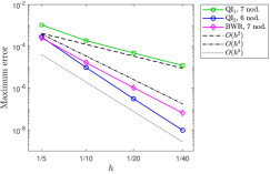
(a) Lower amount of nodes

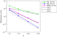
(b) Higher amount of nodes

Figure 1: Error convergence plots with respect to the mesh size $h$ for a type of integral $I_{B_{i}}[g]$ in Section 4.2.1.

4.2.2 Regular and singular integrals $I_{w_{i}^{s}}$

In the second example we measure the accuracy of the integrals with a term $K_{2}(s,t)=\log|s-t|$. The integrals are regular and singular integrals $I_{w_{h,i}^{s}}$, with the factor $w_{h.i}^{s}:=K_{2}(s,\cdot)\,B_{i,d}^{(\mathbf{T}_{h})}(\cdot)$, that appear as the inner integrals in $A^{(2)}_{i,j}$. For the test case we consider $g(t)=\sqrt{1+4t^{2}}$. The quadratic B-splines $B_{i,d}^{(\boldsymbol{T}_{h})}$ are constructed on the interval $[-1,\,1]$ with uniform open knot vectors ${\bf T}_{h}$ for the following mesh sizes $h=1/5,1/10,1/20,1/40$. The parameter $s$ is restricted to a priori chosen discrete values. Specifically, $s\in\boldsymbol{T}_{h/2}$, i.e., $s$ takes the values of all knots in the knot vector ${\bf T}_{h}$ and all the knot midpoints.

For every mesh size $h$ we measure the maximum error

$$\max_{i,s}|I_{w_{h,i}^{s}}-\tilde{I}_{w_{h,i}^{s}}|,$$

where the computed value of the integral obtained by a quadrature rule is denoted by $\tilde{I}_{w_{h,i}^{s}}$.

In the test we include also other suitable quadrature rules available in the literature. The hybrid Gauss-trapezoidal quadrature rules, sometimes called just Alpert rules (Alpert), is a class of quadratures for regular and singular functions, that comprise of special quadrature nodes and weights near the (regular or singular) edges of the integration domain [15]. The construction exploits a generalization of the Euler-Maclaurin summation formula. A common technique to accurately evaluate weakly singular integrals in BEM is the Telles transformation (Telles), which consists of applying a coordinate transformation to smooth out the singularity and then applying the standard Gaussian quadrature rule to evaluate the regularised integrals [17]. Finally, we also consider the singular weighted rule (SWR) [11]. Like $\text{QI}_{1}$ and $\text{QI}_{2}$, SWR is based on the precomputed modified moments but the construction of the weights requires to solve a global linear system.

By comparing the convergence error plots in Figure 2(a) and (b) for a fixed $h$ we can observe that all quadrature rules converge with the increased amount of quadrature nodes. Convergence with respect to $h$ reveals the convergence orders $O(h^{2})$ and $O(h^{5}|\log h|)$ for $\text{QI}_{1}$ and $\text{QI}_{2}$ scheme, respectively. The procedure $\text{QI}_{2}$ outperforms all other quadratures, and it is the only scheme with the optimal convergence order.

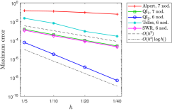
(a) Lower amount of nodes

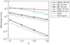
(b) Higher amount of nodes

Figure 2: Error convergence plots with respect to the mesh size $h$ for the regular and singular inner integrals $I_{w_{i}^{s}}$ in Section 4.2.2 for various quadrature rules available in literature.

4.2.3 Outer integrals in matrix $A^{(2)}$

In the last test we focus on regular integrals of the type

$$A_{h,i,j}^{(2)}:=-\frac{1}{2\pi}\int_{D_{i}}B_{i,d}^{(\mathbf{T}_{h})}(s)\,I_{w_{h,i}^{s}}\,ds$$ (29)

that appear as the outer integrals in (14) for $J\equiv 1$. The latter choice allows us to exactly evaluate the term $I_{w_{h,i}^{s}}$ in (29) by computing the corresponding modified moments (21). Therefore, the error of the numerical integration to compute $A_{h,i,j}^{(2)}$ is contributed solely by the quadrature to compute the outer integral (29). On interval $[-1,\,1]$ we construct uniform meshes with $h=2/5,1/5,1/10,1/20$.

In this test we include also the previously introduced B-spline weighted quadrature rule (BWR).

For each mesh size $h$ we measure the maximum error of integrals (29) for every $i$ and $j$,

$$\max_{i,j}\left|A^{(2)}_{h,i,j}-\tilde{A}^{(2)}_{h,i,j}\right|,$$

where $\tilde{A}^{(2)}_{h}(i,j)$ is the computed integral $A^{(2)}_{h}(i,j)$ with a quadrature rule. Surprisingly, the suboptimal convergence rate is obtained for all the quadratures, even though the function $I_{w_{h,i}^{s}}$ is well-defined and smooth. From Figure 3 we can observe the convergence order that is slightly higher than $O(h^{2})$. Again, the accuracy of the integral approximations is improved, when the amount of quadrature nodes is increased. This can be observed by comparing the plot Figure 3(a) for the lower and Figure 3(b) for the higher amount of nodes for a fixed $h$.

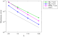
(a) Lower amount of nodes

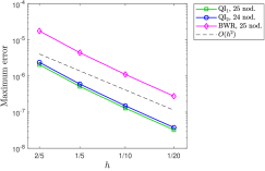
(b) Higher amount of nodes

Figure 3: Error convergence plots with respect to the mesh size $h$ for the outer integrals in $A^{(2)}$, defined in Section 4.2.3.

To clarify the suboptimal convergence in the test, we plot the function $I_{w_{h,i}^{s}}$ as a function of $s$ in Figure 4 for different fixed $h$ and $i$. For every mesh we plot the function only for the corresponding most central spline element, namely $i=4,7,12,22$. As we can see from the plot, the function $I_{w_{h,i}^{s}}$ is a smooth function of $s$ but the highest curvature actually increases with smaller $h$ (depicted as dots in the figure).

Figure 4: Function $I_{w_{h,i}^{s}}$ for different $h$ and $i$, from the test in Section 4.2.3.

Since the derivatives of $I_{w_{h,i}^{s}}$ are not bounded when $h\to 0$, the considered quadrature schemes cannot efficiently approximate this type of integrals with a fixed amount of nodes.

5 Numerical simulation with (Galerkin) BEM

In this section we test the boundary element model to numerically solve three Laplace boundary value problems. For all the examples we evaluate the governing integrals using the presented $\text{QI}_{1}$ and $\text{QI}_{2}$ quadrature schemes. In all cases we construct several successive approximate solutions of the problem by performing a dyadic $h$-refinement procedure on uniform meshes. We measure the relative error of an approximated solution against the exact one in $L^{2}$ norm with respect to degrees of freedom (DoF). The first numerical example is an exterior problem to an open curve, modelled by the indirect formulation. In the next two examples we employ the direct formulation to model interior problems to closed curves.

5.1 Exterior Dirichlet problem to arc of parabola

In this test we focus on the exterior problem described in [11], using the BIE (2.3). The Dirichlet BVP is defined in the exterior to an arc of parabola $\Gamma\in{\mathop{{\rm I}\kern-1.99997pt{\rm R}}\nolimits}^{2}$, parametrized by a quadratic B-spline curve ($d=2$). The transformation map ${{\bf F}}(s)=(s,1-s^{2})$, $s\in[-1,1]$, is described in terms of B-spline basis with the following knot vector $\bf T$ and set of control points $D$,

$${\bf T}=(-1,-1,-1,1,1,1),\qquad D=\begin{bmatrix}-1&&0&&1\\ 0&&2&&0\end{bmatrix}.$$

The Dirichlet datum $u_{D}$ and the exact solution $\phi$ are

$$(u_{D}\circ{{\bf F}})(s)$$

$$=\frac{-(7-9s+4s^{3})\log(2+2s+s^{2})-(7+9s-4s^{3})\log(2-2s+s^{2})}{12\pi}+\frac{14+24s^{2}}{9\pi}$$

$$+\frac{-(7+3s+4s^{3})\log(1+s)-(7-3s-4s^{3})\log(1-s)-(-1+12s^{2})\arctan\left(\frac{2}{s^{2}}\right)}{6\pi},$$

$$(\phi\circ{{\bf F}})(s)=\sqrt{1+4s^{2}}.$$

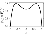
(a) Dirichlet datum

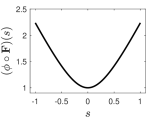
(b) Exact solution

(c) Initial mesh

Figure 5: Parabola test in Section 5.1: The Dirichlet datum, the exact solution and the initial mesh.

The Dirichlet datum, the exact solution, and the initial mesh in the physical domain are depicted in Figure 5. Observe that, although the function $u_{D}\circ{\bf F}$ is well defined for $s\in(-1,1)$, its derivative is not bounded when $s\to\pm 1$ and can represent an additional limitation for the quadrature $\text{QI}_{1}$, which needs also the derivative information on the integrand.

The convergence orders of the approximate solutions are shown in Table 1 for the quasi–interpolant degree $p=2$. Procedure $\text{QI}_{1}$ has a reduced accuracy near both the edges of the parametric domain. To get the optimal convergence $O(h^{d+1})$ for all refinement steps, a relative high amount of quadrature nodes is needed, $n+1=49$. On the other hand, it is sufficient to use a small amount of quadrature nodes, $n+1=7$, for the procedure $\text{QI}_{2}$.

Table 1: Parabola test in Section 5.1: Errors and convergence orders of the approximated solutions using quadrature rules $\text{QI}_{1}$ and $\text{QI}_{2}$, and $p=2$.

	$\text{QI}_{1}$, $n+1=49$		$\text{QI}_{2}$, $n+1=7$
DoF	error	conv.	error	conv.
12	$1.55\cdot 10^{-4}$		$1.57\cdot 10^{-4}$
22	$1.66\cdot 10^{-5}$	3.69	$1.66\cdot 10^{-5}$	3.70
42	$2.00\cdot 10^{-6}$	3.27	$2.00\cdot 10^{-6}$	3.27
82	$2.44\cdot 10^{-7}$	3.14	$2.45\cdot 10^{-7}$	3.14
162	$3.06\cdot 10^{-8}$	3.05	$3.05\cdot 10^{-8}$	3.06
322	$3.95\cdot 10^{-9}$	2.98	$3.22\cdot 10^{-9}$	3.27

5.2 Interior Dirichlet problem to a circle

To verify the correctness of the model using the direct formulation (2.3), we consider a simple boundary value problem. The geometry $\Gamma$ is a circle with radius $1/2$, described by the map ${{\bf F}}(s)=1/2\,[\cos(\pi s),\,\sin(\pi s)]^{T}$ for $s\in[-1,1]$. We note that due to the properties of the logarithmic kernel the choice of the radius can greatly influence the condition number of the matrix $A$ and hence the overall results. As analysed and explained in [26], if the radius is equal to one the problem becomes ill-posed and the computed system matrix becomes highly ill-conditioned.

For the chosen exact solution $u=x$, the Dirichlet datum is $(u_{D}\circ{{\bf F}})(s)=1/2\cos(\pi s)$ and the exact flux is $(\phi\circ{{\bf F}})(s)=\cos(\pi s)$.

The approximate solution is sought in the space of cubic B-splines ($d=3$) with the equally spaced extended knot vector

$${\bf T}=(-2,\,-5/3,\,-4/3,\,\dots,\,4/3,\,5/3,\,2).$$

The exact solution and the initial mesh in the physical domain are depicted in Figure 6.

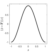
(a) Exact solution

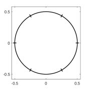
(b) Initial mesh

Figure 6: Circle test in Section 5.2: The exact solution and the initial mesh.

In Table 2 we report errors and convergence rates for the approximate solutions for different amount of DoF. For $\text{QI}_{1}$ we need to take $p=d$ to satisfy the projector property (see Section 3.2), whereas for $\text{QI}_{2}$ it is enough to consider $p=2$. To obtain the optimal convergence order $4$ for all the refinement steps, we need to considerably increase the amount of quadrature nodes for quadrature $\text{QI}_{1}$ ($n+1=25$), while for $\text{QI}_{2}$ we can maintain a small amount of nodes ($n+1=5$).

Table 2: Circle test in Section 5.2: Errors and convergence orders of the approximated solutions using quadrature rules $\text{QI}_{1}$ for $p=3$ and $\text{QI}_{2}$ for $p=2$.

	$\text{QI}_{1}$, $n+1=25$		$\text{QI}_{2}$, $n+1=5$
DoF	error	conv.	error	conv.
6	$1.66\cdot 10^{-3}$		$1.73\cdot 10^{-3}$
12	$7.69\cdot 10^{-5}$	4.43	$8.26\cdot 10^{-5}$	4.39
24	$4.40\cdot 10^{-6}$	4.13	$4.67\cdot 10^{-6}$	4.14
48	$2.69\cdot 10^{-7}$	4.03	$2.78\cdot 10^{-7}$	4.07
96	$1.67\cdot 10^{-8}$	4.01	$1.70\cdot 10^{-8}$	4.03
192	$1.05\cdot 10^{-9}$	4.00	$1.05\cdot 10^{-9}$	4.02

5.3 Interior Dirichlet problem to S curve

In the last numerical example we consider a problem with a more involved geometry, a domain described by the closed S curve [11]. The curve is parametrized by cubic B-splines with the knot vector $\bf T$ and set of control points $D$,

$${\bf T} =(-9/6,\,-9/6,\,-9/6,\,-9/6,\,-8/6,\,-7/6,\,\dots,\,7/6,\,8/6,\,9/6,\,9/6,\,9/6,\,9/6),$$

$$D =\setcounter{MaxMatrixCols}{15}\begin{bmatrix}3&4&7&6.5&5.2&7.3&7.1&6.4&3.8&4.7&5.3&3&3&4&7\\ 3.2&2.2&4&5.8&7.3&8.5&9.2&9.5&8&6.6&5&4.3&3.2&2.2&4\end{bmatrix}.$$

The boundary Dirichlet datum is set to $u_{D}(x,y)=x+y$ and the exact solution reads $(\phi\circ{{\bf F}})(s)=(-F^{\prime}_{1}(s)+F^{\prime}_{2}(s))/\|{{\bf F}}^{\prime}(s)\|_{2}$. The exact solution and the initial mesh in the physical domain are depicted in Figure 7.

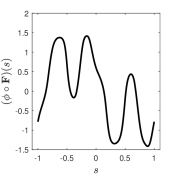
(a) Exact solution

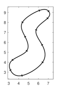
(b) Initial mesh

Figure 7: S curve test in Section 5.3: The exact solution and the initial mesh.

In Table 3 (top) we report errors for the approximate solutions when $C^{2}$ cubic test functions ($d=3$) are used. Again, for $\text{QI}_{1}$ we set $p=3$ and $p=2$ for $\text{QI}_{2}$. Since the exact solution $\phi\circ{\bf F}$ is only $C^{1}$ regular, a reduced order of convergence for the approximate solution is expected. This is confirmed by our experiments where the average convergence order is around 2.5.

In Table 3 (bottom) we can observe an improved convergence order 3 if we employ $C^{1}$ quadratic test functions ($d=2$) since the test functions have the same regularity as the exact solution. Here $p=2$ for both the quadrature rules. Of course, in this setting the space to describe the geometry is not a subspace of the test space $S_{h}$.

To conclude this test, we consider also a case with cubic test functions ($d=3$) that are $C^{1}$ smooth on the initial mesh by using double knots. More precisely, the discretization space $S_{h}$ consists of basis functions that are $C^{1}$ regular at the initial knots, and $C^{2}$ continuous at the inserted knots, obtained by dyadic refinements. In this setting, the space to describe the geometry is a subspace of $S_{h}$ for every step size $h$. Note that, in this case for the periodic compatibility $\rho=d-m+1=2$ (see Section 2.2). The results for the errors and convergence orders are reported in Table 4 for $\text{QI}_{2}$ with $p=2$, $n+1=7$ and $n+1=13$. A higher amount of quadrature nodes is necessary to recover the optimal order 4 for the approximate solution. The quadrature scheme $\text{QI}_{1}$ is not considered in this test since every basis function $B_{i,d}^{(\boldsymbol{T})}\in S_{h}$ should belong to the quasi–interpolation space $\hat{S}_{\boldsymbol{\tau}}$ and the involved quasi–interpolation operator cannot handle multiple knots.

Table 3: S curve test in Section 5.3: Error and convergence orders for $C^{2}$ cubic (top) and $C^{1}$ quadratic (bottom) test functions.

	$\text{QI}_{1}$, $n+1=25$		$\text{QI}_{2}$, $n+1=7$
DoF	error	conv.	error	conv.
12	$1.20\cdot 10^{-1}$		$1.30\cdot 10^{-1}$
24	$3.26\cdot 10^{-2}$	1.88	$3.50\cdot 10^{-2}$	1.89
48	$4.46\cdot 10^{-3}$	2.87	$4.52\cdot 10^{-3}$	2.95
96	$6.30\cdot 10^{-4}$	2.82	$6.46\cdot 10^{-4}$	2.81
192	$1.05\cdot 10^{-4}$	2.59	$1.07\cdot 10^{-4}$	2.59
384	$1.82\cdot 10^{-5}$	2.52	$1.86\cdot 10^{-5}$	2.53

	$\text{QI}_{1}$, $n+1=13$		$\text{QI}_{2}$, $n+1=7$
DoF	error	conv.	error	conv.
12	$1.24\cdot 10^{-1}$		$1.26\cdot 10^{-1}$
24	$2.76\cdot 10^{-2}$	2.17	$2.79\cdot 10^{-2}$	2.17
48	$2.96\cdot 10^{-3}$	3.22	$2.98\cdot 10^{-3}$	3.23
96	$2.55\cdot 10^{-4}$	3.53	$2.58\cdot 10^{-4}$	3.53
192	$2.50\cdot 10^{-5}$	3.35	$2.53\cdot 10^{-5}$	3.35
384	$2.92\cdot 10^{-6}$	3.10	$2.84\cdot 10^{-6}$	3.16

Table 4: S curve test in Section 5.3: Error and convergence orders for cubic test functions with $C^{1}$ smoothness at the initial knots, and $C^{2}$ regularity at the inserted knots.

	$\text{QI}_{2}$, $n+1=7$		$\text{QI}_{2}$, $n+1=13$
DoF	error	conv.	error	conv.
24	$2.92\cdot 10^{-2}$		$2.65\cdot 10^{-2}$
36	$7.12\cdot 10^{-3}$	3.48	$6.67\cdot 10^{-3}$	3.40
60	$7.28\cdot 10^{-4}$	4.46	$6.69\cdot 10^{-4}$	4.50
108	$4.64\cdot 10^{-5}$	4.68	$3.08\cdot 10^{-5}$	5.23
204	$5.51\cdot 10^{-6}$	3.35	$1.73\cdot 10^{-6}$	4.53
396	$8.99\cdot 10^{-7}$	2.73	$1.31\cdot 10^{-7}$	3.88

6 Conclusion

A study of the two recently introduced spline quasi–interpolation quadrature schemes is performed in the context of boundary integral equations in Galerkin IgA-BEM. A comparison of the accuracy of the schemes was already done in [1], when considering singular integrals. The analysis with respect to the amount of employed quadrature nodes revealed the optimal order of convergence for both approaches.

In the present paper, numerical tests show a notable difference between the two schemes. For a fixed amount of quadrature nodes the accuracy of the considered integrals is examined, when performing $h$-refinement of the approximation space. The observed rate of convergence is optimal only for the second scheme. In the numerical simulations for the 2D Laplace problems, the optimal order of convergence of the approximate solution is achieved with a small number of quadrature nodes, when the second procedure is employed. Regarding the first procedure, the amount of nodes should be increased to recover the optimal order for all the $h$-refinement steps.

In the future work we would like to investigate quadrature schemes for integrals of higher order singularities for more complex differential problems. A valuable contribution would be to derive stable formulae for the modified moments to simplify the construction of the proposed methods.

References

References

- [1] F. Calabrò, A. Falini, M. Sampoli, A. Sestini, Efficient quadrature rules based in spline quasi-interpolation for application to IgA-BEMs, J. Comput. Appl. Math. 338 (2018) 153–167.
- [2] M. Costabel, Principles of boundary element methods, Techn. Hochsch., Fachbereich Mathematik, 1986.
- [3] S. Sauter, C. Schwab, Boundary element methods, Vol. 39 of Springer Series in Computational Mathematics, Springer-Verlag, Berlin, Heidelberg, 2011.
- [4] R. Simpson, S. Bordas, J. Trevelyan, T. Rabczuk, A two-dimensional Isogeometric Boundary Element Method for elastostatic analysis, Comput. Methods Appl. Mech. Engrg. 209–212 (2012) 87–100.
- [5] X. Peng, E. Atroshchenko, P. Kerfriden, S. Bordas, Isogeometric boundary element methods for three dimensional static fracture and fatigue crack growth, Comput. Methods Appl. Mech. Engrg. 316 (2017) 151–185.
- [6] M. Taus, G. Rodin, T. Hughes, Isogeometric analysis of boundary integral equations: High-order collocation methods for the singular and hyper-singular equations, Math. Models and Methods in Appl. Sci. 26 (8) (2016) 1447–1480.
- [7] L. Heltai, M. Arroyo, A. DeSimone, Nonsingular isogeometric boundary element method for Stokes flows in 3D, Comput. Methods Appl. Mech. Engrg. 268 (2014) 514–539.
- [8] A. Aimi, M. Diligenti, M. L. Sampoli, A. Sestini, Isogeometric Analysis and Symmetric Galerkin BEM: a 2D numerical study, Appl. Math. Comp. 272 (2016) 173–186.
- [9] A. Aimi, M. Diligenti, M. L. Sampoli, A. Sestini, Non-polynomial spline alternatives in Isogeometric Symmetric Galerkin BEM, Appl. Numer. Math 116 (2017) 10–23.
- [10] B. H. Nguyen, H. D. Tran, C. Anitescu, X. Zhuang, T. Rabczuk, An isogeometric symmetric galerkin boundary element method for two–dimensional crack problems, Comput. Methods Appl. Mech. Engrg. 306 (2016) 252–275.
- [11] A. Aimi, F. Calabrò, M. Diligenti, M. L. Sampoli, G. Sangalli, A. Sestini, Efficient assembly based on B-spline tailored quadrature rules for the IgA-SGBEM, Comput. Methods Appl. Mech. Engrg. 331 (2018) 327–342.
- [12] F. Mazzia, A. Sestini, The BS class of Hermite spline quasi-interpolants on nonuniform knot distributions, BIT 49 (3) (2009) 611–628.
- [13] F. Mazzia, A. Sestini, Quadrature formulas descending from BS Hermite spline quasi-interpolation, J. Comput. Appl. Math. 236 (2012) 4105–4118.
- [14] A. Falini, C. Giannelli, T. Kanduč, M. L. Sampoli, A. Sestini, An adaptive IGA-BEM with hierarchical B-splines based on quasi-interpolation quadrature schemes, arXiv:1807.03563v2 (2018, submitted) .
- [15] B. Alpert, Hybrid Gauss-trapezoidal quadrature rules, SIAM J. Sci. Comput. 20 (1999) 1551–1584.
- [16] F. Calabrò, G. Sangalli, M. Tani, Fast formation of isogeometric Galerkin matrices by weighted quadrature, Comput. Methods Appl. Mech. Engrg. 316 (2017) 606–622.
- [17] J. Telles, A self-adaptive co-ordinate transformation for efficient numerical evaluation of general boundary element integrals, International journal for numerical methods in engineering 24 (5) (1987) 959–973.
- [18] C. de Boor, A practical guide to splines, revised Edition, Vol. 27 of Applied Mathematical Sciences, Springer-Verlag, New York, 2001.
- [19] G. Farin, D. Hansford, The essentials of CAGD, A. K. Peters/CRC Press, New York, USA, 2000.
- [20] W. Wendland, On some mathematical aspects of boundary element methods for elliptic problems, in: J. Whiteman (Ed.), The Mathematics of Finite Elements and Applications, Vol. 5 of Mafelap 1984, Academic Press Ltd., London, 1985, pp. 193–227.
- [21] K. Mørken, Some identities for products and degree raising of splines, Contr. Approx. 7 (1991) 195–208.
-
[22]
P. Sablonnière, A
quadrature formula associated with a univariate spline quasi interpolant,
BIT 47 (4) (2007) 825–837.
doi:10.1007/s10543-007-0146-8.
URL http://dx.doi.org/10.1007/s10543-007-0146-8 - [23] P. Sablonnière, D. Sbibih, M. Taharichi, Error estimate and extrapolation of a quadrature formula derived from a quartic spline quasi–interpolant, BIT 50 (4) (2010) 843–862.
- [24] A. Aimi, M. Diligenti, Numerical integration in 3D galerkin BEM solution of HBIEs, Comput. Mech. 28 (2002) 233–249.
- [25] T. Lyche, K. Mørken, Spline methods draft, University of Oslo 226 (2008) 12.
- [26] W. Dijkstra, R. Mattheij, A relation between the logarithmic capacity and the condition number of the BEM-matrices, Comm. Numer. Methods Engrg. 23 (7) (2007) 665–680.