Curvature correction to the field emission current

Abstract

The curvature of field emitter tips leads to an altered tunneling potential that assumes significance when the radius of curvature is small. We provide here an analytical curvature-corrected formula for the field emission current from smooth vertically aligned emitter tips and test its applicability across a range of apex radius, $R_{a}$, and local electric field, $E_{a}$. It is found to give excellent results for $R_{a}>10$nm with errors generally less than $10\%$. Surprisingly, for the uncorrected potential, we find the errors to be high even at $R_{a}=100$ nm ($>35\%$  at $E_{a}=3$ V/nm) and conclude that curvature correction is essential for apex radius less than a micron.

I Introduction

With the increasing use of nanostructured materials such as carbon nanotubes, nanowires and nanocones teo ; parmee ; spindt91 ; lee2002 ; baylor in field emission cathodes, the need for an extension to the Fowler-Nordheim (FN) formalism FN ; Nordheim ; murphy ; forbes ; forbes_deane ; jensen_ency to deal with emission from nano-tipped emitters is recognized KX ; jensen_image ; fursey ; db_imag ; db_ext . For emitters with apex radius of curvature $R_{a}$ in the nanometer regime, there are competing influences that determine the net field emission current from an isolated emitter. While the local electric field on the emitter surface increases with $1/R_{a}$ due to increased field enhancement, the tunneling potential on the other hand becomes wider as corrections to the external and image potential start contributing. These factors influence the local current density on the emitter surface, but, for purposes of determining the net emission current, the decrease in net emission area with increasing curvature must also be factored in. This interplay has added complexity when a large area field emitter (LAFE) is studied db_rudra since shielding effects and the spatial density of emitters become important in determining the net emitted current.

At the zeroth level, curvature effects are incorporated in the planar FN formalism in terms of the apex field enhancement factor $\gamma_{a}$ such that the local field $E({\bf{r}})=\gamma({\bf{r}})E_{0}$ at a point ${\bf{r}}$ on the emitter surface. Here $E_{0}$ is the macroscopic or asymptotic field far away from the emitter tip. Thus, the current density is expressed as murphy ; forbes_deane

$$J({\bf{r}})=\frac{1}{t_{F}^{2}}\frac{A_{\small{\rm FN}}}{W}E^{2}({\bf{r}})e^{-{B}_{\small{\rm FN}}{\nu}_{F}W^{3/2}/E({\bf{r}})}.$$ (1)

In the above, the free electron model is assumed and barrier lowering due to the image potential is incorporated so that the net potential experienced by the electron (Schottky-Nordheim barrier Schottky ; Nordheim ) is

$$V(s)=\phi-eEs-\frac{e^{2}}{16\pi\epsilon_{0}s}$$ (2)

where $E$ is the local field on the surface of the emitter and $s$ measures the distance normal to the emitter surface. In Eq. 1 above, $A_{\small{\rm FN}}~{}\simeq~{}1.541434~{}{\rm\mu A~{}eV~{}V}^{-2}$ and $B_{\small{\rm FN}}~{}\simeq~{}6.830890~{}{\rm eV}^{-3/2}{\rm V~{}nm}^{-1}$ are the conventional FN constants, $\phi={\cal E}_{F}+W$ where $W$ is the work function and ${\cal E}_{F}$ the Fermi energy (both $W$ and ${\cal E}_{F}$ in eV), while forbes ; forbes_deane

$${\nu}_{F}({\bf r})={\nu}(f_{F}({\bf r})) \simeq 1-f_{F}+\frac{1}{6}f_{F}\ln f_{F}$$ (3)

$${t}_{F}({\bf r})={t}(f_{F}({\bf r})) \simeq 1+f_{F}/9-\frac{1}{18}f_{F}\ln f_{F}$$ (4)

are correction factors due to the image potential, with $f_{F}=f_{F}({\bf r})\simeq 1.439965E({\bf{r}})/W^{2}$.

Eq. 1 serves well to analyze experimental data under conditions compatible with the model assumptions as well for curved emitters with radius of curvature much larger than the tunneling distance lambda ; Mayer . When the emitter tip radius is small, the flat-emitter assumption breaks down. It is not very clear at what apex radius of curvature this occurs even though some studies suggest KX that this could be around $R_{a}=20$nm. Our investigations here reveal that curvature dependent corrections are essential for radius of curvature as large as $R_{a}=1~{}\mu$m when the net emission current is of interest and the acceptable error is $5\%$.

The first few curvature correction terms to the tunneling potential of Eq. 2 are now known for any point near the emitter apex KX ; fursey ; jensen_image ; db_imag ; db_ext . These can be incorporated to obtain a suitably corrected expression for the tunneling transmission coefficient and hence the current density. It is assumed here that the field lines can be considered linear in the tunneling region even for curved emitters and 1-dimensional semiclassics continues to hold. For very small apex radius of curvature ($R_{a}<5$ nm) however, the field lines are likely to be curved even in the tunneling region and the curvature corrections in the potential must be accompanied by a multi-dimensional tunneling treatment. There are other factors in a real system that are not accounted for in this simplified picture. For instance, field electron emission must be treated in conjunction with space-charge effects which can further distort tunneling paths. We shall ignore these complications and merely assume that the field lines are approximately linear and along the normal to the emitter surface in the tunneling regime.

In the following, we shall briefly review the corrections to the tunneling potential and deal with the corresponding corrections to the transmission coefficient, the current density and the net emitted current. This is followed by our numerical results for the hemi-ellipsoid where exact results are known. In the rest of this paper, we shall consider an axially symmetric vertically aligned emitter, parallel to the direction of the asymptotic electrostatic field, $E_{0}\hat{z}$.

II Curvature corrections

II.1 The tunneling potential

The tunneling potential in Eq. 2 is appropriate when the local radius of curvature is very large and curvature terms may be neglected. In general, both the image and external potential get modified. The image potential takes the form fursey ; jensen_image ; db_imag

$$-\frac{e^{2}}{16\pi\epsilon_{0}s}(1-\frac{s}{2R_{2}}+\ldots)\simeq-\frac{e^{2}}{16\pi\epsilon_{0}s(1+\frac{s}{2R_{2}})}$$ (5)

where $R_{2}$ is the second principle radius of curvature at a point on the emitter surface. Note that at the apex, $R_{2}=R_{a}$ where $R_{a}$ is the apex radius of curvature. Eq. 5 is essentially a local spherical approximation of the emitter surface and reflects the interaction between the electron at a distance $s$ from the emitter and its image charge having magnitude $eR_{2}/(R_{2}+s)$ placed at a distance $R_{2}^{2}/(R_{2}+s)$ from the centre of the sphere.

The external potential also changes in the tunneling region when the local radius of curvature is small. As mentioned earlier however, we shall continue to treat the field lines as approximately linear, even though we shall account for the change in magnitude of the field in the tunneling region. This can be partially justified by noting that at the apex of the vertically aligned emitter, the field line continues to be along the axis (hence linear) even as the magnitude of the field drops away from the apex. Since field emission in sharp emitters occurs predominantly near the apex (small effective emission area), the linearity approximation is justified.

The first order curvature corrected external potential at the apex KX for a general axially symmetric emitter is

$$V_{ext}^{(1)}(s)=-eEs\Big{[}1-\frac{s}{R_{a}}\Big{]}.$$ (6)

For points ${\bf r}$ close to the apex, analytical studies of the hemi-ellipsoid and hyperboloid emitters and numerical evidence from other geometries (such as the conical emitter) show that the external potential is well represented in the tunneling region by db_ext

$$V_{ext}(s)=-eEs\Big{[}1-\frac{s}{R_{2}}+\frac{4}{3}\big{(}\frac{s}{R_{2}}\big{)}^{2}\Big{]}$$ (7)

where $R_{2}$ is the second principle radius of curvature. The net curvature corrected tunneling potential is thus

$$V_{C}(s)=\phi-eEs\Big{[}1-\frac{s}{R_{2}}+\frac{4}{3}\big{(}\frac{s}{R_{2}}\big{)}^{2}\Big{]}-\frac{e^{2}}{16\pi\epsilon_{0}s(1+\frac{s}{2R_{2}})}.$$ (8)

It is implicit here that the potential depends on the position ${\bf r}=(\rho,z)$ on the axially symmetric emitter surface through the local field $E=E({\bf r})$ and the radius of curvature $R_{2}=R_{2}({\bf r})$. For vertically aligned emitters db_ultram

$$E({\bf r}) = E_{a}\cos\tilde{\theta},~{}~{}\text{where}$$ (9)

$$\cos\tilde{\theta} = \frac{z/h}{\sqrt{(\rho/R_{a})^{2}+(z/h)^{2}}}$$ (10)

where $E_{a}$ is the local field at the apex and

$$R_{2}=R_{a}\Big{[}1+\big{(}\frac{\rho}{R_{a}}\big{)}^{2}\Big{]}^{1/2}.$$ (11)

It is assumed that the tip is smooth and can be expressed locally as $z=h-\rho^{2}/(2R_{a})$. With these additional inputs, the net field emission current can in principle be calculated for highly curved emitter tips.

In the following, we shall use the form of the tunneling potential as given in Eq. 8. However, for the sake of comparison, we shall also use the first order correction and denote it by

$$V_{C}^{(1)}(s)=\phi-eEs\Big{[}1-\frac{s}{R_{2}}\Big{]}-\frac{e^{2}}{16\pi\epsilon_{0}s(1+\frac{s}{2R_{2}})}.$$ (12)

II.2 The curvature corrected current density

Assuming a free electron model, the current density is evaluated at zero temperature as

$$J=\frac{2me}{(2\pi)^{2}\hbar^{3}}\int_{0}^{{\cal E}_{F}}T({\cal E})({\cal E}_{F}-{\cal E})d{\cal E}$$ (13)

where $T({\cal E})$ is the transmission coefficient at electron energy ${\cal E}$ measured with respect to the bottom of the conduction band, $m$ is the mass of the electron, $e$ is the magnitude of the electron charge and ${\cal E}_{F}$ is the Fermi level. Eq. 1 follows (i) on using the WKB expression for transmission coefficient

$$T_{WKB}({\cal E})=\exp\Big{(}-\frac{2}{\hbar}\sqrt{2m}\int_{s_{1}}^{s_{2}}\sqrt{V(s)-{\cal E}}~{}ds\Big{)},$$ (14)

in Eq. 13 with $V(s)$ given by Eq. 2, (ii) approximating the integral above as

$$\int_{s_{1}}^{s_{2}}\sqrt{V(s)-{\cal E}}~{}ds\simeq\frac{2}{3}\frac{(\phi-{\cal E})^{3/2}}{eF}{\nu}(f)$$ (15)

with $f\simeq 1.439965E({\bf{r}})/(\phi-{\cal E})^{2}$ and finally (iii) Taylor expanding it about the Fermi energy in order to carry out the energy integration. In the above $s_{1},s_{2}$ are the roots of $V(s)-{\cal E}=0$.

For the curvature corrected tunneling potential $V_{C}(s)$, a similar procedure can be followed. Following Ref. [12], the curvature corrected current density for the potential $V_{C}$ can be expressed by replacing $\nu_{F}$ and $t_{F}$ respectively in Eq. 1 by $\tilde{\nu}_{F}$ and $\tilde{t}_{F}$ apex_same . The curvature corrected current density at any point around the apex is thus first_second_same

$$J_{C}({\bf{r}})=\frac{1}{({\tilde{t}}_{F})^{2}}\frac{A_{\small{\rm FN}}}{W}E^{2}({\bf{r}})e^{-{B}_{\small{\rm FN}}{\tilde{\nu}}_{F}W^{3/2}/E({\bf{r}})}.$$ (16)

where

$${\tilde{\nu}}_{F}({\bf r}) = {\nu}_{F}({\bf r})+\frac{W}{E({\bf r})R_{2}({\bf r})}w_{F}({\bf r})~{}~{}$$ (17)

$${\tilde{t}}_{F}({\bf r}) = {t}_{F}({\bf r})+\frac{W}{E({\bf r})R_{2}({\bf r})}\psi_{F}({\bf r})~{}~{}$$ (18)

$$f_{F} = f_{F}({\bf r})\simeq 1.439965\frac{E({\bf{r}})}{W^{2}}$$ (19)

and

$$w_{F}({\bf r})=w(f_{F}({\bf r})) = \frac{4}{5}-\frac{7}{40}f_{F}-\frac{1}{200}f_{F}\ln(f_{F})$$ (20)

$$\psi_{F}({\bf r})=\psi(f_{F}({\bf r})) = \frac{4}{3}-\frac{1}{500}f_{F}-\frac{1}{30}f_{F}\ln(f_{F}).$$ (21)

The adequateness of Eq. 16 as a curvature-corrected current density is best tested on evaluation of the net emitted current. We shall therefore postpone a discussion on its merits till the next section.

II.3 The curvature corrected emission current

The current from an emitter tip can be evaluated by integrating the current density over the emitter surface:

$$I=\int J({\bf{r}})2\pi\rho\sqrt{1+(dz/d\rho)^{2}}d\rho$$ (22)

where ${\bf{r}}=(\rho,z)$. For smooth axially symmetric vertically aligned emitters, $z=h-\rho^{2}/(2R_{a})$ near the tip. Thus,

$$I=\int J({\rho})2\pi\rho\sqrt{1+(\rho/R_{a})^{2}}d\rho$$ (23)

or, alternately, in terms of the normalized angledb_distrib $\tilde{\theta}$ ,

$$I\simeq 2\pi R_{a}^{2}\int J(\tilde{\theta})~{}\frac{\sin\tilde{\theta}}{\cos^{4}\tilde{\theta}}d\tilde{\theta}.$$ (24)

Numerical evaluation of the current $I$ can be performed by typically integrating Eq. 23 from 0 to $R_{a}$ using appropriate forms of the current density.

We shall first dwell on the necessity and domain of applicability of the corrections to the tunneling potential. In order to establish this numerically, consider a hemi-ellipsoid on a grounded conducting plane in the presence of an asymptotic field $E_{0}\hat{z}$. The exact analytical form of the potential for this system is well known. The various forms of the tunneling potential that we shall compare with are (i) zeroth order as in Eq. 2 (ii) first order as in Eq. 12 and (iii) second order as given in Eq. 8. The errors in net emission current for these potentials can be computed relative to the analytical tunneling potential along (a) the normal to the surface (b) along the field line approx_fieldline . As remarked earlier, the normal to the surface and the field line approximately coincide in the tunneling region if the curvature is not too sharp.

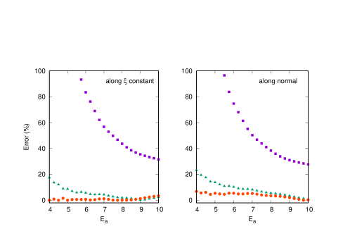
Figure 1: The error in net emission current using the $0^{th}~{}\text{(squares)}$, $1^{st}~{}\text{(triangle)}$ and $2^{nd}~{}\text{(circle)}$ order tunneling potentials relative to the analytical tunneling potential computed along field lines ($\xi=\text{constant}$,left) and along normal to the surface (right). The apex radius of the hemiellipsoid $R_{a}=13$ nm.

Fig. 1 shows the error in net emission current using the zeroth order (Eq. 2, filled squares), first order (Eq. 12, filled triangle) and second order (Eq. 8,filled circle)) tunneling potentials. The errors are computed relative to the current found using the analytical potential (a) along field lines ($\xi=\text{constant}$ where ($\eta,\xi,\varphi$) are prolate spheroidal co-ordinates approx_fieldline ; smythe ) and (b) along normal. In all cases, the transfer matrix method DBVishal is adopted for the transmission coefficients. Note that at $R_{a}=13$ nm, the error is large for the first order tunneling potential at lower local apex field strengths. For smaller apex radius, the errors for both the zeroth and first order tunneling potential are much larger.

Figure 2: As in Fig. 1 for apex radius of curvature $R_{a}=50$ nm.

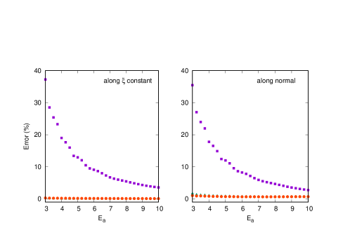
Figure 3: As in Fig. 1 for $R_{a}=100$ nm.

At $R_{a}=50$ nm, it is still worthwhile to use the second order correction to the tunneling potential for lower apex fields as seen in Fig. 2. The error for the zeroth order decreases but remains large. At $R_{a}=100$ nm (Fig. 3), the first order and second order corrections are hard to distinguish even at lower field strengths and while the error for the zeroth order potential decreases further, the curvature-corrected potential must still be used especially at lower fields. At $R_{a}=500$nm, the error in using the zeroth order potential falls to $7\%$ at $E_{a}=3$ V/nm while at $R_{a}=1~{}\mu$ m and $E_{a}=3$ V/nm, the error is 5.3%. Thus, it is profitable to use the second order corrected potential for $R_{a}<1~{}\mu$m, especially at lower field strengths.

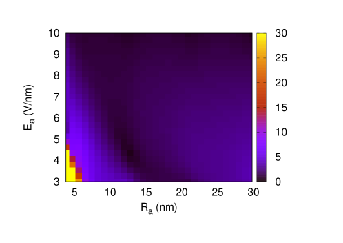
Figure 4: The relative % error in the net emission current calculated using Eq. 16 for ellipsoidal emitters with varying apex radius of curvature $R_{a}$ and local apex field $E_{a}$. The error is relative to the option (c) using Eq. 25.

Having established that the second order tunneling potential (Eq. 8) is essential for curved emitters when $R_{a}<1~{}\mu$m, we next turn our attention to the efficacy of the curvature corrected current density of Eq. 16. The total emitted current can be calculated using Eq. 23 along with Eq. 16 and the value obtained can be compared using one of the following alternative (and more exact) methods of obtaining the current density: (a) transfer matrix or equivalent “exact” evaluation of the transmission coefficient DBVishal at all energies and exact energy integration (b) an exact WKB evaluation of the transmission coefficient (Eq. 14 with $V$ replaced by $V_{C}$) at all energies and an exact energy integration (c) Taylor expansion (upto the linear term) of Eq. 14 around the Fermi energy and exact evaluation of all the integrals. Clearly, the current evaluated using Eq. 16 is expected to be closest to option (c) above. The current density in option (c) can be expressed as

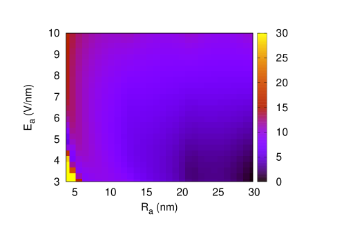
Figure 5: The relative % error in the net emission current calculated using Eq. 16 relative to the current determined using option (b) where the exact WKB transmission coefficient is used together with exact energy integration.

$$\begin{split}J=&\frac{2me}{(2\pi)^{2}\hbar^{3}}\int_{0}^{{\cal E}_{F}}({\cal E}_{F}-{\cal E})\exp\Big{[}-g\int_{s_{1}}^{s_{2}}\sqrt{V_{C}(s)-E_{F}}\Big{]}\times\\ &\exp\Big{[}(E-E_{F})\frac{g}{2}\int_{s_{1}}^{s_{2}}\frac{1}{\sqrt{V_{C}(s)-E_{F}}}~{}ds\Big{]}d{\cal E}\end{split}$$ (25)

with the integrals evaluated numerically. Eq. 25 together with Eq. 23 gives the total emitted current. Here $s_{1}$ and $s_{2}$ are zeroes of $V_{C}(s)-E_{F}=0$.

Fig. 4 shows the error in net emission current evaluated using $J_{C}$ (Eq. 16) relative to that obtained using Eq. 25. Clearly, the relative error is small for $R_{a}>7$nm at all field strengths considered while for smaller apex radius, error is larger when $R_{a}E_{a}$ is small as expected from the nature of the correction.

We next compute the error in net emission current evaluated using $J_{C}$ relative to option (b) above where the exact WKB transmission coefficient is used together with the exact energy integration. Note that the exact WKB transmission coefficient is determined by evaluating the Gamow exponent

$$G=g\int_{s_{1}}^{s_{2}}\Big{(}V_{C}(s)-{\cal E}\Big{)}^{1/2}$$ (26)

exactly. Here $g=2\sqrt{2m}/\hbar\simeq 10.246~{}(\text{eV})^{-1/2}(\text{nm})^{-1}$. The integral is performed numerically in order to determine $G$ and hence the transmission coefficient. The relative error is shown in Fig. 5. The error is somewhat larger compared to the previous case since the energy integration is exact in option (b) while Eq. 16 uses a Taylor expansion in energy. For $R_{a}>10$nm however, the error is reasonably small. Note also that option (b) is close to the exact transfer matrix result calculated using option (a) with errors within $1\%$ in the region of interest.

II.4 An approximate analytical expression for net current

For an approximate analytical expression, Eq. 24 can be used together with the curvature corrected current density $J_{C}$ expressed in terms of $\tilde{\theta}$ as db_distrib

$$J(\tilde{\theta})=\frac{1}{\tilde{{t}}_{F}(\tilde{\theta})^{2}}\frac{A_{\small{\rm FN}}}{W}E_{a}^{2}\cos^{2}\tilde{\theta}~{}e^{-B_{\small{\rm FN}}\tilde{{\nu}}_{F}(\tilde{\theta})W^{3/2}/(E_{a}\cos\tilde{\theta})}.$$ (27)

Eq. 27 follows on using Eq. 9 in Eq. 16. Thus,

$$I\simeq{\cal C}\int_{0}^{\pi/3}\frac{\sin\tilde{\theta}}{\cos^{2}\tilde{\theta}}\frac{1}{{\tilde{t}}_{F}^{2}(\tilde{\theta})}e^{-{\cal B}{\tilde{\nu}}_{F}(\tilde{\theta})/\cos\tilde{\theta}}d\tilde{\theta}$$ (28)

where

$${\cal C} = 2\pi R_{a}^{2}\frac{A_{\small{\rm FN}}}{W}E_{a}^{2}~{}~{}~{}\text{and}$$ (29)

$${\cal B} = \frac{B_{\small{\rm FN}}W^{3/2}}{E_{a}}$$ (30)

With the substitution $1/\cos\tilde{\theta}=1+x$, Eq. 28 reduces to db_distrib

$$I\simeq{\cal C}\int_{0}^{1}\frac{1}{{{\tilde{t}}_{F}^{2}(x)}}e^{-{\cal B}{\tilde{\nu}}_{F}(x)(1+x)}dx.$$ (31)

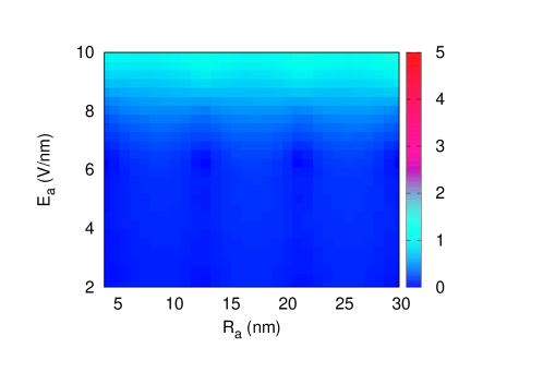
Figure 6: The relative % error in the net emission current calculated using Eqns. 38 and 40, relative to emission current calculated using Eq. 16.

Since the dominant contribution comes from the neighbourhood of $x=0$, a Taylor expansion of ${\tilde{\nu}}_{F}(x)(1+x)$ and $1/{\tilde{t}}_{F}^{2}(x)$ at $x=0$ can be used. Keeping only the linear termdb_distrib ,

$${\tilde{\nu}}_{F}(x)(1+x) = \tilde{D}_{0}+\tilde{D}_{1}x+\mathcal{O}(x^{2})$$ (32)

$$\frac{1}{{\tilde{t}}_{F}^{2}(x)} = \tilde{F}_{0}+\tilde{F}_{1}x+\mathcal{O}(x^{2})$$ (33)

where

$$\tilde{D}_{0} = {\nu}_{F}(0)+{\cal X}_{F}w_{F}(0)$$ (34)

$$\tilde{D}_{1} = \big{(}1-\frac{f_{0}}{6}\big{)}+{\cal X}_{F}\big{(}\frac{4}{5}+\frac{f_{0}}{200}\big{)}$$ (35)

$$\tilde{F}_{0} = \frac{1}{\big{[}t_{F}(0)+{\cal X}_{F}\psi_{F}(0)\big{]}^{2}}$$ (36)

$$\tilde{F}_{1} = \frac{f_{0}-f_{0}\ln f_{0}+{\cal X}_{F}\frac{3}{5}\big{(}\frac{53}{50}f_{0}+f_{0}\ln f_{0}\Big{)}}{9\big{[}t_{F}(0)+{\cal X}_{F}\psi_{F}(0)\Big{]}^{3}}$$ (37)

with ${\cal X}_{F}=W/(E_{a}R_{a})$ and $f_{0}=1.439965E_{a}/W^{2}$. Note that the quantities, ${\nu}_{F}(0)$, $w_{F}(0)$, $t_{F}(0)$ and $\psi_{F}(0)$ are calculated at the apex. Thus,

$$I\simeq 2\pi R_{a}^{2}J_{C}(0)\tilde{{\cal G}}$$ (38)

where

$$\tilde{{\cal G}}=\frac{1}{{\cal B}\tilde{D}_{1}}+\frac{\tilde{F}_{1}}{\tilde{F}_{0}}\frac{1}{({\cal B}\tilde{D}_{1})^{2}}$$ (39)

determines the effective emission area at the apex. In effect, the first term

$$\tilde{{\cal G}}\simeq\frac{1}{{\cal B}\tilde{D}_{1}}$$ (40)

gives excellent results relative to the current derived using Eq. 16. A comparison of the errors in current determined using Eqns. 40 and Eq. 38 relative to the current evaluated using Eq. 16 is shown in Fig. 6. Clearly, the approximate analytical formula does not introduce significant errors as compared to a direct use of Eq. 16 for finding the current.

Figure 7: Error in the emission current computed using Eqns. 40 and Eq. 38 relative to the exact potential along the normal for various apex radius $R_{a}$. The local apex field $E_{a}$ is measured in V/nm.

When compared to the current computed using the exact analytical potential along the normal, the error is found to be generally below $10\%$ over a wide range of local apex field strengths when $R_{a}>10$nm as seen in Fig. 7. The increase in error away from $E_{a}\simeq 5$V/nm is likely due to the Taylor expansion in energy as discussed earlier.

Figure 8: Error in the emission current computed using the second order tunneling potential of Eq. 8 relative to the exact potential along field lines.

Finally, we revisit the domain of applicability of the second order potential $V_{C}(s)$. A comparison of the currents obtained by transfer matrix method using the exact potential along field lines ($\xi=\text{constant}$) and the second order tunneling potential of Eq. 8 is shown as an error map in Fig. 8. The errors increase sharply for $R_{a}$ less than $10$ nm especially for the smaller apex fields and is therefore not shown. The errors for $R_{a}>10$ nm are generally below $5\%$ thus validating the use of the second order curvature corrected potential.

III Conclusions

We have investigated the curvature corrected field emission current density and the net emission current using a form of the tunneling potential that has been found to hold in analytically solvable emitter models and numerically verified for other emitter shapes. It was found that curvature correction is essential for apex radius of curvature smaller than a micron with errors using the uncorrected potential as high as 37% at $R_{a}=100$ nm and around $5\%$ at $R_{a}=1~{}\mu$m at $E_{a}=3$ V/nm.

Using recent results, the curvature corrected current density at any point of the emitter surface was derived and subsequently used to calculate the net emission current. This was used as a basis for finding a simple analytical expression for the net emitted current from axially symmetric vertically aligned smooth (parabolic) emitter tips. It was found that the curvature corrected easy-to-use formula for emission current agreed to within 10% of the exact result for $R_{a}>10$nm and to within $5\%$ if the transfer matrix method is used with the curvature corrected potential.

IV Acknowledgement

The authors acknowledge several useful discussions with Dr. Raghwendra Kumar and Gaurav Singh.

 

V References

References

- (1) K. B. K. Teo, E. Minoux, L. Hudanski, F. Peauger, J. P. Schnell, L. Gangloff, P. Legagneux, D. Dieumegard, G. .A.J. Amaratunga and W. I. Milne, Nature 437, 968 (2005).
- (2) R. J. Parmee, C. M. Collins, W. I. Milne, and M. T. Cole, Nano Convergence 2, 1 (2015).
- (3) C. A. Spindt, C. E. Holland, A. Rosengreen and I. Brodie, IEEE Trans. on Electron Devices, 38, 2355 (1991).
- (4) C. J. Lee et al., Appl. Phys. Lett. 81, 3648 (2002).
- (5) L. R. Baylor, V. I. Merkulov, E. D. Ellis, M. A. Guillorn, D. H. Lowndes, A. V. Melechko, M. L. Simpson, J. H. Whealton, J. Appl. Phys., 91, 4602 (2002).
- (6) R. H. Fowler and L. Nordheim, Proc. R. Soc. A 119, 173 (1928).
- (7) L. Nordheim, Proc. R. Soc. A 121, 626 (1928).
- (8) E. L. Murphy and R. H. Good, Phys. Rev. 102, 1464 (1956).
- (9) R. G. Forbes, App. Phys. Lett. 89, 113122 (2006).
- (10) R. G. Forbes and J. H. B. Deane, Proc. Roy. Soc. A 463, 2907 (2007).
- (11) K. L. Jensen, Field emission - fundamental theory to usage, Wiley Encycl. Electr. Electron. Eng. (2014).
- (12) A. Kyritsakis and J. P. Xanthakis, Proc. R. Soc. London, A471, 20140811 (2015).
- (13) K. L. Jensen, D. A. Shiffler, J. R. Harris, I. M. Rittersdorf, and J. J. Pettilo, J. Vac. Sci. Technol., B 35, 02C101 (2017).
- (14) G. N. Fursey and D. V. Glazanov, J. Vac. Sci. Technol. B 16, 910 (1998).
- (15) D. Biswas and R. Rajasree, Phys. Plasmas, 24, 073107 (2017); 24, 079901 (2017).
- (16) D. Biswas, R. Rajasree and G. Singh, Phys. Plasmas 25, 013113 (2018).
- (17) D. Biswas and R. Rudra, Shielding effects in random large area field emitters, the field enhancement factor distribution and current calculation Phys. Plasmas (in press).
- (18) W. Schottky, Physik. Zeitschr. 15, 872 (1914).
- (19) Even in this regime, Eq. 1 does not acurately predict the current density for all local fields, work function or Fermi energy, even though, the semiclassical transmission coefficient on which it is based, is reasonably accurate. This is due to a Taylor approximation of the transmission coefficient around the Fermi energy while performing the integration over all electron energies. More accurate results can however be computed numerically or using the table of coefficients in Mayer Mayer to account for a factor to be used alongside Eq. 1.
- (20) A. Mayer, J. Vac. Sci. Tech. B, 29, 021803 (2011).
- (21) D. Biswas, G. Singh, S. G. Sarkar and R. Kumar, Ultramicroscopy 185, 1 (2018).
- (22) D. Biswas, Phys. Plasmas, 25, 043105 (2018).
- (23) This is identical to the corrected apex current density of Ref. [12] since at the apex.
- (24) Since this in a Taylor expansion in evaluated at , the coefficient of is identical for and .
- (25) Close to the vertically aligned hemi-ellipsoid surface, can be considered to be along the field line. Further away, the field lines deviate away from and asymtotically point in the vertical direction.
- (26) W. R. Smythe, Static and Dynamic Electricity, Taylor and Francis (1989).
- (27) D. Biswas and V. Kumar, Phys. Rev. E 90, 013301 (2014).