Search and Return Model for Stochastic Path Integrators

Abstract

We extend a recently introduced prototypical stochastic model describing uniformly the search and return of objects looking for new food sources around a given home. The model describes the kinematic motion of the object with constant speed in two dimensions. The angular dynamics is driven by noise and describes a “pursuit” and “escape” behavior of the heading and the position vectors. Pursuit behavior ensures the return to the home and the escaping between the two vectors realizes exploration of space in the vicinity of the given home. Noise is originated by environmental influences and during decision making of the object. We take symmetric $\alpha$-stable noise since such noise is observed in experiments. We now investigate for the simplest possible case, the consequences of limited knowledge of the position angle of the home. We find that both noise type and noise strength can significantly increase the probability of returning to the home. First, we review shortly main findings of the model presented in the former manuscript. These are the stationary distance distribution of the noise driven conservative dynamics and the observation of an optimal noise for finding new food sources. Afterwards, we generalize the model by adding a constant shift $\gamma$ within the interaction rule between the two vectors. The latter might be created by a permanent uncertainty of the correct home position. Non vanishing shifts transform the kinematics of the searcher to a dissipative dynamics. For the latter we discuss the novel deterministic properties and calculate the stationary spatial distribution around the home.

There exists search at global scales and local search centered around a given home position. In the latter case, the searcher does not only look for a new target but is also required to permanently return to the home position. Such behavior is typical for many insects and achieves technical importance for self-navigating robotic systems. We propose a stochastic nonlinear model for local search which does not distinguish between the two aims. The dynamics bases on an unique pursuit and escape behavior of the heading from the position vector realizing thereby optimal exploration of space and the return to the home. We discuss the mechanics of the searcher and inspect the role of noise. Such randomness is present in the decision making rule of selecting the new heading direction. We consider Levy noises with different degree of discontinuity and report about steady spatial densities for the searchers. Also we report about an optimal noise intensity that a searcher finds a target at nearby places where the spatial distribution of the searcher is maximal.

I Introduction

The usage of different kinds of noise in global search problems is very popular Bénichou et al. (2011). For non-local search applications of Lévy Flights and of various types $\alpha$-stable white noise have provenKlages (2017) to be very effective. However, applications of such kinds of noise in models of local search are very rare. Local search reduces the exploration of the neighborhood of a certain localization. The use of power law distributed step length to explore the neighborhood of a certain spot seems to be counterproductive.

Such local search is observed for objects which are able to keep track of distances and orientations as they move and use these informations to calculate their current position in relation to a fixed location. The latter can be a nest or a source of food and is called home Mittelstaedt and Mittelstaedt (1980). If the position of the home and the angle towards the home are known then the method is called path integration Mittelstaedt and Mittelstaedt (1980); Cheng (1995); Wang (2003); Klages (2017) and the specific exploration behavior might be based on some internal storage mechanism Seelig and Jayaraman (2015); Green et al. (2017) or external cues Zeil (2012) as for example special points of interest or pheromonic traces, etc.

In our model studied below we orientate on studies and experiments concerned with ants, bees and fliesWehner, Michel, and Antonsen (1996); el Jundi (2017); Kim and Dickinson (2017). For these animals such homing behavior is found. Especially, the various two dimensional spatial patterns which the local searchers draw during their motion have received a lot of interest Wehner and Srinivasan (1981); Wehner, Michel, and Antonsen (1996); Vickerstaff and Merkle (2012); Waldner (2018). A similar deterministic kernel of the heading dynamics as considered below was introduced earlier by Vickerstaff and Di Paolo Vickerstaff and Di Paolo (2005) based on Mittelstaedts’ investigations Mittelstaedt (1962). But their profound mathematical explanation based on principles of nonlinear and stochastic dynamics seems to be still a challenge.

In a broader sense, the better understanding of local search problems is of high technical interest. Nowadays a new age of spatial exploration Chien and Wagstaff (2017) has started, in which robots are reaching places that human beings have never approached, with explorer robots being projected for missions in ocean Hook et al. (2013); Girdhar et al. (2011); Leonard et al. (2007); Dubowsky et al. (2005), space Chien and Wagstaff (2017); Dubowsky et al. (2005), etc. Such applications as, for example, an autonomous spacecraft or search and rescue missions require autonomy since the vehicles must be able to make decisions and cannot be idle while waiting for directions.

Also homing behavior and local search in engineering applications are of relevance to autonomous navigation in systems of surveillance, data collection, exploration, monitoring, etc. Autonomous vehicles Leonard et al. (2007); Duarte et al. (2016) might move inside an area, around a chosen point, sometimes visit it and return to the local search using internal cues instead of external ones Nirmal and Lyons (2016); Möller et al. (2001).

In a recent manuscript we introduced a novel stochastic model for local searchNoetel et al. (2018). Here, we extend the investigations on this stochastic model, that considers an active particle with constant speed in two dimensions. The constant speed is common in a variety of models Mikhailov and Meinköhn (1997); Romanczuk et al. (2012) and also observed in experiments with insects Kim and Dickinson (2017).

Our model aims to mimic the motion of simple organisms, self-navigating automata or other moving objects which shall explore the surrounding space and return to its home. We implement the local search around the home via a coupling term between the heading angle of the particle and the angle formed by its current position and the home. The coupling is defined in an uniform way for the search epoch as well as for the return one. Hence we do not distinguish between the two aims.

We assume that the searcher possesses an internal storage mechanism. In a Cartesian frame of reference two angles are stored while in the reference frame of polar coordinates the spatial distance and the angle between the heading direction and the direction towards the home needs to be known. We point out, that in our model no knowledge of the distance towards the home is required in a Cartesian frame of reference. This is in contrast to similar path integrators Vickerstaff and Di Paolo (2005). However, in the reference frame of polar coordinates the particle would perform path integration. The resulting spatial motion allows the particle to explore the vicinity of the home in order to find new food sources and the searchers consecutively return to the home.

In section II, we briefly review the model. In sections II.1 and II.2 we report on central findings in Noetel et al. (2018). The presentation of the latter in the current manuscript is necessary for the understanding of the novel aspects considered below. This discussion concentrates on results with noise present.

In the next section III we extend our investigation and consider a situation with a limited knowledge of the position of the home. The escape-pursuit aligning mechanism between the two vectors is weakened by introducing a shift in the interacting rule. As a consequence the motion of the searcher starts to become dissipative and collapses to a limit cycle in the two dimensional space. We calculate the approximative spatial densities for large and small noise intensities. Finally, we summarize our findings in section IV.

Special attention is paid to the influence of the random decision process of the searcher. The noise therein originates from an uncertainty in the definition of heading direction for the active particle. This uncertainty is related to neural processing and decision making of the new direction. Reasons are in a vagueness about the exact position of the home or in a limited capability to choose an exact direction of motion due to external perturbations.

In many studies on stochastic nonlinear dynamics, Gaussian white noise is applied as source of dynamical randomness. However, we model the noise as symmetric $\alpha$-stable white noise source which also includes the case of a Gaussian noise with the particular choice $\alpha=2$. Inclusion of white Lévy noise in this local search problem was stimulated by findings in experiments with the fruit fly Drosophila Melanogaster Kim and Dickinson (2017). The authors of this study report on a Lévy-kind statistics in the angular dynamics during the local search of the fruit fly. Despite those randomness acting with heavy tails, the wrapping of the dynamic angles onto the interval $(-\pi,\pi]$ will allow asymptotically the establishment of a continuous steady state distribution of the searchers around the home. As will be elaborated below, the latter is centered around home without the introduced shift. Otherwise, searchers accumulate probability in a crater-like shape above the stochastic limit cycles if the shift hinders precise orientation.

II The Search and Return Model

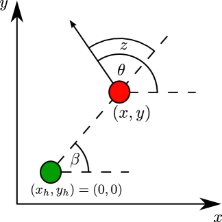
Figure 1: Schematic introduction of position and heading vector with angles $\beta(t)$ and $\theta(t)$. The difference between the two angles is assigned by $z(t)=\theta(t)-\beta(t)$. The searching object is colored red and moves in two dimensions with the Cartesian position $x(t)$ and $y(t)$. The home possesses color green and is situated for convenience at the origin. The distance of the searcher from the home is $r(t)=\sqrt{x(t)^{2}+y(t)^{2}}$.

We consider an active Brownian particle Romanczuk et al. (2012) whose position vector is given by $\vec{r}(t)=\{x(t),y(t)\}$. This position vector reads in polar coordinates $\vec{r}(t)=r(t)\{\cos(\beta(t)),\sin(\beta(t))\}$ with distance $r(t)$ and direction $\beta(t)$. We assume that the searcher moves with constant speed $v_{0}$

$$\dot{\vec{r}}=\vec{v}(t)=v_{0}\begin{pmatrix}\cos\theta(t)\\ \sin\theta(t)\end{pmatrix}\,,$$ (1)

$\dot{\vec{r}}$ denotes the temporal derivative of the position vector $\vec{r}$ and $\theta$ is the heading angle of the particle pointing along the velocity vector as is depicted in Figure 1.

Since the home is situated at the origin of the Cartesian reference frame, the position vector $\vec{r}$ points always out of the home towards the particle’s current position. The corresponding angle $\beta(t)\in[0,2\pi)$ is given by:

$$\beta(t)=\arctan{\frac{y(t)}{x(t)}},$$ (2)

as also sketched in Figure 1. When arriving the home $x(t_{a})=y(t_{a})=0$, both vectors are anti-parallel $\beta(t_{a}-0)=\theta(t_{a})+\pi$. Inertia would require that the object leaves the home with $\beta(t_{a}+0)=\theta$. Inspired by the behavior of the fruit flies, we discuss at the end of the search study in Sect.(II.2.2) a random reset of the heading in close proximity to the home.

The search and return dynamics is part of the evolution rule for the heading angle $\theta(t)\in[0,2\pi)$. We require that $\dot{\theta}$ evolves in time as

$$\dot{\theta}=\kappa\sin(\theta-\beta)+\frac{\sigma}{v_{0}}\xi(t).$$ (3)

The first item is the deterministic drift term of this equation. It might be motivated by a escape and pursuit behavior Romanczuk, Couzin, and Schimansky-Geier (2009) of the position and velocity vectors. For positive values of the parameter $\kappa$, if $\theta(t)\in\{\beta(t)-\pi/2,\beta+\pi/2\}$, the velocity vector is repelled from the position vector. It is the situation where the velocity vector also points out of home and the object still leaves the home. Thereby, a separation of the two vectors guarantees a larger exploration of the space in the vicinity of the home. Otherwise, if $\theta(t)\in\{-\beta(t)-\pi/2,-\beta+\pi/2\}$ the velocity vector is pointing oppositely to the position vector. In this situation the searcher is already on the way home. To find the position of the home an alignment, i.e. an attraction of the two vectors, is preferable as described by Eq.(3).

In the second term on the r.h.s. of Equation (3) $\xi(t)$ stands for a source of symmetric $\alpha$-stable white noise. The simulations were performed considering an Euler integration step for the deterministic drift and the noise is implemented following Weron and Weron (1995); Janicki and Weron (1994); Nolan (2018). For details see Appendix A. It serves as an uncertainty in the definition of the heading direction at time $t$. It might be caused by a limited knowledge of either the heading direction, itself, or of the angle between the current position of the particle and the home $\beta$. Generally, it stands for the decision making step of the searcher to choose a new direction. The noise strength is $\sigma$. In the case of $\alpha=2$, increments of the angle are uncorrelated in time and with Gaussian support.White noise with $\alpha<2$ in the angular dynamics yields a continuous description for a run and tumble like motion with fast tumbling epoch Nötel, Sokolov, and Schimansky-Geier (2017) as it was also found and reported in the experimental study Kim and Dickinson (2017).

Further on, we will cross to a dimensionless description. Let us assign the dimensionless time as $t^{\prime}=\kappa t$ and the dimensional position from the origin as $\vec{r^{\prime}}(t^{\prime})=\vec{r}(t^{\prime})/r_{c}$ with $r_{c}=v_{0}/\kappa$. Afterwards one gets for the new temporal variables $x^{\prime}(t^{\prime}),y^{\prime}(t^{\prime}),\theta^{\prime}(t^{\prime})$ the dimensionless deterministic dynamics. For simplicity, we reassign $t^{\prime}\rightarrow t,x^{\prime}(t^{\prime})\rightarrow x(t),y^{\prime}(t^{\prime})\rightarrow y(t),\theta^{\prime}(t^{\prime})\rightarrow\theta(t)$ and get

$$\frac{\rm d}{{\rm d}t}\,x=\cos(\theta)\,,$$ (4)

$$\frac{\rm d}{{\rm d}t}\,y=\sin(\theta)\,,$$ (5)

$$\frac{\rm d}{{\rm d}t}\,\theta=\sin(\theta-\beta)+\frac{\sigma^{\prime}}{v_{0}}\xi(t)\,,$$ (6)

with $\beta(t)=\arctan(y(t)/x(t))$. Notable, the deterministic dynamics depends only on the dimensionless initial coordinates. We get the dimensionless equations from the outgoing ones by selecting simply $\kappa=1$ and $v_{0}=1$. In contrast, the noise intensity has to be rescaled and reads $\sigma^{\prime}=\sigma/\kappa^{1/\alpha}$ and the $v_{0}$ remains in front of the noise source in the dimensionless frame. But likewise for the other values we omit the prime and replace $\sigma^{\prime}\rightarrow\sigma$. Later on in simulations, we take for simplicity values of $\kappa$ and $v_{0}$ always equal to unity. Another choice would imply a multiplicative rescaling of the noise intensity.

We underline that the proposed model is an uniform evolution law for both, search and return. Our model does not artificially distinguish between a search period and a return period as it is assumed for several observed food searchers such as ants Vickerstaff and Merkle (2012). There is no switcher between the two aims and both episodes of the evolution are described by a single function. It is also worth to mention that other functions similarly to the considered sine in (3) are able to exhibit similar effects as discussed, later on.

II.1 Deterministic Dynamics

Let us shortly remind deterministic properties of the considered model. With this purpose we put $\sigma=0$ in (3). After introducing the difference of the two angles $z(t)=\theta(t)-\beta(t)$ and crossing to polar coordinates with the distance $r(t)$ and the angle $\beta$ the deterministic dynamics reads

$$\frac{\rm d}{{\rm d}t}\,r=\cos(z)\,,$$ (7)

$$\frac{\rm d}{{\rm d}t}\,z=\left(1-\frac{1}{r}\right)\sin(z)\,,$$ (8)

$$\frac{\rm d}{{\rm d}t}\,\beta=\frac{1}{r}\sin(z)\,.$$ (9)

One immediately notices that the $\beta(t)$ evolution is determined by the dynamics in the $r,z$-plane. Finding $r(t),z(t)$ gives the $\beta$-evolution by integration of the last equation. Therefore, the deterministic case reduces to the motion in the $r,z$-plane. This yields except for $z=\pm\pi$ and $z=0$ bounded oscillatory solutions which remind of trajectories within the celestrial mechanics, but in the considered case with constant speed Noetel et al. (2018).

For $z=\pm\pi,0$ the value of $z$ (and $\beta$) does not change and the distance grows unlimited or vanishes, respectively. Approaching with $z=\pm\pi$ the value $r=0$, the trajectory jumps quickly to $z=0$ from which it grows unbounded $r(t)\to\infty$. In the stochastic case, these trajectories are without any relevance since the angular noise will change permanently the $z$-value and, hence, a constant value of $z$ will not hold. As consequence, these unbounded trajectories have zero measure in the stochastic frame.

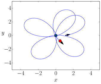
Figure 2: Left: Periodic deterministic trajectory in $x,y$ frame with anti-clockwise perihel precession during one rotation with $x_{0}=1,y_{0}=0,\theta_{0}=\pi/16$. Right: Trajectories in $(r,z)$ plane according to Equation (10) for initial conditions $r_{0}=1,z0\in,[-\pi/2,\pi/2]$ starting at the arrow-positions. Different colors stand for different values of $X$ resulting from different initial conditions $r_{0},z_{0}$. The green dot represents the home position.

All other deterministic motion is bounded. The dynamics in $r,z$ forms closed orbit around two centers at $r_{0}=1,z=\pm\pi/2$ with imaginary eigenvalues $\pm{\rm i}$. Every closed orbit possesses an integral of motion $X(r,z)=const$. To derive this the time is eliminated considering a parametric dependence of the two variables $z(r)$. In the equation for ${\rm d}r/{\rm d}z$ the variable can be separated and we obtain by quadrature Noetel et al. (2018)

$$X=\sin(z(r))\exp\left(-r\right)r=\sin(z_{0})\exp\left(-r_{0}\right)r_{0}={\rm const}.$$ (10)

The counterclockwise rotations and the anticlockwise ones, which result in dependence on the initial angle $z_{0}$, are presented in Fig.(2). Minimal and maximal distances of $r$ and $z$ can be easily derived. From these we can find the period of the motion $T(r_{0},z_{0})$ by integration of the first equation of (7) with inserted integral of motion $X$ instead of $z(t)$. It takes values closely to the eigenvalue near the centers and diverges for the larger orbits. Similarly one can integrate the $\beta$-dynamics and find a precession of the perihel in the $x,y$ space during one oscillation as shown in Fig.(2). Also the sign of the angular momentum $L=r^{2}\dot{\beta}=r\sin(z)$ does not change along one revolution since the $\sin$-function does not change the signNoetel et al. (2018).

II.2 The Stochastic Case

In case with noise we also cross to polar coordinates. The dynamics for the stochastic distance $r(t)$ and angle $\beta(t)$ does not change and is given by the Eqs.(7). In the dynamics for the stochastic angle difference $z(t)$ following Eq.(3) a stochastic source term with $\xi(t)$ appears. It becomes

$$\dot{z}=\left(1-\frac{1}{r}\right)\sin(z)+\frac{\sigma}{v_{0}}\,\xi(t)\,.$$ (11)

The noise acts on the angular dynamics, only. Particles are still moving with constant speed. The noise induces a population of all possible values of $z$ and smears the motion along all $X$ values in the $r,z$-plane. The unbounded motion becomes unlikely in the stochastic system and the searcher remains with high probability at finite distances from the home. Hence, the noise stabilizes the motion.

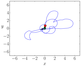
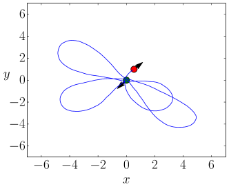
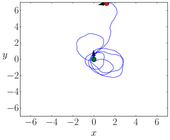
Figure 3: Sample stochastic trajectories with different noises in $(x,y)$ plane. Particle starts at $(0,0)$. Upper row: $\alpha=1$; Lower row: $\alpha=2$. Left: $\sigma^{\alpha}=0.01$; Right:$\sigma^{\alpha}=0.1$. Other parameter $v_{0}=1$.

In the stochastic case one has now two more parameters. One is $\alpha$ that characterizes the noise type. In addition we have $\sigma$, standing for the noise strength. We will report that the noise strength plays an important role for finding a new food source. Less important in our case is the noise type. The noise acts on the angle which is a $2\pi$-periodic variable. Hence the long tails of $\alpha$-stable noise are always wrapped on the bounded interval of possible $z$-values and do not influence significantly the stochastic evolution after relaxation to an uniform distribution in $z$.

Typical stochastic trajectories can be seen in Figure 3. The particles started at the home $(x,y)=(0,0)$ and moved for the time interval $\Delta t=50$. In the left column for small noise $\sigma^{\alpha}=0.01$ the deterministic drift mostly determines the motion of the particle, while on the right for larger noise $\sigma^{\alpha}=0.1$ the underlying deterministic part of the motion can practically no longer be recognized. The noise causes a diffusion in space of possible deterministic trajectories. As derived below in the next subsection (II.2.1) the stationary distance density is independent of the noise type $\alpha$ and the noise strength $\sigma$.

II.2.1 Stationary Density of Distances

An important measure for the behavior of the stochastic searcher is the stationary spatial distribution of the searchers. For this purpose, we introduce transition probability density function $P(r,z,t|r_{0},z_{0},t_{0})$ in dependence of the distance $r$ and angle difference $z$. This density obeys the corresponding Fokker-Planck equation (FPE) which, according to Ditlevsen (1999); Schertzer et al. (2001); Yanovsky et al. (2000) reads in the considered case

$$\frac{\partial}{\partial t}P=-\frac{\partial}{\partial r}\cos(z)P+\frac{\partial}{\partial z}\left(\frac{1}{r}-1\right)\sin(z)P+\left(\frac{\sigma}{v_{0}}\right)^{\alpha}\frac{\partial^{\alpha}}{\partial|z|^{\alpha}}P\,,$$ (12)

wherein

$$\frac{\partial^{\alpha}}{\partial|z|^{\alpha}}P(z)=-\frac{1}{2\pi}\int_{-\infty}^{\infty}\,{\rm{d}k}|k|^{\alpha}\,\exp\left(-ikz\right)\,P(k)$$ (13)

stands for the $\alpha$th symmetric Riesz-Weyl derivative, with $P(k)$ being the Fourier transform of $P(z)$ in the variable $z$. The drift term is due to the deterministic dynamics for the distance and the angle difference whereas the last term describes the influence of the $\alpha$-stable noise source. We remind that $r$ is non-negative and $z$ is $2\pi$-periodic.

In the asymptotic stationary limit $t\rightarrow\infty$ the initial conditions are forgotten and the density becomes stationary, i.e. $P(r,z,t\to\infty|r_{0},z_{0},t_{0})=P_{0}(r,z)$. Hence one might put $\partial P_{0}(r,z,t)/\partial t=0$. Further on , we separate

$$P_{0}(r,z)=P_{0}(r|z)P_{0}(z).$$ (14)

The noise distributes the probability homogeneously in $z$ since no angular direction is distinguished. Therefore, $P_{0}(z)=1/2\pi$. The fractional derivative for the wrapped constant angular pdf vanishes due to the symmetry of the noise. There is no effective force repelling the noisy $z$-shifts and also the asymptotic spatial distribution does not depend on $z$. For the latter radial pdf the equation remains to be solved:

$$0=\left[-\frac{\partial}{\partial r}+\frac{1}{r}-1\right]\cos(z)P_{0}(r)\,.$$ (15)

Therein the noise dependent item is absent. Dropping the $cos$-function we find the stationary radial pdf as Noetel et al. (2018)

$$P_{0}(r,z)=\frac{1}{2\pi}r\exp\left(-r\right).$$ (16)

The marginal distribution of distances follows immediately

$$P_{0}(r)=r\exp\left(-r\right).$$ (17)

It is shown in Fig.(4) and compared with numeric simulations for different noise types. Remarkably, the spatial density of the searcher is a Rayleigh distribution which is independent of the noise. It is independent with respect to the noise type expressed by $\alpha$ as well as to the noise intensity $\sigma$. It contains the characteristic dimensionless length $r=1$ which is the length with maximal probability. The mean distance is given by $<r>=2$ and the spatial coefficient of variation $CV_{r}=\sqrt{0.5}$ characterizing the spatial uncertainty of the random search. The typical shape is presented in Fig.(4)

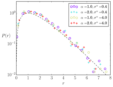
Figure 4: The stationary marginal radial pdf $P_{0}(r)$ from Eq.(17) (black dashed line). Symbols from simulations of the stochastic dynamics with different types and strength of the noise.

The stationary spatial density is also independent of $\beta$. Hence, in the Cartesian frame the pdf reads:

$$P_{0}(x,y)=\frac{1}{2\pi}\exp\left(-\sqrt{x^{2}+y^{2}}\right)$$ (18)

This pdf is maximal at the home.

Further on, we solved for arbitrary $\alpha\in(0,2]$ and $\sigma\neq 0$ the FPE (12) ,with the Ansatz $P=\exp(\lambda t)e(r,z)$, for the time dependent eigenfunction

$$e_{1}(r,z)=\sin(z)r^{2}\exp\left(-2r\right)\,,$$ (19)

with the eigenvalue $-1/\tau$. The fractional derivative governing the angle $z$ in (12) becomes when applied to the sine function, the sine function itself, with a minus sign in front of it. For details see appendix B.

As seen $\tau$ which is as defined as

$$\tau=\left(\frac{v_{0}}{\sigma}\right)^{\alpha}$$ (20)

obtains the meaning of a relaxation time of the angle difference in the stochastic case. After $t\gg\tau$ the spatial distribution becomes independent of any initial orientation $z_{0}$.

II.2.2 Optimal Noise for Search of a New Food Source

In this subsection we report on the influence of the noise to discover a new food source Noetel et al. (2018). We fixed the speed value $v_{0}=1$ in the stochastic source term of Eq.(11). Then the noise strength and its type are the tunable parameters in our stochastic model. To quantify the stochastic search for the target we obtained numerically mean times after that the searcher finds a food spot for the first time. We placed a target at $(x_{t},y_{t})=(1,0)$. We chose this distance $d=1$ from the home as at this distance the stationary spatial density becomes maximal for all noise types and strength.

With a given noise type and at each value of the noise strength we made $50000$ runs. The search started in the vicinity from home with radius $r_{0}$ of the home with random orientations. As the model is supposed to describe the search of living organisms, we assume the searcher has a sensing radius $r_{{\rm sens}}$. We do not consider a spatial extension of the target, as this can be put into the sensing radius. We determined the random search times needed to sense the target.

We consider the sensing radius to be small against the length scale $r_{c}$ of the system, then we chose for the simulations a value $r_{{\rm sens}}=0.1$. During its stochastic oscillatory search, the trajectory generally missed the target and returned several times to the home, passing the latter one to start the next round. After it found the target, we resetted the particle to the initial position and restarted for the next determination of the search time.

Figure 5 presents the mean first hitting time $<t>$ for a given food spot in dependence of the inverse relaxation time $1/\tau$. With the selected speed value, the latter is identical to the scaled noise intensity $\sigma^{\alpha}$.

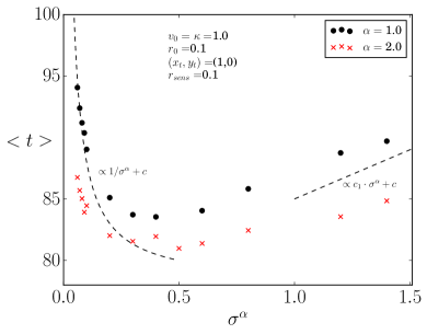
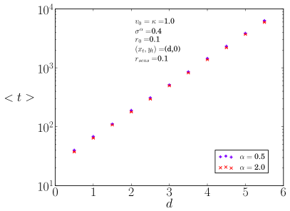
Figure 5: Left: Mean hitting time $<t>$ during search of a new spot at a given position $(x_{t}=1,y_{t}=0)$ found numerically in dependence of the noise intensity. Right: Mean time $<t>$ for a fixed noise intensity in dependence of the distances $d$, with $(x_{t}=d,y_{t}=0)$.

First of all, the mean first hitting times are always larger than the relaxation time $\tau$ as given by Eq.( 20). However, as presented in Fig.(5) an optimal noise strength can be seen where the mean search time becomes minimal Noetel et al. (2018). This optimal time does depend on the relaxation time $\tau$ or, respectively, on the scaled noise intensity $\sigma^{\alpha}$. Without noise, i.e. $\sigma=0$, some of the deterministic trajectories will never hit, or take extremely long. For example, some existing unbounded trajectories expanding radially away from the home and those which do not hit the target during the first expansion will do it never. Hence the mean hitting time diverges in the noise-less case.

Afterwards with low noise, the mean hitting times starts to decay nearly as $\propto C+1/\sigma^{\alpha}$ until reaching the minimum. Later on, for larger noise the hitting times scale with the noise intensity, i.e.$\propto\sigma^{\alpha}$. We also found that for larger distances to the target, the optimal noise shifts to smaller values (not shown here).

This non-monotonous dependence results from two counteracting effects induced by the noise. By means of the first one, trajectories will distribute over all possible orbits with different values of $X$. The characteristic time scale for this process is the angular relaxation time which scales as $\tau\propto 1/\sigma^{\alpha}$. This first effect determines the decay of $<t>$ at lower noise intensities.

The second effect created by the noise starts to act at larger values of the noise intensity. For these noise values, the deterministic dynamics becomes negligible. With large noise slow diffusive search becomes dominant. But as well known the corresponding diffusion coefficient of free active particles scales inversely with the noise. It decays asMilster et al. (2017) $D_{\rm eff}\propto 1/\sigma^{\alpha}.$ In consequence, the spatial relaxation needs longer for higher noise. The time reaching in average a certain distance $d$ in two dimensions by diffusion can be defined following

$$t_{\rm diff}=\frac{<d^{2}>}{4D_{\rm eff}}\propto\sigma^{\alpha}\,.$$ (21)

On the right of Fig. 5 we present the average search time for a fixed value of $\sigma^{\alpha}=0.4$ and different distances $d$ of the target. We find that the average search time grows exponentially with the distance.

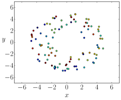
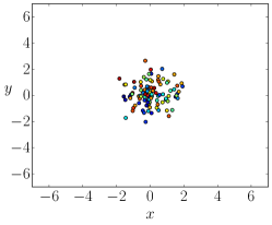
Figure 6: Spatial distribution of ensembles of $100$ searchers after simulation time $t=5$ for small $\sigma^{2}=0.01$, optimal $\sigma^{2}=0.4$ and large $\sigma^{2}=4$ Gaussian noise. Different colors of the particles correspond to different heading directions.

The different temporal behavior of the random search is illustrated in Fig.(6) where ensembles of $100$ stochastic searchers are presented for small, optimal and large noise after a given time $t$. Initial conditions for all pictures are equivalent, meaning the particles are started at a distance $r_{0}=0.1$ from the home and the angles $\beta$ and $\theta$ are uniformly distributed. In the left picture with small noise, the angular symmetry is given due to the random initial angles. But the single searcher follows still the deterministic dynamics along the orbit corresponding to the particular initial state since $t_{s}<\tau$. Hence, particular searchers move along the rigid deterministic paths. Such dynamics along an orbit might take the particle rather far away from the home. The searcher will be able in average to find localized targets after the slow perihel precession has slipped on most directions. In contrast, in the graph to the right the searchers do not extend far away in space due to limited diffusive motion. The motion of a single searcher is undirected. Its probability has already populated uniformly in all possible directions. The situation of the middle graph shows the desired situation. The probability density for the heading direction of a single searcher is already uniform. Searcher are fast transported in radial direction by the underlying deterministic dynamics and noise has spread the probability of singular searchers uniformly over all orbits. This circumstance guarantees a successful finding of the target.

Gaussian white noise always performed slightly better in the numerical simulations. When changing $\alpha$ to lower values we observed a small increase of the mean time $<t>$.

In Figures (7) and (8) results of a new situation are presented. There it was assumed that the searcher stays between two sequential excursions a negligible period at the home. The latter will not be counted but it shall be necessary that the searcher forgets the incoming direction of the last search. Thus, it starts after arrival the next search along an arbitrary direction which was randomly selected. We believe that such restart from home is closer for possible applications of food search.

Fig. (7) shows again typical trajectories with a random reset at the home. Fig. (8) presents the mean hitting times of a possible target at distances $d=0.5$ and $d=1$. At the distance $d=1$ the marginal radial pdf is extremal for all noise types and values of the noise strength. We find a general reduction of the mean search time due to the additional random effect.

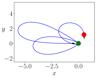
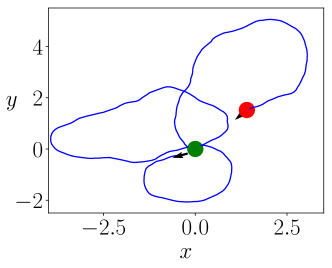
Figure 7: Sample stochastic paths with a random reset at home between two searching excursions. Left side is the deterministic noise free case. Right graph with optimal noise $\sigma^{\alpha}=0.4$.

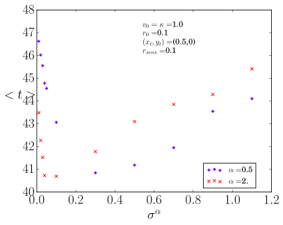
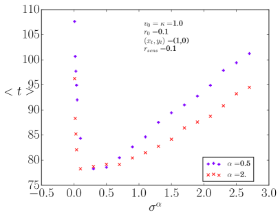
Figure 8: Mean hitting time $<t>$ during search of a new spot at two given positions with random reset at home. Left:$(x_{t}=0.5,y_{t}=0$);Right:$(x_{t}=1,y_{t}=0)$. The random reset of the searcher at a distance $r_{sens}=0.1$ from the home reduces the mean hitting times.

III Searchers With Limited Knowledge Of The Position Angle

The position angle $\beta$ influences the future heading direction as given by equation (3). In this section we investigate the consequences of a limited knowledge of the position angle. A limited knowledge means that the angle is not exactly known. To model this failure we introduce a constant offset $\gamma\in(-\pi/2,\pi/2)$ in the interaction rule of the heading and position vectors. That way we investigate in a simple way how the behavior of the searcher changes, if the understanding of the position angle is wrong. We will find, that even the slightest offset drastically changes the behavior of the particle, leading to the emergence of a limit cycle. The noise type as well as the noise strength however influence the pdf for being at the home and therefore for returning to it.

The time evolution of the heading direction $\theta$ becomes:

$$\dot{x}=v_{0}\cos(\theta)$$

$$\dot{y}=v_{0}\sin(\theta)$$

$$\dot{\theta}=\kappa\sin(\theta-\beta+\gamma)+\frac{\sigma}{v_{0}}\xi(t)\,.$$ (22)

Like in the original model, we consider the coupling strength $\kappa>0$ towards the home as constant. For $\gamma=0$ this model converges with the original model.

Following Sect. II, we introduce dimensionless variables and change to polar coordinates. The time evolution of the position angle $\beta(t)$ remains unchanged as formulated in Eq.(7). For the distance $r(t)$ and the angle difference $z(t)=\theta(t)-\beta(t)$, we get

$$\dot{r}=\cos(z)$$

$$\dot{z}=\left(\cos(\gamma)-\frac{1}{r}\right)\sin(z)+\sin(\gamma)\cos(z)+\frac{\sigma}{v_{0}}\xi(t)$$ (23)

with $\xi(t)$ being $\alpha$ stable white noise. We consider again the wrapped angle $z\in(-\pi,\pi]$.

III.1 The Deterministic Case

Equation (23) shows that an uncertainty of the position angle $\beta$ causes a change in the coupling strength towards the home expressed through the $\cos(\gamma)$ term and also causes an additional drift. Notably, for $|\gamma|=\pi/2$ the coupling towards the home vanishes and for $|\gamma|>\pi/2$ the coupling becomes repulsive. We restrict our discussion to $|\gamma|<\pi/2$.

Unlike before, the deterministic reduced $(r,z)$ dynamics (7) $(\sigma=0)$ is now dissipative. In addition to the repelling zero-distance if $r(t)\rightarrow 0$, it has now one stable and one unstable fixed points at

$$r_{*}=\frac{1}{\cos(\gamma)}\,$$ (24)

and

$$z_{\pm}=\pm\frac{\pi}{2}\,.$$ (25)

Surprisingly, the steady $z_{\pm}$-values do not depend on $\gamma$. The heading vector is always perpendicular to the position vector. In contrast, the stationary distance from the home of the fixed points increases with growing absolute value of $\gamma$ and reaches infinity if $|\gamma|\rightarrow\pi/2$. The key reason for the transition from the previous centers ($\gamma=0$) to a dissipative dynamics with stable and unstable fixed points is the emergence of the term with $\cos(z)$ on the r.h.s. of equation (23). It is proportional to the radial velocity $\dot{r}$ and vanishes for $\gamma=0$. This term causes that small deviations in the vicinity of $(r_{*},z_{\pm})$ either grow, or vanish. It means, that eigenvalues of the fixpoints for $\gamma\neq 0$ obtain a real part that is either negative, or positive.

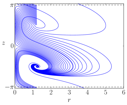
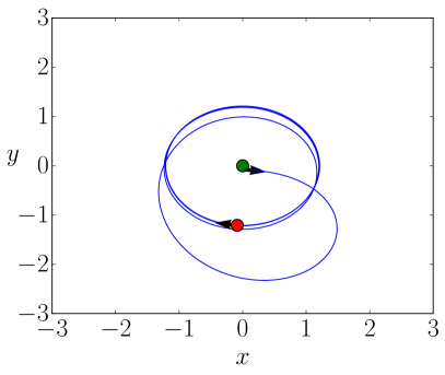
Figure 9: Left: Deterministic flow diagram of the dissipative wrapped dynamics in $r,z$ space with $\gamma=0.6$. Fix points are located at $r_{*}$ from Eq.(24) and $z=\pm\pi/2$. Initial conditions $r_{0}=r_{*}$ and $z_{0}\in[\pi/2,\pi]$. The focus in the lower half plane is stable whereas the upper one is unstable. Right: Deterministic motion in the $x,y$ plane. Approaching the stable fixed point, the searcher performs clockwise limit cycle oscillations in the $x,y$-space with heading vector perpendicularly to the position vector.

In order to discuss the stability of the fixed points, we expand Eq. (23) around the fixpoints $\{r_{*},z_{\pm}\}$ with small $\delta_{r}=r-r_{*}$ and small $\delta_{z_{\pm}}=z-z_{\pm}$ up to first order of $\delta_{r}$ and $\delta_{z_{\pm}}$. The radial velocity becomes

$$\dot{\delta}_{r}=\mp\delta_{z_{\pm}}$$ (26)

and for the angle follows

$$\dot{\delta}_{z_{\pm}}=\pm\cos^{2}(\gamma)\delta_{r}\mp\sin(\gamma)\delta_{z_{\pm}}\,\,.$$ (27)

Taking another time derivative of the second equation leads to

$$0=\ddot{\delta}_{z_{\pm}}\pm\sin(\gamma)\dot{\delta}_{z_{\pm}}+\cos^{2}(\gamma)\delta_{z_{\pm}}\,\,$$ (28)

the damped harmonic oscillator. The eigenvalues become, respectively, $\lambda_{\pm}=\mp\sin(\gamma)/2\pm\sqrt{5\sin^{2}(\gamma)/4-1}$, meaning that for $\gamma\in(0,\pi/2)$ the fixed point $(r_{*},z_{+})$ is stable and $(r_{*},z_{-})$ is unstable and vice versa for $\gamma\in(-\pi/2,0)$. It shall be also mentioned that values $\gamma\rightarrow\pi/2$ make the eigenvalues real and the foci becomes nodes.

The second term on the r.h.s. of (28) is responsible for damping. This term is a consequence of introducing $\gamma$. For $\gamma=0$ the eigenvalues have no longer a real part, the second term on the r.h.s. vanishes, so $(r_{*},z_{\pm})$ become centers.

Figure 9 shows trajectories for different initial conditions in the $(r,z)$ plane for $\gamma=0.6$. All trajectories converge to a single point $(r_{*},z_{-})$, except the one started at the unstable fixed point $(r_{*},z_{+})$.

Correspondingly sample trajectories in the $(x,y)$-plane converge to a circular oscillation with amplitude $r_{*}$ around the home in a clockwise fashion. The angular velocity follows from the $\beta$ dynamics $\dot{\beta}_{*}=-1/r_{*}=-\cos(\gamma)$. With positive $\gamma$ the $z_{+}$ becomes the stable fixpoint and the motion becomes anti clockwise around the home.

III.2 Small Noise Strength: Steady State - Gaussian White Noise

Having briefly discussed the deterministic motion, we will now consider the noise in the heading dynamics. Typical stochastic trajectories are presented in Fig. (10) for small noise intensity $\sigma^{\alpha}=0.01$ and two values of $\alpha$. The left graph shows the searcher driven by white Cauchy noise with $\alpha=1$. In the situation presented at the right we took Gaussian white noise with $\alpha=2$. One immediately observes, that the motion is more narrow around the stable circular orbit in case of Lévy noise than in the Gaussian case. Otherwise, in the Gaussian case the motion is not interrupted by stronger deviations as the appear in the first case due to the discontinuous character of the Lévy noise.

Next in subsection (III.2.1), we will consider the application of Gaussian white noise in the heading-dynamics. The other remaining parts (III.2.2) and (III.2.3) will deal with situations that small and large $\alpha$-stable noise is applied. The distinction is originated by different approximations made for the aim to obtain expressions for the stationary spatial densities of the searchers.

III.2.1 Small Noise Strength: Steady State - Gaussian White Noise

As the investigation of the deterministic case has shown, the searchers move independently of initial conditions eventually on a circle of radius $r_{*}$ around the home in Cartesian coordinates. With noise added the distribution in the $x,y$ plane possesses circular symmetry. Hence, the marginal distribution of the distances is sufficient in order to characterize the asymptotic behavior of the searcher. Unfortunately, we have been unable to derive a general solution and will look for approximations, further on. Here, we consider the linear equations (26) and (27). We have to note, that the variables therein $\delta_{r}$ and $\delta_{z}$ have lost the wrapped character. Both run between $-\infty$ and $\infty$ and have lost the meaning of a positive distance and a $2\pi$ periodic angle. It implies that we have to restrict the noise strength $\sigma$ to small values in the linear approximation. With small noise one avoids deviations where the character of a distance or periodicity becomes important.

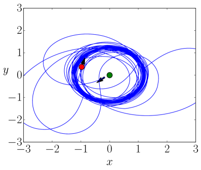
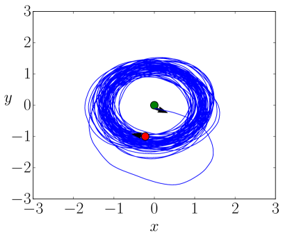
Figure 10: Stochastic trajectories of the searcher with shift $\gamma=-0.6$ in the interaction law starting at the home. Elapsed time during search: $t=500$. Left: $\alpha=1$, Right: $\alpha=2$. Whereas the fluctuations around the limit cycle at the left are more narrow, the jumps in case of $\alpha=1$ excite larger deviations. Other parameters: $v_{0}=1$, $\sigma^{\alpha}=0.01$

Consider $\gamma$ to be positive. The stable fixed point is located in the upper $r,z$- halfplane. We formulate the stochastic dynamics $(\delta_{r},\delta_{z})$ around $(r_{*},\pi/2)$ omitting the $\pm$ in the subscript of $\delta_{z}$. The corresponding FPE becomes

$$\frac{\partial}{\partial t}P(\delta_{r},\delta_{z},t)=\delta_{z}\frac{\partial}{\partial\delta_{r}}P-\frac{\partial}{\partial\delta_{z}}\left(\cos^{2}(\gamma)\delta_{r}P-\sin(\gamma)\delta_{z}P\right)+\left(\frac{\sigma}{v_{0}}\right)^{2}\frac{\partial^{2}}{\partial(\delta_{z})^{2}}P\,.$$ (29)

We will look for its stationary solutions $P(\delta r,\delta z,t\rightarrow\infty)\rightarrow P_{0}(\delta r,\delta z)$ for $\gamma\in(0,\pi/2)$ and equate the l.h.s. to zero. This problem of a noise driven harmonic oscillator was already solved by Ornstein and Uhlenbeck Uhlenbeck and Ornstein (1930), the steady state pdf is given by

$$P_{0}(\delta_{r},\delta_{z})=\frac{v_{0}^{2}\cos(\gamma)\,\sin(\gamma)}{2\pi\sigma^{2}}\exp\left(-\frac{v_{0}^{2}\sin(\gamma)\delta^{2}_{z}}{2\sigma^{2}}\right)\exp\left(-\frac{v_{0}^{2}\cos^{2}(\gamma)\sin(\gamma)\delta^{2}_{r}}{2\sigma^{2}}\right)\,.$$ (30)

As explained above, the variables $\delta_{z}$ and $\delta_{r}$ are here considered to be not wrapped.

Reintroducing the position $r$ and the angle results in

$$P_{0}(r,z)=\frac{v_{0}^{2}\cos(\gamma)\,\sin(\gamma)}{2\pi\sigma^{2}}\exp\left(-\frac{v_{0}^{2}\sin(\gamma)\left(z-\frac{\pi}{2}\right)^{2}}{2\sigma^{2}}-\frac{v_{0}^{2}\cos^{2}(\gamma)\sin(\gamma)\left(r-\frac{1}{\cos(\gamma)}\right)^{2}}{2\sigma^{2}}\right)\,.$$ (31)

Integration over the angle leads to the marginal distance dependent pdf $P_{0}(r)$:

$$P_{0}(r)=\frac{v_{0}\cos(\gamma)\sqrt{\sin(\gamma)}}{\sqrt{2\pi}\sigma}\exp\left(-\frac{v_{0}^{2}\cos^{2}(\gamma)\sin(\gamma)\left(r-\frac{1}{\cos(\gamma)}\right)^{2}}{2\sigma^{2}}\right)\,.$$ (32)

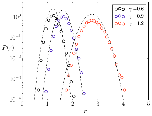
Figure 11: Steady state spatial pdf according to simulations of equations (22) with (2) as symbols and theory given by (32) as dashed lines. Parameter $\gamma$ given in the figure. Other parameters: $\sigma^{2}=0.01$, $v_{0}=1$, $\kappa=1$, $\alpha=2$.

This marginal pdf is compared with simulation results in figure 11. The colored symbols are obtained from simulations according to equations (22), with the definition of the position angle $\beta$, given by (2). The black dashed lines correspond to equation (32). The approximations (32) fit the simulation results well for the small noise intensity $\sigma^{2}=0.01$.

We remind that we selected $\gamma\in(0,\pi/2)$. A corresponding distribution can be derived with negative shifts if the stable fixpoint is located in the lower halfplane. In the Cartesian coordinate system both possess the same steady state pdf as circular symmetric crater-like distribution with radius $r_{*}$. The crater is accompanied by a homogeneous rotation around the home in an either clockwise $\gamma<0$, or counterclockwise $\gamma>0$ fashion.

III.2.2 Small Noise Strength: Steady State - $\alpha-$Stable White Noise

In this subsection we will discuss situations with $\alpha-$stable white noise sources being not Gaussian. This distinction seems appropriate for two reasons. First, the expansion for small $\delta_{z}$ is questionable for Non-Gaussian $\alpha$-stable white noise, as those processes are not continuous, they jump. So, an approximation for small $\delta_{z}$ does not consider jumps, it has to be done with caution. We do it anyway and will justify this by an agreement with simulation results, as presented later on. As we infere from the left graphs of Fig.(10), jumps are rare and lead to large excursions, so the approximation can still be usefull at the center of the pdf. Secondly, as was shown in Sokolov, Ebeling, and Dybiec (2011) the position and the velocity are coupled in a non trivial way for harmonic oscillators driven by Lévy noise, in general. Only for Gaussian white noise the resulting pdf can be written as product of the angular dynamics and the position dynamics Sokolov, Ebeling, and Dybiec (2011). We will find an approximation only for the marginal pdf of the position and then discuss the result in comparison with simulations.

Despite these initial warnings, we start the same as in the Gaussian white noise case with the dynamics obtained by expansion for small $\delta_{z}$ and $\delta_{r}$ given by (26) and (27). We write both equations as second derivative of the position $\delta_{r}$ with noise present

$$0=\ddot{\delta}_{r}+\sin(\gamma)\dot{\delta}_{r}+\cos^{2}(\gamma)\delta_{r}+\sigma\xi(t)\,,$$ (33)

for $\gamma>0$. We consider the overdamped regime. We look at time scales $t\gg(\sin(\gamma))^{-1}$ and eliminate the acceleration, leaving with

$$\dot{\delta}_{r}=-\frac{1}{\sin(\gamma)}\left(\cos^{2}(\gamma)\delta_{r}+\frac{\sigma}{v_{0}}\xi(t)\right)\,.$$ (34)

The noise is symmetric, so we can keep the plus sign in front of the noise term. Such equation (34) was solved and discussed in West and Seshadri (1982). We take their result for the asymptotic $t\rightarrow\infty$ and return to the coordinate $r$ and express the steady state spatial pdf for the distance through the Fourier transform

$$P_{0}(r)=\int_{-\infty}^{\infty}\,{\rm{d}}k\,\exp\left(-ik\left(r-\frac{1}{\cos(\gamma)}\right)\right)\exp\left(-\left(\frac{\sigma}{v_{0}}\right)^{\alpha}\frac{\sin(\gamma)}{\alpha\sin^{\alpha}(\gamma)\cos^{2}(\gamma)}|k|^{\alpha}\right)\,.$$ (35)

For the special case of Cauchy distributed white noise with $\alpha=1$ the result becomes

$$P_{0}(r)=\frac{\sigma}{\pi v_{0}}\frac{1}{\left(r\cos(\gamma)-1\right)^{2}+\left(\sigma/(v_{0}\cos(\gamma))\right)^{2}}$$ (36)

for the marginal steady state spatial density.

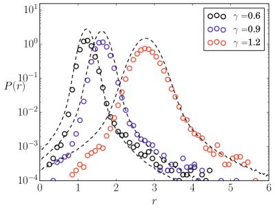
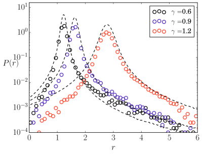
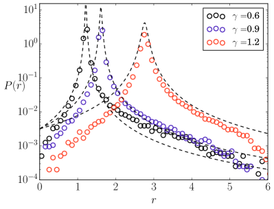
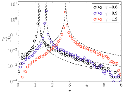
Figure 12: Marginal steady state spatial pdf according to simulations of equations (22) as symbols with $\beta$ defined in (2) and theory given by (32) as dashed lines. Top left: $\alpha=1.9$, Top right: $\alpha=1.5$, Bottom left: $\alpha=1.0$, Bottom right: $\alpha=0.5$. Parameter $\gamma$ given in the figure. Other parameters: $\sigma^{\alpha}=0.01$, $v_{0}=1$.

We compare in Fig. (12) the approximations (35), (36) with simulation results. The colored symbols are obtained from simulations according to equations (22), with the definition of the position angle $\beta$ given by (2). The black dashed lines correspond to equations (35), (36). The parameter $\gamma$ is given in the figures. The noise strength was chosen to be small $\sigma=0.01$. We took for the simulations $v_{0}=1$. We display in the top row the cases $\alpha=1.9$ (left) and $\alpha=1.5$ (right) and in the bottom row $\alpha=1.0$ (left) and $\alpha=0.5$ (right). While decreasing $\alpha$ the peak at $r_{*}$ becomes sharper and the tails become longer. The approximations fit generally rather well around the peak, but are better for larger $\alpha$ and smaller $\gamma$ values. For larger $\alpha$ values less jumps occur, so the approximation is expected to work better. As we expanded for small $\delta_{r}$ around $r_{*}$, the approximation does not reflect the tails correctly. A smaller $\gamma$ value corresponds to a stronger force around $r_{*}$, so if the angular variable experiences a jump and therefore the particle moves away from $r_{*}$, it returns faster for small $\gamma$, or slower for larger $\gamma$. This way it can be understood that the approximations work better for larger $\alpha$ and smaller $\gamma$.

Focussing on the simulation results of Figs. (11) and (12), we underline here, that the results of the pdf show close to the home higher values with decreasing $\alpha$, meaning that for Gaussian white noise the particle practically never is close to home (for instance $r=0.2$), while it has a larger probability density with $\alpha=0.5$. While we found that the mean first hitting time of a food source does not significantly depend on the noise type, in case the position angle is exactly known, we find here that for the return to the home part the noise type might matter, if an uncertainty of the position angle $\beta$ exists. Therefore a specific turning behavior of an observed animal might be related to the accuracy of its understanding of the surroundings and not to optimization of the search itself.

We remind that the distance $r$ was initially derived as polar representation of a two dimensional Cartesian system. As in the case of Gaussian noise, we ignored that distances can not be negative. In the simulations the density $P_{0}(r)$ approaches zero for vanishing $r$. It differs in our approximation and probability is also found at vanishing $r$ and below. Nevertheless, although some steps to derive the approximation (35) have to be taken with caution, the obtained approximations fit the simulations around the maximal values rather well and differences to the Gaussian cases become obvious.

Likewise in the Gaussian case, in the Cartesian coordinate system the steady state pdf for the distance is accompanied by a symmetric rotation around the home in an either clockwise $\gamma<0$, or counterclockwise $\gamma>0$ fashion.

III.2.3 Large Noise Strength

In the subsection, we derive the steady state spatial density for large noise strength $\sigma$. We will eliminate higher orders of the relaxation time $\tau=(v_{0}/\sigma)^{\alpha}$, as this time scale vanishes for $\sigma\rightarrow\infty$.

We start from the equation of motion for the dimensionless dynamics (23) containing $\gamma$ and wherein the position angle $\beta(t)$ is due to (2). Outgoing from this stochastic Langevin equation we formulate the corresponding FPE

$$\frac{\partial}{\partial t}P=-\cos(z)\frac{\partial}{\partial r}P-\frac{\partial}{\partial z}\left[\left(\cos(\gamma)-\frac{1}{r}\right)\sin(z)+\sin(\gamma)\cos(z)\right]P+\left(\frac{\sigma}{v_{0}}\right)^{\alpha}\frac{\partial}{\partial|z|^{\alpha}}P\,,$$ (37)

for the pdf $P=P(r,z,t|r_{0},z_{0},t_{0})$. We express the latter one through the angular $2\pi$ Fourier-transform with complex amplitudes

$$P_{n}(r,t)=\frac{1}{2\pi}\int_{-\pi}^{\pi}{\rm d}z\,\exp(-inz)P(r,z,t)\,.$$

Multiplying the FPE (37) from the left with $\exp(\text{i}nz)$ and integration over the angular variable $z$ leads to a set of linear equations for the Fourier amplitudes. We obtain the hierarchy:

$$\frac{\partial}{\partial t}P_{n} =-\frac{1}{2}\frac{\partial}{\partial r}\left(P_{n+1}+P_{n-1}\right)+\frac{n}{2}\left(\cos(\gamma)-\frac{1}{r}\right)\left(P_{n+1}-P_{n-1}\right)+$$ (38)

$$+\frac{\text{i}n}{2}\sin(\gamma)\left(P_{n+1}+P_{n-1}\right)-\left(\frac{\sigma}{v_{0}}\right)^{\alpha}|n|^{\alpha}P_{n}\,.$$

Being interested in the steady state, we set the l.h.s to zero, i.e. $\partial P_{n}/\partial t=0$, leaving:

$$\frac{|n|^{\alpha}}{\tau}P_{n} =-\frac{1}{2}\frac{\partial}{\partial r}\left(P_{n+1}+P_{n-1}\right)+\frac{n}{2}\left(\cos(\gamma)-\frac{1}{r}\right)\left(P_{n+1}-P_{n-1}\right)+$$ (39)

$$+\frac{\text{i}n}{2}\sin(\gamma)\left(P_{n+1}+P_{n-1}\right)\,,$$

with $\tau$ being the relaxation time from (20).

Further on, we find an approximative solution for large noise $\sigma$, respectively, for small $\tau$. The amplitudes with $n=0,\pm 1$ obey the two relations:

$$0=-\frac{1}{2}\frac{\partial}{\partial r}\left(P_{1}+P_{-1}\right)\,,$$ (40)

$$P_{\pm 1} =-\frac{\tau}{2}\frac{\partial}{\partial r}\left(P_{\pm 2}+P_{0}\right)+\frac{\tau}{2}\left(\cos(\gamma)-\frac{1}{r}\right)\left(P_{\pm 2}-P_{0}\right)+$$ (41)

$$\pm\frac{\text{i}\tau}{2}\sin(\gamma)\left(P_{\pm 2}+P_{0}\right)\,,$$

Insertion of $P_{\pm 1}$ into the first equation (40) yields

$$0 =-\frac{\tau}{4}\frac{\partial}{\partial r}\left\{\frac{\partial}{\partial r}2P_{0}+2\left(\cos(\gamma)-\frac{1}{r}\right)P_{0}+\right.$$ (42)

$$\left.+\left(\frac{\partial}{\partial r}-\cos(\gamma)+\frac{1}{r}\right)\left(P_{2}+P_{-2}\right)-i\sin(\gamma)\left(P_{2}-P_{-2}\right)\right\}\,.$$

The functions $P_{\pm 2}$ are of order $\tau P_{0}$. These functions become negligible as $\tau\rightarrow 0$. Hence, we find for large noise the steady state spatial density as:

$$P_{0}(r)=\cos^{2}(\gamma)r\exp(-\cos(\gamma)r)\,.$$ (43)

And thus, for large noise strength the steady state pdf becomes independent of the noise type and asymptotically independent of the noise strength $\sigma$.

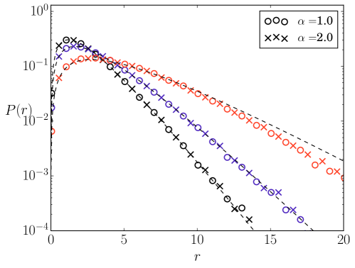
Figure 13: Marginal steady state spatial densities according to simulations with as symbols at high noise strength $\sigma^{\alpha}=4.0$. Symbol ’o’ corresponds to Cauchy distributed white noise $\alpha=1$ and symbol ’x’ to Gaussian white noise. The dashed lines are according to equation (43). Parameter $\gamma=0.6$ (black), $\gamma=0.9$ (blue) , $\gamma=0.9$ (red). Other parameters: $v_{0}=1$, $\kappa=1$.

Figure 13 shows simulation and theoretical results. Here, simulation results for Gaussian white noise (symbol x) and Cauchy distributed white noise (symbol o) are plotted for three different values of $\gamma$ and $\sigma^{\alpha}=4$. The marginal density remains dependent on $\gamma$ but does no longer depend on $\alpha$. The dashed lines in Fig. (13) correspond to the approximative solution (43). As can be seen, they fit the simulation results rather well.

This result is somewhat suprising. We introduced the shift $\gamma$, as an uncertainty of the position angle. We found that for small noise, the noise type can significantly increase the value of the pdf close to the home, the point where the particle wishes to return to. Now, we find that increasing the noise strength, and therefore changing the heading directions rather frequently drastically increases the pdf close to the home. As important result it implies the chances of returning to the home are significantly increased, as the running in circles motion is interrupted.

IV Conclusions

We resumed the study on a recently proposed stochastic model for a local searcher which is bound to a certain position called home Noetel et al. (2018). The search around and the return to the home is described by an uniform rule. It bases on an escape and pursuit interaction of the heading and the position vector. If both vectors point into the same direction the heading vector repels from the position vector in order to explore more space. Oppositely, if the heading vector points homewards, the two vectors align in order to find the home.

The model was composed with these properties to explain recent experimental findings with food searching fruit flies which perform stochastic oscillatory search around a given food position Kim and Dickinson (2017). In a recent publication Noetel et al. (2018) we showed the qualitative agreement with the experiment. However, the proposed model might be useful for much more applications of animal motion, for example, for explaining the search pattern of desert ants Wehner and Srinivasan (1981); Wehner, Michel, and Antonsen (1996); Vickerstaff and Merkle (2012), of general search Klages (2017) as well as technical applications like self-navigation of robots and social situations as mushrooming and orientation of visitors in unknown places and clients of supermarkets to find the exit.

Another main ingredient of the model was the constant speed $v_{0}$ of the searcher. We added noise only in the turning angle behavior as observed in the experiments with the fruit fly. Different white noise types as Gaussian and other stable Lévy noise was used as source of the randomness in the decision making of selecting a new heading direction. Interestingly, all different noise types with varying intensity did not have influence on the spatial density of searchers around the home.

Oppositely, the characteristic measure in the model which is affected by the noise is the mean time of finding a new localized food spot at a certain distance from the home. We reported on an optimal noise strength for finding this new spot in a minimal mean time $<t>$. It appeared to be the consequence of two counteracting effects driven by the noise. On the one side increasing noise populates stronger different orbits with probability. On the other side, a strong noise shrinks the influence of the deterministic motion which becomes replaced by low diffusion.

This optimal average time is distance dependent. The searcher finds on average the second spot always faster with noise in the angular dynamics. This is the result of the relaxation towards a probabilistic population of all possible trajectories which determines the greater success of the stochastic searcher. For lower noise this process is governed by the noisy periodic motion and after the relaxation time the stationary pdf is established. However, for larger noise the relaxation is proceeded by diffusive search.

In the second part, we discussed consequences of an erroneous observation of the position angle $\beta$ by the active particle. We did so by introducing an offset $\gamma$ in the interaction of heading and position vectors. We found that the resulting motion becomes circular around the home in Cartesian coordinates with the radius given by equation (24) if $|\gamma|\in(0,\pi/2)$. We obtained, that the spatial pdf depends on the noise type and its strength in case of small intensities. We approximated the spatial densities by linearizing the deterministic drift and discussed differences between white Gaussian and Cauchy $\alpha$-stable noise. In case of large noise again a noise independent distribution for the stochastic distances of the circular motion around the home was found.

We found, that while the mean first hitting time of a food source does not significantly depend on the noise type, that either noise type (for small noise strength), or noise strength (independent of the noise type) can increase the stationary pdf close to the home, if an uncertainty of the position angle exists. This finding might suggest that a specific in experiments observed turning behavior can be rooted in an uncertainty of the position angle and not in optimization of the time for finding a food source.

It would be more realistic to introduce time dependent process $\gamma(t)$ mimicking the forgetting of the actual direction of the home due to continued small errors. Such work is in progress. Also interacting searchers and their cooperative behavior are of central interest in future research.

V Acknowledgments

This work was supported by the Deutsche Forschungsgemeinschaft via grant IRTG 1740 and by the Sao Paulo Research Foundation (FAPESP) via grants 2015/50122-0 and 2017/04552-9. LSG thanks Dr. Alexander Neiman and Ohio University in Athens OH for hospitality and support. The authors thank Fabian Baumann and Bartlomiej Dybiec for fruitful discussions.

Appendix A Numerical Integration

The symmetric stable random variable $X$,with scale parameter $\sigma=1$, can be generated from uniform distributed random numbers $U_{1},\,U_{2}\in(0,1)$ Janicki and Weron (1994); Nolan (2018), by

$$V =\pi(U_{1}-1/2)$$

$$W =-\log(U_{2})$$

$$X =\left\{\begin{matrix}\frac{\sin{(\alpha V)}}{\cos{(V)^{1/\alpha}}}\left[\frac{\cos{((\alpha-1)V)}}{W}\right]^{(1-\alpha)/\alpha}&,\alpha\neq 1\\ \tan{(V)}&,\alpha=1\end{matrix}\right.$$ (44)

Considering Eq.(3), we perform the numeric integration by a deterministic Euler step with additional noise

$$\theta(t+\Delta t)=\kappa\sin(\theta-\beta)\Delta t+\frac{\sigma}{v_{0}}X_{1}\cdot\Delta t^{\frac{1}{\alpha}}+\theta(t)\,\,$$ (45)

with $X_{1}$ being a random variable drawn from a stable distribution. Due to the large tales in the pdf for the noise, we take a time step of $\Delta t=10^{-4}$.

Appendix B Fractional Derivative of Sine Functions

We show here, that the symmetric $\alpha$th Riesz-Weyl derivative for a sine function is the sine function with a pre-factor, see also Noetel, Sokolov, and Schimansky-Geier (2017). Considering the function $f(z)=\sin(b\,z)$, with $b$ being a real number and $z$ to be unwrapped $z\in(-\infty,\infty)$, the fractional derivative becomes

$$\frac{\partial^{\alpha}}{\partial|z|^{\alpha}}f(z)=-\frac{1}{4\,{\rm{i}}\,\pi}\int_{-\infty}^{\infty}\,{\rm{d}k}|k|^{\alpha}\,\exp\left(-ikz\right)\,\left(\delta(k+b)-\delta(k-b)\right)\,$$ (46)

where we included the Fourier transform of the sine function. Evaluating the $k$ integration leads to:

$$\frac{\partial^{\alpha}}{\partial|z|^{\alpha}}f(z)=-|b|^{\alpha}\,\sin(b\,z)\,.$$ (47)

References

- Bénichou et al. (2011) O. Bénichou, C. Loverdo, M. Moreau, and R. Voituriez, Rev. Mod. Phys. 83, 81 (2011).
- Klages (2017) R. Klages, “Search for food of birds, fish and insects,” in Diffusive Spreading in Nature, Technology and Society, edited by A. Bunde, J. Caro, J. Kärger, and G. Vogl (Springer, Cham, 2017) pp. 49–69.
- Mittelstaedt and Mittelstaedt (1980) M. Mittelstaedt and H. Mittelstaedt, Naturwissenwschaften 67, 566 (1980).
- Cheng (1995) K. Cheng, in Psychology of Learning and Motivation, Psychology of Learning and Motivation, Vol. 33 (Academic Press, 1995) pp. 1 – 21.
- Wang (2003) R. F. Wang, in Cognitive Vision, Psychology of Learning and Motivation, Vol. 42 (Academic Press, 2003) pp. 109 – 156.
- Seelig and Jayaraman (2015) J. D. Seelig and V. Jayaraman, Nature 521, 186 (2015).
- Green et al. (2017) J. Green, A. Adachi, K. K. Shah, J. D. Hirokawa, P. S. Magani, and G. Maimon, Nature 546, 101 (2017).
- Zeil (2012) J. Zeil, Cur. Opinion in Neurobiology 22,2, 285 (2012).
- Wehner, Michel, and Antonsen (1996) R. Wehner, B. Michel, and P. Antonsen, Journal of Experimental Biology 199, 129 (1996).
- el Jundi (2017) B. el Jundi, Current Biology 27, R748 (2017).
- Kim and Dickinson (2017) I. S. Kim and M. H. Dickinson, Current Biology 27, 2227 (2017).
- Wehner and Srinivasan (1981) R. Wehner and M. V. Srinivasan, Journal of Comparative Physiology A 142, 315 (1981).
- Vickerstaff and Merkle (2012) R. J. Vickerstaff and T. Merkle, Journal of Theoretical Biology 307, 1 (2012).
- Waldner (2018) F. Waldner, Journal of Comparative Physiology A ?, submitted for publication (2018).
- Vickerstaff and Di Paolo (2005) R. J. Vickerstaff and E. A. Di Paolo, in Advances in Artificial Life, edited by M. S. Capcarrère, A. A. Freitas, P. J. Bentley, C. G. Johnson, and J. Timmis (Springer Berlin Heidelberg, Berlin, Heidelberg, 2005) pp. 221–230.
- Mittelstaedt (1962) H. Mittelstaedt, Annual Review of Entomology 7, 177 (1962), https://doi.org/10.1146/annurev.en.07.010162.001141 .
- Chien and Wagstaff (2017) S. Chien and K. L. Wagstaff, Science Robotics 2 (2017).
- Hook et al. (2013) J. V. Hook, P. Tokekar, E. Branson, P. G. Bajer, P. W. Sorensen, and V. Isler, , 859 (2013).
- Girdhar et al. (2011) Y. Girdhar, A. Xu, B. B. Dey, M. Meghjani, F. Shkurti, I. Rekleitis, and G. Dudek, IEEE/RSJ , 5048 (2011).
- Leonard et al. (2007) N. Leonard, D. Paley, F. Lekien, R. Sepulchre, D. Fratantoni, and R. Davis, Proceedings of the IEEE 95, 48 (2007).
- Dubowsky et al. (2005) S. Dubowsky, K. Iagnemma, S. Liberatore, D. Lambeth, J. Plante, and P. J. Boston, Space Technology International Forum , 1449 (2005).
- Duarte et al. (2016) M. Duarte, V. Costa, J. Gomes, T. Rodrigues, F. Silva, S. M. Oliveira, and A. L. Christensen, PLOS ONE 11, 1 (2016).
- Nirmal and Lyons (2016) P. Nirmal and D. Lyons, Robotica 34, 2741 (2016).
- Möller et al. (2001) R. Möller, D. Lambrinos, T. Roggendorf, and R. P. R. Wehner, “Insect Strategies of Visual Homing in Mobile Robots,” in Biorobotics. Methods and Applications, edited by B. Webb and T. R. Consi (AAAI Press / MIT Press, 2001) pp. 37–66.
- Noetel et al. (2018) J. Noetel, V. L. Freitas, E. E. Macau, and L. Schimansky-Geier, Phys. Rev. E accepted for publication, (2018).
- Mikhailov and Meinköhn (1997) A. Mikhailov and D. Meinköhn, in Stochastic Dynamics, edited by L. Schimansky-Geier and T. Pöschel (Springer Berlin Heidelberg, Berlin, Heidelberg, 1997) pp. 334–345.
- Romanczuk et al. (2012) P. Romanczuk, M. Bär, W. Ebeling, B. Lindner, and L. Schimansky-Geier, Eur. Phys. J. Special Topics 202 (2012).
- Romanczuk, Couzin, and Schimansky-Geier (2009) P. Romanczuk, I. D. Couzin, and L. Schimansky-Geier, Phys. Rev. Lett. 102, 010602 (2009).
- Weron and Weron (1995) A. Weron and R. Weron, in Chaos — The Interplay Between Stochastic and Deterministic Behaviour, edited by P. Garbaczewski, M. Wolf, and A. Weron (Springer Berlin Heidelberg, Berlin, Heidelberg, 1995) pp. 379–392.
- Janicki and Weron (1994) A. Janicki and A. Weron, Simulation and Chaotic Behavior of Alpha-stable Stochastic Processes (Hugo Steinhaus Center, Wroclaw University of Technology, 1994).
- Nolan (2018) J. P. Nolan, Stable Distributions - Models for Heavy Tailed Data (Birkhauser, Boston, 2018) in progress, Chapter 1 online at http://fs2.american.edu/jpnolan/www/stable/stable.html.
- Nötel, Sokolov, and Schimansky-Geier (2017) J. Nötel, I. M. Sokolov, and L. Schimansky-Geier, Journal of Physics A: Mathematical and Theoretical 50, 034003 (2017).
- Ditlevsen (1999) P. D. Ditlevsen, Phys. Rev. E 60, 172 (1999).
- Schertzer et al. (2001) D. Schertzer, M. Larchevêque, J. Duan, V. V. Yanovsky, and S. Lovejoy, Journal of Mathematical Physics 42, 200 (2001), https://doi.org/10.1063/1.1318734 .
- Yanovsky et al. (2000) V. Yanovsky, A. Chechkin, D. Schertzer, and A. Tur, Physica A: Statistical Mechanics and its Applications 282, 13 (2000).
- Milster et al. (2017) S. Milster, J. Noetel, I. M. Sokolov, and L. Schimansky-Geier, Eur. Phys. J. Special Topics 226, 2093 (2017).
- Uhlenbeck and Ornstein (1930) G. E. Uhlenbeck and L. S. Ornstein, Phys. Rev. 36, 823 (1930).
- Sokolov, Ebeling, and Dybiec (2011) I. M. Sokolov, W. Ebeling, and B. Dybiec, Phys. Rev. E 83, 041118 (2011).
- West and Seshadri (1982) B. J. West and V. Seshadri, Physica A: Statistical Mechanics and its Applications 113, 203 (1982).
- Noetel, Sokolov, and Schimansky-Geier (2017) J. Noetel, I. M. Sokolov, and L. Schimansky-Geier, Phys. Rev. E 96, 042610 (2017).