11email: {pengbo7,tanwenming,lizheyang,zhangshun7,xiedi,pushiliang}@hikvision.com
Extreme Network Compression via Filter Group Approximation
Abstract
In this paper we propose a novel decomposition method based on filter group approximation, which can significantly reduce the redundancy of deep convolutional neural networks (CNNs) while maintaining the majority of feature representation. Unlike other low-rank decomposition algorithms which operate on spatial or channel dimension of filters, our proposed method mainly focuses on exploiting the filter group structure for each layer. For several commonly used CNN models, including VGG and ResNet, our method can reduce over 80% floating-point operations (FLOPs) with less accuracy drop than state-of-the-art methods on various image classification datasets. Besides, experiments demonstrate that our method is conducive to alleviating degeneracy of the compressed network, which hurts the convergence and performance of the network.
Keywords:
Convolutional Neural Networks, Network Compression, Low-rank Decomposition, Filter Group Convolution, Image Classification1 Introduction
In recent years, CNNs have achieved great success on several computer vision tasks, such as image classification [19], object detection [27], instance segmentation [25] and many others. However, deep neural networks with high performance also suffer from a huge amount of computation cost, restricting applications of these networks on the resource-constrained devices. One of the classic networks, VGG16 [30] with 130 million parameters needs more than 30 billion FLOPs to classify a single 224224 image. The heavy computation and memory cost can hardly be afforded by most of embedding-systems on real-time tasks. To address this problem, lots of studies have been proposed during last few years, including network compressing and accelerating [4, 5, 21, 41], or directly designing more efficient architectures [10, 14, 37, 40].
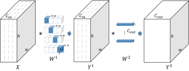
Low-rank decomposition is a common method to compress network by matrix or tensor factorization. A series of works [4, 16, 38, 41] have achieved great progress on increasing efficiency of networks by representing the original weights as a form of low-rank. However, these methods couldn’t reach an extreme compression ratio with good performance since they may suffer from degeneration problem [26, 29], which is harmful for the convergence and performance of the network. Filter group convolution [19] is another way to compact the network while keeping independencies among filters, which can alleviate the limitation of degeneration. In this work, we will show a novel method, which decompose a regular convolution to filter group structure [14] (Fig. 1), while achieve good performance and large compression ratio at the same time.
The concept of filter group convolution was first used in AlexNet [19] due to the shortage of GPU’s memory. Surprisingly, independent filter groups in CNN learned a separation of responsibility, and the performance was close to that of corresponding network without filter groups, which means this lighter architecture has an equal ability of feature representation. After this work, filter group and depthwise convolution were widely used in designing efficient architectures [2, 10, 14, 28, 37, 40] and achieved state-of-the-art performance among lightweight models. However, all of those well-designed architectures need to be trained from scratch with respect to specific tasks. Huang et al.[12] introduced CondenseNet, which learns filter group convolutions automatically during the training process, while several complicated stages with up to 300 epochs’ training are needed to reach both sparsity and regularity of filters.
In this paper, we will show an efficient way to decompose the regular convolutional layer into the form of filter group structure which is a linear combination of filter group convolution and point-wise convolution (Fig. 1). Taking advantage of filter group convolution, computational complexity of the original network can be extremely compressed while preserve the diversity of feature representation, which leads to faster convergence and less accuracy drop. Besides, our method can be efficiently applied on most of regular pre-trained models without any additional training skill.
The contributions of this paper are summarized as follows:
-
•
A filter group approximation method is proposed to decompose a regular convolutional layer into a filter group structure with tiny accuracy loss while mostly preserve feature representation diversity.
-
•
Experiments and discussions provide new inspiration and promising research directions based on degeneracy problem in network compression.
2 Related Work
First of all, we briefly discuss related works including network pruning, low-rank decomposition and efficient architecture designing.
Network pruning: Network pruning is an efficient method to reduce the redundancy in the deep neural network [31]. A straight forward way of pruning is to evaluate the importance of weights (e.g. the magnitude of weights [6, 21], sparsity of activation [11], Taylor expansion [24], etc.), thus the less important weights could be pruned with less effect on performance. Yu et al. [39] proposed a Neuron Importance Score Propagation algorithm to propagate the importance scores to every weight. He et al. [9] utilized a Lasso regression based channel selection and least square reconstruction to compress the network. Besides, there are several training-based studies in which the structure of filters are forced to sparse during training [22, 35]. Recently, Huang et al. [12] proposed an elaborate scheme to prune neuron connection with both sparsity and regularity during training process.
Low-rank decomposition: Instead of removing neurons of network, a series of works have been proposed to represent the original layer with low-rank approximation. Previous works [4, 20] applied matrix or tensor factorization algorithms (e.g. SVD, CP-decomposition) on the weights of each layer to reduce computational complexity. Jaderberg et al. [16] proposed a joint reconstruction method to decompose filter into a combination of and filters. These methods only gain limited compressions on shallow networks. Zhang et al. [41] improved the low-rank approximation of deeper networks on large dataset using a nonlinear asymmetric reconstruction method. Similarly, Masana et al. [23] proposed a domain adaptive low-rank decomposition method, which took the activations’ statistics of the new domain into account. Alvarez et al. [1] regularized parameter matrix to low-rank during training, such that it could be decomposed easily in the post-processing stage.
Efficient architecture designing: The needs of applying CNNs on resource-constrained devices also encouraged the studies of efficient architecture designing. ‘Residual’ block in ResNet [7, 8], ‘Inception’ block in GoogLeNet [32, 33, 34] and ‘fire module’ in SqueezeNet [13] achieved impressive performance with less complexity on spatial extents. AlexNet [19] utilized filter group convolution to solve the constraints of computational resources. ResNeXt [37] replaced the regular convolutional layers in residual blocks of ResNet with group convolutional layers to achieve better results. Depthwise separable convolution proposed in Xception [2] promoted the performance of low-cost CNNs on embedded devices. Benefiting from depthwise separable convolution, MobileNet v1 [10], v2 [28] and ShuffleNet [40] achieved state-of-the-art performance on several tasks with significantly reduced computational requirements.
3 Approaches
In this section we introduce a novel filter group approximation method to decompose a regular convolutional layer into the form of filter group structure. Furthermore, we discuss the degeneracy problem of the compressed network.
3.1 Filter Group Approximation of Weights
Weights of convolutional layer can be considered as tensor , where and are the number of output channels and input channels respectively, and is the spatial size of filters. The response is computed by applying on which is sampled from sliding window of the layer inputs. Thus the convolutional operation can be formulated as:
| (1) |
The bias term is omitted for simplicity. and can be seen as matrices with shape -by-() and ()-by- respectively. The computational complexity of Eqn. 1 is .
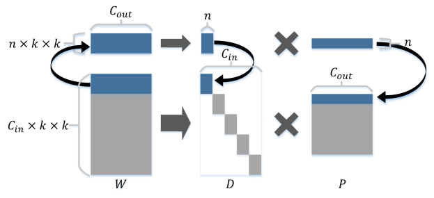
Each row of matrix is only multiplied with the corresponding column of matrix . Let’s consider each sub-matrix with rows of and columns of ( is divisible by ), which are denoted as and () respectively. Eqn. 1 can be equally described as:
| (2) |
Each sub-matrix with rank can be decomposed into two matrices and using SVD. Considering the redundancy of parameter in a layer, can be approximated by with rank . and are the first columns of and related to the largest singular values. By arranging and from each sub-matrices of into two matrices denoted as and respectively, we can get an approximation of matrix which is (Fig. 2). The original layer with weights can be replaced by two layers with weights and respectively. Thus the original response can be approximated by with:
| (3) |
| layer name | output size | ResNet34 | Ours-Res34/A | Ours-Res34/B | Ours-Res34/C | Ours-Res34/D |
|---|---|---|---|---|---|---|
| conv1 | - | |||||
| conv2_x | - | |||||
| conv3_x | - | |||||
| conv4_x | - | |||||
| conv5_x | - | - | ||||
| fc | - | |||||
| FLOPs | ||||||
The matrix is a block diagonal matrix as illustrated in Fig. 2, which can be implemented using a group convolutional layer with filters of spatial size , and each filter convolve with input channels sequentially. is a convolutional layer to create a linear combination of the output of . So the computational complexity of Eqn. 3 is . Compare with Eqn. 1, the complexity reduces to . It shrinks to about of the original one in the case of , which is known as depthwise convolution.
3.2 Reconstruction and Fine-tuning for the Compressed Network
Since our approximation is based on sub-matrices of , the accumulative error and magnitude difference among approximated sub-matrices will damage the overall performance. Hence we further minimize the reconstruction error by:
| (4) |
where indicates the response of the original network, and is the response after approximation. Eqn. 4 is a typical linear regression problem without any constrains which can be solved by the least-square optimization. Matrix can be implemented as a convolutional layer, which can be merged into in practice, thus there is no additional layer.
After reconstruction for each layer, the compressed network can maintain good performance even without fine-tuning. In our experiments, few epochs’ fine-tuning (usually less than 20 epochs) with a very small learning rate is enough to achieve better accuracy.

3.3 Compression Degree for Each Layer
When compressing an entire network, a proper compression ratio need to be determined for each layer. One common strategy is removing the same proportion of parameters for each layer. However, it is not reasonable since different layers are not equally redundant. As mentioned by [9, 41], deeper layers have less redundancy, which indicates less compression with increasing depth in whole network compression.
In our method, the compression ratio is controlled by n (see Section 3.1). For a whole network compression, we set larger n for deeper layers. Convolutional layers of the whole network can be separated into several stages according to the spatial size of corresponding output feature. Taking the experience of [14] for reference, we set the same n for those layers in the same stage, and the ratio of two values of n between adjacent stages is (shallow one vs deep one). Table 1 shows settings of n for each stage of ResNet34 in whole network compression, and ‘Ours-Res34/D’ is a ‘depthwise’ compressed case in which n for all stages is 1. We will further discuss different degrees of compression with network depth in our experiment.
3.4 Consideration about the Degeneracy Problem
As mentioned in [29], the Jacobian of weights indicates the correlation between inputs and outputs, and degeneracy of Jacobian leads to poor backpropagation of gradients which impacts the convergence and performance of the network. Jacobian can be computed as: , where and are inputs and outputs respectively. For linear case of two layers with weights and , the Jacobian .
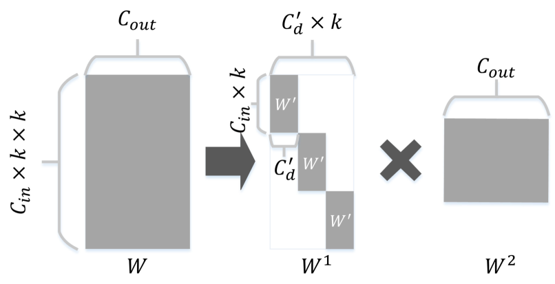
Low-rank decomposition method achieves compression by representing the original layer with a linear combination of several layers on a low-rank subspace. Fig. 3 illustrates two common low-rank decomposition strategies that decompose the weight matrix into two matrices and . and are numbers of input and output channels respectively, is the spatial size of filters. Let’s consider the case that , which is common in regular convolutional layers of classic networks like VGG [30], ResNet [7].
Fig. 3 shows an instance of SVD based method [41, 23]. The first singular vectors are reserved in SVD. Thus the rank of Jacobian is ,111We suppose that weight matrices after decomposition are full-rank which always holds in practice. and the computational complexity of the low-rank representation is . While in our method (Fig. 2), the rank can reach to no matter how much the model is compressed, and the computational complexity is . Under the same compression ratio, we can get:
| (5) |
Since , . Eqn. 6 shows that, the more the model is compressed, the less is, making the Jacobian more degenerate.
Jaderberg et al. [16] proposed a joint reconstruction method to represent a filter with two and filters, which is equivalent to the representation of Fig. 3. is the weight matrix of the convolutional layer with output channels. The rank of Jacobian is , and the computational complexity is . Similarly, under the same compression ratio,
| (6) |
When , , which means the compressed network from [16] degrades more quickly than ours as the compression ratio increases.
4 Experiments
In this section, a set of experiments are performed on standard datasets with commonly used CNN networks to evaluate our method. Our implementations are based on Caffe [17].
| Method | FLOPs | Top-1 |
|---|---|---|
| Ours-VGG16(S)/A | 40.03% | -0.39% |
| Asym. [41] (Fine-tuned, our impl.) | 39.77% | 0.28% |
| Liu et al. [22] | 37.00% | -0.22% |
| Ours-VGG16(S)/B | 73.40% | 0.02% |
| Asym. (Fine-tuned, our impl.) | 73.21% | 1.03% |
| Liu et al. | 67.30% | 2.34% |
| Ours-VGG16(S)/C | 84.82% | 0.57% |
| Asym. (Fine-tuned, our impl.) | 84.69% | 2.94% |
| Liu et al. | 83.00% | 3.85% |
| Ours-VGG16(S)/D | 88.58% | 1.93% |
| Asym. (Fine-tuned, our impl.) | 87.33% | 4.47% |
| Liu et al. 222Liu et al has not provided result with compression ratio about 88% . | - | - |
| Network | Method | FLOPs | Top-1 | Top-5 |
|---|---|---|---|---|
| VGG16 | Ours-VGG16/A | 56.99% | -0.82% | -0.94% |
| Asym. (Fine-tuned, our impl.) | 56.17% | -0.18% | -0.27% | |
| He et al. [9] | 50% | - | 0.0% | |
| Ours-VGG16/B | 77.86% | 0.28% | 0.07% | |
| Asym. (Fine-tuned, our impl.) | 77.60% | 1.81% | 0.73% | |
| Asym. (3D) [41] | 75% | - | 0.3% | |
| He et al. | 75% | - | 1.0% | |
| He et al. (3C) [9] | 75% | - | 0.0% | |
| Jaderberg et al. [16] ([41]’s impl.) | 75% | - | 9.7% | |
| Ours-VGG16/C | 81.35% | 1.06% | 0.27% | |
| Asym. (Fine-tuned, our impl.) | 81.18% | 4.53% | 2.45% | |
| Asym. (3D) | 80% | - | 1.0% | |
| He et al. | 80% | - | 1.7% | |
| He et al. (3C) | 80% | - | 0.3% | |
| Kim et al. [18] | 79.72% | - | 0.5% | |
| Ours-VGG16/D | 85.80% | 3.49% | 2.03% | |
| Asym. (Fine-tuned, our impl.) | 83.91% | 6.96% | 5.14% | |
| Asym. (3D) (Fine-tuned, our impl.) | 84.44% | 4.51% | 2.89% | |
| He et al. (3C) | 85.55% | 4.38% | 2.96% | |
| ResNet34 | Ours-Res34/A | 45.63% | 0.35% | 0.04% |
| Li et al. [21] | 24.20% | 1.06% | - | |
| NISP-34-B [39] | 43.76% | 0.92% | - | |
| Asym. (Fine-tuned, our impl.) | 44.60% | 0.97% | 0.21% | |
| Ours-Res34/B | 64.75% | 1.02% | 0.30% | |
| Li et al. (Fine-tuned, our impl.) | 63.98% | 4.35% | 2.29% | |
| Asym. (Fine-tuned, our impl.) | 64.12% | 2.91% | 1.41% | |
| Ours-Res34/C | 80.33% | 1.70% | 0.44% | |
| Li et al. (Fine-tuned, our impl.) | 79.67% | 8.23% | 4.96% | |
| Asym. (Fine-tuned, our impl.) | 79.95% | 6.77% | 4.10% | |
| Asym. (3D) (Fine-tuned, our impl.) | 80.08% | 3.79% | 1.85% | |
| Ours-Res34/D | 84.84% | 3.03% | 1.22% | |
| Li et al. (Fine-tuned, our impl.) | 84.99% | 13.27% | 8.84% | |
| Asym. (Fine-tuned, our impl.) | 84.79% | 12.30% | 8.27% | |
| Asym. (3D) (Fine-tuned, our impl.) | 84.04% | 5.35% | 2.78% |
| Network | Methods | FLOPs | Top-5 | GPU | CPU | TX1 |
|---|---|---|---|---|---|---|
| VGG16 | baseline | - | - | 2.91 | 2078 | 122.36 |
| Ours | 85.80% | 2.03% | 2.17 | 628 | 40.92 | |
| Asym.(3D) | 84.44% | 2.89% | 1.78 | 778 | 97.36 | |
| He et al.(3C) | 85.55% | 2.96% | 1.65 | 741 | 94.27 | |
| ResNet34 | baseline | - | - | 0.75 | 442 | 20.5 |
| Ours | 84.84% | 1.22% | 0.62 | 116 | 9.54 | |
| Asym.(3D) | 84.04% | 2.78% | 0.67 | 128 | 18.33 |
4.1 Datasets and Experimental Setting
Focusing on the reduction of FLOPs and accuracy drops, we compare our method with training from scratch and several state-of-the-art methods on CIFAR100 and ImageNet-2012 datasets [3] for image classification task.
CIFAR100 dataset contains 50,000 training samples and 10,000 test samples with resolution from 100 categories. We use a standard data augmentation scheme [7] including shifting and horizontal flipping in training. A variation of the original VGG16 from [22] (called VGG16(S) in our experiments) with top-1 accuracy 73.26% is used to evaluate the compression on CIFAR100 dataset.
ImageNet dataset consists of 1.2 million training samples and 50.000 validation samples from 1000 categories. We resize the input samples with short-side 256 and then adopt crop (random crop in training and center crop in testing). Random horizontal flipping is also used in training. We evaluate single-view validation accuracy. On ImageNet dataset, we adopt the compression on VGG16 [30] and ResNet34 [7].
4.2 Comparison with Training-from-scratch and Existing Methods
4.2.1 Comparison with Training-from-scratch
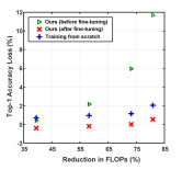
Several compression ratios are adopted in our experiments to evaluate the performance. For the fine-tuning processes of the compressed networks, we use an initial learning rate of 1e-4, and divide it by 10 when training losses are stable. epochs are enough for fine-tuning to achieve convergence. For comparison, we directly train models with the same architecture as our compressed networks from scratch for more than 100 epochs, with the same initialization and learning strategies as proposed by the original works [7, 30].
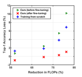
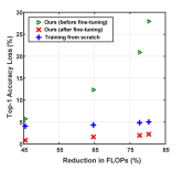
Comparison results are shown in Fig. 4. With 57% reduction of FLOPs for VGG16, the compressed network without fine-tuning only has a tiny accuracy loss on ImageNet, and it’s comparable to the performance of the scratch counterpart. With a few epochs’ fine-tuning, the compressed networks outperform training from scratch by a large margin. In some cases, our method even achieves higher accuracy than the original network.
4.2.2 Comparison with Existing Methods
Next, we compare our method with several state-of-the-art methods under the same compression ratios. To be noted, results demonstrated in our experiments are all fine-tuned.
As shown in Table 2, for VGG16(S) on CIFAR100, 4 compressed architectures (‘Ours-VGG16(S)/A,B,C,D’) are created by using different n as mentioned in Section 3.3. ‘Ours-VGG16(S)/A’ increases top-1 accuracy by 0.39% with 40% FLOPs reduction, which is slightly better than the other two methods. Under larger compression ratios, our method outperforms the other two methods with much lower accuracy loss. With 88.58% reduction of FLOPs (8.5 speed-up), the increased error rate of ‘Ours-VGG16(S)/D’ is 1.93% while Asym.’s is 4.47% under a similar compression ratio.
Networks trained on Imagenet with complex features are less redundant, which make compressing such networks much more challenging. The results of VGG16, ResNet34 and ResNet50 on ImageNet are shown in Table 3.
For VGG16, we adopt architectures ‘Ours-VGG16/A,B,C,D’ with respect to 4 compression ratios. With 56.99% reduction of FLOPs, the top-5 accuracy of ‘Ours-VGG16/A’ is 0.94% higher than the original network. When we speed the network up to , ‘Ours-VGG16/D’ can still achieve result of 2.03% top-5 accuracy drop, while for Asym. [41], it is much larger (5.14% drop on top-5 accuracy). Asym. (3D) and He et al. (3C) [9] improve their accuracy under the same compression ratios by combining with spatial decomposition [16]. However, the compressed architectures from combined methods are much inefficient on most of real-time devices since the original convolutional layer is decomposed into three layers with spatial filter size , and . Besides, the combination can be also applied on our method. We will conduct the exploration in our future work.
For ResNet34, the advantages in previous experiments still hold. ‘Ours-Res34/A’ reduces 45.63% of FLOPs with negligible accuracy drop. As the compression ratio increases, the performance of our method degrades very slowly. ‘Ours-Res34/D’ achieves 1.22% top-5 accuracy loss with 84.84% FLOPs reduction ( speed-up), while Li et al. [21] and Asym. suffer rapidly increased error rate. Similar to the results of VGG16, the combined Asym. (3D) outperforms Asym. a lot, but it is still worse than ours.
4.3 Actual Speed up of the Compressed Network
We further evaluate the actual running time of the compressed network. Table 4 illustrates time cost comparisons on different devices including Nvidia TITAN-XP GPU, Xeon E5-2650 CPU and Nvidia Jetson TX1. Due to the inefficient implementation of group operation in Caffe-GPU, our method shows large time cost. However, in most of resource-constrained devices, like CPU and TX1, bandwidth becomes the main bottleneck. In such case, our method achieves much significant actual speed up as shown in Table 4.
4.4 Compression Degree with Network Depth
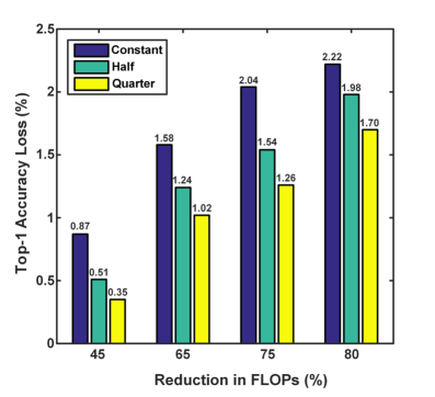
As mentioned in Section 3.3, the ratio of between adjacent stages is (hereinafter called ‘Quarter’) in our experiments. In this part, we consider another two degrees of compression. The first one is ‘Constant’, which means the n for all stages maintain the same. The second one is ‘Half’, which means the ratio of n between adjacent stages is . We evaluate these three kinds of strategies on compression of ResNet34. Fig. 5 illustrates the results. Compressed networks with ‘Quarter’ degree give the best performance, which is consistent with [14]. These results also indicate that there should be less compression with increasing depth.
4.5 Degeneracy of the Extremely Compressed Network
Fine-tuning is a necessary process to recover the performance of a compressed network. However fine-tuning after low-rank decomposition may suffer from the instability problem [20]. In our experiments for VGG16 on ImageNet, the training of compressed models from Asym. shows gradient explosion problems, which was also mentioned in [41]. Besides, the performance degraded quickly when the compression ratio was getting larger. This phenomenon is caused by the degeneracy of the compressed network [26, 29, 36].
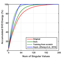
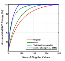
As we analyzed in Section 3.4, we calculate the singular values of Jacobian to analysis the degeneracy problem. Fig. 6 illustrates SVD accumulative curves of two layers from the original VGG16 and compressed networks ( speed-up) from Asym., our method and training from scratch with the same architecture as our compressed model. The curves of the original network (denotes as red solid lines) are the most flat, indicate the least degenerate. Ours (green solid) are the second, training from scratch (green dotted) and Asym. (blue solid) are worse than ours. The rest layers hold similar phenomena. Thus it can be concluded that, our proposed method can alleviate the degeneracy problem efficiently, while Asym. is much affected due to more elimination of singular value. The result also proves that training from scratch can not provide enough dynamic to conquer the problem of degeneracy [36].
The problems of training instability are lightened in ResNet due to the existence of Batch Normalization [15] and short-cut connection [26]. However the performance of Asym. on ResNet still degraded quickly as the compression ratio increased. The degeneracy of network is still an open problem. We believe that it should be taken into account when studying network compression.
4.6 A Better Initialization of the Network
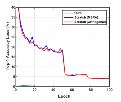
The comparison between training from scratch and our approximation method indicates that our compressed models provided a better initialization. For a further verification, we also evaluate the orthogonal initialization which could alleviate degeneracy in linear neural networks [29]. We compare models trained with the architecture of ‘Ours-Res34/A’. Fig. 7 illustrates the learning curves. Our compressed network achieves much lower accuracy loss.
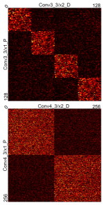
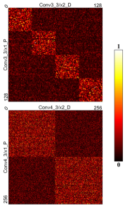
To give a better understanding, we conduct the inter-layer filter correlation analyses [14]. Fig. 8 shows the correlation between the output feature maps of filter group convolution and its previous point-wise convolution. Enforced by the filter group structure, the correlation shows a block-diagonal matrix. Pixels in the block-diagonal part of ours (Fig. 8(a)) are brighter than those of training from scratch (Fig. 8(b) and 8(c)), and reversed in the background. It means features between groups are more independent in our method. Similar phenomena are observed in other layers, which confirm that our proposed method gives a better initialization of the network.

5 Conclusion
In this paper, we proposed a filter group approximation method to compress networks efficiently. Instead of compressing the spatial size of filters or the number of output channels in each layer, our method is aimed at exploiting a filter group structure of each layer. The experimental results demonstrated that our proposed method can achieve extreme compression ratio with tiny loss in accuracy. More importantly, our method can efficiently alleviate the degeneracy of the compressed networks. In the future, we will focus on solving the degeneracy problem on network compression.
References
- [1] Alvarez, J.M., Salzmann, M.: Compression-aware training of deep networks. In: Advances in Neural Information Processing Systems (2017)
- [2] Chollet, F.: Xception: Deep learning with depthwise separable convolutions. In: IEEE Conference on Computer Vision and Pattern Recognition (2017)
- [3] Deng, J., Dong, W., Socher, R., Li, L.J., Li, K., Li, F.F.: Imagenet: A large-scale hierarchical image database. In: IEEE Conference on Computer Vision and Pattern Recognition (2009)
- [4] Denton, E., Zaremba, W., Bruna, J., Lecun, Y., Fergus, R.: Exploiting linear structure within convolutional networks for efficient evaluation. In: Advances in Neural Information Processing Systems (2014)
- [5] Han, S., Mao, H., Dally, W.J.: Deep compression: Compressing deep neural networks with pruning, trained quantization and huffman coding. In: International Conference on Learning Representations (2016)
- [6] Han, S., Pool, J., Tran, J., Dally, W.: Learning both weights and connections for efficient neural network. In: Advances in Neural Information Processing Systems (2015)
- [7] He, K., Zhang, X., Ren, S., Sun, J.: Deep residual learning for image recognition. In: IEEE Conference on Computer Vision and Pattern Recognition (2016)
- [8] He, K., Zhang, X., Ren, S., Sun, J.: Identity mappings in deep residual networks. In: European Conference on Computer Vision (2016)
- [9] He, Y., Zhang, X., Sun, J.: Channel pruning for accelerating very deep neural networks. In: IEEE International Conference on Computer Vision (2017)
- [10] Howard, A.G., Zhu, M., Chen, B., Kalenichenko, D., Wang, W., Weyand, T., Andreetto, M., Adam, H.: Mobilenets: Efficient convolutional neural networks for mobile vision applications. arXiv:1704.04861 (2017)
- [11] Hu, H., Peng, R., Tai, Y.W., Tang, C.K.: Network trimming: A data-driven neuron pruning approach towards efficient deep architectures. arXiv:1607.03250 (2016)
- [12] Huang, G., Liu, S., Laurens, V.D.M., Weinberger, K.Q.: Condensenet: An efficient densenet using learned group convolutions. arXiv:1711.09224 (2017)
- [13] Iandola, F.N., Han, S., Moskewicz, M.W., Ashraf, K., Dally, W.J., Keutzer, K.: Squeezenet: Alexnet-level accuracy with 50x fewer parameters and¡ 0.5 mb model size. arXiv:1602.07360 (2016)
- [14] Ioannou, Y., Robertson, D., Cipolla, R., Criminisi, A.: Deep roots: Improving cnn efficiency with hierarchical filter groups. In: IEEE Conference on Computer Vision and Pattern Recognition (2017)
- [15] Ioffe, S., Szegedy, C.: Batch normalization: accelerating deep network training by reducing internal covariate shift. In: International Conference on International Conference on Machine Learning (2015)
- [16] Jaderberg, M., Vedaldi, A., Zisserman, A.: Speeding up convolutional neural networks with low rank expansions. In: British Machine Vision Conference (2014)
- [17] Jia, Yangqing, Shelhamer, Evan, Donahue, Jeff, Karayev, Sergey, Long, Jonathan: Caffe: Convolutional architecture for fast feature embedding. In: In ACM International Conference on Multimedia, MM 14 (2014)
- [18] Kim, Y.D., Park, E., Yoo, S., Choi, T., Yang, L., Shin, D.: Compression of deep convolutional neural networks for fast and low power mobile applications. In: International Conference on Learning Representations (2016)
- [19] Krizhevsky, A., Sutskever, I., Hinton, G.E.: Imagenet classification with deep convolutional neural networks. In: Advances in Neural Information Processing Systems (2012)
- [20] Lebedev, V., Ganin, Y., Rakhuba, M., Oseledets, I., Lempitsky, V.: Speeding-up convolutional neural networks using fine-tuned cp-decomposition. Computer Science (2015)
- [21] Li, H., Kadav, A., Durdanovic, I., Samet, H., Graf, H.P.: Pruning filters for efficient convnets. In: International Conference on Learning Representations (2017)
- [22] Liu, Z., Li, J., Shen, Z., Huang, G., Yan, S., Zhang, C.: Learning efficient convolutional networks through network slimming. In: IEEE International Conference on Computer Vision (2017)
- [23] Masana, M., Joost, V.D.W., Herranz, L.: Domain-adaptive deep network compression. In: IEEE International Conference on Computer Vision (2017)
- [24] Molchanov, P., Tyree, S., Karras, T., Aila, T., Kautz, J.: Pruning convolutional neural networks for resource efficient inference. In: International Conference on Learning Representations (2017)
- [25] Noh, H., Hong, S., Han, B.: Learning deconvolution network for semantic segmentation. In: IEEE International Conference on Computer Vision (2016)
- [26] Orhan, A.E., Pitkow, X.: Skip connections eliminate singularities. In: International Conference on Learning Representations (2018)
- [27] Ren, S., He, K., Girshick, R., Sun, J.: Faster r-cnn: Towards real-time object detection with region proposal networks. IEEE transactions on pattern analysis and machine intelligence 39(6), 1137–1149 (2017)
- [28] Sandler, M., Howard, A., Zhu, M., Zhmoginov, A., Chen, L.C.: Inverted residuals and linear bottlenecks: Mobile networks for classification, detection and segmentation. arXiv:1801.04381 (2018)
- [29] Saxe, A.M., Mcclelland, J.L., Ganguli, S.: Exact solutions to the nonlinear dynamics of learning in deep linear neural networks. In: International Conference on Learning Representations (2013)
- [30] Simonyan, K., Zisserman, A.: Very deep convolutional networks for large-scale image recognition. In: International Conference on Learning Representations (2015)
- [31] Srinivas, S., Babu, R.V.: Data-free parameter pruning for deep neural networks. In: British Machine Vision Conference (2015)
- [32] Szegedy, C., Ioffe, S., Vanhoucke, V., Alemi, A.: Inception-v4, inception-resnet and the impact of residual connections on learning. In: AAAI Conference on Artificial Intelligence (2017)
- [33] Szegedy, C., Liu, W., Jia, Y., Sermanet, P., Reed, S., Anguelov, D., Erhan, D., Vanhoucke, V., Rabinovich, A.: Going deeper with convolutions. In: IEEE Conference on Computer Vision and Pattern Recognition (2015)
- [34] Szegedy, C., Vanhoucke, V., Ioffe, S., Shlens, J., Wojna, Z.: Rethinking the inception architecture for computer vision. In: IEEE Conference on Computer Vision and Pattern Recognition (2016)
- [35] Wen, W., Wu, C., Wang, Y., Chen, Y., Li, H.: Learning structured sparsity in deep neural networks. In: Advances in Neural Information Processing Systems (2016)
- [36] Xie, D., Xiong, J., Pu, S.: All you need is beyond a good init: Exploring better solution for training extremely deep convolutional neural networks with orthonormality and modulation. In: IEEE Conference on Computer Vision and Pattern Recognition (2017)
- [37] Xie, S., Girshick, R., Dollar, P., Tu, Z., He, K.: Aggregated residual transformations for deep neural networks. In: IEEE Conference on Computer Vision and Pattern Recognition (2017)
- [38] Xue, J., Li, J., Gong, Y.: Restructuring of deep neural network acoustic models with singular value decomposition. In: Conference of the International Speech Communication Association (2013)
- [39] Yu, R., Li, A., Chen, C.F., Lai, J.H., Morariu, V.I., Han, X., Gao, M., Lin, C.Y., Davis, L.S.: Nisp: Pruning networks using neuron importance score propagation. arXiv:1711.05908 (2017)
- [40] Zhang, X., Zhou, X., Lin, M., Sun, J.: Shufflenet: An extremely efficient convolutional neural network for mobile devices. arXiv:1707.01083 (2017)
- [41] Zhang, X., Zou, J., He, K., Sun, J.: Accelerating very deep convolutional networks for classification and detection. IEEE transactions on pattern analysis and machine intelligence 38(10), 1943–1955 (2016)