The Haldane model under quenched disorder

Abstract

We study the half-filled Haldane model with Anderson and binary disorder and determine its phase diagram, as a function of the Haldane flux and staggered sub-lattice potential, for increasing disorder strength. We establish that disorder stabilizes topologically nontrivial phases in regions of the phase diagram where the clean limit is topologically trivial. At small disorder strength, our results agree with analytical predictions obtained using a first order self-consistent Born approximation, and extend to the intermediate and large disorder values where this perturbative approach fails. We further characterize the phases according to their gapless or gapped nature by determining the spectral weight at the Fermi level. We find that gapless topological nontrivial phases are supported for both Anderson and binary disorder. In the binary case, we find a reentrant topological phase where, starting from a trivial region, a topological transition occurs for increasing staggered potential $\eta$, followed by a second topological transition to the trivial phase for higher values of $\eta$.

I Introduction

Topological band insulators have been attracting a great deal of attention due to their unusual properties when compared to trivial, common band insulators (Hasan and Kane, 2010; Qi and Zhang, 2011; with Taylor L. Hughes, 2013; Chiu et al., 2016). After the discovery of the quantum Hall effect (Klitzing et al., 1980) and its theoretical explanation using concepts of topology (Thouless et al., 1982; Niu et al., 1985), the first proposal of a topological phase without the need of an applied homogeneous magnetic field was due to Haldane (Haldane, 1988). The quantum anomalous Hall effect predicted by Haldane was recently realized experimentally on several systems under zero net magnetic field (Chang et al., 2013; Jotzu et al., 2014; Checkelsky et al., 2014; Chang et al., 2015). This makes quantum anomalous Hall insulators, or Chern insulators according to the topological classification (Chiu et al., 2016), very interesting systems to study quantum topological matter at the fundamental level, and to explore possible technological applications of their distinctive feature – the protected, gapless surface states that run on the sample edges.

Topological systems are known to be robust to disorder effects (Xiao et al., 2010), meaning that the system’s topological properties can emerge even in the presence of disorder as long as it does not break any fundamental symmetry. In the case of quantum Hall systems and anomalous quantum Hall insulators, disorder is even crucial for the observation of quantized Hall conductivity, since it localizes every state except for those carrying the topological invariant (Kramer and MacKinnon, 1993; Onoda and Nagaosa, 2003; Onoda et al., 2007). A well quantized Hall plateau is then the consequence of the Fermi level laying in the gap (filled of localized states) which separates the extended states that carry the topological invariant. With increasing disorder strength a localization transition occurs, accompanied by a topological transition between a topological (Chern) insulator and a trivial (Anderson) insulator. As disorder increases, the bulk extended states above and below the Fermi level carrying the topological invariant shift toward one another and annihilate, leading to the topological phase transition into the trivial phase. The standard mechanism is referred to as “levitation and annihilation” of extended states (Onoda et al., 2007). Increasing disorder strength leads, generally, the Chern insulator to a trivial phase (Prodan et al., 2010; Prodan, 2011), although exceptions have recently been identified (Castro et al., 2015, 2016).

In 2009, Li et.al. surprisingly discovered that it was possible to obtain a topological phase transition from a topologically trivial phase to a topologically non-trivial phase with quantized conductance by increasing Anderson disorder (Li et al., 2009) - the now called topological Anderson insulator (TAI) phase. This phenomenon was latter explained by Groth et. al. with the usage of the a perturbative first order self-consistent Born approximation (Groth et al., 2009). The picture emerging from this low energy approach is that the trivial and non-trivial masses compete and the phenomenon can be understood as a renormalization of the trivial mass to lower values for increasing (although perturbative) disorder. Building on these seminal works several studies treated models supporting possible TAI phases, including the disordered Kane-Mele model (Kane and Mele, 2005; Orth et al., 2016) and the disordered Haldane model (Song et al., 2012; García et al., 2015). For the Kane-Mele model, the presence of a staggered potential was shown to be a necessary condition for the disorder-driven transition into the TAI phase and the energy window associated with a quantized non-zero conductance was verified to increase with the disorder strength in this case (Orth et al., 2016). In Ref. (Song et al., 2012), the Hall conductance was studied in the Anderson disorder - Fermi energy plane for the Haldane model and a TAI phase was found for a value of the staggered potential for which the topological phase is suppressed in the clean limit. In parallel with the disordered Kane-Mele model, it was also observed a disorder-driven increase of the energy window associated with the topological phase in the disordered Haldane model, in Ref. (García et al., 2015). The first order Born approximation was also applied to the Haldane model in this work, by mapping the corresponding low energy Hamiltonian into the low energy Hamiltonian of a HgTe quantum well. Other models with similar phenomenology include a two-dimensional semi-Dirac material (Sriluckshmy et al., 2018) and a model where the disorder is introduced through magnetic impurities (Raymond et al., 2015).

In the present paper we study the evolution of the total phase diagram of the Haldane model at half-filling with increasing disorder. Despite the knowledge accumulated on this model so far, a global phase diagram with indicating the gapped or gapless nature of the system at each point and its topological properties, is still lacking. Furthermore, we extend our study of the phase diagram to both Anderson and binary disorder, and show that interesting qualitative differences exist between them. Our aim is to understand how topological phases behave, not only for small disorder strength, for which topological properties are expected to be robust, but also for disorder strengths capable of destroying the topological features, thus shedding light on the robustness of TAI phases in the intermediate and strong disorder regimes where perturbative methods are not reliable. Our findings are relevant to understand Chern insulating phases in real systems where disorder is unavoidable. In particular, the striking similarity between the phase diagram we obtain for Anderson disorder and measurements of differential drift velocity for the Haldane model realized with cold fermionic atoms (Jotzu et al., 2014) suggests that disorder could, at least partially, account for the observed deviations from the result expected for clean systems.

The paper is organized as follows: In Sec. II, we introduce the Haldane model and specify the types of applied disorder. We also briefly explain the methods employed to obtain the results in Sec. III. In the latter, we present numerical results on the phase diagram of the disordered Haldane model, including the behavior of the topological phases up to the point they are suppressed and the gapped and gapless regions of the phase diagram. Sec. IV is dedicated to the discussion of the obtained results and in Sec. V the key results are summarized and some conclusions are drawn on their implications.

II Model and methods

We consider the Haldane model (Haldane, 1988) with Hamiltonian written as

$$H_{0}=-t\sum_{\left\langle i,j\right\rangle}c_{i}^{\dagger}c_{j}+t_{2}\sum_{\left\langle\left\langle i,j\right\rangle\right\rangle}e^{i\phi_{i,j}}c_{i}^{\dagger}c_{j}+\eta\sum_{i}\zeta_{i}c_{i}^{\dagger}c_{i},+\text{H.c}.,$$ (1)

where the disorder effects are induced by a site-dependent potential term

$$H=H_{0}+\sum_{i}\xi(i)c_{i}^{\dagger}c_{i}.$$ (2)

Here, $c_{i}^{\dagger}(c_{i})$ are creation (annihilation) operators defined in the two triangular sub-lattices $A$ and $B$ that form the honeycomb lattice. The first term in Eq. (1) corresponds to hopping between nearest neighbor sites $\langle i,j\rangle$, and couples sublattices $A$ and $B$. The second term describes complex next-to-nearest neighbor hopping between sites $\langle\langle i,j\rangle\rangle$, with amplitude $t_{2}e^{i\phi_{ij}}$ and $\phi_{ij}=\nu_{ij}\phi$, where $\nu_{ij}=(2/\sqrt{3})(\hat{\boldsymbol{d}}_{1}\times\hat{\boldsymbol{d}}_{2})=\pm 1$ with $\hat{\boldsymbol{d}}_{1}$ and $\hat{\boldsymbol{d}}_{2}$ two unit vectors along the two bonds connecting $\langle\langle i,j\rangle\rangle$. In the following $t$ is set to unity and $t_{2}=0.1t$ which ensures a direct gap with no band overlapping (Haldane, 1988). The third term corresponds to a staggered potential, where $\zeta_{i}=1$ if $i\in A$ and $\zeta_{i}=-1$ if $i\in B$. These last two terms are respectively responsible for breaking time-reversal and inversion symmetries and thus for opening non-trivial and trivial topological gaps at the Dirac points. In the absence of disorder the phase diagram of the Haldane model in the $(\eta,\phi)$ parameter space encompasses a trivial phase with vanishing Chern number and two topological non-trivial phases with $C=\pm 1$ respectively. The site-dependent potentials $\xi(i)$ are uncorrelated for different sites and follow the probability distribution

$$\begin{cases}P_{W}(\xi_{i})=\frac{1}{W}\Theta\left(\frac{W}{2}-\left|\xi_{i}\right|\right)&\text{Anderson},\\ P_{V}(\xi_{i})=\frac{1}{2}\left[\delta\left(\xi_{i}\right)+\delta\left(\xi_{i}+V\right)\right]&\text{binary},\end{cases}$$ (3)

where $W$ and $V$ parametrize the disorder strength for the Anderson and binary cases, respectively.

In the following, we extend the phase diagram of the Haldane model by increasing the disorder strength until the topological phases are destroyed. We identify the topological nature of each phase by computing the Chern number using Fukui’s method (Fukui et al., 2005) as implemented in Ref. (Zhang et al., 2013), a variant that is suitable to deal with disordered systems for which translational invariance is broken. The results are confirmed using the transfer matrix method (TMM) (Mackinnon and Kramer, 1981; MacKinnon and Kramer, 1983; Hoffmann and Schreiber, 2012) in the regions of the phase diagram where the density of states (DOS) is gapless for which results are trustworthy. The method considers a finite system with a fixed large longitudinal dimension $L$ and a transverse dimension of size $M$, which is varied in order to compute the localization length $\lambda_{M}$. We study the behavior of the normalized localization length $\Lambda_{M}=\lambda_{M}/M$ as a function of $M$: if $\Lambda_{M}$ decreases with $M$, the eigenstates are localized in the thermodynamic limit and therefore the system is an insulator; on the contrary, if $\Lambda_{M}$ increases with $M$, the eigenstates are extended and the system is metallic; a constant $\Lambda_{M}$ signals a critical point separating the two regimes. The longitudinal dimension $L$ was chosen to be of the order of $10^{6}$ to guarantee a relative error smaller than $1\%$ for $\lambda_{M}$. The DOS is obtained using a recursive Green’s function method (Ehrenreich et al., 1980; Haydock and Nex, 1984), allowing the access to system sizes in excess of $10^{6}$ lattice sites.

III Results

III.1 Phase diagram evolution

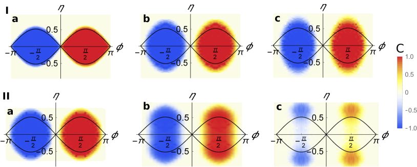
Figure 1: (I) Evolution of the phase diagram with Anderson disorder. a) $W/t=2$; b) $W/t=3.5$; c) $W/t=4$. The results in a) and b) were obtained for a system of size $12\times 12$ while the results in c) were for a $20\times 20$ system. A total of $100$ disorder configurations were used. (II) Evolution of the phase diagram with binary disorder. a) $V/t=2$; b) $V/t=2.4$; c) $V/t=2.75$. The results in a) were obtained for a $12\times 12$ system while the ones in figures b) and c) were obtained for systems of size $20\times 20$. The black curves correspond to the phase transition curves of the Haldane model with no disorder.

In this section we provide the evolution of the phase diagram with the disorder strength for the Anderson and binary cases. Figure 1(I) shows the evolution of the phase diagram for different disorder strengths $W$ in the Anderson case. The color code depicts the values of the Chern number and the black lines show the phase boundaries for the case with no disorder. For small disorder strength, the topological phases are robust and no significant change in the phase diagram is observed. For $W/t=2$, a small enhancement of the topological phases along the $\eta$ direction, shown in Fig. 1(Ia), can already be observed for values of $\phi$ near $\pm\pi/2$. This effect becomes very distinct for larger disorder strengths, as can be seen in Figs. 1(Ib) and 1(Ic) and is in accordance with the results obtained in Ref. (Sriluckshmy et al., 2018). Along with this phenomenon, the phases separate near $\phi=0$, becoming “squeezed” in the $\phi$ direction.

The evolution of the phase diagram for binary disorder is shown in Fig. 1(II). The same qualitative phenomena as for Anderson disorder is observed - an enhancement of the topological phases in the $\eta$ direction and “squeezing” in the $\phi$ direction, as can be seen in Figs 1(IIa) and 1(IIb). However, just before the topological phases are destroyed, a different phenomenon occurs: the last regions of the topological phases to disappear are for finite $\eta$ [see Fig. 1(IIc)], in contrast with the Anderson case for which this phenomenon does not occur. For Anderson disorder, the squeezing shown in Figs.  1(Ib) and 1(Ic) keeps going till the topological phase is concentrated on a thin region around $\phi\simeq\pm\pi/2$, including $\eta=0$, disappearing above a critical disorder $W_{c}/t\simeq 5.2$.

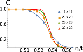
Figure 2: Example of the computed Chern numbers for different system sizes for Anderson disorder with $W/t=1$ and $\phi=\pi/2$. The standard deviation errors obtained by averaging over different disorder realizations are shown for each data point.

To inspect the enhancement of the topological phases in the $\eta$ direction more quantitatively, we study the $(W,\eta)$ phase diagram for $\phi=\pi/2$. We performed a finite size scaling analysis to check the convergence of the phase transition point at the thermodynamic limit. An average over 200 disorder configurations was always performed. For each system size, the data points were interpolated. The phase transition point was considered to be the intersection between the curves corresponding to the larger systems. An example of the obtained curves is provided in Fig. 2. Notice that the transition from $C=1$ to $C=0$ becomes sharper for larger system sizes, precluding the abrupt transition in the thermodynamic limit. The errors shown in Fig. 1 are associated with the intersection of the two cubic splines used to compute the phase transition points. Horizontal and vertical error bars were respectively obtained by varying the disorder strength with fixed $\eta$ and vice-versa.

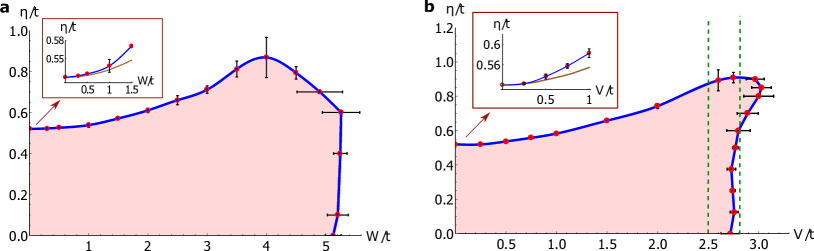
Figure 3: Phase diagram of the Haldane model with Anderson disorder in the $(W,\eta)$ plane (a) and with binary disorder in the $(V,\eta)$ plane (b), for $\phi=\pi/2$. The insets show a region of small disorder amplitude zoomed to highlight the comparison between the analytical predictions (brown curves), obtained with a first-order self-consistent Born approximation (see Appendix A), and the numerical results. The dashed green lines in (b) correspond to the cuts of the phase diagram analyzed with TMM in Fig. 4.

For Anderson disorder, the $(W,\eta)$ phase diagram at fixed $\phi=\pi/2$ is shown in Fig. 3(a) along with the perturbative results shown in the inset, obtained for the first order self-consistent Born approximation (see Appendix. A). The agreement between the perturbative result and the numerical calculation in the low disorder regime is indicative of the correctness of the later. For finite $W/t\lesssim 5.1$, the transition from the trivial insulating phase to the topological insulating one occurs for values of $\eta$ larger then those attained for the case of no disorder (where $\eta_{c}=3\sqrt{3}t_{2}$). This is a clear signature of the onset of a TAI phase, which extends well beyond the validity of the perturbative regime.

The $(V,\eta)$-phase diagram for binary disorder at fixed $\phi=\pi/2$ is shown in Fig. 3(b). The stabilization of the topological phase for values of $V$ higher than in the clean limit indicates the presence of a TAI phase also for binary disorder. This agrees with the result from the first order self-consistent Born approximation (see Appendix. A), and shows that, like for Anderson disorder, the TAI phase extends to intermediate values of disorder, beyond the perturbative result. At odds with Anderson disorder, however, a reentrant behavior is clearly seen in Fig. 3(b) for binary disorder. This form of the $(V,\eta)$ transition line confirms the phase diagram in the $(\phi,\eta)$-plane shown in Fig. 1(IIc), where it is clearly seen that the topological region at $\eta$ close to zero is destroyed by disorder effects before the regions at larger values of $\eta$.

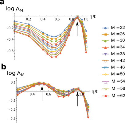
Figure 4: Results obtained with TMM for binary disorder $V/t=2.5$ (a) and $V/t=2.8$ (b) for systems with $M$-sites in the transverse direction and periodic boundary conditions. The normalized localization length $\Lambda_{M}$ decreases with $M$ except for the phase transition points for which this quantity remains unchanged. The single critical point obtained for $V/t=2.5$ and the two critical points obtained for $V/t=2.8$ are in accordance with the results obtained for the Chern number in Fig. 3(b).

III.2 Localization properties

The localization properties of disordered Chern insulators are well understood (Onoda and Nagaosa, 2003; Onoda et al., 2007; Xu et al., 2012). This model belongs to class A in the Altland-Zirnbauer symmetry classification (Altland and Zirnbauer, 1997; Evers and Mirlin, 2008), the same as quantum Hall insulators, where it is known that disorder localizes all states except those carrying the Chern number (with known exceptions when spin rotation is broken (Qiao et al., 2016; Su et al., 2016; Wang et al., 2015; Xu et al., 2012), which is not the case here). As disorder increases, the bulk extended states above and below the Fermi level carrying the topological invariant shift toward one another and annihilate, leading to the topological phase transition into the trivial phase through “levitation and annihilation” of extended states (Onoda et al., 2007). If we fix the energy to the point where the two extended states annihilate for some critical set of parameters $(W_{c},\eta_{c})$, the behavior with increasing disorder of the normalized localization length $\Lambda_{M}=\lambda_{M}/M$, obtained within the TMM, is as follows: for $W<W_{c}$ or $W>W_{c}$ the normalized localization length $\Lambda_{M}=\lambda_{M}/M$ decreases with $M$, as expected for localized states, while right at the transition point when $W=W_{c}$ the behavior $\Lambda_{M}=\text{const}$ is expected, characteristic of an extended (critical) state. Exactly the same behavior applies as a function of $\eta$ for fixed disorder. We may therefore use the TMM to independently confirm the phase diagram of Fig. 3 in the regions where the system is gapless (see Sec. III.3).

For the disordered Haldane model studied here, it can be shown that electron-hole symmetry is preserved at $\phi=\pi/2$. This guarantees that the Fermi level at half-filling coincides precisely with the energy where extended states meet and annihilate with increasing disorder or trivial mass $\eta$. Therefore, if we plot $\Lambda_{M}$ at the Fermi level as a function of $\eta$ the behavior described above is expected, and the points where $\Lambda_{M}$ does not change with $M$ should coincide with the phase transition lines in Fig. 3 obtained through the analysis of the topological invariant. Particularly relevant is the confirmation of the reentrant behavior found for binary disorder, shown in Fig. 3(b). Figure 4(a) shows that for $V/t=2.5$ there is a single value of $\eta\simeq 0.875$ for which $\Lambda_{M}$ becomes constant with increasing $M$ ranging from $M=22$ to $62$, signaling a phase transition. Away from the critical point, $\Lambda_{M}$ decreases with $M$, implying that the underlying phases are insulating. For $V/t=2.8$, Fig. 4(b) shows two transition points. Together, these findings confirm the scenario shown in Fig. 3(b) and further validate the values of the critical points obtained by exact diagonalization. We note that the quantum criticality of the Chern-to-trivial insulator transition has been analyzed in Ref. (Xue and Prodan, 2013) for Anderson disorder, and the same conclusions are expected to hold in the case of binary disorder.

III.3 Gapped and gapless regions of the phase diagrams

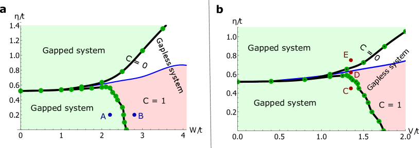
Figure 5: Characterization of the system spectral properties at the Fermi level in terms of its gapped or gapless nature as a function of parameters $(W,\eta)$ for Anderson disorder (a) and $(V,\eta)$ for binary disorder (b). We have fixed $\phi=\pi/2$. Thick (black) lines with circles separate gapped from gapless regions, while the thin (blue) line separates trivial from topological phases, as in the phase diagrams of Fig. 3. The computations were carried out for systems of size $1000\times 1000$. The DOS for the points A-E marked in this figure is shown in Fig. 6. The system was considered gapped whenever the DOS was below a threshold value of $0.1\%\epsilon$, where $\epsilon$ was chosen to be $\epsilon=1/\Delta E$, with $\Delta E=6t$ being the band width of the non-disordered system. Point coordinates: A=(2.2,0.2); B=(2.8,0.2); C=(1.35,0.45); D=(1.35,0.62); E=(1.35,0.75).

We now turn to the gapped or gapless nature of the spectrum at the Fermi level for the half-filled systems. In order to get this information, we computed the DOS at the Fermi level using the methodology referred in Sec. II. Figure 5 shows the phase diagram for $\phi=\pi/2$. The system was considered gapped whenever the DOS was below a threshold value of $0.1\%\epsilon$, where $\epsilon=1/\Delta E$ is a reference DOS value set to be the inverse bandwidth $\Delta E=6t$ of the non-disordered system. A variation of $\pm 10\%$ in this criterion showed not to change significantly the results. The obtained spectral characterization is qualitatively the same for Anderson [Fig. 5(a)] and binary [Fig. 5(b)] disorders. As expected, for small disorder the system is always gapped except at the topological transition line. This is seen in Fig. 5(a) and 5(b) whenever the gapped-gapless transition line (thick, black line with circles) coincides with the topological transition line (thin, blue line). However, for larger disorder, both trivial and topological regions become gapless and the topological phase transition is no longer associated to a spectral gap closing and re-opening.

Figure 5 is one of our main results, showing that topology and the presence or absence of a zero energy gap can be used to unravel the rich phase diagram of the disordered Haldane model.

Examples of the DOS within the different regions of the phase diagram are shown in Fig. 6 for the points labeled A-E in Fig. 5. For Anderson disorder, close inspection of the DOS at the Fermi level (zero energy) shows clearly [see inset in Fig. 6(a)] that in A the system is gapped while in B it is gapless. For binary disorder, where the Fermi level at half-filling occurs at the energy $V/2$, it is seen that while in points C and E the system is gapped [see inset in Fig. 6(b)], in point D it is clearly gapless.

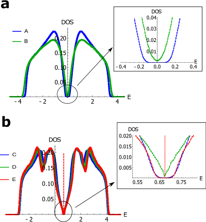
Figure 6: DOS for the points marked in Fig. 5 for Anderson (a) and binary (b) disorder. The insets show a zoomed region around $E=0$ for Anderson disorder and $V/2$ (corresponding to the red dashed line) for binary, which corresponds to the Fermi energy at half-filling in each case. An average over $25$ disorder configurations was considered and the error bars correspond to the standard deviation error associated to it. Systems of size $1000\times 1000$ were used.

IV Discussion

There are two notorious differences on how Anderson and binary disorder affect the topological phases: (i) a larger degree of disorder is necessary to destroy the topological phases in the Anderson case; and (ii) in the case of binary disorder, the last regions of the topological phases to be destroyed are for finite values of $\eta$, in contrast with the Anderson disorder case, where a topological non-trivial region around $\eta=0$ remains robust for higher disorder strength. These results are corroborated by TMM calculations and a first order Born approximation valid at small disorder strength.

Regarding the difference in the critical disorder needed to destroy the topological phase when we compare Anderson and binary disorder, we note that such difference remains even if we make the comparison in terms of the variance $\sigma^{2}$ of the respective disorder: Anderson $\sigma^{2}=W^{2}/12$ and binary $\sigma^{2}=V^{2}/4$ (see Appendix A). Without better explanation, we attribute this difference to the fact that Anderson disorder always includes configurations of small local potential, thus small disorder, as opposed to binary disorder for which the difference between site potentials is always either $0$ or $V$.

Arguably, the most salient difference between the two types of disorder is the reentrant behavior shown in Fig. 3(b) for binary disorder. Interestingly, if we fix $V\simeq 2.8t$, the reentrant topological phase shows up when the staggered potential $\eta$ starts to be comparable with $V/2$. A possible explanation for the effect would be the presence of some degree of cancellation of the two potentials, the staggered potential and the disorder potential, which would occur preferably for $\eta\sim V/2$.

The enhancement of the topological phases for moderate disorder strength is a clear signature of TAI: regions of the phase diagram that are trivial in a clean system are made topologically non-trivial by increasing the disorder strength. This effect is very robust as it is clearly seen for both types of disorder. For small disorder, an explanation based on the renormalization of the gap, as given by the perturbative treatment (see Appendix A), provides a reasonable understanding on the phenomenon. However, such explanation does not work at higher values of disorder since, after the spectral analysis shown in Fig. 5, the TAI regions become gapless for moderate disorder. More study is needed in order to understand the origin of the robustness of the TAI phase in this regime.

V Conclusions

We have studied the Haldane model under the influence of Anderson and binary disorder and obtained a comprehensive phase diagram for increasing the disorder strength up to the point when no topological phase survives. For both types of disorder, we obtained that the topological phases are enlarged along the staggered lattice potential strength, $\eta$, and “squeezed” along the flux $\phi$ direction.

In addition to the topological classification, the presence or absence of a spectral gap at the Fermi level was used to unravel the rich phase diagram of the disordered Haldane model, which has been shown to support four different phases: the gapped trivial and non-trivial topological phases that can be adiabatically connected to those of the clean system; and two gapless phases, either topologically trivial or not, that arise between the gapped ones for any finite value of disorder.

The fact that our simple example of a disordered Haldane model at half-filling already shows clear signatures of TAI phases at moderate to high disorder values is encouraging. We expect our findings to help guiding future attempts to realize disorder-induced topological non-trivial materials, and also to help in the understanding of Chern insulating phases in real systems where disorder is unavoidable. The Haldane model has already been experimentally realized in systems of ultracold fermions trapped in an optical lattice (Jotzu et al., 2014) and more recently its realization as a topological insulator laser was theoretically proposed (Harari et al., 2018). Moreover, the high controllability of system parameters in ultracold atoms (Roati et al., 2008) make them a very interesting test bed for disorder-induced phenomena and, in particular, to study how different kinds of disorder affect the topological phase. Indeed, the striking similarity between the phase diagram we obtained for Anderson disorder [Fig. 5(c)] and measurements of the differential drift velocity for the Haldane model realized in Ref. (Jotzu et al., 2014) suggests that disorder could at least partially account for the observed deviations from the expected result.

Appendix A Self-consistent Born approximation

In this section we show that the enhancement of the topological phases in the $\eta$ direction can be predicted perturbatively for small disorder strength by using the first order self-consistent Born approximation. This phenomenon is particularly noticeable for $\phi=\pi/2$, thus, in following, we consider only this case for simplicity. The low energy expansion of the Haldane Hamiltonian in momentum space around the two Dirac points, labeled $\bm{K}_{+}$ and $\bm{K}_{-}$, can be written as

$$H_{0}(\bm{k})=v(\tau_{z}\sigma_{x}k_{x}+\sigma_{y}k_{y})+\Big{[}\eta-\Big{(}3\sqrt{3}t_{2}-\frac{9\sqrt{3}}{4}t_{2}k^{2}\Big{)}\tau_{z}\Big{]}\sigma_{z}$$ (4)

where $v=3t/2$ is the Fermi velocity and $\bm{\sigma}$ and $\bm{\tau}$ are Pauli matrices that act respectively on the sub-lattice and the Dirac point’s pseudo-spin sub-spaces. As noticed in Ref. (Song et al., 2012), this Hamiltonian can be mapped into the low energy effective Hamiltonian of an HgTe quantum well, widely studied in the context of TAI (Li et al., 2009; Jiang et al., 2009; Groth et al., 2009). Following this set of works, we use the self-consistent Born approximation for which the self-energy can be determined by the self-consistent equation (Bruus and Flensberg, 2004):

$$\Sigma=\frac{3\sqrt{3}}{2}\Big{(}\frac{\sigma}{2\pi}\Big{)}^{2}\int_{\text{BZ}}\left\langle\Big{[}G_{0}^{-1}-\Sigma\Big{]}^{-1}\right\rangle$$ (5)

where $G_{0}^{-1}=E-H_{0}$ is the Green’s function of the unperturbed Hamiltonian, $\left\langle...\right\rangle$ denotes the disorder average and $\sigma^{2}$ is the variance of the disorder distribution,

$$\sigma^{2}=\begin{cases}W^{2}/12\,,&\text{Anderson disorder}\\ V^{2}/4\,,&\text{binary disorder}\end{cases}.$$ (6)

The pre-factor $3\sqrt{3}/2$ corresponds to the area of the unit cell (in units of $a^{2}$, where $a$ is the lattice spacing).

Parameterizing the self-energy as $\Sigma=\Sigma_{\mathcal{I}}\mathcal{I}+\Sigma_{x}\sigma_{x}+\Sigma_{y}\sigma_{y}+\Sigma_{z}\sigma_{z}$, we can see that setting $\Sigma_{x}=\Sigma_{y}=0$ solves Eq. (5) since the off-diagonal entries of $G_{0}$, which are proportional to $k_{x}$ or $k_{y}$, vanish after integration. Since the integration procedure yields a $\bm{k}$-independent $\bm{\Sigma}$, $\Sigma_{\mathcal{I}}$ and $\Sigma_{z}$ can be respectively seen as a renormalization of the $\bm{k}$ independent terms of $G_{0}^{-1}$. Labeling the usual Haldane’s topological mass as $m=\eta-3\sqrt{3}t_{2}\tau_{z}$ , we can write:

$$\begin{array}[]{cc}m^{\prime}=m-\Sigma_{z}\texttt{ }\texttt{ }&E^{\prime}=E+\Sigma_{\mathcal{I}}\end{array}$$ (7)

with $m^{\prime}$ being the renormalized topological mass and $E^{\prime}$ the energy shift. Since we are imposing half-filling, the energy shift will be absorbed by a change of the chemical potential and the Fermi level will remain unchanged. The Chern number in the presence of disorder can thus be given in terms of the difference between the renormalized topological masses on Dirac points $\bm{K}_{+}$ and $\bm{K}_{-}$ as

$$C=\frac{1}{2}[sgn(m^{\prime}_{+})-sgn(m^{\prime}_{-})].$$ (8)

This expression, was used to obtain the analytical phase transition curves in Fig. 3. The enhancement of the topological phases in $\eta$ for small disorder strength is already predicted within this simple approximation. For higher disorder strength, however, the growth rate of the topological phase obtained numerically becomes significantly larger than the one obtained within the Born approximation both for Anderson and binary disorders.

References

- Hasan and Kane (2010) M. Z. Hasan and C. L. Kane, Rev. Mod. Phys. 82, 3045 (2010).
- Qi and Zhang (2011) X.-L. Qi and S.-C. Zhang, Rev. Mod. Phys. 83, 1057 (2011).
- with Taylor L. Hughes (2013) B. A. B. with Taylor L. Hughes, Topological Insulators and Topological Superconductors (Princeton University Press, 2013).
- Chiu et al. (2016) C.-K. K. Chiu, J. C. Y. Teo, A. P. Schnyder, and S. Ryu, Reviews of Modern Physics 88, 035005 (2016).
- Klitzing et al. (1980) K. V. Klitzing, G. Dorda, and M. Pepper, Physical Review Letters 45, 494 (1980).
- Thouless et al. (1982) D. J. Thouless, M. Kohmoto, M. P. Nightingale, M. D. Nijs, and M. den Nijs, Phys. Rev. Lett. 49, 405 (1982).
- Niu et al. (1985) Q. Niu, D. J. Thouless, and Y.-S. Wu, Phys. Rev. B 31, 3372 (1985).
- Haldane (1988) F. D. M. Haldane, Physical Review Letters 61, 2015 (1988).
- Chang et al. (2013) C.-Z. Chang, J. Zhang, X. Feng, J. Shen, Z. Zhang, M. Guo, K. Li, Y. Ou, P. Wei, L.-L. Wang, Z.-Q. Ji, Y. Feng, S. Ji, X. Chen, J. Jia, X. Dai, Z. Fang, S.-C. Zhang, K. He, Y. Wang, L. Lu, X.-C. Ma, and Q.-K. Xue, Science 340, 167 (2013).
- Jotzu et al. (2014) G. Jotzu, M. Messer, R. Desbuquois, M. Lebrat, T. Uehlinger, D. Greif, and T. Esslinger, Nature 515, 237 (2014).
- Checkelsky et al. (2014) J. G. Checkelsky, R. Yoshimi, A. Tsukazaki, K. S. Takahashi, Y. Kozuka, J. Falson, M. Kawasaki, and Y. Tokura, Nature Physics 10, 731 (2014).
- Chang et al. (2015) C. Z. Chang, W. Zhao, D. Y. Kim, H. Zhang, B. A. Assaf, D. Heiman, S. C. Zhang, C. Liu, M. H. Chan, and J. S. Moodera, Nature Materials 14, 473 (2015).
- Xiao et al. (2010) D. Xiao, M. C. Chang, and Q. Niu, Reviews of Modern Physics 82, 1959 (2010).
- Kramer and MacKinnon (1993) B. Kramer and A. MacKinnon, Rep. Prog. Phys. 56, 1469 (1993).
- Onoda and Nagaosa (2003) M. Onoda and N. Nagaosa, Phys. Rev. Lett. 90, 206601 (2003).
- Onoda et al. (2007) M. Onoda, Y. Avishai, and N. Nagaosa, Phys. Rev. Lett. 98, 76802 (2007).
- Prodan et al. (2010) E. Prodan, T. L. Hughes, and B. A. Bernevig, Phys. Rev. Lett. 105, 115501 (2010).
- Prodan (2011) E. Prodan, Journal of Physics A: Mathematical and Theoretical 44, 113001 (2011).
- Castro et al. (2015) E. V. Castro, M. P. López-Sancho, and M. A. Vozmediano, Physical Review B - Condensed Matter and Materials Physics 92 (2015), 10.1103/PhysRevB.92.085410.
- Castro et al. (2016) E. V. Castro, R. De Gail, M. P. López-Sancho, and M. A. Vozmediano, Physical Review B 93, 245414 (2016).
- Li et al. (2009) J. Li, R.-L. Chu, J. K. Jain, and S.-Q. Shen, Phys. Rev. Lett. 102, 136806 (2009).
- Groth et al. (2009) C. W. Groth, M. Wimmer, A. R. Akhmerov, J. Tworzydło, and C. W. Beenakker, Physical Review Letters 103 (2009), 10.1103/PhysRevLett.103.196805.
- Kane and Mele (2005) C. L. Kane and E. J. Mele, Physical Review Letters 95, 226801 (2005).
- Orth et al. (2016) C. P. Orth, T. Sekera, C. Bruder, and T. L. Schmidt, Scientific Reports 6 (2016), 10.1038/srep24007.
- Song et al. (2012) J. Song, H. Liu, H. Jiang, Q. F. Sun, and X. C. Xie, Physical Review B - Condensed Matter and Materials Physics 85 (2012), 10.1103/PhysRevB.85.195125.
- García et al. (2015) J. H. García, L. Covaci, and T. G. Rappoport, Physical Review Letters 114, 1 (2015).
- Sriluckshmy et al. (2018) P. V. Sriluckshmy, K. Saha, and R. Moessner, Physical Review B 97, 024204 (2018).
- Raymond et al. (2015) L. Raymond, A. D. Verga, and A. Demion, Physical Review B 92, 075101 (2015).
- Fukui et al. (2005) T. Fukui, Y. Hatsugai, and H. Suzuki, Journal of the Physical Society of Japan 74, 1674 (2005).
- Zhang et al. (2013) Y. F. Zhang, Y. Y. Yang, Y. Ju, L. Sheng, R. Shen, D. N. Sheng, and D. Y. Xing, Chinese Physics B 22 (2013), 10.1088/1674-1056/22/11/117312.
- Mackinnon and Kramer (1981) A. Mackinnon and B. Kramer, Phys. Rev. Lett. 47, 1546 (1981).
- MacKinnon and Kramer (1983) A. MacKinnon and B. Kramer, Zeitschrift f{ü}r Physik B Condensed Matter 53, 1 (1983).
- Hoffmann and Schreiber (2012) K. Hoffmann and M. Schreiber, Computational Physics: Selected Methods Simple Exercises Serious Applications (Springer Berlin Heidelberg, 2012).
- Ehrenreich et al. (1980) H. Ehrenreich, F. Seitz, and D. Turnbull, Solid State Physics, Solid State Physics No. vol. 35 (Elsevier Science, 1980).
- Haydock and Nex (1984) R. Haydock and C. M. M. Nex, Journal of Physics C: Solid State Physics 17, 4783 (1984).
- Xu et al. (2012) Z. Xu, L. Sheng, D. Xing, E. Prodan, and D. Sheng, Physical Review B 85, 075115 (2012).
- Altland and Zirnbauer (1997) A. Altland and M. R. Zirnbauer, Phys. Rev. B 55, 1142 (1997).
- Evers and Mirlin (2008) F. Evers and A. D. Mirlin, Reviews of Modern Physics 80, 1355 (2008).
- Qiao et al. (2016) Z. Qiao, K. Wang, L. Zhang, Y. Han, X. Deng, H. Jiang, S. A. Yang, J. Wang, and Q. Niu, Phys. Rev. Lett. 117, 056802 (2016).
- Su et al. (2016) Y. Su, C. Wang, Y. Avishai, Y. Meir, and X. Wang, Scientific Reports 6, 33304 (2016).
- Wang et al. (2015) C. Wang, Y. Su, Y. Avishai, Y. Meir, and X. Wang, Physical Review Letters 114, 096803 (2015).
- Xue and Prodan (2013) Y. Xue and E. Prodan, Physical Review B 87, 115141 (2013).
- Harari et al. (2018) G. Harari, M. A. Bandres, Y. Lumer, M. C. Rechtsman, Y. D. Chong, M. Khajavikhan, D. N. Christodoulides, and M. Segev, Science 359 (2018), 10.1126/science.aar4003.
- Roati et al. (2008) G. Roati, C. D’Errico, L. Fallani, M. Fattori, C. Fort, M. Zaccanti, G. Modugno, M. Modugno, and M. Inguscio, Nature 453, 895 (2008).
- Jiang et al. (2009) H. Jiang, L. Wang, Q. F. Sun, and X. C. Xie, Physical Review B - Condensed Matter and Materials Physics 80 (2009), 10.1103/PhysRevB.80.165316.
- Bruus and Flensberg (2004) H. Bruus and K. Flensberg, Many-Body Quantum Theory in Condensed Matter Physics: An Introduction, Oxford Graduate Texts (OUP Oxford, 2004).