Persistence Atlas for Critical Point Variability in Ensembles

Abstract

This paper presents a new approach for the visualization and analysis of the spatial variability of features of interest represented by critical points in ensemble data. Our framework, called Persistence Atlas, enables the visualization of the dominant spatial patterns of critical points, along with statistics regarding their occurrence in the ensemble. The persistence atlas represents in the geometrical domain each dominant pattern in the form of a confidence map for the appearance of critical points. As a by-product, our method also provides 2-dimensional layouts of the entire ensemble, highlighting the main trends at a global level. Our approach is based on the new notion of Persistence Map, a measure of the geometrical density in critical points which leverages the robustness to noise of topological persistence to better emphasize salient features. We show how to leverage spectral embedding to represent the ensemble members as points in a low-dimensional Euclidean space, where distances between points measure the dissimilarities between critical point layouts and where statistical tasks, such as clustering, can be easily carried out. Further, we show how the notion of mandatory critical point can be leveraged to evaluate for each cluster confidence regions for the appearance of critical points. Most of the steps of this framework can be trivially parallelized and we show how to efficiently implement them. Extensive experiments demonstrate the relevance of our approach. The accuracy of the confidence regions provided by the persistence atlas is quantitatively evaluated and compared to a baseline strategy using an off-the-shelf clustering approach. We illustrate the importance of the persistence atlas in a variety of real-life datasets, where clear trends in feature layouts are identified and analyzed. We provide a lightweight VTK-based C++ implementation of our approach that can be used for reproduction purposes.

K.6.1Management of Computing and Information SystemsProject and People ManagementLife Cycle; K.7.mThe Computing ProfessionMiscellaneousEthics Persistence atlas for an ensemble of 45 von Kármán vortex streets (scalar data: orthogonal component of the curl). (a) Critical points (minima and maxima, scaled by persistence) of a few representative ensemble members (one color per member) exhibit clearly distinct layout patterns in terms of position and number of vortices, revealing high spatial and trend variabilities within the ensemble. (b) Mandatory critical points (minimal regions where at least one critical point is guaranteed to occur for every member of the ensemble) are thus particularly conservative given these variabilities and identify only one region per side of the vortex street (blue: minimum, green: maximum). (c) The persistence atlas addresses this issue by analyzing the structure of the ensemble in terms of critical point layouts and provides low dimensional embeddings of the members where statistical tasks, such as clustering, can be easily carried out. In particular, our approach automatically identified five clusters, (d) to (h), corresponding to five distinct trends in critical point layouts (five viscosity regimes). Per cluster mandatory critical points provide more accurate and useful critical point predictions (colored regions, (d) to (h)), revealing an increasing number of vortices and a decreasing spatial variability for increasing Reynolds numbers (left to right). The background color map shows the mean scalar field for the entire ensemble, (a) and (b), and individual clusters, (d) to (h).

Introduction

In engineering and science, measurements and simulations are necessary to understand complex physical systems (in chemistry, astrophysics, climate modeling, weather forecasts, etc.) and, more importantly, to try to predict their behavior. Modern simulations are subject to a variety of input parameters, related to the initial conditions of the system or to the configuration of its environment. Given the increase in computational power typically observed with current supercomputers and high-end workstations, it is now possible for engineers and scientists to densely sample the space of input parameters to compute ensembles formed from many numerical simulations, in order to better understand the variability of the system with regard to its input parameters. In the case of scalar variables, this means that the data which is considered for visualization and analysis is no longer a single field, but an ensemble of scalar fields, for which global trends or outliers need to be identified, visualized and analyzed. For measured data, the inherent uncertainty of the acquisition process can also be represented in terms of ensembles, by considering realizations of the random variable characterizing the acquisition noise for each point of the domain.

Ensemble datasets are however notoriously difficult to analyze, visualize and interpret. First, features of interest in ensemble data exhibit (i) trend variability: distinct trends often emerge among groups of ensemble members which share a similar configuration in terms of the number and location of features of interest. Second, even when ensemble members share common trends, features are affected by (ii) spatial variability: their exact location may vary among the ensemble members. Both types of variabilities must be analyzed, quantified, and visualized to aid users’ understanding of the structure of their ensemble data and better predict the behavior of the system in terms of the possible configurations of features of interest. Taken individually, the ensemble members may not be representative of the major trends in the whole ensemble. Hence, their direct visualization does not account for trend variability. Moreover, they are often too numerous to allow interactive inspection. In contrast, naive aggregation measures, such as point-wise means, drastically smooth details out, preventing the identification of features of interest which only occur in subsets of the ensemble members or with high spatial variability.

Thus, it is necessary to introduce advanced techniques for the analysis of the features of interest in ensemble data, to (i) identify the trends in feature configurations, (ii) estimate their respective appearance statistics, and to (iii) characterize their respective spatial variability. While this overall strategy has been successfully instantiated for simple objects, such as level sets [86, 27] or streamlines [26], it is necessary to extend it to more advanced constructions, such as topological features. Topological data analysis (TDA) [22, 35] has demonstrated its ability over the last two decades to capture in a generic, robust and efficient manner the features of interest in scalar data in a variety of applications: turbulent combustion [41, 15, 31], material sciences [33, 34, 25], computational fluid dynamics [39], chemistry [28, 10] or astrophysics [79, 78] to name a few. In these applications, domain-specific features of interest are easily expressed in terms of the critical points [6] of the data (points where the gradient vanishes), which are robustly extracted by topological methods. For instance, critical points capture atomic structures in molecular chemistry [28, 10], flame centers in combustion [15, 31], vortices in fluid dynamics [39], etc. However, despite their importance in applications, the trend variability of critical points in ensemble data has not been investigated so far.

This paper fills this gap with the concept of Persistence Atlas, a global approach for critical point variability analysis in ensembles of scalar fields. This approach is based on the new notion of Persistence Map, which characterizes for each member of the ensemble the spatial distribution of its critical points. To be robust to the presence of noise in the data, this representation takes into account for each critical point its topological persistence [23], an established measure of importance in topological data analysis. Based on this persistence map representation, our approach embeds each member of the ensemble as a point in a low-dimensional Euclidean space, where the distance between two members measures the similarity between their critical point distributions. This embedding is exploited to derive a global representation of the distributions of critical points within the ensemble, allowing for the automatic identification of clusters, revealing the major trends in critical point layouts in the ensemble. Additionally, for each cluster, we show how the notion of mandatory critical point [29] can be used to derive relevant confidence regions for the appearance of critical points in the spatial domain. The persistence atlas is then a composition of a series of confidence maps for the appearance of salient critical points, each map revealing a specific trend of the ensemble.

Extensive experiments on synthetic and real-life data demonstrate the relevance of our persistence map representation for the comparison of critical point distributions among ensemble members. The clustering performance of our framework and the accuracy of its confidence regions are quantitatively evaluated and compared to a baseline strategy using an off-the-shelf clustering approach. We illustrate the importance of the persistence atlas for a number of real-life datasets, where clear trends in feature layouts are identified and analyzed.

0.1 Related work

The literature related to our approach can be classified into two categories: (i) uncertainty visualization and (ii) ensemble visualization. In the first case, the data variability is explicitly encoded by an estimator of the probability density function (PDF) of a point-wise random variable (usually with strong assumptions on its structure). In the second, the variability arises from a series of global empirical observations.

(i) Uncertainty visualization: The analysis and visualization of uncertainty in data [1] is commonly recognized as an important yet long standing challenge in the visualization community [53, 38, 44], as documented in several surveys [67, 12]. Given an estimator of the PDF of a random variable modeling the point-wise variability in data values (for instance, a Gaussian distribution), several techniques have been proposed to represent the distribution of the uncertainty in the data, by either considering the entropy of the random variables [66], correlation in uncertainties [59] or variability in the data gradient [57]. To understand the positional uncertainty related to geometric constructions generated out of the raw uncertain data, specialized methods have been designed. For example, approaches have estimated the positional uncertainty of level sets under various interpolation schemes and PDF models [58, 62, 65, 75, 63, 64, 4, 5]. More related to our work, several approaches have been investigated to estimate the positional variability of critical points under a Gaussian PDF model [51, 52, 56, 42] or interval-based pointwise representations of the uncertainty [11, 80, 29]. However, a common aspect of the above techniques is that they explicitly rely on strong assumptions regarding the probability density function (PDF) modeling the random variables, which are often assumed to be Gaussian or uniform (which is implicitly the case for interval-based representations). Such strong assumptions are limiting in practice when considering ensemble data, where PDF reconstructed from the empirical observations can follow an arbitrary, unknown model. Moreover, most of the parametric PDF models studied in these techniques do not consider multi-modal distributions, which is a necessity when several trends clearly occur in the ensemble.

(ii) Ensemble visualization: A different category of techniques has been specifically investigated to visualize variability in ensemble data. In this setting, a series of global empirical observations (i.e. the members of the ensemble) are taken as an input for the actual computation of geometric constructions, such as level sets or streamlines. The variability of the constructions is then analyzed. For instance, spaghetti plots [21] have been used intensively to visualize level set variability in weather ensemble data [68, 73]. More advanced representations [60] have also been proposed, for instance with the notion of contour boxplot [86], their generalization to arbitrary curves [47], and also their application to weather forecast data [69]. Additionally, Hummel et al. derive a complete framework for the visualization of the variability in particle advection in ensemble data [37]. More related to our work, particularly in their ambition to analyze trend variability, specialized clustering techniques have been investigated to cluster isocontours [27] and streamlines [50, 26]. However, this overall strategy has never been studied for topological features such as critical points. Our approach aims at identifying trends in critical point layouts within the ensemble. Thus, a necessary building block of our framework is a method to evaluate the similarity between critical point distributions. More generally, the similarity estimation between topological data representations is a long-studied problem. Several heuristics have been proposed to quickly assess structural similarity [36, 72, 82]. At the theoretical level, several metrics have been carefully studied to evaluate the similarity between persistence diagrams [20, 18], merge trees [8] or Reeb graphs [7]. The computation of barycenters of such constructions (which is relevant to clustering) has also been studied [84]. However, while extensively studied from a theoretical perspective, the evaluation of these metrics involves computationally expensive combinatorial optimization methods [48]. This makes them challenging to compute, and potentially impracticable for real-life cases [14]. Alternatively, kernel based methods [70, 17] have been specifically developed for measuring distances between persistence diagrams in machine learning tasks. However, these approaches (metric or kernel based) focus on the intrinsic structural similarity between topological constructions without considering the spatial realization of these structures in the original domain.

In contrast, our approach based on persistence maps leverages the soundness of topological persistence [23] while specifically focusing on the spatial layout of the critical points.

0.2 Contributions

This paper makes the following new contributions:

1. An informative representation of critical point layouts (section 2): Inspired by distance field transforms, we introduce the Persistence Map, a measure of the spatial density of critical points which leverages the robustness to noise of topological persistence to better emphasize salient features. In addition, computations to construct this map are shown to be trivially parallelizable. Experiments demonstrating the relevance of this representation for comparing critical point distributions with standard density distance measures are provided.

2. A statistical space for critical point layouts (section 3): We present a framework which leverages spectral embedding to represent persistence maps as points in a low-dimensional Euclidean space, where distances between points represent dissimilarities in critical point layout and where statistical analysis can be easily carried out. The first two dimensions of this space can be used to generate planar views of the ensemble to visualize the distribution of critical point layouts at a global level. We additionally show how persistence maps can be clustered in this space to reveal the major trends in critical point layouts and how relevant automatic suggestions for the number of clusters can be estimated.

3. Confidence regions for clusters of critical point layouts (section 4): Based on the clustering of persistence maps, we show how the notion of mandatory critical point [29] can be leveraged to visualize in the spatial domain the possible outcomes in terms of critical point layouts, in particular with the visualization of confidence regions along with their respective probability of appearance. The prediction accuracy of these regions is quantitatively evaluated and compared to a baseline strategy using an off-the-shelf clustering approach.

4. Implementation: We provide a lightweight C++ implementation of our approach that can be used for reproduction purposes.

1 Preliminaries

This section presents theoretical background on topological data analysis (TDA). It contains definitions adapted from Tierny et al. [83]. Reference introduction books to Morse theory and computational topology have been published by Milnor [46] and Edelsbrunner and Harer [22].

1.1 Background

The input data is given as an ensemble of $n$ piecewise (PL) linear scalar fields on a PL $d$-manifold $\mathcal{M}$ (with $d=2$ or $3$) $f^{(x)}:\mathcal{M}\rightarrow\mathbb{R}$, with $x\in[0,~{}n-1]$. Each individual scalar field $f^{(x)}$ is an ensemble member. For brevity, we will only use the ^(x) notation in cases where several members are considered and thus need disambiguation. Each member $f$ is valued at the vertices $\mathcal{M}^{0}$ of $\mathcal{M}$ and is linearly interpolated with barycentric coordinates on the remaining simplices of $\mathcal{M}$. In practice, $f$ is enforced to be injective on $\mathcal{M}^{0}$ with simulation of simplicity [24]. The set of simplices having a given simplex $\sigma$ as a face form the star of $\sigma$, $St(\sigma)$. The set of faces of the simplices of $St(\sigma)$ that do not intersect $\sigma$ form the link of $\sigma$, $Lk(\sigma)$.

For a vertex $v$, let us define $Lk^{-}(v)$ to be the lower link of $v$ ($Lk^{-}(v)=\{\sigma\in Lk(v)~{}|~{}\forall u\in\sigma:f(u)<f(v)\}$) and $Lk^{+}(v)$ as the upper link of $v$ ($Lk^{+}(v)=\{\sigma\in Lk(v)~{}|~{}\forall u\in\sigma:f(u)>f(v)\}$). When both $Lk^{-}(v)$ and $Lk^{+}(v)$ are simply connected, $v$ is called a regular vertex. If not, $v$ is a critical point of $f$ [6]. Such points correspond to configurations where the sub-level sets $f^{-1}_{-\infty}(i)$ of $f$ (subset of $\mathcal{M}$ valued below the isovalue $i$) change their topology when continuously varying the isovalue $i$. Critical points often correspond to features of interest in applications. They are usually classified with the notion of index $\mathcal{I}$, which is equal to $0$, $1$, $(d-1)$ and $d$ respectively for: minima (empty lower link), $1$-saddles (2 connected components of lower link), $(d-1)$-saddles (2 connected components of upper link), and maxima (empty upper link) respectively.

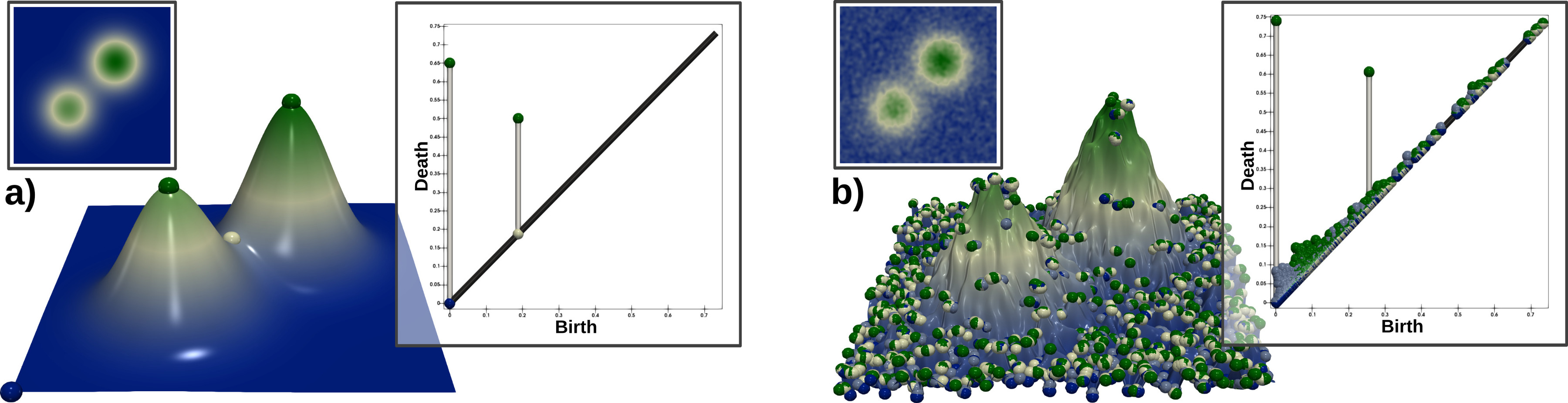
Figure 1: Critical points (spheres, dark blue: minima, dark green: maxima, other: saddles) and persistence diagrams of a clean (a) and noisy (b) 2D scalar field. From left to right: original 2D data, 3D terrain representation, persistence diagram. The diagrams clearly exhibit in both cases two large pairs, corresponding to the main hills. In the noisy diagram (b), small bars near the diagonal correspond to noisy features in the data.

The population of critical points of $f$ can be visually encoded with the notion of persistence diagram [23] (Figure 1). This diagram encodes critical points as pairs $(c,c^{\prime})$ such that $f(c)<f(c^{\prime})$ and $\mathcal{I}(c)=\mathcal{I}(c^{\prime})-1$. These pairs follow the Elder rule [22], which intuitively implies that if two topological features of $f^{-1}_{-\infty}(i)$ meet at a critical point $c^{\prime}$ of $f$, the youngest feature (created at the highest function value) dies, favoring the oldest (created at the lowest function value). In a persistence diagram $\mathcal{D}(f)$, each pair $(c,c^{\prime})$ is represented as a point in 2D at coordinates $\big{(}f(c),f(c^{\prime})\big{)}$, which are the birth and death of the pair respectively. The persistence of the pair is given by its height in the diagram, $P(c,c^{\prime})=|f(c^{\prime})-f(c)|$. It describes the lifespan in the range of the corresponding topological feature. In the following, only the critical point pairs involving local extrema, $(0,1)$ and $\big{(}(d-1),d\big{)}$, will be considered. The consequence of this simplifying assumption are described in section 5. Moreover, for genericity purposes, all persistence evaluations will be normalized with regard to the largest persistence found in the data ($P(c,c^{\prime})\in[0,1]$). In practice, the pairs of the diagram located in the vicinity of the diagonal denote low-amplitude noise while prominent features will be associated with persistent pairs, located far away from the diagonal (Figure 1). The persistence diagram has been extensively studied from a theoretical perspective and its stability to perturbations in the input data has been demonstrated [20]. This stability result greatly motivated the use of persistence in applications, ranging from machine learning [19] to visualization, where it has been shown to significantly help users distinguish salient features from noise.

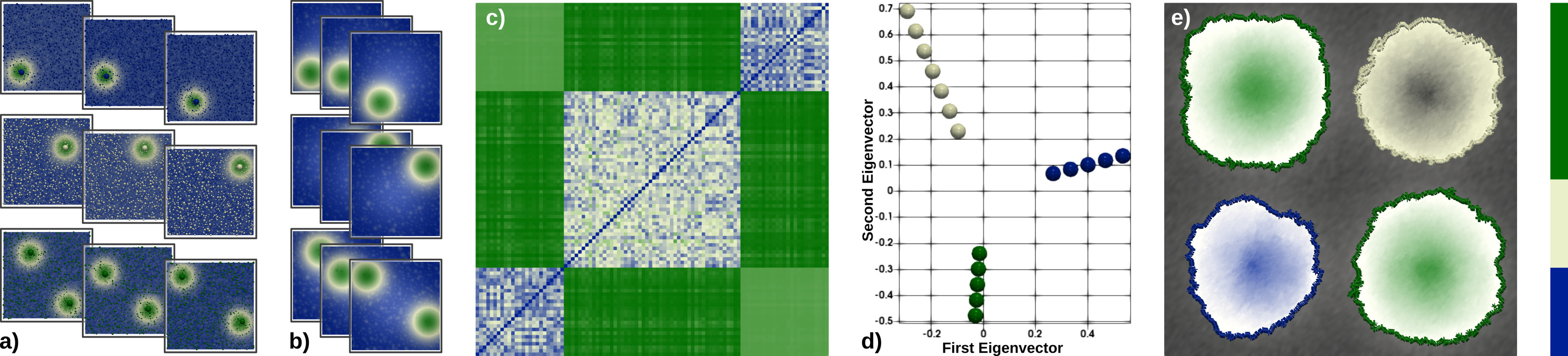
Figure 2: Pipeline overview. (a) Given an ensemble of scalar fields, our approach computes the persistence diagram of each member (critical points are scaled by persistence). (b) To ease the comparison of critical point layouts, each member is transformed into an alternative representation, the persistence map, which denotes the local density in salient features. (c) The distance matrix between the persistence maps is constructed and used to embed each member in a low dimensional feature space, whose first two components can be used to generate planar overviews of the distinct critical point patterns found in the ensemble (d). In this feature space, clusters of members are automatically estimated. (e) The persistence atlas is finally composed by considering the mandatory critical points of each cluster independently (one color per cluster), revealing the main configurations of critical point layouts in the ensemble in terms of numbers and positions. The positional variability of critical points within each mandatory critical point is indicated with a color map. The bar plot (right side) shows the statistics of appearance of each cluster in the ensemble.

1.2 Overview

Our approach is composed of three main steps (Figure 2). It takes as input $n$ PL scalar fields defined on the same PL manifold $\mathcal{M}$.

First (section 2), the persistence map of each ensemble member is computed. The purpose of this representation is to evaluate the spatial distribution of the critical points in each member, while at the same time balancing the contribution of each critical point by its persistence to emphasize salient features and reduce the contribution of noise.

Second (section 3), we leverage spectral embedding to represent each member as a point in a low-dimensional Euclidean space. Distances in this feature space denote dissimilarities between persistence maps. This space is conducive to further statistical analysis of the members which are clustered based on their persistence maps. The first two dimensions of this space are used to generate planar views which enable the direct visualization of the main trends in the ensemble in terms of critical point layouts.

Third (section 4), confidence regions in the geometrical domain are computed for each cluster by leveraging the notion of mandatory critical points [29]. Finally, the confidence regions of all clusters are composed together into the final persistence atlas. This enables the visualization of the regions of occurrence of the most prominent critical points along with estimations of their probability of appearance.

2 Persistence maps

In this section, we introduce the notion of persistence map, a representation of the critical point distribution in each member.

2.1 Motivation

The main target of persistence maps is to facilitate the comparison of two members $f^{(x)}$ and $f^{(y)}$ in terms of the layout of their critical points. As discussed in subsection 0.1, existing topological metrics (e.g. the Bottleneck distance [20]) do not take into account the spatial embedding of the critical points in $\mathcal{M}$ and are therefore not suited for our purpose. Let $C^{(x)}$ and $C^{(y)}$ be the set of critical points of $f^{(x)}$ and $f^{(y)}$ respectively, which can be interpreted as point clouds in $\mathcal{M}$. The problem of comparing the layouts of critical points of $f^{(x)}$ and $f^{(y)}$ then reduces to that of comparing two point clouds, a problem for which no universal solution exists. For instance, the Haussdorff distance, can be seen as a worst-case metric that only measures the distance between the two most distant points of the two sets. This is too limiting for our setting since the similarity of the rest of the point cloud is not assessed. Moreover, due to the presence of noise in the data, it is highly likely in practice that a significant number of the critical points of $f^{(x)}$ and $f^{(y)}$ are noise artifacts. Such artifacts must be taken into account in the similarity estimation in order to reduce their importance and highlight salient features. This last observation is the main motivation behind persistence maps.

A reason for the difficulty in estimating the similarity between the point clouds $C^{(x)}$ and $C^{(y)}$ is that there exists no canonical parameterization of these sets allowing for a straightforward comparison with established distance measures, as can be done for streamlines for instance [26]. $C^{(x)}$ and $C^{(y)}$ may not even be of the same size. This observation motivates the transformation of $C^{(x)}$ and $C^{(y)}$ into an alternate representation that would yield a natural parameterization directly usable with standard distance measures.

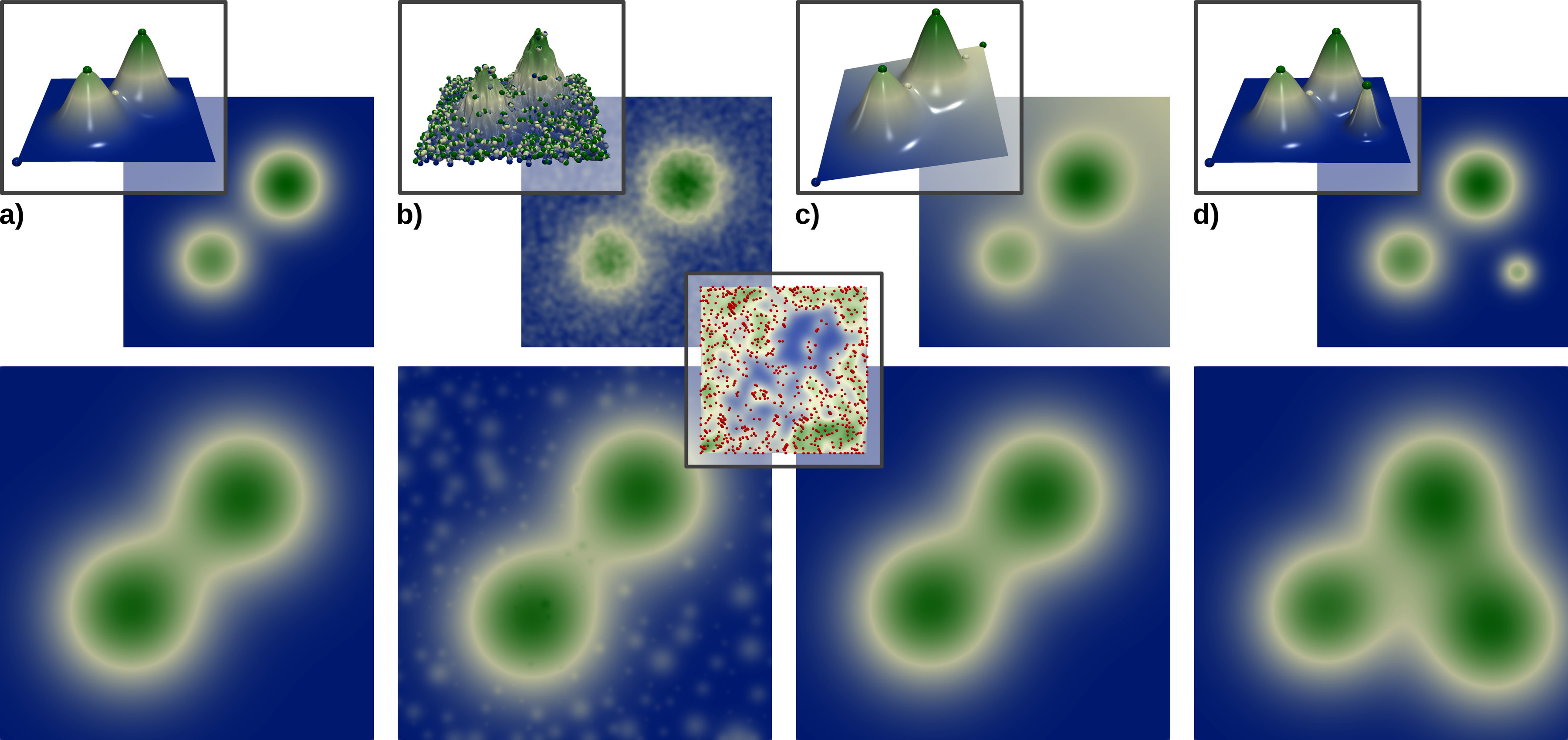
Figure 3: Persistence maps (bottom, maxima only) for four 2D scalar fields (top, inset: terrain view with critical points): $f^{(0)}$ (a), $f^{(1)}$ (b), $f^{(2)}$ (c), $f^{(3)}$ (d). When using constant values for $\alpha(c)$ and $\sigma(c)$, $\phi$ estimates the local density in critical points (b, right inset with maxima in red). In this example, the $L_{2}$ distance separating $f^{(0)}$ from $f^{(1)}$, $f^{(2)}$ and $f^{(3)}$ is $200.79$, $41.03$ and $14.18$ respectively. In contrast, the same distance from $\phi^{(0)}$ to $\phi^{(1)}$, $\phi^{(2)}$ and $\phi^{(3)}$ is $11.09$, $2.84$ and $49.01$ respectively. This different ordering indicates that the $L_{2}$ distance between persistence maps is less sensitive to noise and global shifts in data values and better discriminates changes in salient features.

2.2 Formulation

Breckner and Möller [16] faced a similar problem in the context of isosurface comparison and introduced a signed distance field transform, measuring the distance between each vertex of $\mathcal{M}$ and the considered isosurface. Then, the similarity between two isosurfaces can be evaluated based on the standard $L_{2}$ distance between their distance transforms. The same idea has been later used by Ferstl et al. [27] in a context that resembles our setting (isocontour clustering for level set variability analysis and visualization). We build upon this strategy to construct persistence maps. In particular, one could derive a distance transform for a critical point set $C$, by considering for each vertex $v\in\mathcal{M}$, the distance to the closest critical point of $C$. However, such a distance transform would be highly sensitive to the presence of noise in the data since all the critical points of $f$ would be considered for its computation. Therefore, it is necessary to develop a transformation where the contribution of each critical point could be weighted by an importance measure, such as topological persistence [23]. While such a weighting strategy is difficult to elaborate for distance fields, it is much easier to derive for sums of gaussian radial basis functions. In particular, let $\phi:\mathcal{M}\rightarrow\mathbb{R}^{+}$ be the following scalar function, where $\alpha(c)$ and $\sigma(c)$ are scalars controlling the amplitude and spatial spread of the contribution of the critical point $c$:

$$\vspace{-1ex}\phi(v)=\sum_{c\in C}\alpha(c)e^{-{{||v-c||_{2}^{2}}\over{2\sigma(c)^{2}}}}\vspace{-1ex}$$ (1)

If constant values are considered for both $\alpha(c)$ and $\sigma(c)$, $\phi$ is a measure of the local critical point density (Figure 3, inset). To limit the importance of noisy critical points in this density estimation and to highlight salient features, we use persistence as an importance measure in the expressions of $\alpha(c)$ and $\sigma(c)$ as follows, where $P(c)$ stands for the persistence of the critical point pair containing $c$ in $\mathcal{D}(f)$:

$$\vspace{-1ex}\alpha(c)=P(c),\quad\sigma(c)=\gamma P(c)\vspace{-1ex}$$ (2)

$\gamma$ controls the focus that is given to salient features in terms of their spread in the spatial domain. Distances are normalized with regard to the bounding box diagonal. We have found that $\gamma=0.1$ is a good value in practice. This representation resembles the notion of persistence images [3], which focuses on range rather than domain density.

2.3 Distances

Since they are both defined on the same spatial domain $\mathcal{M}$, the persistence maps $\phi^{(x)}$ and $\phi^{(y)}$ of two critical points sets $C^{(x)}$ and $C^{(y)}$ benefit from a common parameterization and their distance can be estimated with standard distance measures, such as the $L_{2}$ norm:

$$\vspace{-1ex}||\phi^{(x)}-\phi^{(y)}||_{2}=\sqrt{\sum_{v\in\mathcal{M}}\big{(}\phi^{(x)}(v)-\phi^{(y)}(v)\big{)}^{2}}\vspace{-1ex}$$ (3)

By design, this metric is robust to noise, since the contribution of critical points to the persistence maps is weighted by their persistence (Eq. 2). Hence, small persistence pairs (typically corresponding to low amplitude noise, Figure 1(b)) will have a negligible contribution in practice to the persistence maps (Figure 3(b), further discussion in subsection 5.4). This is important since small scale additive noise often occur in practice even for assumed smooth simulation data. This metric is also robust by design to global variations in data values which do not change the critical point spatial layout, since the actual data values are not taken into account in the persistence map. In contrast, the standard $L_{2}$ distance $||f^{(x)}-f^{(y)}||_{2}$ would tend to miss the possible preservation of salient features in the presence of global shifts in data values, as can be the case with seasonal effects in climate data. Finally, the distance $||\phi^{(x)}-\phi^{(y)}||_{2}$ is specifically designed to penalize changes in the layout of salient critical points. The above properties are illustrated in Figure 3, which shows persistence maps on a toy example, $f^{(0)}$, along with three variants: $f^{(1)}$ with additive noise, $f^{(2)}$ which contains a global shift in data values (slope), and $f^{(3)}$ which contains an additional salient feature. For this data, we have: $||f^{(0)}-f^{(3)}||_{2}<||f^{(0)}-f^{(2)}||_{2}<||f^{(0)}-f^{(1)}||_{2}$. In other words, with the $L_{2}$ distance between the actual data values, the noise affected dataset ($f^{(1)}$) is the most distant to the original ($f^{(0)}$), while the dataset with a drastic change in critical point layout ($f^{(3)}$) is the closest. In contrast, the $L_{2}$ distance between the corresponding persistence maps results in a different ordering: $||\phi^{(0)}-\phi^{(2)}||_{2}<||\phi^{(0)}-\phi^{(1)}||_{2}<||\phi^{(0)}-\phi^{(3)}||_{2}$. In other words, with the persistence map metric, the closest data set from the original ($f^{(0)}$) is the one which better preserves the critical point layout ($f^{(2)}$), while the most distant is the one which changes it the most ($f^{(3)}$). This indicates that the metric $||\phi^{(x)}-\phi^{(y)}||_{2}$ is indeed more robust to noise and global shift in data values than $||f^{(x)}-f^{(y)}||_{2}$ and that it better describes variations in the layout of salient critical points. Our distance (Eq. 3) resembles the kernel distance defined for generic point cloud data [61]. In contrast, persistence maps focus on the critical points of a scalar field (instead of generic point clouds). This allows to additionally consider in the density estimation the persistence of each critical point as an importance measure (Eq. 2), to highlight salient features and reduce the effect of noise.

3 Space of persistence maps

As described above, the $L_{2}$ distance between persistence maps is a good candidate to compare the spatial layout of critical points between two members. Based on this metric, a distance matrix $\Phi$ is computed for the entire ensemble, with $\Phi_{xy}=||\phi^{(x)}-\phi^{(y)}||_{2}$, and then normalized. In this section, we exploit this distance matrix to visualize and identify the main trends in critical point layouts within the ensemble.

3.1 Low dimensional embedding

To directly visualize the global trends in critical point layouts, we first consider a low dimensional embedding of the ensemble into a space of persistence maps, noted $\mathcal{P}$, where each map $\phi$ is represented by a point and where distances between points denote distances between persistence maps. For this, we employ established methods for non-linear dimensionality reduction [87, 13]. In particular, we focus on the spectral approach by Belkin et al. [9] based on Laplacian eigenmaps, which has been shown to better preserve locality than standard methods such as principal component analysis [2] or Isomap [81]. This property is particularly beneficial if clustering is subsequently considered, which is the case in our framework (subsection 3.2). For completeness, we briefly sketch the main steps of the Laplacian eigenmap approach and we refer the reader to [9] for further details.

First, an adjacency graph is constructed, where the $x^{th}$ node represents the $x^{th}$ ensemble member and where arcs are introduced between the node $x$ and its $n_{n}$ nearest neighbors (according to the distance matrix $\Phi$). In practice, we set $n_{n}$ to a default recommended value ($5$). Next, a weight matrix $W$ is constructed such that $W_{xy}=1$ if $x$ and $y$ are connected in the adjacency graph and $0$ otherwise. A diagonal matrix $D$ is also established such that $D_{xx}=\sum_{y}W_{xy}$. Then, the Laplacian, $L$, of the adjacency graph is considered as $L=D-W$, which is a symmetric, positive semidefinite $n\times n$ matrix [9]. Finally, the low-dimensonal space $\mathcal{P}$ is constructed by projecting each ensemble member along the $n_{d}$ first eigenvectors $\psi\in\mathbb{R}^{n}\times\mathbb{R}^{n}$ of $L$, which are solutions of the generalized eigenvector problem: $L\psi=\lambda D\psi$ (where $\lambda\in\mathbb{R}^{n}$ stands for the $n$ eigenvalues of $L$). In practice, the first eigenvector $\psi_{0}$ is discarded, as suggested by Belkin et al. [9]. Thus, the $x^{th}$ ensemble member is then embedded at position $\psi^{(x)}=\big{(}\psi_{1}(x),\dots,\psi_{n_{d}}(x)\big{)}$. Since the first eigenvectors of $L$ are usually considered to be the most informative [85], for visualization purpose, we typically represent planar layouts of the space of persistence maps $\mathcal{P}$ by only considering the first two components of this vector ($\psi_{1}(x),\psi_{2}(x)$).

3.2 Persistence map clusters

Figure 2(d) shows a typical 2D layout of the first two dimensions of the space of persistence maps, $\mathcal{P}$, for a toy ensemble dataset. As shown in this example, clear patterns that correspond to distinct trends in critical point layout emerge from this visualization. To quantitatively analyze these patterns, we next employ clustering algorithms. In particular, we employ the popular $k$-means algorithm [45], which has been shown to be well suited for a combined usage with spectral emdedding (subsection 3.1), yiedling the notion of spectral clustering [77]. This algorithm is based on the classical Lloyd relaxation scheme [43] which, given an initial assignment of $k$ cluster centroids chosen among the data points, assigns each data point to the cluster of its closest centroid. Next, for each cluster, a new centroid is selected as the point being the closest to the new cluster barycenter and the procedure is iterated until convergence. Note that for the above clustering procedure, the spectral clustering literature recommends to only use the $k$ first components of $\psi^{(x)}$ [85], although we found in practice that with our implementation, the most stable results were obtained for $n_{d}=k-1$.

The number $k$ of clusters to be considered is particularly important as it directly corresponds to the number of trends which can be visualized in the ensemble. While we offer users the possibility to explicitly specify pre-defined values of $k$, we also provide an automatic estimation procedure. Several statistical measures have been studied for the automatic estimation of $k$, such as the Bayesian Information Criterion [55]. In the specific case of spectral clustering however, it has been shown that the eigenvalues of the Laplacian matrix (subsection 3.1) already exhibit important hints regarding cluster numbers and that they are particularly useful to identify proper values for $k$. In particular, the first eigenvalue $\lambda_{k}$ resulting in a significant eigengap $\delta_{k}=|\lambda_{k}-\lambda_{k+1}|$ is usually considered as a good value for $k$ (see von Luxburg [85] for formal arguments based on perturbation theory). Thus, in practice, we provide as an initial guess for $k$, the position of the first local maximum of eigengap $\delta_{k}$. Figure 4 plots the evolution of the eigengaps for the example of Figure 2. As shown in this figure, the appropriate number of clusters for this specific dataset indeed corresponds to the first local maximum of eigengap ($k=3$). Note that several other local maxima of eigengaps occur for higher eigenvalues. We also offer users the possibility to interactively explore them individually.

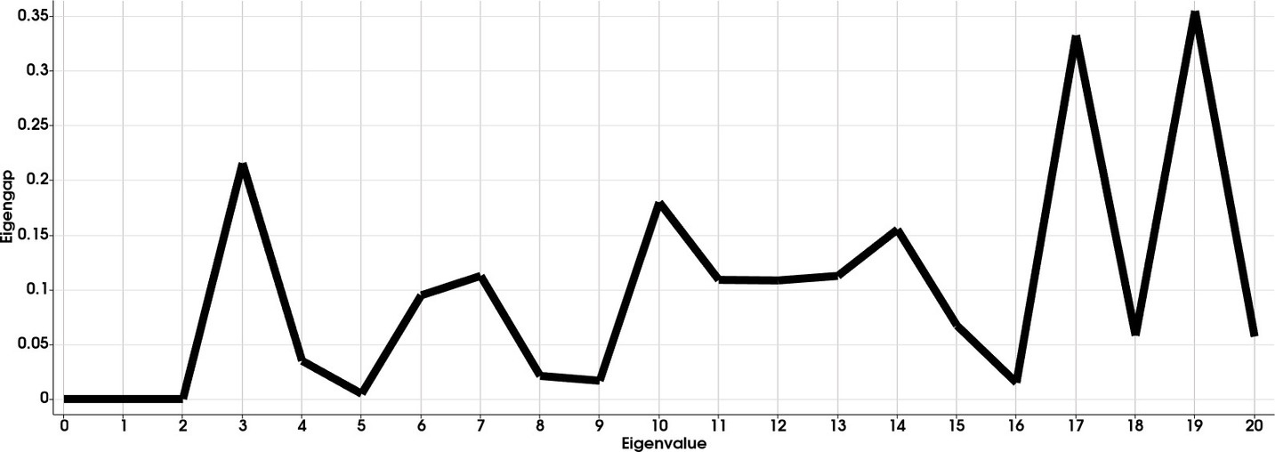
Figure 4: Eigengaps computed for the example shown in Figure 2. Our approach uses the position of the first local maximum of eigengap as an initial value for the number of clusters $k$. Our framework also offers the possibility to explore the other maxima, as well as arbitrary $k$ values.

4 Confidence regions for persistence map clusters

The major trends in critical point layout in the ensemble can be identified by clustering the persistence maps (section 3). In this section, we describe how to visualize the spatial variability of critical points within each of the identified clusters.

4.1 Per cluster variability analysis

The clustering procedure described in the previous section identifies disjoints subsets of ensemble members which share a common pattern in critical point layout. Let $f^{(X)}=\{f^{(x_{0})},f^{(x_{1})},\dots f^{(x_{m})}\}$ be such a subset ($m<n$). To understand the variability of critical points within this subset, one needs first (i) to identify a common topological structure among all of the members of $f^{(X)}$ and second (ii) to analyze its spatial variability. As discussed in subsection 0.1, several approaches have been proposed to study the positional uncertainty of critical points. Among those, we focus on the approach based on mandatory critical points [29] since it is based on point-wise intervals and is, therefore, well suited for the analysis of ensemble data, where no specific assumption can be made about the structure of the point-wise random variables locally modeling the data variability. For completeness, we briefly sketch the main steps of this method and refer the reader to [29] for further details.

First, pointwise scalar value bounds are extracted as two scalar fields $f^{-}:\mathcal{M}\rightarrow\mathbb{R}$ and $f^{+}:\mathcal{M}\rightarrow\mathbb{R}$, such that $f^{-}(v)=\min_{f^{(x)}\in f^{(X)}}f^{(x)}(v)$ and $f^{+}(v)=\max_{f^{(x)}\in f^{(X)}}f^{(x)}(v)$. Given an isovalue $i$, let $C^{-}(i)$ be a connected component of sub-level set of $f^{-}$ (blue region in Figure 5). By construction, for each vertex $v$ in $C^{-}(i)$, there exists at least one member $f^{(x)}\in f^{(X)}$ for which $f^{(x)}(v)\leq i$. Then, there exists a member $f^{(x)}$ for which a connected component of sub-level set $C^{(x)}$ passes through $v$ at isovalue $i$ (gray regions in Figure 5). Then, $C^{-}(i)$ is called a candidate region for the appearance of a local minimum (responsible for the creation of the component $C^{(x)}$ in $f^{(x)}$).

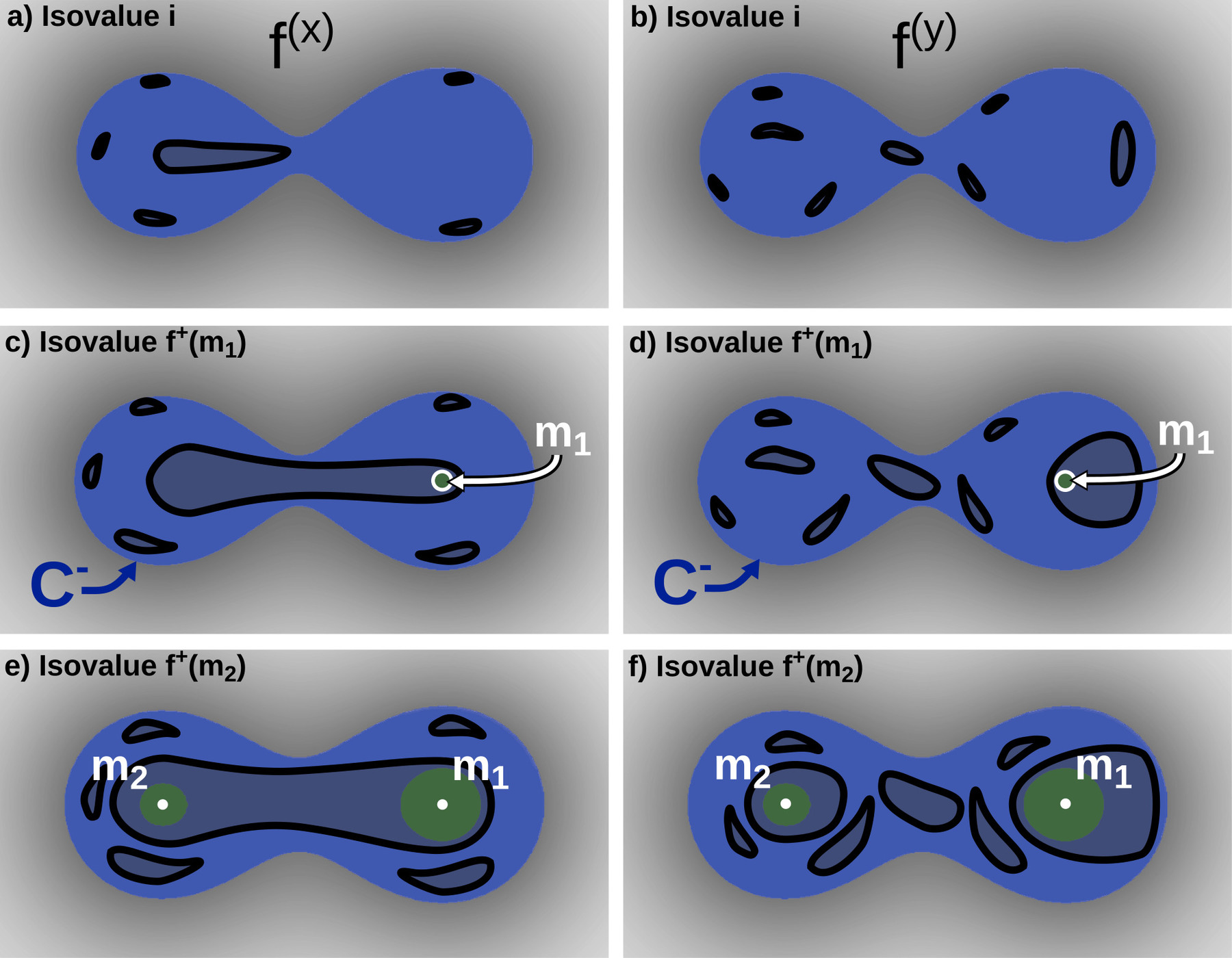
Figure 5: Sub-level sets of $f^{-}$ (blue) and $f^{+}$ (green) at three different isovalues $i<f^{+}(m_{1})<f^{+}(m_{2})$ with $m_{1}$ and $m_{2}$ being minima of $f^{+}$. The sub-level set components $C^{(x)}$ and $C^{(y)}$ of two ensemble members $f^{(x)}$ (left) and $f^{(y)}$ (right) are shown in gray.

Let $m_{1}$ be a minimum of $f^{+}$. Since $f^{-}$ and $f^{+}$ are nested, $m_{1}$ must be located inside a connected component of sub-level set of $f^{-}$ at isovalue $f^{+}(m_{1})$. Let $C^{-}\big{(}f^{+}(m_{1})\big{)}$ be that region and let us first consider that $m_{1}$ is the only minimum of $f^{+}$ in it. At isovalue $f^{+}(m_{1})$, by construction, all the members $f^{(x)}\in f^{(X)}$ are such that $f^{(x)}(m_{1})\leq f^{+}(m_{1})$. This means, that for all the members $f^{(x)}$ of the subset $f^{(X)}$, there exists a connected component of sub-level set $C^{(x)}$ passing through $m_{1}$ (gray components containing $m_{1}$ in Figure 5(c) and Figure 5(d)). In particular, this connected component was created at an earlier isovalue, at one of the vertices of the corresponding candidate region, $C^{-}\big{(}f^{+}(m_{1})\big{)}$. Overall, this means that $C^{-}\big{(}f^{+}(m_{1})\big{)}$ must contain at least one minimum (responsible for the initial creation of the component $C^{(x)}$) for all the members of $f^{(X)}$. Thus, the region $C^{-}\big{(}f^{+}(m_{1})\big{)}$ is called a mandatory minimum: a minimal connected component $C^{-}$ of $\mathcal{M}$, associated with a minimal interval $I^{-}=[min_{v\in C^{-}}f^{-}(v),min_{v\in C^{-}}f^{+}(v)]$, such that any $f^{(x)}$ contains at least one minimum $m_{1}$ in $C^{-}$ with $f^{(x)}(m_{1})\in I^{-}$.

Figure 5 illustrates this process where candidate regions (blue) may contain several connected components $C^{(x)}$ (gray) of sub-level set of ensemble members ($m_{1}$ is shown in green). Note that if the candidate region contains a second minimum $m_{2}$ such that $f^{+}(m_{1})<f^{+}(m_{2})$, this implies that the sub-level set of all members pass through $m_{2}$ as well. However, they may do so with the component $C^{(x)}$ which already contains $m_{1}$ (Figure 5(e)). Thus, the existence of such a second minimum $m_{2}$ does not necessarily imply the existence of an additional minimum in $f^{(x)}$, as it is the case in Figure 5(e) (as opposed to Figure 5(f)). As discussed in section 5, this observation may have important practical implications, as it may prevent the detection of a mandatory critical point in case of high pointwise value variability $|f^{+}(v)-f^{-}(v)|$.

Other types of mandatory critical points are extracted similarly, as described in [29]. Eventually, each cluster $f^{(X)}$ is associated with a collection of mandatory critical points, which describe the spatial variability of the common topological structure found among its members.

4.2 Global visualization

The mandatory critical points can be visualized for each cluster independently, by displaying each critical component with a colored region. Additionally, the positional variability of critical points within each region can be estimated and visualized as follows. Given a histogram representation of the data values taken by a vertex $v$ in $f^{(X)}$, we estimate this variability as the probability of $v$ to admit a scalar value within the critical interval of each mandatory critical point. Finally, we estimate the overall probability of appearance of a mandatory critical point as the proportion between the size of $f^{(X)}$ and the total number, $n$, of members in the ensemble. As shown in Figure 2 (right), this probability can be visualized in the form of a barplot. The Persistence Atlas is then created from a collection of confidence maps (composed together) that provide for each major trend found in the ensemble, confidence regions for the appearance of critical points along with their probability of appearance, as well as, their individual critical point spatial variability given by the above estimation (Figure 2).

5 Results

This section presents experimental results obtained on a desktop computer with a Xeon CPU (2.6 GHz, 2x6 cores), with 64 GB of RAM. For the computation of the persistence diagrams, we used the Topology ToolKit (TTK) [83]. For the spectral embedding and clustering, we adapted classes from the scikit-learn package [54]. The other components of our approach have been implemented as TTK modules.

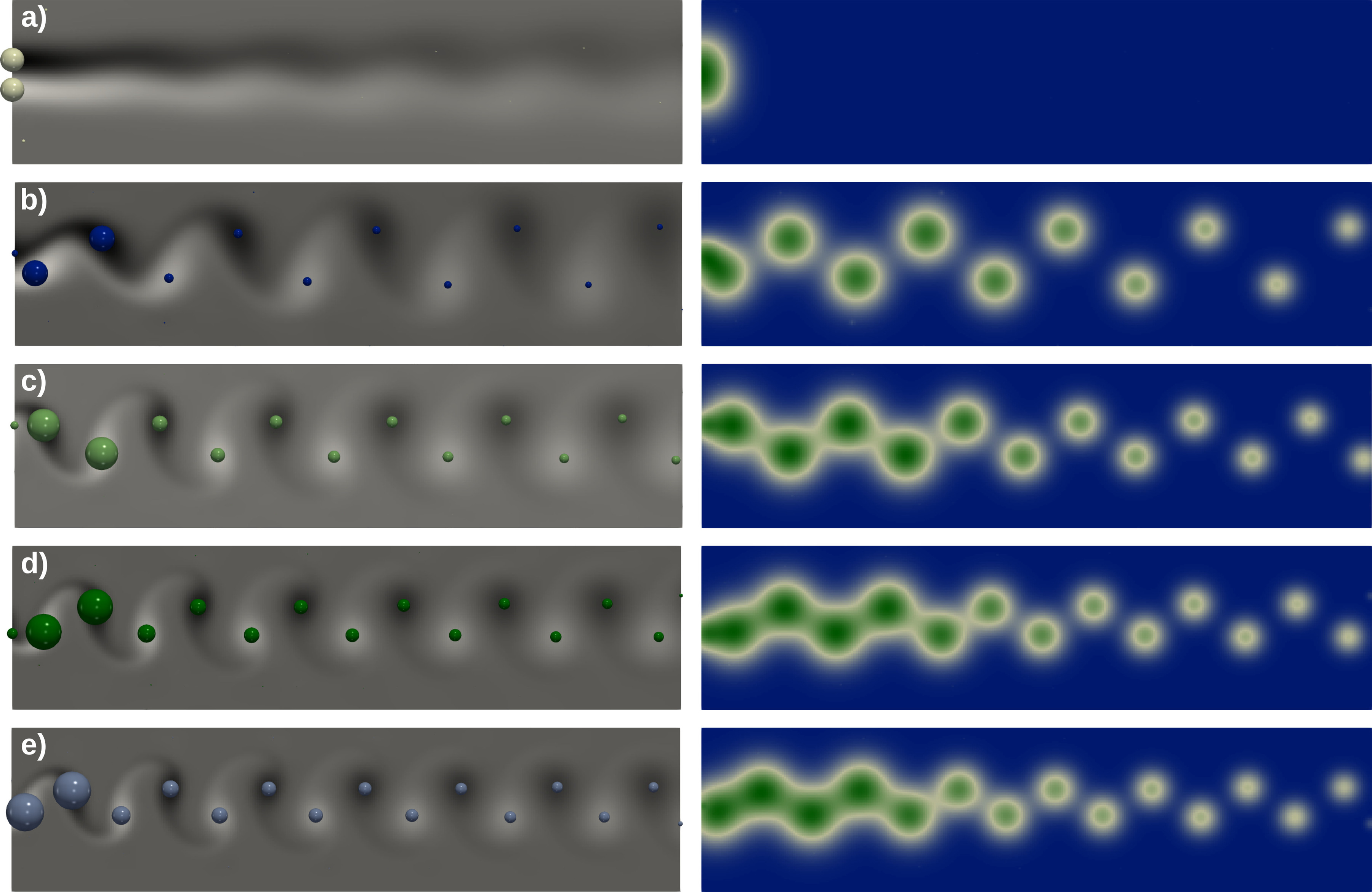
Figure 6: Five representative members of the ensemble of Persistence Atlas for Critical Point Variability in Ensembles. Critical points (minima and maxima) are shown with spheres scaled by their persistence (left). Persistence maps are shown on the right.

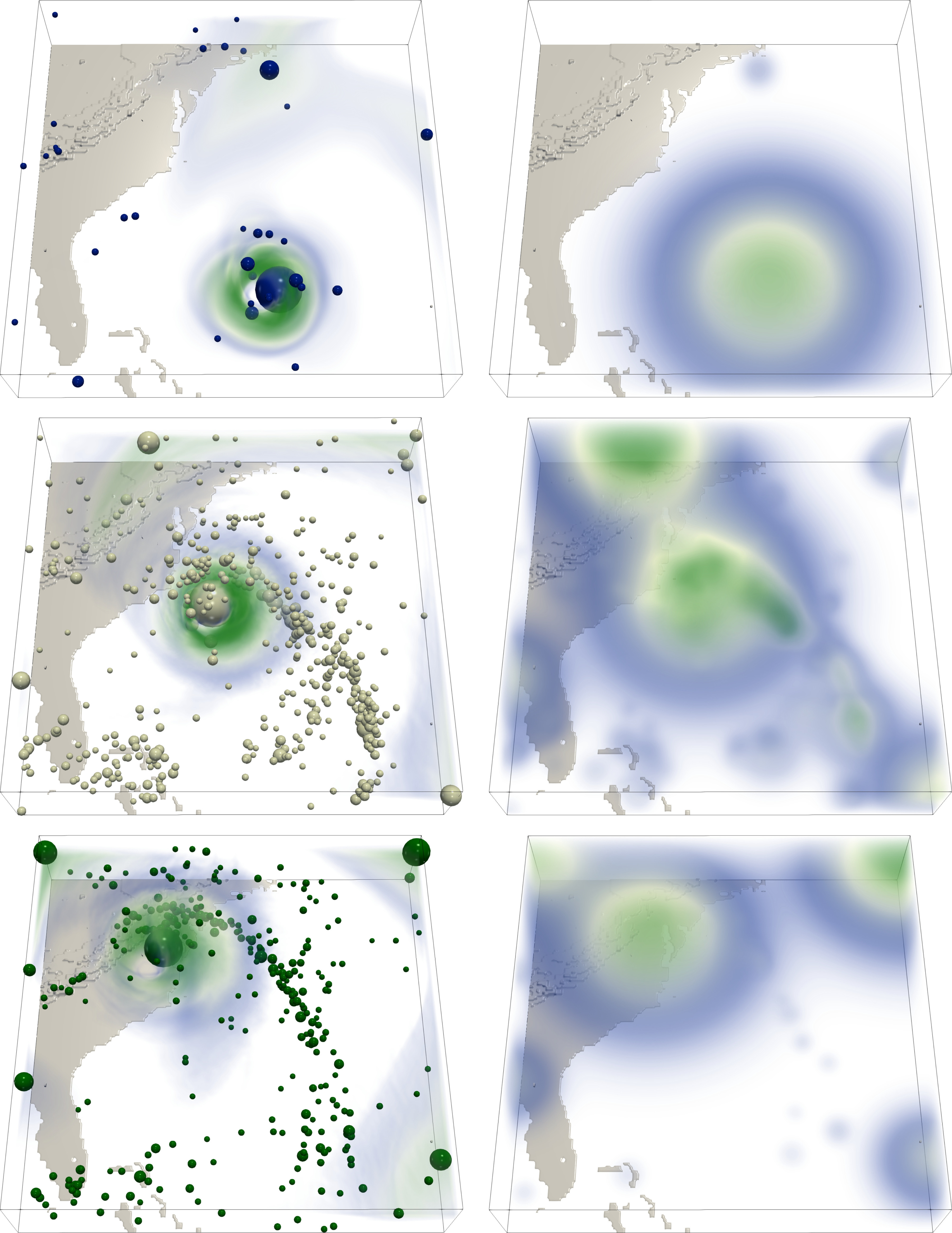
Figure 7: Three representative members for the Isabel volumetric ensemble (left). Local maxima (scaled by persistence) of velocity magnitude capture the eyewall of the hurricane, high wind speed peripheral regions as well as the hurricane’s tail (second and third row). The persistence maps (local maxima only, right) capture these subtle features by construction, while taking less into account noisy critical points (smallest spheres).

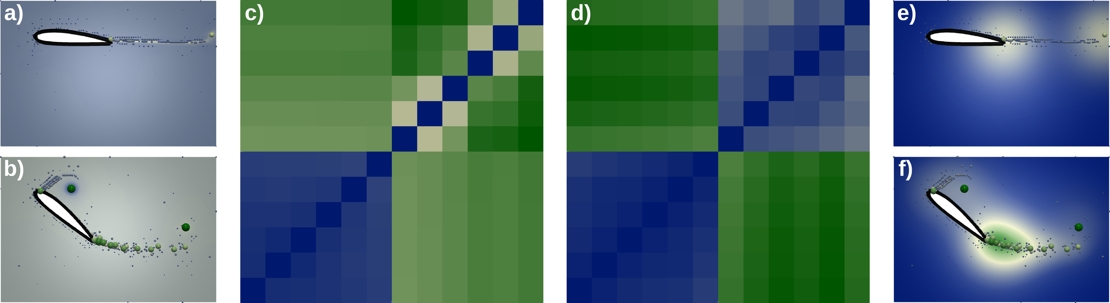
Figure 8: Two representative members of the Starting vortex ensemble ((a) and (b)) along with their critical points scaled by persistence. Given the small spatial extent of these features, the $L_{2}$ norm between the actual data values fails at capturing similarities between members belonging to the bottom configuration (b), as denoted by the corresponding distance matrix (c), where distances are important (green) in the upper-right corner. In contrast, the distance matrix (d) computed from persistence maps ((e) and (f)) exhibits much smaller distances (blue) between these members, facilitating their gathering in the low dimensional space $\mathcal{P}$.

Table 1: Running time (in seconds, with 12 cores) for the different steps of our approach: persistence maps ($P.M.$, subsection 2.2), distance matrix ($D.M.$, subsection 2.3), low-dimensional embedding ($E.$, subsection 3.1), clustering ($C.$, subsection 3.2) and mandatory critical points ($M.C.P.$, section 4).

Dataset	$n$	$|\mathcal{M}^{0}|$	P.M.	D.M.	E.	C.	M.C.P.	Total
Gaussians (Figure 2)	100	262,144	57.28	1.03	0.67	0.08	2.53	61.59
Vortex street (Persistence Atlas for Critical Point Variability in Ensembles)	45	30,000	2.28	0.02	0.67	0.09	0.22	3.28
Starting vortex (Figure 9)	12	1,500,000	61.44	0.09	0.65	0.07	9.08	71.33
Isabel (Figure 10)	12	3,125,000	168.70	0.18	0.63	0.07	41.84	211.68
Sea Surface Height (Figure 11)	48	1,036,800	290.25	0.99	0.65	0.08	8.38	300.35

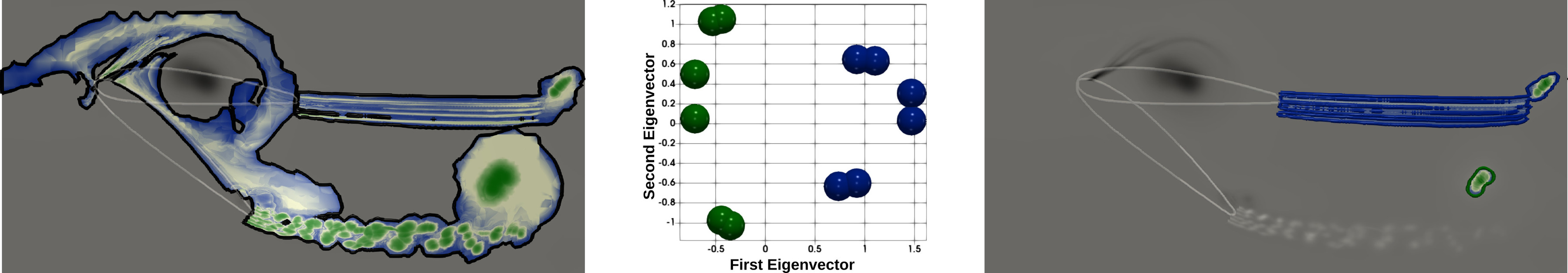
Figure 9: Mandatory critical point for the entire Starting vortex ensemble (left) and the corresponding critical point positional variability estimation (color map, left). Given the trend variability of this ensemble, this global extraction identifies only one, very large, mandatory maximum (colored region) describing both regimes, although these two vortices never occur simultaneously in the data. The persistence atlas automatically identifies the two trends present in the data, as shown in the planar view (center), resulting in much more accurate predictions for the appearance of the distinctly identified vortices (green and blue regions, right).

Figure 10: Mandatory critical point for the Isabel ensemble, viewed from above and below (a). Given the trend variability of this ensemble, this extraction identifies only one, very large, mandatory maximum (region colored by critical point positional variability) merging the three distinct states of the hurricane (formation, drift and landfall). In contrast, the persistence atlas manages to isolate these three states and provides more accurate confidence regions for the position of the hurricane eyewall (colored regions).

5.1 Experiments

Figures Persistence Atlas for Critical Point Variability in Ensembles and 6 to 11 report various experiments on simulated and acquired 2D and 3D ensemble datasets. Persistence Atlas for Critical Point Variability in Ensembles presents our entire approach on an ensemble of 45 von Kármán vortex streets, where the considered scalar data is the orthogonal component of the curl taken at a fixed time-step, for five different fluids of distinct viscosity (9 runs per fluid, each run with varying Reynolds numbers). For such scalar fields, local extrema are typically considered as reliable estimations of the center of the vortices. Extrema of a few representative members (Persistence Atlas for Critical Point Variability in Ensembles(a)) exhibit clearly distinct layout patterns, in terms of both the position and number of vortices, revealing high spatial and trend variabilities within the ensemble. The mandatory critical points estimated for the entire ensemble are particularly conservative given these variabilities: only one region is extracted for each side of the street (one for minima, one for maxima). The persistence atlas manages to automatically identify five clusters in the ensemble, corresponding to distinct critical point layouts (one per viscosity regime). The mandatory critical points extracted from these clusters provide more accurate and useful predictions for the appearance of vortices (colored regions in (d) to (h), one color per cluster). In particular, the persistence atlas reveals that the number of vortices increases with the Reynolds numbers (from left to right: 6, 10, 12, 14 and 15 vortices) while the spatial variability of each vortex tends to decrease for increasing Reynolds numbers (smaller mandatory critical points). Figure 6 illustrates persistence maps for five representative members of the ensemble and shows how salient features are captured by this representation. Figure 7 shows persistence maps on a volumetric ensemble composed of groups of key timesteps (formation, drift and landfall) in the simulation of the Isabel hurricane [76]. For such datasets, the eyewall of the hurricane is typically characterized by high wind velocities (green regions, Figure 7, left) and contains salient maxima. In particular, this figure shows that subtle features of the hurricane (eyewall, high wind speed peripheral regions and hurricane’s tail) are well captured by local maxima of the wind velocity magnitude and by the corresponding persistence maps. As discussed in subsection 2.3, the $L_{2}$ norm between persistence maps is more suited to our purpose than the $L_{2}$ norm between the actual data values, since it is more robust to noise and global shifts in data values, while better discriminating changes in salient features (Figure 3). Figure 8 further exemplifies this observation on the Starting vortex ensemble, which includes 12 runs of a 2D simulation of the formation of a vortex behind a wing, for two distinct wing configurations. The considered scalar field is the curl orthogonal component and salient extrema are expected at the center of vortices. Given the small spatial extent of the features behind the wing, the $L_{2}$ norm between the actual data values fails at capturing similarities between members belonging to the second configuration, as denoted by the corresponding distance matrix, where distances are important in the upper-right corner. In particular, two members belonging to the same wing configuration are reported by this distance as the two furthest members (darkest green entry). In contrast, the distance matrix computed from persistence maps exhibits much smaller (resp. higher) distances between the members belonging to a common (resp. distinct) wing configuration.

Figure 9 shows the persistence atlas for the Starting vortex ensemble. Given the trend variability of this dataset, the mandatory critical points computed from the entire ensemble exhibit only one, very large, mandatory maximum (colored region) describing the appareance of vortices for both wing configurations, although these two vortices never occur simultaneously in the data. The persistence atlas automatically identifies the two trends present in the data, as shown in the planar view (center), resulting in much more accurate predictions for the appearance of the distinctly identified vortices (green and blue region, right). Figure 10 shows the persistence atlas for the Isabel ensemble. Similarly to the previous example, mandatory critical points computed from the entire ensemble identify only one, very large, mandatory maximum, which merges the three distinct states of the hurricane. In contrast, the persistence atlas manages to isolate these three states and provides much more accurate confidence regions for the position of the hurricane eyewall. Note that this example is the only dataset for which the initial automatic suggestion for the number of clusters $k$ provided by the eigengap heuristic needed adjustment. All the other results have been generated with the automatic suggestion. Figure 11 shows the persistence atlas for the Sea surface height ensemble, which is composed of 48 observations taken in January, April, July and October 2012 (https://ecco.jpl.nasa.gov/products/all/). For such datasets, salient extrema in the height are expected at the center of eddies. The mandatory critical points globally extracted on the entire ensemble identify only few features (Figure 11(a)), due to the high pointwise data variability (subsection 4.1). The clustering automatically performed by our approach based on the persistence maps correctly identifies four clusters, corresponding to the four seasons: winter (c), spring (d), summer (e) and fall (f). This seasonal decomposition drastically reduces pointwise data variability and enables mandatory critical points to identify many more structures, corresponding to clockwise and counterwise vortices (minima and maxima) and revealing complex structures in the Gulf stream area (insets). Note that, for this example, due to the high number of critical points and their respective proximity, the parameter $\gamma$, controlling the spread of salient features in the persistence map, has been set to $0.01$ instead of the default value ($0.1$).

5.2 Time performance

Table 1 presents the running times we obtained for the datasets presented in this paper. The most time consuming portion of our approach is the computation of the persistence maps, which typically needs to be run for each ensemble member as a pre-process. Since the number of pairs in the diagram is typically proportional to the number $|\mathcal{M}^{0}|$ of vertices in the domain, this part requires $O(n\times|\mathcal{M}^{0}|^{2})$ steps overall. In practice, to accelerate this computation, we ignore all pairs with a persistence less than $1\%$ of the total function range. The distance matrix computation takes $O(n^{2}\times|\mathcal{M}^{0}|)$ steps, but since $n$ is typically much smaller than $|\mathcal{M}^{0}|$, the computation time for this step is small in practice. Both the spectral embedding (subsection 3.1) and clustering (subsection 3.2) employ iterative solvers but these computations are typically the fastest steps of the pipeline. The computation of the mandatory critical points for each cluster admits quadratic complexity $O(|\mathcal{M}^{0}|^{2})$.

Most of these steps can be trivially parallelized. The persistence diagram is computed in parallel [30] and the persistence map can be evaluated independently for each vertex. Each entry of the distance matrix $\Phi$ (subsection 2.3) can be computed independently. Finally, mandatory critical points are computed in parallel for each cluster. As reported in Table 1, once the persistence maps have been computed in a pre-process, the rest of the framework is sufficiently fast to allow interactivity.

5.3 Comparison

In this section, we compare our approach to alternative critical point clustering strategies. First, we consider a baseline approach, which consists in simply clustering persistent critical points in the spatial domain, by using a vanilla implementation of spectral clustering, combined with our eigengap heuristic for the automatic suggestion of the number of clusters (subsection 3.2). Once such clusters have been computed, this baseline strategy evaluates confidence regions for the appearance of critical points by considering the convex hull of each cluster in the spatial domain. As shown in Figure 12(a), this simple strategy provides unsatisfactory results for the von Kármán vortex street ensemble (Persistence Atlas for Critical Point Variability in Ensembles) since features which never occur simultaneously in the ensemble are clustered based on their proximity. In particular, the extracted clusters mix the two types of vortices (right and left) and group them based on their distance from the obstacle (bottom).

To further evaluate our approach, we consider the ensemble from Figure 2, which we split in half into a training and test ensemble. The training ensemble is analyzed with (i) the baseline approach (Figure 12(b)), (ii) a strategy based on the kernel method by Reininghaus et al. [70] (Figure 12(c), where the distance matrix considered for clustering has been generated with the authors’ implementation of the kernel method [40] run with default parameters) and (iii) the persistence atlas (Figure 12(e)). To quantitatively evaluate the prediction performance of these approaches, we consider the persistent critical points of the test ensemble having a persistence higher than 20% of the function range. Next, the test critical points are assigned to the confidence region in which they land in the domain (spheres of matching colors in Figure 12). As shown in Figure 12(b), the baseline approach overestimates the number of clusters. In particular, it fails at clustering together features which always occur simultaneously (dark green and light blue clusters in Figure 12(b)). Kernel based methods for persistence diagrams [70, 40] do not take the spatial embedding of critical points into account (Figure 12(c)) and cluster members with the same persistence profile, irrespective of the features’ location. This leads to an underestimated number of clusters: the blue and white clusters of Figure 2, which both include a single very persistent maximum, are erroneously merged although the corresponding features never occur simultaneously in the ensemble. Moreover, convex hulls obtained from this clustering overestimate the size of the confidence regions in the presence of multiple salient features per cluster. Even when the correct clustering is explicitly provided (Figure 12(d)), confidence regions based on convex hulls miss 21% of the persistent critical points of the test ensemble. In contrast, the persistence atlas (Figure 12(e)) provides a correct prediction for 100% of the critical points of the test ensemble, which illustrates the quantitative performance of the persistence atlas regarding critical point prediction.

Figure 11: Persistence atlas for the Sea surface height ensemble. (a) Mandatory critical points for the entire ensemble miss many features and over-estimate the spatial variability of the extracted structures. (b) The planar layout of the space of persistence maps shows the automatically evaluated clustering of the ensemble (one color per cluster), which correspond to the four seasons. (c), (d), (e) and (f) The mandatory critical points for each of the identified clusters (respectively: winter, spring, summer and fall) provide a more precise critical point variability estimation, revealing hundreds of vortices (blue: minima, green: maxima).

5.4 Limitations

Our entire pipeline assumes that the input data is given as a collection of piecewise linear scalar fields (subsection 1.1). In many applications [74], this may be too restrictive (motivating taylored interpolants for uncertainty modeling [75]). However, generalizing the TDA arsenal to a larger set of interpolants is a vast research topic (see [49] for an example) which goes beyond the scope of this paper. Our approach focuses on $(0,1)$ and $\big{(}(d-1),d\big{)})$ persistence pairs, which correspond to pairs only involving minima and maxima. Persistence maps (Eq. 1) are therefore only computed based on the location of either the minima or maxima (Figs. 2, 9 and 7), or both (Figs. 6 and 11). Hence, saddle points are not taken into account by our framework in its current form. However, we have found that in practice the correspondence between saddle points and features of interest was less clear in our applications. Also, when the data exhibits salient large flat plateaus, persistent critical points can appear in arbitrary locations inside these plateaus. This can potentially impair the stability of the persistence map. However, we did not observe this behavior in practice on our datasets as large plateaus, when they occurred, were not collocated with salient features. We found in practice that using constant weights ($W_{xy}=1$) for the evaluation of the Laplacian of the adjacency graph of the persistence maps (section 3) resulted in more stable and accurate clusterings than the second weighting strategy (based on heat kernels) described by Belkin et al. [9]. However, constant weights result in the limitation that several members can be projected to the exact same point in the low dimensional space when they exhibit a very similar neighborhood pattern in the adjacency graph. In this case, the number of visible points in our planar layouts may be smaller than the actual number of members. However, this non-uniqueness in the embedding only occurs for persistence maps which are very close to each other, hence it does not impact negatively the clustering or analysis. Although the automatic suggestion for the number of clusters $k$ provided satisfactory results for all but one example (where it needed to be changed from $2$ to $3$, Figure 10), an exhaustive interactive exploration may be needed when there is no clear trend in the ensemble. Finally, the persistence atlas currently displays simultaneously mandatory critical points for all clusters. This may result in cluttered visualizations due to overlapping. Although we provide users with the possibility of refining this visualization to a selected subset of clusters, improved strategies for the overall visualization of the atlas could be researched in the future.

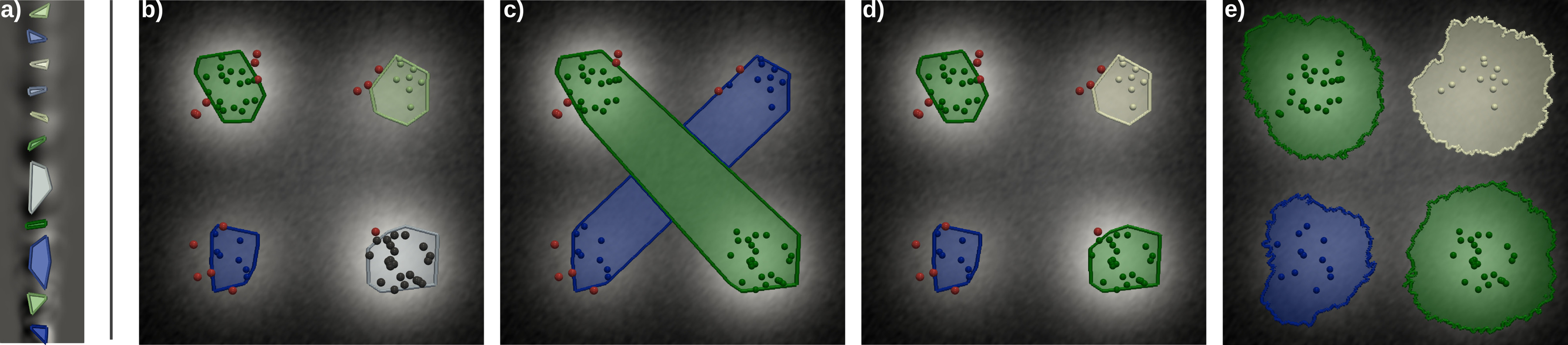
Figure 12: Comparison to alternative critical point clustering strategies. (a) Clustering the critical points directly in the spatial domain can cluster erroneously features which never occur simultaneously in the ensemble but which are close from each other in the spatial domain (dataset from Persistence Atlas for Critical Point Variability in Ensembles). (b) On the contrary, features which always occur simultaneously (Figure 2) may not be clustered together if they are too distant from each other, leading to an overestimated number of clusters (black spheres). (c) Kernel based methods for persistence diagrams [70, 40] do not take spatial embedding into account and cluster together members with the same persistence profile irrespective of the features’ location, leading to an underestimated number of clusters. (d) Even when the clustering is explicitly given, confidence regions based on convex hulls miss 21% of the critical points of the test ensemble (red spheres). (e) The persistence atlas estimated from the training ensemble provides a correct prediction for 100% of the critical points of the test ensemble (colored spheres).

6 Conclusion

In this paper, we presented the Persistence Atlas, an approach for the visual analysis of the spatial variability of features of interest represented by critical points in ensemble data. By analyzing the structure of the ensemble in terms of patterns of critical point layouts, our method addresses trend variability, by identifying clusters of ensemble members which share a common geometrical configuration of critical points. By computing mandatory critical points for each cluster, our approach addresses spatial variability, by showing minimal regions where at least one critical point is guaranteed to occur for each member of the cluster, hence conveying the possible extent of features for each trend. Our approach is based on the new notion of Persistence Map, which describes the local density in critical points and leverages topological persistence to emphasize salient features, and which has been shown to be well suited for the purpose of comparing geometrical layouts of critical points. We showed how to leverage spectral embedding methods to provide low-dimensional views representing the main trends found in the ensemble. We also showed how to leverage spectral clustering to automatically identify revelant clusters of ensemble members and how to provide relevant automatic guesses based on eigengaps for the number of clusters. In practice, our approach has been shown to provide more accurate descriptions of the variability of critical points than global methods, such as the original mandatory critical points [29], which either miss features or considerably over-estimate spatial variability in the presence of trend variability. We quantitatively evaluated the prediction accuracy of our method and showed that it compared favorably to a baseline strategy based on an off-the-shelf clustering approach. Our work extends recent advances in the visual analysis of spatial variability in ensembles of geometrical objects, such as level sets [27] or streamlines [26], to topological structures. In particular, we focused in this paper on features of interest represented by critical points. However, many more topological constructions could benefit from a similar variability analysis based on such tailored clustering strategies. For instance, the separatrices of the Morse-Smale complex [32, 71] have been shown to excel at representing filament structures in various applications, such as chemistry [28, 10] or astrophysics [79, 78], and studying their trend and spatial variabilities would be of tremedous help for the understanding of non-deterministic models in these applications. By first focusing on critical points, we believe we made a first step in this direction, which will be helpful and inspirational for future generalizations to other topological constructions.

- [1] ISO/IEC Guide 98-3:2008 uncertainty of measurement-part 3: Guide to the expression of uncertainty in measurement (GUM), 2008.
- [2] H. Abdi and L. Williams. Principal component analysis. Wiley Interdisciplinary Reviews: Computational Statistics, 2010.
- [3] H. Adams, T. Emerson, M. Kirby, R. Neville, C. Peterson, P. Shipman, S. Chepushtanova, E. Hanson, F. Motta, and L. Ziegelmeier. Persistence images: A stable vector representation of persistent homology. Journal of Machine Learning Research, 2017.
- [4] T. Athawale and A. Entezari. Uncertainty quantification in linear interpolation for isosurface extraction. IEEE Transactions on Visualization and Computer Graphics (Proc. of IEEE VIS), 2013.
- [5] T. Athawale, E. Sakhaee, and A. Entezari. Isosurface visualization of data with nonparametric models for uncertainty. IEEE Transactions on Visualization and Computer Graphics (Proc. of IEEE VIS), 2016.
- [6] T. F. Banchoff. Critical points and curvature for embedded polyhedral surfaces. The American Mathematical Monthly, 1970.
- [7] U. Bauer, X. Ge, and Y. Wang. Measuring distance between Reeb graphs. In Symp. on Comp. Geom., 2014.
- [8] K. Beketayev, D. Yeliussizov, D. Morozov, G. H. Weber, and B. Hamann. Measuring the distance between merge trees. In Topological Methods in Data Analysis and Visualization III, Theory, Algorithms, and Applications. 2014.
- [9] M. Belkin and P. Niyogi. Laplacian eigenmaps for dimensionality reduction and data representation. Neural Computation, 2003.
- [10] H. Bhatia, A. G. Gyulassy, V. Lordi, J. E. Pask, V. Pascucci, and P.-T. Bremer. Topoms: Comprehensive topological exploration for molecular and condensed-matter systems. Journal of Computational Chemistry, 2018.
- [11] H. Bhatia, S. Jadhav, P. Bremer, G. Chen, J. Levine, L. Nonato, and V. Pascucci. Flow visualization with quantified spatial and temporal errors using edge maps. IEEE Transactions on Visualization and Computer Graphics, 18(9):1383–1396, 2012.
- [12] G.-P. Bonneau, H.-C. Hege, C. Johnson, M. M. Oliveira, K. Potter, and P. Rheingans. Overview and State-of-the-Art of Uncertainty Visualization. In Scientific Visualization: Uncertainty, Multifield, Biomedical, Scalable, Mathematics and Visualization. Springer, 2014.
- [13] I. Borg and P. Groenen. Modern multidimensional scaling: Theory and Applications. Springer, 2005.
- [14] M. B. Botnan and H. B. Bjerkevik. Computational complexity of the interleaving distance. In Symp. on Comp. Geom., 2018.
- [15] P. Bremer, G. Weber, J. Tierny, V. Pascucci, M. Day, and J. Bell. Interactive exploration and analysis of large scale simulations using topology-based data segmentation. IEEE Transactions on Visualization and Computer Graphics, 2011.
- [16] S. Bruckner and T. Möller. Isosurface similarity maps. Computer Graphics Forum (Proc. of EuroVis), 2010.
- [17] M. Carrière, M. Cuturi, and S. Oudot. Sliced wasserstein kernel for persistence diagrams. In ICML, 2017.
- [18] F. Chazal, D. Cohen-Steiner, M. Glisse, L. J. Guibas, and S. Oudot. Proximity of persistence modules and their diagrams. In Symp. on Comp. Geom., 2009.
- [19] F. Chazal, L. Guibas, S. Oudot, and P. Skraba. Persistence-based clustering in Riemannian manifolds. Journal of the ACM, 2013.
- [20] D. Cohen-Steiner, H. Edelsbrunner, and J. Harer. Stability of persistence diagrams. In Symp. on Comp. Geom., 2005.
- [21] P. Diggle, P. Heagerty, K.-Y. Liang, and S. Zeger. Analysis of longitudinal data. Oxford University Press, 2002.
- [22] H. Edelsbrunner and J. Harer. Computational Topology: An Introduction. American Mathematical Society, 2009.
- [23] H. Edelsbrunner, D. Letscher, and A. Zomorodian. Topological persistence and simplification. Disc. Compu. Geom., 2002.
- [24] H. Edelsbrunner and E. P. Mucke. Simulation of simplicity: a technique to cope with degenerate cases in geometric algorithms. ACM Trans. on Graph., 1990.
- [25] G. Favelier, C. Gueunet, and J. Tierny. Visualizing ensembles of viscous fingers. In IEEE SciVis Contest, 2016.
- [26] F. Ferstl, K. Bürger, and R. Westermann. Streamline variability plots for characterizing the uncertainty in vector field ensembles. IEEE Transactions on Visualization and Computer Graphics (Proc. of IEEE VIS), 2016.
- [27] F. Ferstl, M. Kanzler, M. Rautenhaus, and R. Westermann. Visual analysis of spatial variability and global correlations in ensembles of iso-contours. Computer Graphics Forum (Proc. of EuroVis), 2016.
- [28] D. Guenther, R. Alvarez-Boto, J. Contreras-Garcia, J.-P. Piquemal, and J. Tierny. Characterizing molecular interactions in chemical systems. IEEE Transactions on Visualization and Computer Graphics (Proc. of IEEE VIS), 2014.
- [29] D. Guenther, J. Salmon, and J. Tierny. Mandatory critical points of 2D uncertain scalar fields. Computer Graphics Forum (Proc. of EuroVis), 2014.
- [30] C. Gueunet, P. Fortin, J. Jomier, and J. Tierny. Task-based Augmented Merge Trees with Fibonacci Heaps,. In IEEE LDAV, 2017.
- [31] A. Gyulassy, P. Bremer, R. Grout, H. Kolla, J. Chen, and V. Pascucci. Stability of dissipation elements: A case study in combustion. Computer Graphics Forum (Proc. of EuroVis), 2014.
- [32] A. Gyulassy, P. T. Bremer, B. Hamann, and V. Pascucci. A practical approach to morse-smale complex computation: Scalability and generality. IEEE Transactions on Visualization and Computer Graphics (Proc. of IEEE VIS), 2008.
- [33] A. Gyulassy, M. A. Duchaineau, V. Natarajan, V. Pascucci, E. Bringa, A. Higginbotham, and B. Hamann. Topologically clean distance fields. IEEE Transactions on Visualization and Computer Graphics (Proc. of IEEE VIS), 2007.
- [34] A. Gyulassy, A. Knoll, K. Lau, B. Wang, P. Bremer, M. Papka, L. A. Curtiss, and V. Pascucci. Interstitial and interlayer ion diffusion geometry extraction in graphitic nanosphere battery materials. IEEE Transactions on Visualization and Computer Graphics (Proc. of IEEE VIS), 2015.
- [35] C. Heine, H. Leitte, M. Hlawitschka, F. Iuricich, L. De Floriani, G. Scheuermann, H. Hagen, and C. Garth. A survey of topology-based methods in visualization. Comp. Grap. For., 2016.
- [36] M. Hilaga, Y. Shinagawa, T. Kohmura, and T. L. Kunii. Topology matching for fully automatic similarity estimation of 3D shapes. In Proc. of ACM SIGGRAPH, 2001.
- [37] M. Hummel, H. Obermaier, C. Garth, and K. I. Joy. Comparative visual analysis of lagrangian transport in CFD ensembles. IEEE Transactions on Visualization and Computer Graphics (Proc. of IEEE VIS), 2013.
- [38] C. Johnson and A. Sanderson. A next step: Visualizing errors and uncertainty. IEEE Computer Graphics and Applications, 2003.
- [39] J. Kasten, J. Reininghaus, I. Hotz, and H. Hege. Two-dimensional time-dependent vortex regions based on the acceleration magnitude. IEEE Transactions on Visualization and Computer Graphics, 2011.
- [40] R. Kwitt. Persistence learning. https://github.com/rkwitt/persistence-learning, 2015.
- [41] D. E. Laney, P. Bremer, A. Mascarenhas, P. Miller, and V. Pascucci. Understanding the structure of the turbulent mixing layer in hydrodynamic instabilities. IEEE Transactions on Visualization and Computer Graphics (Proc. of IEEE VIS), 2006.
- [42] T. Liebmann and G. Scheuermann. Critical points of gaussian-distributed scalar fields on simplicial grids. Computer Graphics Forum (Proc. of EuroVis), 2016.
- [43] S. P. Lloyd. Least square quantization in pcm. Technical report, Bell Telephone Laboratories, 1957.
- [44] A. M. MacEachren, A. Robinson, S. Hopper, S. Gardner, R. Murray, M. Gahegan, and E. Hetzler. Visualizing geospatial information uncertainty: What we know and what we need to know. Cartography and Geographic Information Science, 32(3):139–160, 2005.
- [45] J. B. MacQueen. Some methods for classification and analysis of multivariate observations. In Proc. Symposium on Mathematical Statistics and Probability, 1967.
- [46] J. Milnor. Morse Theory. Princeton U. Press, 1963.
- [47] M. Mirzargar, R. T. Whitaker, and R. M. Kirby. Curve boxplot: Generalization of boxplot for ensembles of curves. IEEE Transactions on Visualization and Computer Graphics (Proc. of IEEE VIS), 2014.
- [48] J. Munkres. Algorithms for the assignment and transportation problems. Journal of the Society for Industrial and Applied Mathematics, 1957.
- [49] G. Nucha, G. Bonneau, S. Hahmann, and V. Natarajan. Computing contour trees for 2d piecewise polynomial functions. Computer Graphics Forum (Proc. of EuroVis), 2017.
- [50] S. Oeltze, D. J. Lehmann, A. Kuhn, G. Janiga, H. Theisel, and B. Preim. Blood flow clustering and applications invirtual stenting of intracranial aneurysms. IEEE Transactions on Visualization and Computer Graphics (Proc. of IEEE VIS), 2014.
- [51] M. Otto, T. Germer, H.-C. Hege, and H. Theisel. Uncertain 2D vector field topology. Comp. Graph. For., 29:347–356, 2010.
- [52] M. Otto, T. Germer, and H. Theisel. Uncertain topology of 3d vector fields. In Proc. of IEEE PacificVis, 2011.
- [53] A. T. Pang, C. M. Wittenbrink, and S. K. Lodha. Approaches to uncertainty visualization. The Visual Computer, 13(8):370–390, 1997.
- [54] F. Pedregosa, G. Varoquaux, A. Gramfort, V. Michel, B. Thirion, O. Grisel, M. Blondel, P. Prettenhofer, R. Weiss, V. Dubourg, J. VanderPlas, A. Passos, D. Cournapeau, M. Brucher, M. Perrot, and E. Duchesnay. Scikit-learn: Machine learning in python. Journal of Machine Learning Research, 2011.
- [55] D. Pelleg and A. W. Moore. X-means: Exteding k-means with efficient estimation of the number of clusters. In Proc. of ICML, 2000.
- [56] C. Petz, K. Pöthkow, and H.-C. Hege. Probabilistic local features in uncertain vector fields with spatial correlation. Computer Graphics Forum (Proc. of EuroVis), 31(3pt2):1045–1054, 2012.
- [57] T. Pfaffelmoser, M. Mihai, and R. Westermann. Visualizing the variability of gradients in uncertain 2d scalar fields. IEEE Transactions on Visualization and Computer Graphics, 2013.
- [58] T. Pfaffelmoser, M. Reitinger, and R. Westermann. Visualizing the positional and geometrical variability of isosurfaces in uncertain scalar fields. Computer Graphics Forum (Proc. of EuroVis), 30:951–960, 2011.
- [59] T. Pfaffelmoser and R. Westermann. Visualization of global correlation structures in uncertain 2d scalar fields. Computer Graphics Forum (Proc. of EuroVis), 2012.
- [60] T. Pfaffelmoser and R. Westermann. Visualizing contour distributions in 2d ensemble data. In EuroVis-Short Papers, pp. 55–59. The Eurographics Association, 2013.
- [61] J. M. Phillips, B. Wang, and Y. Zheng. Geometric inference on kernel density estimates. In Symp. on Comp. Geom., 2015.
- [62] K. Pöthkow and H.-C. Hege. Positional uncertainty of isocontours: Condition analysis and probabilistic measures. IEEE Transactions on Visualization and Computer Graphics, 17(10):1393–1406, 2011.
- [63] K. Pöthkow and H.-C. Hege. Nonparametric models for uncertainty visualization. Computer Graphics Forum (Proc. of EuroVis), 32:131–140, 2013.
- [64] K. Pöthkow, C. Petz, and H.-C. Hege. Approximate level-crossing probabilities for interactive visualization of uncertain isocontours. Int. J. Uncert. Quantif., 3:101–117, 2013.
- [65] K. Pöthkow, B. Weber, and H. Hege. Probabilistic marching cubes. Computer Graphics Forum (Proc. of EuroVis), 2011.
- [66] K. Potter, S. Gerber, and E. Anderson. Visualization of uncertainty without a mean. IEEE CGA, 33:75–79, 2013.
- [67] K. Potter, P. Rosen, and C. R. Johnson. From quantification to visualization: A taxonomy of uncertainty visualization approaches. In Uncertainty Quantification in Scientific Computing, vol. 377, pp. 226–249. Springer, 2012.
- [68] K. Potter, A. T. Wilson, P. Bremer, D. N. Williams, C. M. Doutriaux, V. Pascucci, and C. R. Johnson. Ensemble-vis: A framework for the statistical visualization of ensemble data. In IEEE International Conference on Data Mining Workshops, 2009.
- [69] P. S. Quinan and M. D. Meyer. Visually comparing weather features in forecasts. IEEE Transactions on Visualization and Computer Graphics, 2016.
- [70] J. Reininghaus, S. Huber, U. Bauer, and R. Kwitt. A stable multi-scale kernel for topological machine learning. In IEEE CVPR, 2015.
- [71] V. Robins, P. Wood, and A. Sheppard. Theory and algorithms for constructing discrete morse complexes from grayscale digital images. IEEE Trans. on Pat. Ana. and Mach. Int., 2011.
- [72] H. Saikia, H. Seidel, and T. Weinkauf. Extended branch decomposition graphs: Structural comparison of scalar data. Computer Graphics Forum (Proc. of EuroVis), 2014.
- [73] J. Sanyal, S. Zhang, J. Dyer, A. Mercer, P. Amburn, and R. J. Moorhead. Noodles: A tool for visualization of numerical weather model ensemble uncertainty. IEEE Transactions on Visualization and Computer Graphics (Proc. of IEEE VIS), 2010.
- [74] G. Scheuermann, X. Tricoche, and H. Hagen. C1-interpolation for vector field topology visualization. In IEEE VIS, 1999.
- [75] S. Schlegel, N. Korn, and G. Scheuermann. On the interpolation of data with normally distributed uncertainty for visualization. IEEE Transactions on Visualization and Computer Graphics (Proc. of IEEE VIS), 2012.
- [76] I. SciVisContest. Simulation of the isabel hurricane. http://sciviscontest-staging.ieeevis.org/2004/data.html.
- [77] J. Shi and J. Malik. Normalized cuts and image segmentation. In Proc. of IEEE CVPR, 1997.
- [78] N. Shivashankar, P. Pranav, V. Natarajan, R. van de Weygaert, E. P. Bos, and S. Rieder. Felix: A topology based framework for visual exploration of cosmic filaments. IEEE Transactions on Visualization and Computer Graphics, 2016. http://vgl.serc.iisc.ernet.in/felix/index.html.
- [79] T. Sousbie. The persistent cosmic web and its filamentary structure: Theory and implementations. Royal Astronomical Society, 2011. http://www2.iap.fr/users/sousbie/web/html/indexd41d.html.
- [80] A. Szymczak. Hierarchy of stable morse decompositions. IEEE Transactions on Visualization and Computer Graphics, 19(5):799–810, 2013.
- [81] J. B. Tenenbaum, V. de Silva, and J. Langford. A global geometric framework for nonlinear dimensionality reduction. Science, 2000.
- [82] D. M. Thomas and V. Natarajan. Multiscale symmetry detection in scalar fields by clustering contours. IEEE Transactions on Visualization and Computer Graphics (Proc. of IEEE VIS), 2014.
- [83] J. Tierny, G. Favelier, J. A. Levine, C. Gueunet, and M. Michaux. The Topology ToolKit. IEEE Transactions on Visualization and Computer Graphics (Proc. of IEEE VIS), 2017. https://topology-tool-kit.github.io/.
- [84] K. Turner, Y. Mileyko, S. Mukherjee, and J. Harer. Fréchet means for distributions of persistence diagrams. Discrete & Computational Geometry, 2014.
- [85] U. von Luxburg. A tutorial on spectral clustering. In Statistics and Computing, 2007.
- [86] R. T. Whitaker, M. Mirzargar, and R. M. Kirby. Contour boxplots: A method for characterizing uncertainty in feature sets from simulation ensembles. IEEE Transactions on Visualization and Computer Graphics (Proc. of IEEE VIS), 2013.
- [87] F. Wickelmaier. An introduction to mds. Technical report, Aalborg University, 2003.