Connected and disconnected contributions to nucleon axial form factors using $N_{f}=2$ twisted mass fermions at the physical point

Abstract

We present results on the isovector and isoscalar nucleon axial form factors including disconnected contributions, using an ensemble of $N_{f}=2$ twisted mass clover-improved Wilson fermions simulated with approximately the physical value of the pion mass. The light disconnected quark loops are computed using exact deflation, while the strange and the charm quark loops are evaluated using the truncated solver method. Techniques such as the summation and the two-state fits have been employed to access ground-state dominance.

1 Introduction

The form factors of the nucleon are important quantities that encapsulate information about its structure and properties. Contrary to the electromagnetic form factors that are well determined experimentally, the axial form factors are less known. The axial charge of the nucleon is an exception since it can be measured to high precision from $\beta$-decays. The momentum dependence of the axial form factors can be extracted from elastic scattering of neutrinos and protons Ahrens:1988rr . The induced pseudoscalar form factor has been measured experimentally only for few values of momentum transfer Choi:1993vt from the cross section for exclusive $\pi^{+}$ electroproduction on the proton.

In this work, we evaluate the nucleon axial $G_{A}(Q^{2})$ and induced pseudoscalar $G_{p}(Q^{2})$ form factors using an ensemble of $N_{f}=2$ twisted mass clover-improved Wilson ensemble with light quark mass tuned to approximately reproduce the physical value of the pion mass Abdel-Rehim:2015pwa . Both connected and disconnected contributions are evaluated allowing to compute the isovector, isoscalar as well as strange and charm form factors.

2 Lattice Formulation

2.1 Axial form factors

The decomposition of the nucleon matrix element of the axial-vector current $A_{\mu}(x)$ in Euclidean time is given by

$$\langle N(p^{\prime},s^{\prime})|A_{\mu}|N(p,s)\rangle=i\sqrt{\frac{m_{N}^{2}}{E_{N}(\vec{p}^{\prime})E_{N}(\vec{p})}}\bar{u}_{N}(p^{\prime},s^{\prime})\left(\gamma_{\mu}G_{A}(Q^{2})-i\frac{Q_{\mu}}{2m_{N}}G_{p}(Q^{2})\right)\gamma_{5}u_{N}(p,s),$$ (1)

where $p,s$ ($p^{\prime},s^{\prime}$) are the momentum and spin of the initial (final) nucleon state, $N$ is the nucleon state, $u_{N}$ the nucleon spinor, $m_{N}$ and $E_{N}(\vec{p})$ are the nucleon mass and energy with momentum $\vec{p}$ and $Q^{2}=(p^{\prime}-p)^{2}$ the momentum transfer square. We consider the isovector, isoscalar as well as strange and charm combinations

$$A^{\rm u-d}_{\mu}=\bar{\psi}(x)\gamma_{\mu}\gamma_{5}\frac{\tau^{3}}{2}\psi(x),\,\,A^{\rm u+d}_{\mu}=\bar{\psi}(x)\gamma_{\mu}\gamma_{5}\mathbbm{1}\psi(x),\,\,A^{s}_{\mu}=\bar{s}(x)\gamma_{\mu}\gamma_{5}s(x)\,\,\,\textrm{and}\,\,\,A^{c}_{\mu}=\bar{c}(x)\gamma_{\mu}\gamma_{5}c(x),$$ (2)

where $\tau^{3}$ is the Pauli matrix acting in flavor space.

2.2 Lattice extraction

Computation of two- and three-point correlation functions is needed to extract nucleon matrix elements. The three-point functions receive contributions from the so-called connected and disconnected diagrams. For the isovector combination disconnected contributions cancel out in the isospin limit. For the connected contributions we employ the standard fixed-sink method where sequential inversions through the sink are performed. Deflation of the low modes is employed to accelerate the inversion of the Dirac operator. For the disconnected quark loops we combined the one-end trick McNeile:2006bz with the truncated solver method (TSM) Bali:2009hu to reduce the computational cost. Two-point functions are computed for several source positions per configuration to increase the statistical accuracy.

We construct the following ratio of the appropriate three-point function $G_{\mu}(\Gamma_{\nu},\vec{p}\,^{\prime},\vec{p};t_{s},t_{\rm ins})$ to two-functions $C(\Gamma_{0},\vec{p},t)$

$$R_{\mu}(\Gamma_{\nu},\vec{p}\,^{\prime},\vec{p};t_{s},t_{\rm ins})=\frac{G_{\mu}(\Gamma_{\nu},\vec{p}\,^{\prime},\vec{p};t_{s},t_{\rm ins})}{C(\Gamma_{0},\vec{p}\,^{\prime};t_{s})}\sqrt{\frac{C(\Gamma_{0},\vec{p};t_{s}-t_{\rm ins})C(\Gamma_{0},\vec{p}\,^{\prime};t_{\rm ins})C(\Gamma_{0},\vec{p}\,^{\prime};t_{s})}{C(\Gamma_{0},\vec{p}\,^{\prime};t_{s}-t_{\rm ins})C(\Gamma_{0},\vec{p};t_{\rm ins})C(\Gamma_{0},\vec{p};t_{s})}},$$ (3)

which, in the large time limit $t_{s}-t_{\rm ins}\gg 1$ and $t_{\rm ins}\gg 1$ yields the desired nucleon matrix element. The insertion time $t_{\rm ins}$ as well as the sink time $t_{s}$ are taken relative to the source. To determine, if indeed, these time separations are large enough we employ three methods: i) plateau method, which assumes that the ratio of Eq. (3) is dominated by the ground state and perform a constant fit as a function of $t_{\rm ins}$ to extract the matrix element, ii) summation method, in which one sums over $t_{\rm ins}$ and extracts the matrix element from the slope of a linear fit, and iii) two-state fit method which includes besides the ground state the first excited state in the fit to extract the matrix element. We require that these three methods give consistent results for the matrix element.

We perform a non-perturbative calculation of both the renormalization functions for the isovector and isoscalar currents needed for the extraction of physical matrix elements from lattice results using the Rome-Southampton method Martinelli:1994ty . Lattice artifacts are subtracted perturbatively to ${\cal O}(a^{2})$ Alexandrou:2015sea to yield a better determination of the limit $(ap)^{2}\rightarrow 0$. We take the chiral limit to extract the renormalization functions. We find for the non-singlet case $Z_{A}^{ns}=0.7910(4)(5)$ and for the singlet $Z_{A}^{s}=0.7968(25)(91)$, which are compatible within errors.

2.3 Lattice Setup and Statistics

We analyze an ensemble of $N_{f}=2$ twisted mass clover improved Wilson fermions with pion mass $m_{\pi}=0.1304(4)$ GeV on a lattice of size $48^{3}\times 96$ and a lattice spacing $a$=0.0938(3) fm determined from nucleon mass Alexandrou:2017xwd . In Tab. 1 we give the statistics used for the computation of connected and disconnected contributions. For the connected, three values of $t_{s}$ analyzed in the frame where $\vec{p}^{\prime}=\vec{0}$, while for the disconnected all separations are available without additional cost in both the rest frame of the final nucleon as well as for $\vec{p}^{\prime}=\frac{2\pi\hat{\vec{n}}}{L}$. We note the much larger number of configurations and source positions analyzed for the evaluation of the disconnected contributions.

Connected			Disconnected
$t_{s}/a$	$N_{\rm conf}$	$N_{\rm src}$	Flavor	$N_{\rm conf}$	$N_{r}^{\rm HP}$	$N_{r}^{\rm LP}$	$N_{\rm src}$
10	579	16	light	2120	2250	-	100
12	579	16	strange	2057	63	1024	100
14	579	16	charm	2034	5	1250	100

Table 1: Statistics used in this study. $N_{\rm conf}$ is the number of gauge configurations and $N_{\rm src}$ is the number of source positions per configuration. For the disconnected contributions, $N_{r}^{\rm HP}$ is the number of high-precision stochastic vectors produced, and $N_{r}^{\rm LP}$ is the number of low-precision vectors used when the TSM has been used.

3 Results

3.1 Axial charge

At zero momentum transfer the matrix element of the axial-vector current yields the nucleon axial charge $g_{A}\equiv g_{A}^{u-d}$ (isovector) and $g_{A}^{u+d}$ (isoscalar). In Fig. 1 we present our results for both quantities showing separately the connected and disconnected contributions in the case of $g_{A}^{u+d}$. The ratio for the connected contributions is computed at three values of $t_{s}$. We check that the values extracted using the plateau, summation and two-state methods are consistent as shown in Fig. 1. We include a systematic error due to the excited states taken as the difference between the plateau value that demonstrates convergence with $t_{s}$ and the one extracted from the two-state fit. We quote these values in Tab. 2.

$g_{A}$	$g_{A}^{u+d}$ (Conn.)	$g_{A}^{u+d}$ (Disc.)	$g_{A}^{u+d}$	$g_{A}^{s}$	$g_{A}^{c}$
1.212(33)(22)	0.595(28)(1)	-0.150(20)(19)	0.445(34)(19)	-0.0427(100)(93)	-0.00338(188)(667)

Table 2: Our values for the nucleon axial charges. The first error is statistical and the second is a systematic due to the excited states contamination.

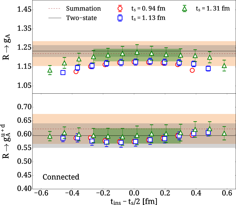
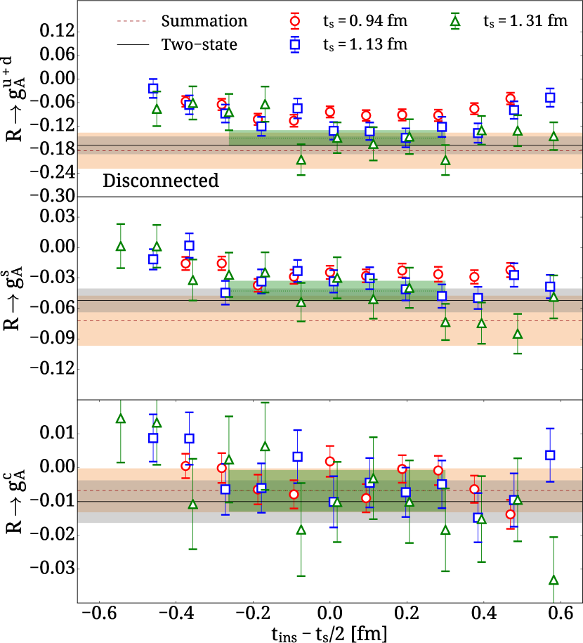
Figure 1: Left: Ratio from where we extract $g_{A}$ and the connected contributions to $g_{A}^{u+d}$. Results are presented for three values of $t_{s}$, namely $t_{s}=0.94,\;1.13$ and 1.31 fm shown with open red circles, open blue squares and open green triangles, respectively. The constant fit using the plateau method is shown with the dotted line spanning the selected fit range of $t_{\rm ins}$ and its corresponding error band. Results extracted from the summation method are shown with the brown dashed line and corresponding error band, while results using two-state fits are shown with the solid black line spanning the entire horizontal axis. Right: Ratio from where we extract the disconnected contributions to $g_{A}^{u+d}$, $g_{A}^{s}$ and $g_{A}^{c}$. The convention is as the left panel.

3.2 Isovector Axial and induced pseudoscalar form factors

In Fig. 2 we show results for the isovector $G_{A}$ and $G_{p}$. For the axial form factor we fit our results to a dipole form: $G_{A}(Q^{2})=\frac{g_{A}}{(1+Q^{2}/m_{A}^{2})^{2}}$ where $g_{A}$ is fixed by the value of the form factor at zero momentum transfer and the axial mass $m_{A}$ is allowed to vary. We find an axial mass $m_{A}=1.322(42)(17)$ GeV, which is consistent with the recent experimental value AguilarArevalo:2010zc from MiniBooNE experiment but larger than the one extracted from previous experiments. For the induced pseudoscalar form factor we fit to a pole form $G_{p}(Q^{2})=G_{A}(Q^{2})\frac{C}{Q^{2}+m_{p}^{2}}$ where $C$ and $m_{p}$ are fit parameters. As shown in Fig. 2 our lattice results display a milder $Q^{2}$-dependence compared to the one expected from the pion pole dominance. This discrepancy at low $Q^{2}$ values might be due to volume effects that suppress pion cloud formation and need to be investigated in future studies using bigger volumes and better interpolating fields.

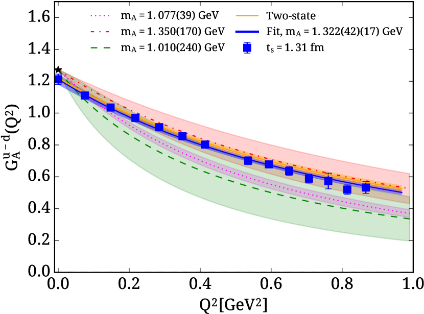
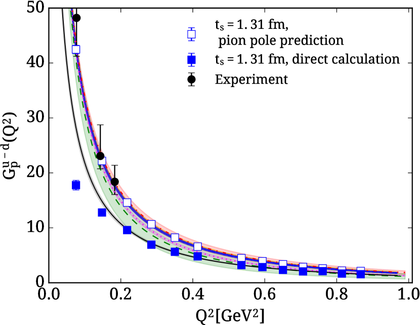
Figure 2: Results for $G_{A}^{u-d}(Q^{2})$ and $G_{p}^{u-d}(Q^{2})$ using values extracted from the plateau method at $t_{s}=1.31$ fm (filled blue squares). In the left panel, the solid blue (orange) line shows the fit to our results extracted from the plateau (two-state fit) using dipole form. Black asterisk shows the experimental value of $g_{A}$. The purple, red and green bands are experimental results for $G_{A}^{u-d}(Q^{2})$ taken from Refs. Liesenfeld:1999mv , AguilarArevalo:2010zc and Meyer:2016oeg respectively. For the induced pseudoscalar, the open blue squares show the pion-pole prediction results to $G_{p}^{u-d}(Q^{2})$ from our lattice results of $G_{A}^{u-d}(Q^{2})$ together with the corresponding fits, blue (orange) band is a fit extracted from the plateau (two-state) fit. The filled blue squares show $G_{p}^{u-d}(Q^{2})$ extracted directly from the nucleon matrix element with a pole fit (solid black line) after omitting the two lowest $Q^{2}$ values. The filled black circles are experimental results of $G_{p}^{u-d}(Q^{2})$ from Ref. Choi:1993vt . The purple, red and green bands are constructed using the experimental results for $G_{A}^{u-d}(Q^{2})$ and pion pole to infer $G_{p}^{u-d}(Q^{2})$.

3.3 Disconnected contributions to the axial form factors

In Fig. 3 we show the disconnected contributions to the isoscalar $G_{A}^{u+d}$ and $G_{p}^{u+d}$ as well as the strange $G_{A}^{s}$ and $G_{p}^{s}$ form factors. We perform a model independent fit to these data using the z-expansion Hill:2010yb that yields a good description of the $Q^{2}$-dependence.

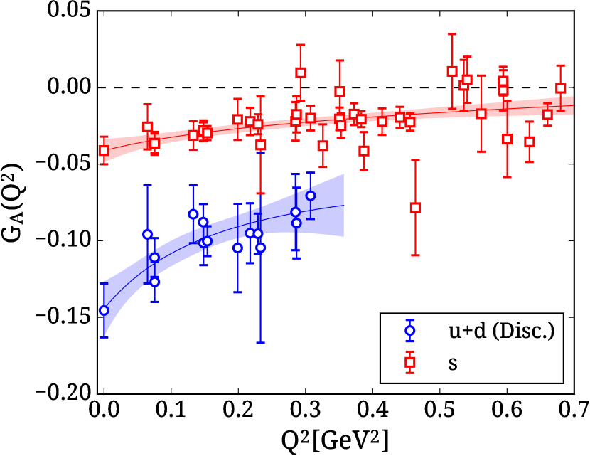
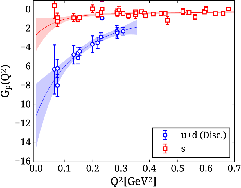
Figure 3: Results for the disconnected contributions: Left $G_{A}^{u+d}(Q^{2})$ (red) and $G_{A}^{s}(Q^{2})$ (blue. Right: $G_{p}(Q^{2})^{u+d}$ (red) and $G_{p}^{s}(Q^{2})$ (blue). The lattice results are extracted from the plateau method at $t_{s}=1.31$ fm. The bands show the fit using the z-expansion.

In Fig. 4 we show our results for $G_{A}^{c}(Q^{2})$ extracted from the plateau method for a source-sink time separation $t_{s}=0.94$ fm. Due to the fact that the statistical uncertainty for this quantity is large it is not possible to study larger separations. $G_{A}^{c}(Q^{2})$ is clearly negative and non-zero, with values that are an order of magnitude smaller as compared to $G_{A}^{s}(Q^{2})$. The z-expansion requires high accuracy and thus we fit the $Q^{2}$-dependence using a dipole form. $G_{p}^{c}(Q^{2})$ is very noisy to display and it is omitted.

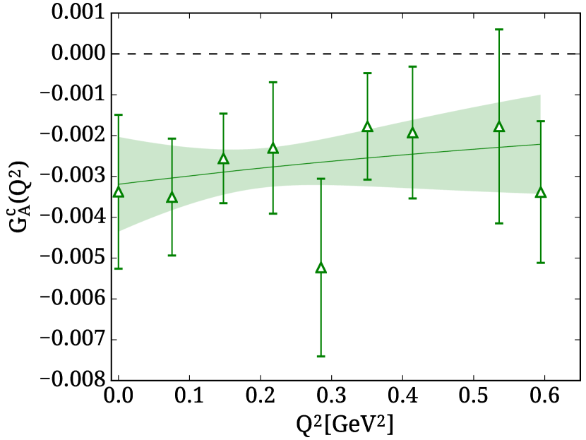
Figure 4: Results for $G_{A}^{c}(Q^{2})$ extracted using the plateau method at $t_{s}=0.94$ fm. The fit is performed using a dipole form.

3.4 Isoscalar Axial and induced pseudoscalar form factors

Having both connected and disconnected contributions allows us to compute the total contribution to the isoscalar form factor. In Fig. 5 we show results for the isoscalar $G_{A}^{u+d}$. As can be seen, the disconnected contribution comes with a different sign compared to the connected one, it is clearly non-zero and changes the $Q^{2}$-dependence of the form factor. Only after we include the disconnected contribution we have agreement with the experimental value of $g_{A}^{u+d}$. The isoscalar mass $m_{A}^{u+d}=1.736(244)(374)$ is higher than the one extracted from the isovector case as expected from the smoother $Q^{2}$-dependence observed of the isoscalar form factor.

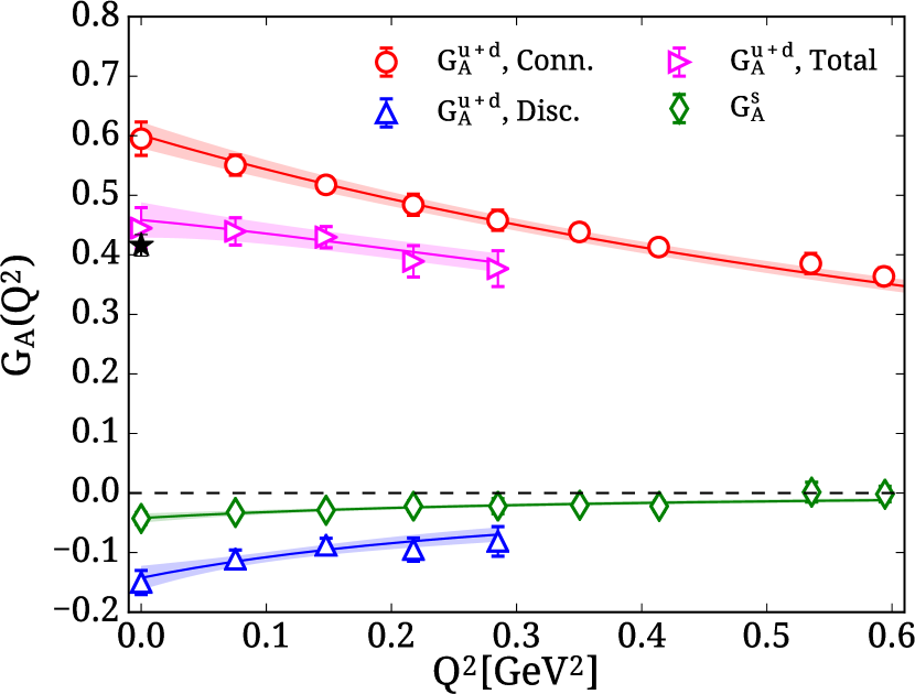
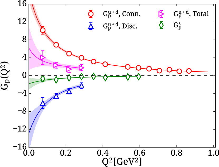
Figure 5: Results for the isoscalar $G_{A}^{u+d}(Q^{2})$ and $G_{A}^{s}(Q^{2})$ (left) and $G_{p}^{u+d}(Q^{2})$ and $G_{p}^{s}(Q^{2})$ (right). Connected contributions to the isoscalar form factors are shown by the red open circles, disconnected by the blue upper open triangles, and the total by the right magenta open triangles. The strange form factors are shown by the green rhombus. The black star shows the experimental value of $g_{A}^{u+d}$.

Our results on the isoscalar $G_{p}^{u+d}$ are presented in Fig. 5. What is remarkable is the large disconnected contribution to the induced pseudoscalar form factor, which is of the same order as the connected but with the opposite sign. Fitting separately the two contributions we find consistent pole masses, namely $m_{p}^{\rm u+d,\;conn}=0.324(22)(12)$ GeV and $m_{p}^{\rm u+d,\;disc}=0.331(81)(36)$ showing that the two contributions are dominated by the same pole mass canceling the pion mass dependence in the isoscalar form factor.

3.5 Comparison with other recent lattice QCD results

In Fig. 6 we show a comparison of our results at the physical point with results from another study at a higher pion mass that used $N_{f}=2+1$ clover-improved Wilson fermions Green:2017keo with pion mass of 317 MeV. As can be seen, the values of $G_{A}^{u-d}(Q^{2})$ are consistently larger as compared to ours in particular at larger values of $Q^{2}$ leading to a milder slope than ours. Assuming that lattice artifacts are small in both calculations this indicates a non-zero pion mass dependence. There is an overall agreement between results on $G_{A}^{s}(Q^{2})$ Fig. 6 with the exception of the value at $Q^{2}=0$. We note that the results from Ref. Green:2017keo used a smaller source-sink time separation. This together with the fact that the pion mass is larger than physical is reflected in having smaller statistical errors even though our statistics are twice as large.

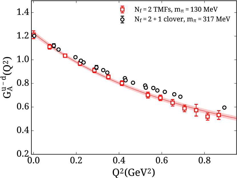
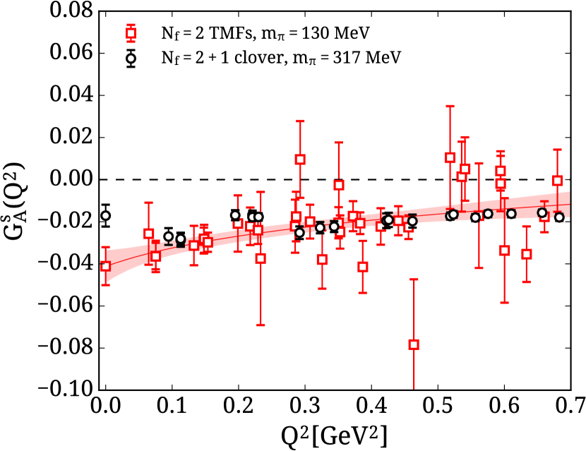
Figure 6: Comparison of our results on $G_{A}^{u-d}(Q^{2})$ (left) and $G_{A}^{s}(Q^{2})$ (right) using twisted mass fermions (TMFs) with approximately a physical value of the light quark mass Alexandrou:2017hac (open red squares) with results using $N_{f}=2+1$ clover fermions  Green:2017keo with light quark mass yielding pion mass of 317 MeV (open black circles). The red band shows the fit to our results with its jackknife error.

4 Conclusions

The isovector, isoscalar, strange and charm axial and induced pseudoscalar form factors of the nucleon are presented using an ensemble of two degenerate dynamical quarks with mass tuned to approximately reproduce the physical value of the pion mass (physical point) Alexandrou:2017hac . Disconnected contributions are evaluated for the first time at the physical point using improved methods providing accurate results. They are shown to be non-zero and of opposite sign to the connected contribution. For the case of the induced pseudoscalar form factor the disconnected are of the same magnitude as the connected canceling the pion pole in the isoscalar $G_{p}^{u+d}(Q^{2})$. Only after adding the disconnected contribution to the isoscalar axial charge we have agreement with the experimental value. Additionally, $G_{A}^{s}(Q^{2})$ and $G_{A}^{c}(Q^{2})$ are found to be non-zero and negative, as is $G_{p}^{s}(Q^{2})$, while $G_{p}^{c}(Q^{2})$ is very noisy.

The value of the nucleon axial charge is lower by one standard deviation as compared to the experimental value and the slope of $G_{A}^{u-d}(Q^{2})$ is milder but in agreement with the experimental result from Ref. AguilarArevalo:2010zc . However, one needs to study the $Q^{2}$-dependence further since lattice QCD results tend to underestimate the slope. $G_{p}^{u-d}(Q^{2})$ also displays a milder $Q^{2}$-dependence than expected from pion pole dominance. We are currently investigating volume effects on these quantities using an ensemble with the same parameters as the one analyzed here but with a lattice size of $64^{3}\times 128$.

Acknowledgments: We acknowledge funding from the European Unionâs Horizon 2020 research and innovation programme under the Marie Sklodowska-Curie grant agreement No 642069. This work was partly supported by a grant from the Swiss National Supercomputing Centre (CSCS) under project IDs s540 and s625 on the Piz Daint system, by a Gauss allocation on SuperMUC with ID 44060 and in addition used computational resources from the John von Neumann-Institute for Computing on the Jureca and the BlueGene/Q Juqueen systems at the research center in Julich. We also acknowledge PRACE for awarding us access to the Tier-0 computing resources Curie, Fermi and SuperMUC based in CEA, France, Cineca, Italy and LRZ, Germany, respectively. K. H. and Ch. K. acknowledge support from the Cyprus Research Promotion Foundation under contract T$\Pi$E/$\Pi\Lambda$HPO/0311(BIE)/09. We also acknowledge financial support from the PRACE-4IP project with grant number 653838.

References

- (1) L.A. Ahrens et al., Phys. Lett. B202, 284 (1988)
- (2) S. Choi et al., Phys. Rev. Lett. 71, 3927 (1993)
- (3) A. Abdel-Rehim et al. (ETM), Phys. Rev. D95, 094515 (2017), 1507.05068
- (4) C. McNeile, C. Michael (UKQCD), Phys. Rev. D73, 074506 (2006), hep-lat/0603007
- (5) G. Bali, S. Collins, A. Schafer, Comput. Phys. Commun. 181, 1570 (2010), 0910.3970
- (6) G. Martinelli, C. Pittori, C.T. Sachrajda, M. Testa, A. Vladikas, Nucl. Phys. B445, 81 (1995), hep-lat/9411010
- (7) C. Alexandrou, M. Constantinou, H. Panagopoulos (ETM), Phys. Rev. D95, 034505 (2017), 1509.00213
- (8) C. Alexandrou, C. Kallidonis, Phys. Rev. D96, 034511 (2017), 1704.02647
- (9) A.A. Aguilar-Arevalo et al. (MiniBooNE), Phys. Rev. D81, 092005 (2010), 1002.2680
- (10) A. Liesenfeld et al. (A1), Phys. Lett. B468, 20 (1999), nucl-ex/9911003
- (11) A.S. Meyer, M. Betancourt, R. Gran, R.J. Hill, Phys. Rev. D93, 113015 (2016), 1603.03048
- (12) R.J. Hill, G. Paz, Phys. Rev. D82, 113005 (2010), 1008.4619
- (13) J. Green, N. Hasan, S. Meinel, M. Engelhardt, S. Krieg, J. Laeuchli, J. Negele, K. Orginos, A. Pochinsky, S. Syritsyn, Phys. Rev. D95, 114502 (2017), 1703.06703
- (14) C. Alexandrou, M. Constantinou, K. Hadjiyiannakou, K. Jansen, C. Kallidonis, G. Koutsou, A. Vaquero Aviles-Casco, Phys. Rev. D96, 054507 (2017), 1705.03399