Distributed Stochastic Optimization in Networks with Low Informational Exchange

Abstract

We consider a distributed stochastic optimization problem in networks with finite number of nodes. Each node adjusts its action to optimize the global utility of the network, which is defined as the sum of local utilities of all nodes. Gradient descent method is a common technique to solve the optimization problem, while the computation of the gradient may require much information exchange. In this paper, we consider that each node can only have a noisy numerical observation of its local utility, of which the closed-form expression is not available. This assumption is quite realistic, especially when the system is too complicated or constantly changing. Nodes may exchange the observation of their local utilities to estimate the global utility at each timeslot. We propose stochastic perturbation based distributed algorithms under the assumptions whether each node has collected local utilities of all or only part of the other nodes. We use tools from stochastic approximation to prove that both algorithms converge to the optimum. The convergence rate of the algorithms is also derived. Although the proposed algorithms can be applied to general optimization problems, we perform simulations considering power control in wireless networks and present numerical results to corroborate our claim.

I Introduction

Distributed optimization is a fundamental problem in networks, which helps to improve the performance of the system by maximizing some predefined objective function. Significant amount of work have been done to solve the optimization problems in various applications. For example, in power control [2, 3, 4] and beamforming allocation [5, 6, 7, 8] problems, transmitters need to control its transmission power or beamforming in a smart manner, in order to maximize some performance metric of the wireless communication systems, such as throughput or energy efficiency. In medium access control problem [9], users set their individual channel access probability to maximize their benefit. In wireless sensor networks, sensor nodes collect information to serve a fusion center, an interesting problem is to make each node independently decide the quality of its report to maximize the average quality of information gathered by the fusion center subject to some power constraint [10, 11], note that a higher level of quality requires higher power consumption.

This paper considers an optimization problem in a distributed network where each node adjusts its own action to maximize the global utility of the system, which is also perturbed by a stochastic process, e.g., wireless channels. The global utility is the sum of the local utilities of all nodes of the network. Gradient descent method is the most common technique to deal with optimization problems. In many scenarios in practice, however, the computation of gradient may require too much information exchange between the nodes, examples are provided in Section IV. Furthermore, there are other contexts also where the utility function of each node does not have a closed form expression or the expression is very complex which makes it very hard to use in the optimization, e.g., computation of the derivatives is very complicated or not possible. In this paper, we consider therefore that a node only has a noisy numerical observation of its utility function, which is quite realistic when the system is complex and time-varying. The nodes can only exchange the observation of their local utilities so that each node can have the knowledge of the whole network. However, a node may not receive all the local utilities of the other nodes due to the network topology or other practical issues, e.g., it is not possible to exchange much signaling information. In this situation, a node has to approximate the global utility with only incomplete information of local utilities. We have also taken in account such issue in this paper.

In summary, our problem is quite challenging due to the following reasons: i) each node has only a numerical observation of its local utility at each time; ii) each node may have incomplete information of the global utility of the network; iii) the action of each node has an impact on the utilities of the other nodes in the network; iv) the utility of each node is also influenced by some stochastic process (e.g., time varying channels in wireless networks) and the objective function is the average global utility.

In this paper, we develop novel distributed algorithms to optimize the global average utility of a network, where the nodes can only exchange the numerical observation of their local utility. Different versions of algorithms are proposed depending on: i) whether the value of action is constrained or unconstrained; ii) whether each node has the full knowledge of local utilities of all the other nodes or only a part of the utilities of other nodes. We have proved the convergence of the algorithms in all situations, using stochastic approximation tools. The convergence rate of different algorithms are also derived, in order to show the convergence speed of the proposed algorithms to the optimum from a quantitative point of view and deeply investigate the impact of the parameters introduced by the algorithm. Our theoretical results are further justified by simulations.

Some preliminary results of our work have been presented in [1]. This extended version provides the complete proof of all the results. Moreover, the constrained optimization problem and the analysis of the convergence rate in this paper are not considered at all in [1]. As we will see in Section VII, the derivation of the convergence rate is especially challenging.

The rest of the paper is organized as follows. Section II discusses some related work and highlights our main contribution. Section III describes the system model as well as some basic assumptions. Section IV shows motivating examples to explain the interest of our problem. Section V develops the initial version of our distributed optimization algorithm using stochastic perturbation (DOSP) and shows its convergence. Section VI presents the first variant of the DOSP algorithm to deal with the situation where a node has incomplete information of the global utility of the network. Section V-D proposes the second variant of the DOSP algorithm to solve the constrained optimization problem. Section VII focuses on the analysis of the convergence rate of the proposed algorithms. Section VIII shows some numerical results as well as a comparison with an alternative algorithm and Section IX concludes this paper.

II Related Work

Most of the prior work in the area of optimization consider that the objective function has a well known and simple closed form expression. Under this assumption, the optimization problem can be performed using gradient ascent or descent method [12]. This method can achieve a local optimum or global optimum in some special cases (e.g. concavity of the utility, etc.) of the optimization problem. A distributed asynchronous stochastic gradient optimization algorithms is presented in [13]. Incremental sub-gradient methods for non-differentialable optimization are discussed in [14]. Interested readers are referred to a survey by Bertsekas [15] on incremental gradient, sub-gradient, and proximal methods for convex optimization. The use of gradient-based method supposes in advance that the gradient can be computed or is available at each node, which is not always possible as this would require too much information exchanges. In our case, the computation of the gradient is not possible at each node since only limited control information can be exchanged in the network. This problem is known as derivative-free optimization, see [16] and the references therein. Our goal is then to develop an algorithm that requires only the knowledge of a numerical observation of the utility function. The obtained algorithm should be distributed.

Distributed optimization has also been studied in the literature using game theoretic tools. However, most of the existing work assume that a closed form expression of the payoff is available. One can refer to [17, 18] and the references therein for more details, while we do not consider non-cooperative games in this paper.

Stochastic approximation (SA) [19, 20] is an efficient method to solve the optimization problems in noisy environment. Typically, the action is updated as follows

$$\boldsymbol{a}_{k+1}=\boldsymbol{a}_{k}+\beta_{k}\widehat{\boldsymbol{g}}_{k}.$$ (1)

where $\widehat{\boldsymbol{g}}_{k}$ represents an estimation of the gradient $\boldsymbol{g}_{k}$. An important assumption is that the estimation error $\boldsymbol{\boldsymbol{\varepsilon}}_{k}=\widehat{\boldsymbol{g}}_{k}-\boldsymbol{g}_{k}$ is seen as a zero-mean random vector with finite variance, for example, see [21]. If the step-size $\beta_{k}$ is properly chosen, then $\boldsymbol{a}_{k}$ can tend to its optimum point asymptotically. The challenge of our work is how to propose such estimation of the gradient only with the noisy numerical observation of the utilities.

Most of the previous work related to derivative-free optimization consider a control center that updates the entire action vector during the algorithm, see [16] for more details. However, in our distributed setting, each node is only able to update its own action. Nevertheless, a stochastic approximation method using the simultaneous perturbation gradient approximation (SPGA) [22] can be an option to solve our distributed derivative-free optimization problem. The SPGA algorithm was initially proposed to accelerate the convergence speed of the centralized multi-variate optimization problem with deterministic objective function. Two measurements of the objective function are needed per update of the action. The approximation of the partial derivative of an element $i$ is given by

$$\widehat{g}_{i,k}=\frac{f\left(\boldsymbol{a}_{k}+\gamma_{k}\boldsymbol{\Delta}_{k}\right)-f\left(\boldsymbol{a}_{k}-\gamma_{k}\boldsymbol{\Delta}_{k}\right)}{2\gamma_{k}\Delta_{i,k}},$$ (2)

where $\gamma_{k}>0$ is vanishing and $\boldsymbol{\Delta}_{k}=\left[\Delta_{1,k},\ldots,\Delta_{N,k}\right]$ with each element $\Delta_{i,k}$ zero mean and i.i.d. Two successive measurements of the objective function are required to perform a single estimation of the gradient. The interest of the SPGA method is that each variable can be updated simultaneously and independently. Spall has also proposed an one-measurement version of the SPGA algorithm in [23] with

$$\widehat{g}_{i,k}=\frac{f\left(\boldsymbol{a}_{k}+\gamma_{k}\boldsymbol{\Delta}_{k}\right)}{2\gamma_{k}\Delta_{i,k}}.$$ (3)

Such algorithm also leads $\boldsymbol{a}_{k}$ to converge, while with a decreased speed compared with the two-measurement SPGA. An essential result is that the estimation of gradient using (2) or (3) is unbiased if $\gamma_{k}$ is vanishing, as long as the objective function $f$ is static. However, if the objective function is stochastic and its observation is noisy, there would be an additional term of stochastic noise in the numerator of (2) and (3), which may seriously affect the performance of approximation when the value $\gamma_{k}$ is too small. As a consequence, the SPGA algorithm cannot be used to solve our stochastic optimization problem.

The authors in [24] proposed a fully distributed Nash equilibrium seeking algorithm which requires only a measurement of the numerical value of the static utility function. Their scheme is based on deterministic sine perturbation of the payoff function in continuous time. In [25], the authors extended the work in [24] to the case of discrete time and stochastic state-dependent utility functions, convergence to a close region of Nash equilibrium has been proved. However, in a distributed setting, it is challenging to ensure that the sine perturbation of different nodes satisfy the orthogonality requirement, especially when the number of nodes is large. Moreover, the continuous sine perturbation based algorithm converges slowly in a discrete-time system. Stochastic perturbation based algorithm has been proposed in [26] to solve an optimization problem, the algorithm is given by

$$\boldsymbol{a}_{k+1}=\boldsymbol{a}_{k}+\beta\boldsymbol{v}_{k}f\left(\boldsymbol{a}_{k}+\boldsymbol{v}_{k}\right),$$ (4)

with $\boldsymbol{v}_{k}$ the zero-mean stochastic perturbation. The behavior of (4) has been analyzed in [26], however, under the assumption that the objective function is static and quadratic. Our proposed algorithm is different from (4) as we use the random perturbation with vanishing amplitude. In addition, the objective function is stochastic with non-specified form in our setting, which is much more challenging. Furthermore, we consider a situation where nodes have to exchange their local utilities to estimate the global utility and each node may have incomplete information of the local utilities of other nodes.

III System Model

This section presents the problem formulation as well as the basic assumptions. Throughout this paper, matrices and vectors are in boldface upper-case letters and in in bold-face lower-case letters respectively. Calligraphic font denotes set. $\left\|\boldsymbol{a}\right\|$ denotes the Euclidean norm of any vector $\boldsymbol{a}$. In order to lighten the notations, we use

$$F_{i}^{\prime}\left(\boldsymbol{a}\right)=\frac{\partial F}{\partial a_{i}}\left(\boldsymbol{a}\right),\qquad F_{i,j}^{\prime\prime}\left(\boldsymbol{a}\right)=\frac{\partial^{2}F}{\partial a_{i}\partial a_{j}}\left(\boldsymbol{a}\right),$$

and $\nabla F\left(\boldsymbol{a}\right)=\left[F_{i}^{\prime}\left(\boldsymbol{a}\right),\ldots,F_{N}^{\prime}\left(\boldsymbol{a}\right)\right]$ in the rest of the paper.

III-A Problem formulation

Consider a network consisting of a finite set of nodes $\mathcal{N}=\left\{1,\ldots,N\right\}$. Each node $i$ is able to control its own action $a_{i,k}$ at each discrete timeslot $k$, in order to maximize the performance of the network. Introduce the action vector $\boldsymbol{a}_{k}=\left[a_{1,k},\ldots,a_{N,k}\right]^{T}$ which contains the action of all nodes at timeslot $k$. Let $\mathcal{A}_{i}$ denote the feasible action set of node $i$, i.e., $a_{i,k}\in\mathcal{A}_{i}$. Introduce $\mathcal{A}=\mathcal{A}_{1}\times\ldots\times\mathcal{A}_{N}$. In general, the performance of a network is not only determined by the action of nodes, but also affected by the environment state, e.g., channels. We assume that the environment state of the entire network at any timeslot $k$ is described by a matrix $\mathbf{S}_{k}\in\mathcal{S}$, which is considered as an i.i.d. ergodic stochastic process.

For any realization of $\boldsymbol{a}$ and $\mathbf{S}$, we are interested in the global utility $f\left(\boldsymbol{a},\mathbf{S}\right)$ of the network, which is defined as the sum of the local utility function $u_{i}\left(\boldsymbol{a},\mathbf{S}\right)$ of each node $i$, i.e.,

$$f\left(\boldsymbol{a},\mathbf{S}\right)=\sum_{i\in\mathcal{N}}u_{i}\left(\boldsymbol{a},\mathbf{S}\right).$$

The network performance is then characterized by the average global utility

$$F\left(\boldsymbol{a}\right)=\mathbb{E}_{\mathbf{S}}\left(f\left(\boldsymbol{a},\mathbf{S}\right)\right).$$

In this work, we consider a challenging setting that nodes do not have the knowledge of $\mathbf{S}_{k}$ nor the closed-form expression of the utility functions. Each node $i$ only has a numerical estimation $\widetilde{u}_{i,k}$ of its local utility $u_{i}\left(\boldsymbol{a}_{k},\mathbf{S}_{k}\right)$ at each timeslot. Assume that

$$\widetilde{u}_{i,k}=u_{i}\left(\boldsymbol{a}_{k},\mathbf{S}_{k}\right)+\eta_{i,k},$$ (5)

with $\eta_{i,k}$ some additive noise. Nodes can communicate with each other so that each node $i$ can get a approximate value $\widetilde{f}_{i,k}$ of the global utility $f_{i}\left(\boldsymbol{a}_{k},\mathbf{S}_{k}\right)$.

As a summary, our aim is to propose some distributed solution of the following problem

$$\begin{cases}\textrm{maximize}&F\left(\boldsymbol{a}\right)=\mathbb{E}_{\mathbf{S}}\left(f\left(\boldsymbol{a},\mathbf{S}\right)\right),\\ \textrm{subject to}&a_{i}\in\mathcal{A}_{i},\>\forall i\in\mathcal{N}.\end{cases}$$ (6)

An application example is introduced in Section IV to highlight the interest of this problem.

III-B Basic assumptions

We present the basic assumptions considered in this paper in order to guarantee the performance of our proposed algorithm.

Denote $\boldsymbol{a}^{*}$ as the solution of the problem (6). Since the existence of $\boldsymbol{a}^{*}$ can be ensured by the concavity of the objective function $F\left(\boldsymbol{a}\right)$, we have the following assumption.

• A1. (properties of objective function) Both $F_{i}^{\prime}\left(\boldsymbol{a}\right)$ and $F_{i,j}^{\prime\prime}\left(\boldsymbol{a}\right)$ exist continuously. There exists $\boldsymbol{a}^{*}\in\mathcal{A}$ such that $F_{i}^{\prime}\left(\boldsymbol{a}^{*}\right)=0$ and $F_{i,i}^{\prime\prime}\left(\boldsymbol{a}^{*}\right)<0$, $\forall i\in\mathcal{N}$. The objective function is strictly concave, i.e.,

  $$\left(\boldsymbol{a}-\boldsymbol{a}^{*}\right)^{T}\cdot\nabla F\left(\boldsymbol{a}\right)\leq 0,\>\forall\boldsymbol{a}\in\mathcal{A}.$$ (7)

  Besides, for any $i\in\mathcal{N}$ and $j\in\mathcal{N}$, there exists a constant $\alpha_{1}\in\mathbb{R}^{+}$ such that

  $$\left|F_{i,j}^{\prime\prime}\left(\boldsymbol{a}\right)\right|\leq\alpha_{1}.$$ (8)

We have some further assumptions on the local utility functions, which will be useful in our analysis.

• A2. (properties of local utility function) For any $i\in\mathcal{N}$, the function $\boldsymbol{a}\longmapsto u_{i}\left(\boldsymbol{a},\mathbf{S}\right)$ is Lipschitz with Lipschitz constant $L_{\mathbf{S}}$, i.e.,

  $$\left\|u_{i}\left(\boldsymbol{a},\mathbf{S}\right)-u_{i}\left(\widetilde{\boldsymbol{a}},\mathbf{S}\right)\right\|\leq L_{\mathbf{S}}\left\|\boldsymbol{a}-\widetilde{\boldsymbol{a}}\right\|.$$ (9)

  Besides, $\mathbb{E}_{\mathbf{S}}\left(u_{i}\left(\boldsymbol{a},\mathbf{S}\right)\right)<\infty$, $\forall i\in\mathcal{N}$, so that $F\left(\boldsymbol{a}\right)$ is also bounded.

From A2, we can easily deduce that $\boldsymbol{a}\longmapsto f\left(\boldsymbol{a},\mathbf{S}\right)$ is also Lipschitz with Lipschitz constant $NL_{\mathbf{S}}$, since

$$\left\|f\left(\boldsymbol{a},\mathbf{S}\right)-f\left(\widetilde{\boldsymbol{a}},\mathbf{S}\right)\right\|=\left\|\sum_{i\in\mathcal{N}}\left(u_{i}\left(\boldsymbol{a},\mathbf{S}\right)-u_{i}\left(\widetilde{\boldsymbol{a}},\mathbf{S}\right)\right)\right\|$$

$$\leq\sum_{i\in\mathcal{N}}\left\|u_{i}\left(\boldsymbol{a},\mathbf{S}\right)-u_{i}\left(\widetilde{\boldsymbol{a}},\mathbf{S}\right)\right\|\leq NL_{\mathbf{S}}\left\|\boldsymbol{a}-\widetilde{\boldsymbol{a}}\right\|.$$ (10)

In the end, we consider a common assumption on the noise term $\eta_{i,k}$ introduced in (5).

• A3. (properties of additive noise) The noise $\eta_{i,k}$ is zero-mean, uncorrelated, and has bounded variance, i.e., for any $i\in\mathcal{N}$, we have $\mathbb{E}\left(\eta_{i,k}\right)=0$, $\mathbb{E}\left(\eta_{i,k}^{2}\right)=\alpha_{4}<\infty$, and $\mathbb{E}\left(\eta_{i,k}\eta_{j,k}\right)=0$ if $i\neq j$.

IV Motivating examples

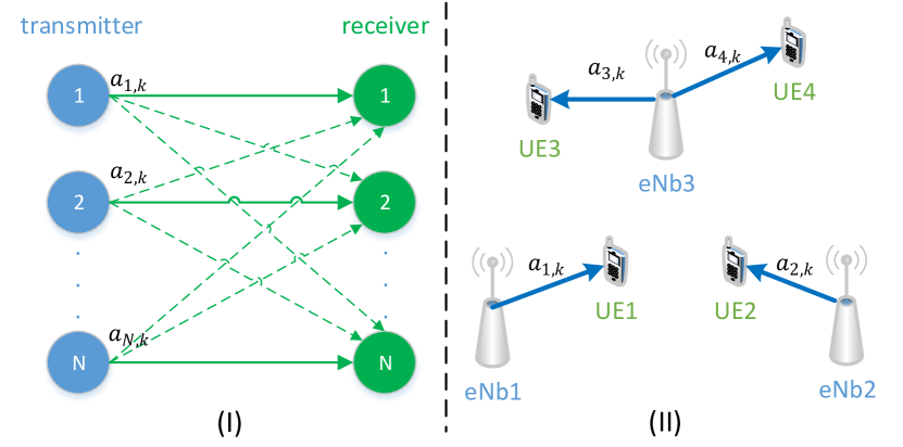
Figure 1: (I) A D2D network with $N$ transmitter-receiver pairs; (II) Downlink multi-cell network, each eNB (or base station) may serve multiple UEs (users).

This section provides some examples and shows the limit of the classical gradient-based methods.

We consider the power allocation problem in a general network with $N$ transmitter-receiver links. A link here can be seen as a node in our system model as presented in Section III. For example,

• in a D2D network with $N$ transmitter-receiver pairs, each transmitter communicates with its associated receiver and different links interfere among each other, see Figure 1 (I).

• in a multi-cell network, each base station may serve multiple users. We focus on the downlink, i.e., a user is seen as its receiver and its associated base station is seen as a transmitter, see Figure 1 (II).

In both models, the action $a_{i,k}$ is in fact the transmission power of transmitter $i$ at timeslot $k$, of which the value cannot exceed the maximum transmission power $a_{\textrm{max}}$. Thus we have $\mathcal{A}_{i}=\left[0,a_{\textrm{max}}\right]$, $\forall i\in\mathcal{N}$. The environment state matrix $\mathbf{S}_{k}$ represents the time-varying channel state of the network. More precisely, $\mathbf{S}_{k}=\left[s_{ij,k}\right]_{i\in\mathcal{N},j\in\mathcal{N}}$, in which each element $s_{ij,k}$ denotes the the channel gain between transmitter $i$ and receiver $j$ at timeslot $k$.

The utility function can be various depending on different applications, e.g., throughput and energy efficiency [27].

In our first example, the local utility of each node $i$ is given by

$$u_{i}\left(\boldsymbol{a}_{k},\mathbf{S}_{k}\right)=\omega\log\left(1+r_{i,k}\right)-\kappa a_{i,k},$$ (11)

where $\omega,\kappa\in\mathbb{R}^{+}$, $\kappa a_{i,k}$ represents the energy cost of transmission, and $r_{i,k}$ denotes the bit rate given by

$$r_{i,k}=\log\left(1+\mathtt{SINR}_{i,k}\right)\textrm{ with }\mathtt{SINR}_{i,k}=\frac{a_{i,k}s_{ii,k}}{\sigma^{2}+\sum_{j\neq i}a_{j,k}s_{ij,k}}.$$ (12)

Note that the maximization of $\log$-function of the bit rate is of type proportional fairness, which is used to ensure fairness among the nodes in the network. With the above notations, the global utility function can be written as

$$f^{\left(1\right)}\left(\boldsymbol{a}_{k},\mathbf{S}_{k}\right)=-\kappa\sum_{i\in\mathcal{N}}a_{i,k}$$

$$+\omega\sum_{i\in\mathcal{N}}\log\left(1+\log\left(1+\frac{a_{i,k}s_{ii,k}}{\sigma^{2}+\sum_{j\neq i}a_{j,k}s_{ji,k}}\right)\right).$$ (13)

It is straightforward to show that $f^{\left(1\right)}\left(\boldsymbol{a}_{k},\mathbf{S}_{k}\right)$ is concave with respect to $\boldsymbol{a}_{k}$, hence the existence of the optimum $\boldsymbol{a}^{*}$ can be guaranteed.

In order to maximize the average global utility $\mathbb{E}_{\mathbf{S}_{k}}\left(f^{\left(1\right)}\left(\boldsymbol{a}_{k},\mathbf{S}_{k}\right)\right)$, one may apply the classical stochastic approximation method described by (1). An essential step is that, each transmitter or receiver should be able to calculate the partial derivative, i.e.,

$$\widehat{g}_{i,k}=\frac{\partial f^{\left(1\right)}}{\partial a_{i,k}}=\frac{\omega\mathtt{SINR}_{i,k}}{\left(1+r_{i,k}\right)a_{i,k}}-\kappa$$

$$\quad-\sum_{n\in\mathcal{N}}\frac{\omega\mathtt{SINR}_{n,k}^{2}}{\left(1+r_{n,k}\right)\left(1+\mathtt{SINR}_{n,k}\right)}\frac{s_{ni,k}}{a_{n,k}s_{nn,k}}.$$ (14)

From (14), we find that the direct calculation of the partial derivative is complicated and nodes should exchange much information: Each node $i$ should know the values of $\mathtt{SINR}_{n,k}$, the cross-channel gain $s_{ni,k}$, as well as $a_{n,k}s_{nn,k}$ of all nodes $n\in\mathcal{N}$. Moreover, in the situation where the channel is time-varying, it is not realistic for any receiver $n$ to estimate the direct-channel gain $s_{nn,k}$ and all the cross-channel gain $s_{nj,k}$, $\forall j\in\mathcal{N}\setminus\left\{n\right\}$.

We consider the sum-rate maximization problem as a second example, i.e., to maximize $y_{k}=\sum_{i\in\mathcal{N}}r_{i,k}$. The challenge come from the fact that $y_{k}$ is not concave with respect to $a_{i,k}$ if the rate $r_{i,k}$ is given by (12). For this reason, we have to consider the approximation of $r_{i,k}$ and some variable change to make the objective function concave, which is a well known problem [28]. It is common to use change of variable (i.e., consider $\textrm{e}^{a_{i,k}}$ as the transmission power instead of $a_{i,k}$) and consider the approximation $r_{i,k}\approx\log\left(\mathtt{SINR}_{i,k}\right)$ [28], so that the global utility function is written as

$$f^{\left(2\right)}\!\left(\boldsymbol{a}_{k},\mathbf{S}_{k}\right)\!=\!\omega\!\sum_{i\in\mathcal{N}}\!\log\!\left(\!\!\frac{s_{ii,k}\textrm{e}^{a_{i,k}}}{\sigma^{2}+\sum_{j\neq i}s_{ji,k}\textrm{e}^{a_{j,k}}}\!\!\right)\!-\kappa\!\sum_{i\in\mathcal{N}}\!\textrm{e}^{a_{i,k}}.$$ (15)

It is straightforward to show the concavity of $f^{\left(2\right)}$. Similar to (14), we evaluate

$$\widehat{g}_{i,k} =\frac{\partial f^{\left(2\right)}}{\partial a_{i,k}}$$

$$=\omega-\omega\!\sum_{n\in\mathcal{N}}\!\!\frac{s_{in,k}\textrm{e}^{a_{i,k}}}{\sigma^{2}+\sum_{j\neq n}\delta_{j,k}s_{jn,k}\textrm{e}^{a_{j,k}}}\!-\kappa\!\sum_{i\in\mathcal{N}}\!\textrm{e}^{a_{i,k}},$$ (16)

of which the calculation also requires much information, such as the cross-channel gain $s_{in,k}$ $\forall n\in\mathcal{N}\setminus\left\{i\right\}$, and all the interference estimated by each receiver. All the channel information has to be estimated and exchanged by each active node, which is a huge burden for the network.

The two examples clearly shows the limit of the classical methods and motivates us to propose some novel solution where low informational exchange are required. In this paper, we consider that the nodes can only exchange their numerical approximation of local utilities. It is worth mentioning that the information exchange in our setting is much less than the gradient based method. We present our distributed optimization algorithms as well as their performance, in the situations where each node has the complete or incomplete knowledge of the local utilities of the other nodes, respectively. It is worth mentioning that, apart from the examples presented in this section, the solution proposed in this paper can also be applied to other type of problems such beamforming, coordinated multipoint (CoMP) [29], and so on.

V Distributed optimization algorithm using stochastic perturbation

This section presents a first version of our distributed optimization algorithm. We assume that each node is always able to collect the numerical estimation of local utilities from all the other nodes. In this situation, each node can evaluate the numerical value of the global utility function at each iteration (or timeslot) $k$ by applying

$$\widetilde{f}\left(\boldsymbol{a},\mathbf{S}_{k}\right) =\sum_{i\in\mathcal{N}}\widetilde{u}_{i,k}=\sum_{i\in\mathcal{N}}\left(u_{i}\left(\boldsymbol{a},\mathbf{S}_{k}\right)+\eta_{i,k}\right)$$

$$=f\left(\boldsymbol{a},\mathbf{S}_{k}\right)+\sum_{i\in\mathcal{N}}\eta_{i,k},$$ (17)

since each node knows the complete information of $\widetilde{u}_{i,k}$ for any $i\in\mathcal{N}$. We first consider an unconstrained optimization problem, i.e., $\mathcal{A}=\mathbb{R}^{N}$, in Section V-A. The constrained optimization problem with $\mathcal{A}_{i}=\left[a_{i,\min},a_{i,\max}\right]$, $\forall i\in\mathcal{N}$ is then presented in Section V-D.

V-A Algorithm

The distributed optimization algorithm using stochastic perturbation (DOSP) is presented in Algorithm 1.

Algorithm 1 DOSP Algorithm for each node $i$

1. Initialize $k=0$ and set the action $a_{i,0}$ randomly.

2. Generate a random variable $\Phi_{i,k}$, perform action $a_{i,k}+\gamma_{k}\Phi_{i,k}$.

3. Estimate $\widetilde{u}_{i,k}$, exchange its value with the other nodes and calculate $\widetilde{f}\left(\boldsymbol{a}_{k}+\gamma_{k}\boldsymbol{\Phi}_{k},\mathbf{S}_{k}\right)=\sum_{j\in\mathcal{N}}\widetilde{u}_{i,k}.$

4. Update $a_{i,k+1}$ according to equation (18).

5. $k=k+1$, go to 2.

At each iteration $k$, an arbitrary reference node $i$ updates its action by applying

$$a_{i,k+1}=a_{i,k}+\beta_{k}\Phi_{i,k}\widetilde{f}\left(\boldsymbol{a}_{k}+\gamma_{k}\boldsymbol{\Phi}_{k},\mathbf{S}_{k}\right),$$ (18)

in which $\beta_{k}$ and $\gamma_{k}$ are vanishing step-sizes, $\Phi_{i,k}$ is randomly generated by each node $i$ and $\boldsymbol{\Phi}_{k}=\left[\Phi_{1,k},\ldots,\Phi_{N,k}\right]$. Recall that the approximation $\widetilde{f}$ of the global utility is calculated by each node using (17), of which the value depends on the actual action performed by each node $\widehat{a}_{i,k}=a_{i,k}+\gamma_{k}\Phi_{i,k}$ and the environment state matrix $\mathbf{S}_{k}$. Note that $\widehat{a}_{i,k}$ is very close to $a_{i,k}$ when $k$ is large as $\gamma_{k}$ is vanishing. An example is presented in Section V-B to describe in detail the application of Algorithm 1 in practice.

Obviously, (18) can be written in the general form (1), in which

$$\widehat{g}_{i,k}=\Phi_{i,k}\widetilde{f}\left(\boldsymbol{a}_{k}+\gamma_{k}\boldsymbol{\Phi}_{k},\mathbf{S}_{k}\right).$$ (19)

As we will discuss in Section V-C, $\widehat{g}_{i,k}$ can be an asymptotically unbiased estimation of the partial derivative $\partial F/\partial a_{i}$ and $\boldsymbol{a}_{k}$ can converge to $\boldsymbol{a}^{*}$, under the condition that the parameters $\beta_{k}$, $\gamma_{k}$, and $\boldsymbol{\Phi}_{k}$ are properly chosen. We state in what follows the desirable properties of these parameters.

• A4. (properties of step-sizes) Both $\beta_{k}$ and $\gamma_{k}$ take real positive values with $\lim_{k\rightarrow\infty}\beta_{k}=\lim_{k\rightarrow\infty}\gamma_{k}=0$, besides,

  $$\sum_{k=1}^{\infty}\beta_{k}\gamma_{k}=\infty,\qquad\sum_{k=1}^{\infty}\beta_{k}^{2}<\infty.$$

• A5. (properties of random perturbation) The elements of $\boldsymbol{\Phi}_{k}$ are i.i.d. with $\mathbb{E}\left(\Phi_{i,k}\Phi_{j,k}\right)=0$, $\forall i\neq j$. There exist $\alpha_{2}>0$ and $\alpha_{3}>0$ such that

  $$\mathbb{E}\left(\Phi_{i,k}^{2}\right)=\alpha_{2},\quad\left|\Phi_{i,k}\right|\leq\alpha_{3}.$$

The conditions on the parameters can be easily achieved. We show in Example 1 a common setting of these parameters, which are also used to obtain the simulation results to be presented in Section VIII.

Example 1.

An easiest choice of the probability distribution of $\Phi_{i,k}$ is the symmetrical Bernoulli distribution with $\Phi_{i,k}\in\left\{-1,1\right\}$ and $\mathbb{P}\left(\Phi_{i,k}=1\right)=\mathbb{P}\left(\Phi_{i,k}=-1\right)=0.5$, $\forall i,k$. We can verify the conditions in A5 with $\alpha_{2}=\alpha_{3}=1$.

Let $\beta_{k}=\beta_{0}\left(k+1\right)^{-\nu_{1}}$ and $\gamma_{k}=\gamma_{0}\left(k+1\right)^{-\nu_{2}}$ with the constants $\beta_{0},\gamma_{0},\nu_{1},\nu_{2}\in\mathbb{R}^{+}$, so that both $\beta_{k}$ and $\gamma_{k}$ are vanishing. Since $\sum_{k=1}^{\infty}\beta_{k}^{2}$ converges if $\nu_{1}>0.5$; $\sum_{k=1}^{\infty}\beta_{k}\gamma_{k}$ diverges if $\nu_{1}+\nu_{2}\leq 1$. Clearly, there exist pairs of $\nu_{1}$ and $\nu_{2}$ to make $\beta_{k}$ and $\gamma_{k}$ satisfy the conditions in A4.

Remark 1.

The proposed algorithm has similar shape compared with the other existed methods proposed in [26, 24, 25]. The difference between our solution and the sine perturbation based method [24, 25] is that, we use a random vector $\boldsymbol{\Phi}_{k}$ instead of some deterministic sine functions as the perturbation term. Comparing (4) and (18), we can see that the amplitude of random perturbation is vanishing in our algorithm, which is not the case in the algorithm presented in [26].

V-B Application example

This section presents the application of Algorithm 1 to perform resource allocation in a D2D network, in order to highlight the interest of our solution. We focus on the requirement arisen by Algorithm 1, in terms of computation, memory and informational exchange.

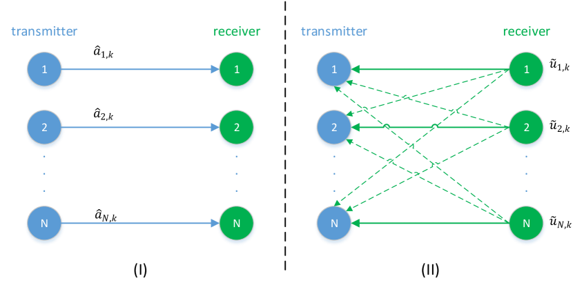
Figure 2: (I) At iteration $k$, each transmitter $i$ transmits to its associated receiver with transmission power $\widehat{a}_{i,k}$; (II) Each receiver $i$ sends the approximate local utility $\widetilde{u}_{i,k}$ to its transmitter, every transmitter can receive and decode this feedback information.

Figure 2 briefly shows the algorithm procedure during one iteration. Recall that $\widehat{a}_{i,k}$ denotes the actual value of the action set by transmitter $i$ at iteration $k$. In order to update $\widehat{a}_{i,k}$, each transmitter $i$ needs to

• independently and randomly generate a scalar $\Phi_{i,k}$ under the condition A5;

• use a pre-defined vanishing sequence $\gamma_{k}$ which is common for each link;

• independently update $a_{i,k}$ by applying (18), more details will be provided soon.

Then $\widehat{a}_{i,k}$ is given by $\widehat{a}_{i,k}=a_{i,k}+\gamma_{k}\Phi_{i,k}$.

Each transmitter $i$ transmits to its associated receiver with the transmission power of value $\widehat{a}_{i,k}$. The associated receiver $i$ should be able to approximate the numerical value of its local utility $\widetilde{u}_{i,k}$ and send this value to transmitter $i$ as a feedback. All the transmitters can evaluate $\widetilde{f}\left(\widehat{\boldsymbol{a}}_{k}\right)$ using (17) under the assumption that every transmitter is able to receive and decode the feedback from all the receivers.

Then iteration $k+1$ starts, each transmitter $i$ needs to update its power allocation strategy, what is required is listed as follows:

• use a pre-defined vanishing sequence $\beta_{k}$;

• reuse of the local random value $\Phi_{i,k}$, which was generated by transmitter $i$ at iteration $k$. It means that the value of $\Phi_{i,k}$ should be saved temporarily

• use the numerical value of $\widetilde{f}_{k}\left(\widehat{\boldsymbol{a}}_{k}\right)$, which has been explained already.

Each transmitter can then update $a_{i,k+1}$ independently using (18).

In the following step, each transmitter updates $\widehat{a}_{i,k+1}$ in the same way as the previous iteration, i.e., $\widehat{a}_{i,k+1}=a_{i,k+1}+\gamma_{k+1}\Phi_{i,k+1},$ with $\Phi_{i,k+1}$ a newly generated pseudo-random value.

We can see that Algorithm 1 can be easily applied in a network of multiple links: the algorithm itself has low complexity and each receiver only needs to feedback one quantity ($\widetilde{u}_{i,k}$) per iteration to perform the algorithm.

V-C Convergence results

This section investigates the asymptotic behavior of Algorithm 1. For any integer $k\geq 0$, we consider the divergence

$$d_{k}=\left\|\boldsymbol{a}_{k}-\boldsymbol{a}^{*}\right\|^{2}$$ (20)

to describe the difference between the actual action $\boldsymbol{a}_{k}$ and the optimal action $\boldsymbol{a}^{*}$. Our aim is to show that $d_{k}\rightarrow 0$ almost surely as $k\rightarrow\infty$.

In order to explain the reason behind the update rule (18), we rewrite it in the generalized Robbins-Monro form [20], i.e.,

$$\boldsymbol{a}_{k+1}=\boldsymbol{a}_{k}+\beta_{k}\widehat{\boldsymbol{g}}_{k}$$

$$=\boldsymbol{a}_{k}+\beta_{k}\left(\alpha_{2}\gamma_{k}\nabla F\left(\boldsymbol{a}_{k}\right)+\overline{\boldsymbol{g}}_{k}-\alpha_{2}\gamma_{k}\nabla F\left(\boldsymbol{a}_{k}\right)+\widehat{\boldsymbol{g}}_{k}-\overline{\boldsymbol{g}}_{k}\right)$$

$$=\boldsymbol{a}_{k}+\alpha_{2}\beta_{k}\gamma_{k}\left(\nabla F\left(\boldsymbol{a}_{k}\right)+\boldsymbol{b}_{k}+\frac{\boldsymbol{e}_{k}}{\alpha_{2}\gamma_{k}}\right),$$ (21)

where $\overline{\boldsymbol{g}}_{k}$ represents the expected value of $\widehat{\boldsymbol{g}}_{k}$ with respect to all the stochastic terms (including $\boldsymbol{\Phi}$, $\mathbf{S}$, and $\boldsymbol{\eta}$) for a given $\boldsymbol{a}_{k}$, i.e.,

$$\overline{\boldsymbol{g}}_{k}=\mathbb{E}_{\mathbf{S},\boldsymbol{\Phi},\boldsymbol{\eta}}\left(\widehat{\boldsymbol{g}}_{k}\right),$$ (22)

note that we prefer to highlight the stochastic terms in (22), an alternative way is to write (22) as $\overline{\boldsymbol{g}}_{k}=\mathbb{E}\left(\widehat{\boldsymbol{g}}_{k}\mid\boldsymbol{a}_{k}\right)$; $\boldsymbol{b}_{k}$ denotes the estimation bias between $\overline{\boldsymbol{g}}_{k}$ and the actual gradient of the average objective function $F$, i.e.,

$$\boldsymbol{b}_{k} =\frac{\overline{\boldsymbol{g}}_{k}}{\alpha_{2}\gamma_{k}}-\nabla F\left(\boldsymbol{a}_{k}\right);$$ (23)

and $\boldsymbol{e}_{k}$ can be seen as the stochastic noise, which is the difference between the value of a single realization of $\widehat{\boldsymbol{g}}_{k}$ and its average $\overline{\boldsymbol{g}}_{k}$ as defined in (22), i.e.,

$$\boldsymbol{e}_{k}=\widehat{\boldsymbol{g}}_{k}-\overline{\boldsymbol{g}}_{k}.$$ (24)

Remark 2.

The analysis presented in this work is challenging and different from the existed results. An explicit difference comes from the unique feature of the algorithm itself as discussed in Remark 1: we are using a different method to estimate the gradient. Besides, the objective function is stochastic with general form in our problem, while it is considered as static in [22, 23] and it is assumed to be static and quadratic in [26].

To perform the analysis of convergence, we have to investigate the properties of $\boldsymbol{b}_{k}$ and $\boldsymbol{e}_{k}$.

Lemma 1.

If all the conditions in A1-A5 are satisfied, then

$$\left\|\boldsymbol{b}_{k}\right\|\leq\gamma_{k}N^{\frac{5}{2}}\frac{\alpha_{3}^{3}\alpha_{1}}{2\alpha_{2}}=O\left(\gamma_{k}\right),$$ (25)

which implies that $\left\|\boldsymbol{b}_{k}\right\|\rightarrow 0$ as $k\rightarrow\infty$.

Proof:

See Appendix -A. ∎

Lemma 1 implies that $\widehat{\boldsymbol{g}}_{k}$ defined in Algorithm 1 is a reasonable estimator of the gradient with vanishing bias.

Lemma 2.

If all the conditions in A1-A5 are satisfied and $\left\|\boldsymbol{a}_{k}\right\|<\infty$ almost surely, then for any constant $\rho>0$, we have

$$\lim_{K\rightarrow\infty}\mathbb{P}\left(\sup_{K^{\prime}\geq K}\left\|\sum_{k=K}^{K^{\prime}}\beta_{k}\boldsymbol{e}_{k}\right\|\geq\rho\right)=0,\quad\forall\rho>0.$$ (26)

Proof:

See Appendix -B. ∎

Based on the results in Lemma 1 and in Lemma 2, we can build conditions under which $\boldsymbol{a}_{k}\rightarrow\boldsymbol{a}^{*}$ almost surely.

Theorem 1.

If all the conditions in A1-A5 are satisfied and $\left\|\boldsymbol{a}_{k}\right\|<\infty$ almost surely, then $\boldsymbol{a}_{k}\rightarrow\boldsymbol{a}^{*}$ as $k\rightarrow\infty$ almost surely by applying Algorithm 1.

Proof:

See Appendix -C. ∎

V-D Distributed optimization under constraints

In this section, we consider the constrained optimization problem, in which the action of each node takes value from an interval, i.e., $\mathcal{A}_{i}=\left[a_{i,\min},a_{i,\max}\right]$, $\forall i\in\mathcal{N}$. We assume that $\boldsymbol{a}^{*}$ is not on the boundary of the feasible set $\mathcal{A}$, i.e., $a_{i}^{*}\in\left(a_{i,\min},a_{i,\max}\right)$, $\forall i\in\mathcal{N}$. For example, in the power allocation problem, $a_{i,k}$ presents the transmission power of transmitter $i$, which should be positive and not larger than a maximum value.

Recall that the actually performed action by nodes is $\widehat{\boldsymbol{a}}_{k}=\boldsymbol{a}_{k}+\gamma_{k}\boldsymbol{\Phi}_{k}$. At each iteration, we need to ensure that $\widehat{a}_{i,k}\in\left[a_{i,\min},a_{i,\max}\right]$. A direct solution is to introduce a projection to the algorithm, i.e., (18) turns to

$$\boldsymbol{a}_{k+1}=\mathtt{Proj}\left(\boldsymbol{a}_{k}+\beta_{k}\widehat{\boldsymbol{g}}_{k}\right),$$ (27)

in which for any $i\in\mathcal{N}$,

$$a_{i,k+1} =\min\left\{\max\left\{a_{i,k}+\beta_{k}\widehat{g}_{i,k},a_{i,\min}+\alpha_{3}\gamma_{k+1}\right\},\right.$$

$$\qquad\qquad\qquad\left.a_{i,\max}-\alpha_{3}\gamma_{k+1}\right\}.$$ (28)

As $\left|\Phi_{i,k}\right|\leq\alpha_{3}$ by A5, (28) leads to $a_{i,k+1}+\gamma_{k+1}\left|\Phi_{i,k+1}\right|\in\left[a_{i,\min},a_{i,\max}\right]$.

Remark 3.

In order to write (28) into the form similar to (21), one has to re-define the bias term $b_{i,k}$ and the stochastic noise $e_{i,k}$ because of the operator $\mathtt{Proj}$. Therefore, it is not straightforward to deduce of the convergence of the constrained optimization algorithm from the results presented in Section V-C.

Theorem 2.

In the constrained optimization problem where $\mathcal{A}_{i}=\left[a_{i,\min},a_{i,\max}\right]$ and $a_{i}^{*}\in\left(a_{i,\min},a_{i,\max}\right)$, $\forall i\in\mathcal{N}$, by applying the projection (27), we have $\boldsymbol{a}_{k}\rightarrow\boldsymbol{a}^{*}$ as $k\rightarrow\infty$ almost surely under the assumptions A1-A5.

Proof:

See Appendix -D. ∎

VI Optimization Algorithm with incomplete information of utilities of other nodes

A limit of Algorithm 1 is that each node is required to know the local utility of all the other nodes. Such issue is significant as there are many nodes in the network. It is thus important to consider a more realistic situation where a node only has has the knowledge of the local utilities of a subset $\mathcal{I}_{i,k}$ of nodes, with $\mathcal{I}_{i,k}\subseteq\mathcal{N}\setminus\left\{i\right\}$. Throughout this section, we have the following assumption:

• A6). at any iteration $k$, an arbitrary node $i$ knows the utility $\widetilde{u}_{j,k}$ of another node $j$ with a constant probability $p\in\left(0,1\right]$, $i.e.$, the elements contained in the set $\mathcal{I}_{i,k}$ is random, for any $j\neq i$, we have

  $$\mathbb{P}\left(j\in\mathcal{I}_{i,k}\right)=p,\qquad\mathbb{P}\left(j\notin\mathcal{I}_{i,k}\right)=1-p.$$ (29)

Notice that we do not assume any specified network topology and each node $i$ has a different and independent set $\mathcal{I}_{i,k}$.

We propose a modified algorithm and then show its asymptotic performance. The algorithm is described in Algorithm 2. The main difference between Algorithm 1 and Algorithm 2 comes from the approximation of the objective function, i.e.,

$$\widetilde{f}_{i}^{(\textrm{I})}\left(\boldsymbol{a},\mathbf{S}_{k},\mathcal{I}_{i,k}\right)$$

$$=\begin{cases}\widetilde{u}_{i,k}+\frac{N-1}{\left|\mathcal{I}_{i,k}\right|}\sum_{j\in\mathcal{I}_{i,k}}\widetilde{u}_{j,k},&\textrm{if }\left|\mathcal{I}_{i,k}\right|\neq 0,\\ 0,&\textrm{if }\left|\mathcal{I}_{i,k}\right|=0.\end{cases}$$ (30)

Similar to (18), the algorithm is given by

$$a_{i,k+1} =a_{i,k}+\beta_{k}\widehat{g}_{i,k}^{\left(\textrm{I}\right)}=a_{i,k}+\beta_{k}\Phi_{i,k}\widetilde{f}_{i}^{(\textrm{I})}\left(\boldsymbol{a},\mathbf{S}_{k},\mathcal{I}_{i,k}\right)$$ (31)

The basic idea is to consider $\left(N-1\right)\sum_{j\in\mathcal{I}_{i,k}}\widetilde{u}_{j,k}/\left|\mathcal{I}_{i,k}\right|$ as a surrogate function of $\sum_{j\in\mathcal{N}\setminus\left\{i\right\}}\widetilde{u}_{j,k}$, in the case where the set $\mathcal{I}_{i,k}$ is non-empty. Otherwise, node $i$ does not know any utility of the other nodes, it then cannot estimate the global utility of the system. As a result, node $i$ keeps its previous action, i.e., $a_{i,k+1}=a_{i,k}$. Note that different users may have different knowledge of the global utility as $\mathcal{I}_{i,k}$ is independent for each node $i$. For example, node $i$ may know $\widetilde{u}_{j,k}$ of a different node $j$, whereas node $j$ may not know $\widetilde{u}_{i,k}$.

Algorithm 2 DOSP algorithm for each node $i$ with incomplete information of the utilities of other nodes

1. Initialize $k=0$ and set the action $a_{i,0}$ randomly.

2. Generate a random variable $\Phi_{i,k}$, perform action $a_{i,k}+\gamma_{k}\Phi_{i,k}$.

3. Estimate $\widetilde{u}_{i,k}$, exchange its value with the other nodes and calculate $\widetilde{f}_{i}^{(\textrm{I})}$ using (30) based on the collected local utilities.

4. Update $a_{i,k+1}$ according to equation (31).

5. $k=k+1$, go to 2.

Due to the additional random term $\mathcal{I}_{i,k}$, the convergence analysis of Algorithm 2 is more complicated than that of Algorithm 1. We start with Lemma 3, which is useful for the analysis in what follows

Lemma 3.

The expected value of $\widetilde{f}_{i}^{(\textrm{I})}\left(\boldsymbol{a},\mathbf{S}_{k},\mathcal{I}_{i,k}\right)$ over all possible sets $\mathcal{I}_{i,k}$ is proportional to $\widetilde{f}\left(\boldsymbol{a},\mathbf{S}_{k}\right)$, i.e.,

$$\mathbb{E}_{\mathcal{I}_{i,k}}\left(\widetilde{f}_{i}^{(\textrm{I})}\left(\boldsymbol{a},\mathbf{S}_{k},\mathcal{I}_{i,k}\right)\right)=(1-(1-p)^{N})\widetilde{f}\left(\boldsymbol{a},\mathbf{S}_{k}\right).$$ (32)

Proof:

See Appendix -E. ∎

To simplify the notation, introduce

$$q=\mathbb{P}\left(\left|\mathcal{I}_{i,k}\right|\neq 0\right)=1-(1-p)^{N}.$$ (33)

Similar to (21), we rewrite (31) as

$$a_{i,k+1} =a_{i,k}+\alpha_{2}q\beta_{k}\gamma_{k}\left(F_{i}^{\prime}\left(\boldsymbol{a}_{k}\right)+b_{i,k}^{\left(\textrm{I}\right)}+\frac{e_{i,k}^{\left(\textrm{I}\right)}}{\alpha_{2}q\gamma_{k}}\right)$$ (34)

with

$$b_{i,k}^{\left(\textrm{I}\right)} =\frac{\mathbb{E}_{\mathbf{S},\boldsymbol{\Phi},\boldsymbol{\eta},\mathcal{I}_{i,k}}\left(\widehat{g}_{i,k}^{(\textrm{I})}\right)}{\alpha_{2}q\gamma_{k}}-F_{i}^{\prime}\left(\boldsymbol{a}_{k}\right),$$ (35)

$$e_{i,k}^{\left(\textrm{I}\right)} =\widehat{g}_{i,k}^{\left(\textrm{I}\right)}-\mathbb{E}_{\mathbf{S},\boldsymbol{\Phi},\boldsymbol{\eta},\mathcal{I}_{i,k}}\left(\widehat{\boldsymbol{g}}_{k}^{(\textrm{I})}\right).$$ (36)

We need to investigate the property of $b_{i,k}^{\left(\textrm{I}\right)}$ and $e_{i,k}^{\left(\textrm{I}\right)}$ in order to show the convergence of Algorithm 2. The proof is more complicated because of the additional random term $\mathcal{I}_{i,k}$ in both $b_{i,k}^{\left(\textrm{I}\right)}$ and $e_{i,k}^{\left(\textrm{I}\right)}$ compared with $b_{i,k}$ and $e_{i,k}$ discussed in Section V.

Theorem 3.

In the situation where nodes do not have the access to all the other nodes’ local utilities and the objective function is approximated by applying (30), then we still have $\boldsymbol{a}_{k}\rightarrow\boldsymbol{a}^{*}$ as $k\rightarrow\infty$ almost surely by applying Algorithm 2, as long as the assumptions A1-A6 hold and $\left\|\boldsymbol{a}_{k}\right\|<\infty$ almost surely.

Proof:

See Appendix -F. ∎

Remark 4.

Although the asymptotic convergence still holds, the convergence speed is reduced if the information of the objective function is incomplete. By comparing (21) and (34), we can see that the equivalent step size is decreased by $q$ times. Moreover, the variance of the stochastic noise $e_{i,k}^{\left(\textrm{I}\right)}$ is higher, as the randomness is more significant when we use $n<N$ random symbols to represent the average of $N$ symbols. More discussion related to the convergence rate will be provided in Section VII.

VII Convergence rate

In this section, we study the average convergence rate of the proposed algorithm in order to investigate how fast the proposed algorithms converge to the optimum from a quantitative point of view. The analysis also provides a detailed guideline of setting the parameters $\beta_{k}$ and $\gamma_{k}$ which determine the convergence rate. We start with the analysis considering general forms of $\beta_{k}$ and $\gamma_{k}$. A widely used example is then considered afterwards.

VII-A General analysis

As a common setting in the analysis of the convergence rate [30], we have an additional assumption on the concavity of the objective function in this section, i.e.,

• A7. $F\left(\boldsymbol{a}\right)$ is strongly concave, there exists $\alpha_{5}>0$ such that

  $$\left(\boldsymbol{a}-\boldsymbol{a}^{*}\right)^{T}\nabla F\left(\boldsymbol{a}_{k}\right)\leq-\alpha_{5}\left\|\boldsymbol{a}-\boldsymbol{a}^{*}\right\|_{2}^{2},\quad\forall\boldsymbol{a}\in\mathcal{A}.$$ (37)

In this section, we are interested in the evolution of the average divergence $D_{k}=\mathbb{E}(\left\|\boldsymbol{a}_{k}-\boldsymbol{a}^{*}\right\|_{2}^{2}$). In order to distinguish the two versions of algorithms with complete and incomplete information of local utilities, we use $D_{k}^{\left(\textrm{C}\right)}$ and $D_{k}^{\left(\textrm{I}\right)}$ to denote the divergence resulted by Algorithm 1 and Algorithm 2, respectively.

An essential step of the analysis of the convergence rate is to investigate the relation of the divergence between two successive iterations.

Denote $M^{\left(\mathrm{C}\right)}$ and $M^{\left(\mathrm{I}\right)}$ as the upper bounds of $\mathbb{E}(\left\|\widehat{\boldsymbol{g}}_{k}\right\|_{2}^{2})$ and of $\mathbb{E}(\left\|\widehat{\boldsymbol{g}}_{k}^{\left(\mathrm{I}\right)}\right\|_{2}^{2})$ in Algorithm 1 and Algorithm 2 respectively. Our result is stated in Lemma (4).

Lemma 4.

Assume that A7 holds, for any $k\geq 1$, $D_{k}^{\left(\mathrm{C}\right)}$ resulted by Algorithm 1 is such that

$$D_{k+1}^{\left(\mathrm{C}\right)}\leq\left(1-2\alpha_{2}\alpha_{5}\beta_{k}\gamma_{k}\right)D_{k}^{\left(\mathrm{C}\right)}$$

$$\qquad\qquad\qquad+N^{\frac{5}{2}}\alpha_{1}\alpha_{3}^{3}\beta_{k}\gamma_{k}^{2}\sqrt{D_{k}^{\left(\mathrm{C}\right)}}+M^{\left(\mathrm{C}\right)}\beta_{k}^{2},$$ (38)

Similarly, $D_{k}^{\left(\mathrm{I}\right)}$ resulted by Algorithm 2 is such that

$$D_{k+1}^{\left(\mathrm{I}\right)}\leq\left(1-2\alpha_{2}\alpha_{5}q\beta_{k}\gamma_{k}\right)D_{k}^{\left(\mathrm{I}\right)}$$

$$\qquad\qquad\qquad+N^{\frac{5}{2}}\alpha_{1}\alpha_{3}^{3}q\beta_{k}\gamma_{k}^{2}\sqrt{D_{k}^{\left(\mathrm{I}\right)}}+M^{\left(\mathrm{I}\right)}\beta_{k}^{2}.$$ (39)

Proof:

See Appendix -G. ∎

We can see that both (38) and (39) can be written in the simplified general form

$$D_{k+1}\leq\left(1-A\beta_{k}\gamma_{k}\right)D_{k}+B\beta_{k}\gamma_{k}^{2}\sqrt{D_{k}}+C\beta_{k}^{2},$$ (40)

with positive constants

$$A^{\left(\mathrm{C}\right)}=2\alpha_{2}\alpha_{5},\>B^{\left(\mathrm{C}\right)}=N^{\frac{5}{2}}\alpha_{1}\alpha_{3}^{3},\>C^{\left(\mathrm{C}\right)}=M^{\left(\mathrm{C}\right)}$$ (41)

in (38) and

$$A^{\left(\mathrm{I}\right)}=2q\alpha_{2}\alpha_{5},\>B^{\left(\mathrm{I}\right)}=qN^{\frac{5}{2}}\alpha_{1}\alpha_{3}^{3},\>C^{\left(\mathrm{I}\right)}=M^{\left(\mathrm{I}\right)}$$ (42)

in (39).

Remark 5.

In the constrained optimization problem, we can obtain the same result as Lemma 4 directly from (68), for any $k\geq K_{\mathrm{c}}$. In fact, the unconstrained optimization problem can be seen as a special case of the constrained optimization problem with $a_{i,\min}=-\infty$, $a_{i,\max}=+\infty$, and $K_{\mathrm{c}}=0$. For this reason, we consider the general problem with $K_{\mathrm{c}}$ taken into account, in the rest of this section.

Introduce

$$K_{0}=\underset{k\geq K_{\mathrm{c}},\beta_{k}\gamma_{k}<1/A}{\arg\min}k,$$

which implies that $1-A\beta_{k}\gamma_{k}>0$ and $k\geq K_{\mathrm{c}}$ as $k\geq K_{0}$.

Lemma 4 provides us the relation between $D_{k+1}$ and $D_{k}$. Our next goal is to search a vanishing upper bound of $D_{k}$ using (40). In other words, we aim to search a sequence $U_{K_{0}},\ldots,U_{k},\ldots$ such that

$$U_{k+1}\leq U_{k}\textrm{ and }D_{k}\leq U_{k},\>\forall k\geq K_{0}.$$

This type of analysis is usually performed by induction: consider a given expression of $U_{k}$ and assume that $D_{k}\leq U_{k}$, one needs to show that $D_{k+1}\leq U_{k+1}$ by applying (40).

An important issue is then the proper choice of the form of the upper bound $U_{k}$. Note that there exists only one step-size $\beta_{k}$ in the classical stochastic approximation algorithm described by (1), it is relatively simple to determine the form of $U_{k}$ with a further setting $\beta_{k}=\beta_{0}k^{-1}$, see [30]. Our problem is much more complicated as we use two step-sizes $\beta_{k}$ and $\gamma_{k}$ with general form under Assumption A4. The following lemma presents an important property of $U_{k}$.

Lemma 5.

If there exists a decreasing sequence $U_{K_{0}},\ldots,U_{k},\ldots$ such that $D_{k+1}\leq U_{k+1}$ can be deduced from $D_{k}\leq U_{k}$ and (40), then ,

$$U_{k}\geq\left(\frac{B}{2A}\gamma_{k}+\sqrt{\left(\frac{B}{2A}\right)^{2}\gamma_{k}^{2}+\frac{C}{A}\frac{\beta_{k}}{\gamma_{k}}}\right)^{2}.$$ (43)

Proof:

See Appendix -H. ∎

Note that the lower bound of $U_{k}$ is vanishing as $\gamma_{k}\rightarrow 0$ and $\beta_{k}/\gamma_{k}\rightarrow 0$. Such bound means that, using induction by developing (40), the convergence rate of $D_{k}$ cannot be better than the decreasing speed of $\gamma_{k}^{2}$ and of $\beta_{k}/\gamma_{k}$. After the verification of the existence of bounded constant $\vartheta$ or $\varrho$ such that $D_{k}\leq\vartheta^{2}\gamma_{k}^{2}$ or $D_{k}\leq\varrho^{2}\gamma_{k}/\beta_{k}$, we obtain the final results stated as follows.

Theorem 4.

Define the following parameters:

$$\chi_{k}=\frac{1-\left(\frac{\gamma_{k+1}}{\gamma_{k}}\right)^{2}}{\beta_{k}\gamma_{k}},\epsilon_{1}=\max_{k\geq K_{0}}\chi_{k},\epsilon_{2}=\max_{k\geq K_{0}}\frac{\beta_{k}}{\gamma_{k}^{3}},$$ (44)

$$\varpi_{k}=\frac{1-\frac{\beta_{k+1}\gamma_{k+1}^{-1}}{\beta_{k}\gamma_{k}^{-1}}}{\beta_{k}\gamma_{k}},\epsilon_{3}=\max_{k\geq K_{0}}\varpi_{k},\epsilon_{4}=\max_{k\geq K_{0}}\sqrt{\frac{\gamma_{k}^{3}}{\beta_{k}}}$$ (45)

If $\chi_{k}<A$ for any $k\geq K_{0}$, then

$$D_{k}\leq\vartheta^{2}\gamma_{k}^{2},\>\forall k\geq K_{0},$$ (46)

with

$$\vartheta\geq\max\left\{\frac{\sqrt{D_{K_{0}}}}{\gamma_{K_{0}}},\frac{B+\sqrt{B^{2}+4C\epsilon_{2}\left(A-\epsilon_{1}\right)}}{2\left(A-\epsilon_{1}\right)}\right\},$$ (47)

If $\varpi_{k}<A$ for any $k\geq K_{0}$, then

$$D_{k}\leq\varrho^{2}\frac{\beta_{k}}{\gamma_{k}},\>\forall k\geq K_{0},$$ (48)

with

$$\varrho\geq\max\left\{\sqrt{\frac{D_{K_{0}}\gamma_{K_{0}}}{\beta_{K_{0}}}},\frac{B\epsilon_{4}+\sqrt{\left(B\epsilon_{4}\right)^{2}+4C\left(A-\epsilon_{3}\right)}}{2\left(A-\epsilon_{3}\right)}\right\}.$$ (49)

Proof:

See Appendix -I. ∎

For general forms of $\beta_{k}$ and $\gamma_{k}$, Theorem 4 provides two upper bounds of the average divergence $D_{k}^{\left(\textrm{C}\right)}$ and $D_{k}^{\left(\textrm{I}\right)}$. The conditions that $\chi_{k}<A$ and $\varpi_{k}<A$ can be checked easily considering any fixed $\beta_{k}$ and $\gamma_{k}$. In the situation where both conditions are satisfied, we have

$$D_{k}\leq\min\left\{\vartheta^{2}\gamma_{k}^{2},\varrho^{2}\frac{\beta_{k}}{\gamma_{k}}\right\},\>\forall k\geq K_{0}.$$

From Theorem 4, we can see that the decreasing order of $D_{k}^{\left(\textrm{C}\right)}$ and $D_{k}^{\left(\textrm{I}\right)}$ mainly depend on the step-sizes $\beta_{k}$ and $\gamma_{k}$, the incompleteness factor $q$ only has the influence on the constant terms $\vartheta$ and $\varrho$, which are functions of the parameters $A$, $B$, and $C$ defined in (41) and (42). The results of convergence rate are useful to properly choose the parameters of the algorithm. Intuitively, we need to make $\gamma_{k}^{2}$ or $\beta_{k}/\gamma_{k}$ decrease as fast as possible, having the constant $\epsilon_{1}$, $\epsilon_{2}$, $\epsilon_{3}$, and $\epsilon_{4}$ as small as possible.

VII-B A special case

In this section, we consider an example as mentioned in Example 1:

$$\beta_{k}=\beta_{0}\left(k+1\right)^{-\nu_{1}}\textrm{ and }\gamma_{k}=\gamma_{0}\left(k+1\right)^{-\nu_{2}}.$$ (50)

Recall that $0.5<\nu_{1}<1$ and $0<\nu_{2}\leq 1-\nu_{1}$ in order to meet the conditions in A4.

Theorem 5.

Consider $\beta_{k}$ and $\gamma_{k}$ with given forms (50), if $\beta_{0}\gamma_{0}\geq\max\left\{2\nu_{2},\nu_{1}-\nu_{2}\right\}/A$, then there exists $\Omega<\infty$, such that

$$D_{k}\leq\Omega\left(k+1\right)^{-\min\left\{2\nu_{2},\nu_{1}-\nu_{2}\right\}},\quad\forall k\geq K_{0}.$$ (51)

Proof:

See Appendix -J. ∎

We can see the explicit impact of each parameter on the upper bound of the convergence rate from Theorem 5. It is easy to show that

$$\max\left\{2\nu_{2},\nu_{1}-\nu_{2}\right\}\leq 0.5$$

with the equality holds when $\nu_{1}=0.75$ and $\nu_{2}=0.25$, which corresponds to the best choice of $\nu_{1}$ and $\nu_{2}$ to optimize the decreasing order of the upper bound of $D_{k}$. Theorem 5 also provides a sufficient condition on the parameters that should be satisfied in order to ensure the validation of the convergence rate.

In what follows, we present a toy example to verify Theorem  5.

Example 2.

Consider $N=2$ and a simple quadratic function $f\left(\boldsymbol{a},\mathbf{S}\right)=-s_{1}a_{1}^{2}-s_{2}a_{2}^{2}+a_{1}a_{2}+a_{1}+a_{2}$ with $a_{1},a_{2}\in\left[0,3\right]$. Both $s_{1}$ and $s_{2}$ are realizations of a uniform distributed random variable $S$ which takes value from an interval $[0.5,1.5]$. Taking the average, the objective function is

$$F\left(\boldsymbol{a}\right)=-a_{1}^{2}-a_{2}^{2}+a_{1}a_{2}+a_{1}+a_{2}.$$

It is straightforward to get that $F\left(\boldsymbol{a}\right)$ takes its maximum value when $a_{1}=a_{2}=1$. We can also deduce that $F$ is strongly concave with $\alpha_{5}=1$ in (37). We set the perturbation $\boldsymbol{\Phi}_{k}$ as introduced in Example 1, with $\alpha_{2}=1$. Thus we have $A=2\alpha_{2}\alpha_{5}=2$ by (41). Let $\beta_{k}=\beta_{0}\left(k+1\right)^{-0.75}$ and $\gamma_{k}=\left(k+1\right)^{-0.25}$.

By setting $\beta_{0}\in\left\{0.23,0.28,0.5\right\}$, we can verify the importance of the condition $\beta_{0}\gamma_{0}\geq 0.25=\max\left\{2\nu_{2},\nu_{1}-\nu_{2}\right\}/A$ as presented in Theorem 5. Figure 3 shows the comparison results between the divergence $D_{k}$ averaged by 1000 simulations and the bound $\Omega\left(k+1\right)^{-0.5}$ from (51). Note that we are mainly interested in the asymptotic decreasing order of $D_{k}$, thus we set the constant term $\Omega=2$ mainly to facilitate the visual comparison of different curves. We find that the curves of $D_{k}$ decrease not-less-slowly than the bound as $\beta_{0}\in\left\{0.28,0.5\right\}$. When $\beta_{0}=0.23<0.25$, the convergence rate cannot be guaranteed, which further justify our claim in Theorem 5.

Now we fix the values of $\beta_{0}$ and $\gamma_{0}$ and consider $\left(\nu_{1},\nu_{2}\right)\in\{\left(0.55,0.15\right),\left(0.7,0.15\right),\left(0.5,0.2\right),\left(0.65,0.35\right)\}$. Notice that all the four pairs of $\left(\nu_{1},\nu_{2}\right)$ lead to the same decreasing order of the upper bound (51), as $\min\left\{2\nu_{2},\nu_{1}-\nu_{2}\right\}=0.3$. The curves of $D_{k}$ (averaged by 2000 simulations) are compared with the upper bound $\Omega\left(k+1\right)^{-0.3}$ in Figure 4. Clearly, when the number of iterations is large enough, all the curves decrease with the same speed or even faster, compared with the bound.

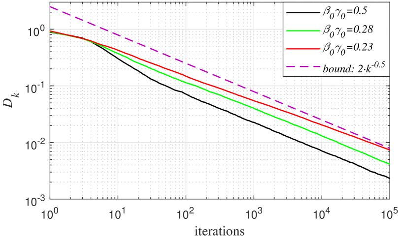
Figure 3: Comparison of the theoretical upper bound $2\left(k+1\right)^{-0.5}$ with the evolution of the average divergence $D_{k}$ (by 2000 simulations) using $\beta_{k}=\beta_{0}\left(k+1\right)^{0.75}$ and $\gamma_{k}=\left(k+1\right)^{0.25}$, with $\beta_{0}\in\left\{0.23,0.28,0.5\right\}$.

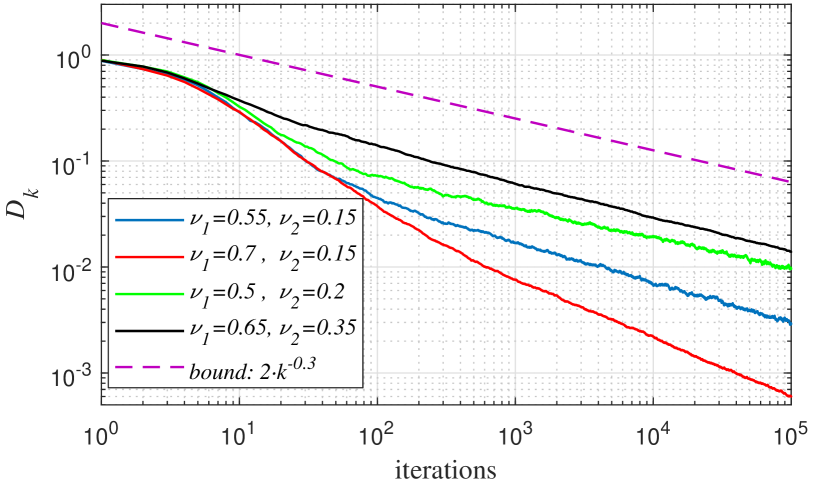
Figure 4: Comparison of the theoretical upper bound $2\left(k+1\right)^{-0.3}$ with the evolution of the average divergence $D_{k}$ (by 2000 simulations) using $\beta_{k}=0.4\cdot\left(k+1\right)^{\nu_{1}}$ and $\gamma_{k}=\left(k+1\right)^{\nu_{2}}$, with $\left(\nu_{1},\nu_{2}\right)\in\left\{\left(0.55,0.15\right),\left(0.7,0.15\right),\left(0.5,0.2\right),\left(0.65,0.35\right)\right\}$

VIII Simulation Results

In this section, we apply our algorithm to a power control problem as introduced in Section IV in order to have some numerical results. We consider (13) as the local utility function of each node. The time varying channel $h_{ij}$ between node $i$ (transmitter) and node $j$ (receiver) is generated using a Gaussian distribution with variance $\sigma_{ii}^{2}=1$ and $\sigma_{ij}^{2}=0.1$, $\forall i\neq j$. Notice that the channel gain is $s_{ij}=\left|h_{ij}\right|^{2}$. Besides, we set $\sigma^{2}=0.2$, $\omega=20$ and $\kappa=1$.

VIII-A Simulations with 4 nodes

In this section, we consider $N=4$ nodes. In all the simulations (applying different algorithms), the step size follows $\beta_{k}=2.5k^{-0.75}$, and the initial values of $a_{0,i}$ ($\forall i\in\mathcal{N}$) are generated uniformly in the interval $\left(0,20\right]$. In both Algorithm 1 and Algorithm 2, $\gamma_{k}=12k^{-0.25}$ and $\Phi_{i,k}$ follows the symmetrical Bernoulli distribution, i.e., $\mathbb{P}\left(\Phi_{i,k}=1\right)=\mathbb{P}\left(\Phi_{i,k}=-1\right)=0.5$, $\forall k,i$.

We first compare our proposed algorithm with the sine perturbation based algorithm in [25], considering the situation in which every node has access to all the other nodes’ local utilities. The sine perturbation based algorithm has a similar shape as our stochastic perturbation algorithm, with the perturbation term $\Phi_{i,k}$ replaced by a sine function $\lambda_{i}\sin\left(\Omega_{i}t_{k}+\phi_{i}\right)$ where $t_{k}=\sum_{k^{\prime}=1}^{k}\beta_{k^{\prime}}$, $\Omega_{i}\neq\Omega_{i^{\prime}}$ and $\Omega_{i^{\prime}}+\Omega_{i}\neq\Omega_{i^{\prime\prime}}$ $\forall i,i^{\prime},i^{\prime\prime}$. In the simulation, we set $\Omega_{1}=63$, $\Omega_{2}=70$, $\Omega_{3}=56$, $\Omega_{4}=49$, $\lambda_{i}=1.5$ and $\phi_{i}=0$, $\forall i\in\mathcal{N}$. Notice that this algorithm is not easy to implement in practice as it is hard to choose all the parameters properly, especially when $\mathcal{\left|N\right|}$ is large.

Furthermore, in order to show the efficiency of our algorithm, we simulate also an ideal algorithm using the exact gradient calculated by (14) which is costly to be obtained in practice as discussed in Section IV.

We have performed 500 independent simulations to obtain the average results shown in Figures 5 and 6. Figure 5 represents the utility function $f\left(\boldsymbol{a},\mathbf{S}\right)/N$ as a function of number of iterations. We find that our algorithm converges faster than the reference algorithm proposed in [25] . Figure 6 shows the evolution of the power (action) of the four nodes. Notice that the four curves representing the action of each node are close in average in each sub-figure, since we consider the model with symmetric parameters. We find the oscillation of the power (action) is more significant by applying the reference algorithm.

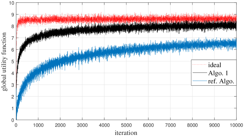
Figure 5: Evolution of the utility function, average results by 500 simulations

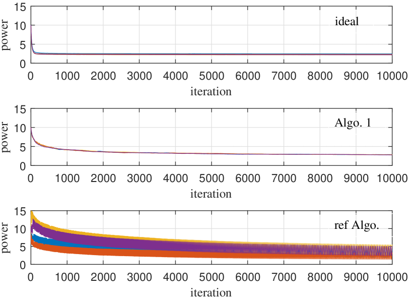
Figure 6: Evolution of power (action) of 4 nodes, average results by 500 simulations

Now we consider the situation where each node has incomplete collection of local utilities. We perform 100 independent simulation with $p\in\left\{1,0.5,0.25,0.1\right\}$. Recall that $p$ defined in (29) represents the level of incompleteness. The results are shown in Figure 7. We can see that the convergence speed decreases as the value of $p$ goes smaller. Such influence is not significant even if $p=0.5$, $i.e.$, a node has only $50\%$ chance to know the local utility of another user, which reduces a lot the information exchange in the network. As the value of $p$ is very small, i.e., $p=0.1$, same trend of convergence can be observed, although the algorithm converges slowly. On the figure, we show the results obtained after up to $10^{4}$ iterations only, which explains why for $p=0.1$ the algorithm has not converged yet to the optimal solution.

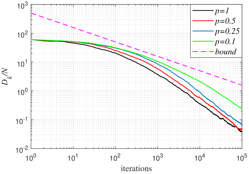
Figure 7: Evolution of $D_{k}/N$, average results by 100 simulations, with $p\in\left\{1,0.5,0.25,0.1\right\}$.

VIII-B Simulations with 10 nodes

In this section, we consider a more challenging case with $N=10$. We choose $\beta_{k}=2\left(k+1\right)^{-0.75}$ and $\gamma_{k}=12\left(k+1\right)^{-0.25}$. The results are presented in Figure 8 with $p\in\left\{1,0.5,0.25,0.1\right\}$, note that we have also plotted a line representing the optimum value of the average utility function. The shape of the curves in Figure 8 is similar to those in Figure 7. The algorithm converges slower as the number of nodes increases, yet the influence of the incompleteness of the received local utilities is less important.

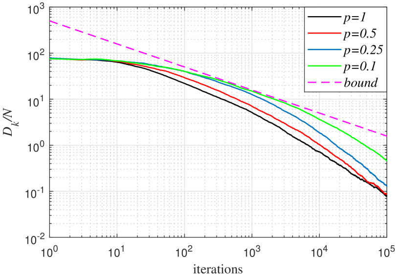
Figure 8: Evolution of $D_{k}/N$, average results by 100 simulations,with $p\in\left\{1,0.5,0.25,0.1\right\}$.

IX Conclusion

In this paper we have a challenging distributed optimization problems, under the assumption that only a numerical value of the stochastic state-dependent local utility function of the node is available at each time and nodes need to exchange their local values to optimize the total utilities of the network. We have developed fully distributed algorithms that converge to the optimum, in the situations where each node has the knowledge of all or only a part of the local utilities of the others. The convergence of our algorithms is examined by studying our algorithm using stochastic approximation technique. The convergence rate of the algorithms are derived. Numerical results are also provided for illustration.

-A Proof of Lemma 1

In this proof, we mainly need to find the relation between $\overline{\boldsymbol{g}}_{k}$ (the expected estimation of gradient) and $\nabla F\left(\boldsymbol{a}_{k}\right)$ (the actual gradient of the objective function), so that the upper bound of $\left\|\boldsymbol{b}_{k}\right\|$ can be derived.

From the definition of $\overline{\boldsymbol{g}}_{k}$, we have

$$\overline{\boldsymbol{g}}_{k} =\mathbb{E}_{\mathbf{S},\boldsymbol{\Phi},\boldsymbol{\eta}}\left(\boldsymbol{\Phi}_{k}\left(f\left(\boldsymbol{a}_{k}+\gamma_{k}\boldsymbol{\Phi}_{k},\mathbf{S}_{k}\right)+\sum_{i\in\mathcal{N}}\eta_{i,k}\right)\right)$$

$$=\mathbb{E}_{\boldsymbol{\Phi}}\left(\boldsymbol{\Phi}_{k}\mathbb{E}_{\mathbf{S}}\left(f\left(\boldsymbol{a}_{k}+\gamma_{k}\boldsymbol{\Phi}_{k},\mathbf{S}_{k}\right)\right)\right)$$

$$=\mathbb{E}_{\boldsymbol{\Phi}}\left(\boldsymbol{\Phi}_{k}F\left(\boldsymbol{a}_{k}+\gamma_{k}\boldsymbol{\Phi}_{k}\right)\right),$$ (52)

recall that the additive noise $\eta_{i,k}$ is zero mean and $F$ is the expected value of $f$ by definition.

Based on Taylor’s theorem and mean-valued theorem, there exists $\widetilde{\boldsymbol{a}}_{k}$ locating between $\boldsymbol{a}_{k}$ and $\boldsymbol{a}_{k}+c_{k}\boldsymbol{\Phi}_{k}$ such that

$$F\left(\boldsymbol{a}_{k}+\gamma_{k}\boldsymbol{\Phi}_{k}\right)=F\left(\boldsymbol{a}_{k}\right)+\!\sum_{j\in\mathcal{N}}\!\gamma_{k}\Phi_{j,t}F_{j}^{\prime}\left(\boldsymbol{a}_{k}\right)$$

$$\qquad\qquad\qquad+\sum_{j_{1},j_{2}\in\mathcal{N}}\frac{\gamma_{k}^{2}}{2}\Phi_{j_{1},k}\Phi_{j_{2},k}F_{j_{1},j_{2}}^{\prime\prime}\left(\widetilde{\boldsymbol{a}}_{k}\right).$$ (53)

Benefit from the properties of $\boldsymbol{\Phi}_{k}$ (A4), we have, $\forall i\in\mathcal{N}$,

$$\overline{g}_{i,k} =F\left(\boldsymbol{a}_{k}\right)\mathbb{E}_{\boldsymbol{\Phi}}\left(\Phi_{i,k}\right)+\gamma_{k}\sum_{j\in\mathcal{N}}F_{j}^{\prime}\left(\boldsymbol{a}_{k}\right)\mathbb{E}_{\boldsymbol{\Phi}}\left(\Phi_{i,k}\Phi_{j,k}\right)$$

$$\quad\qquad+\sum_{j_{1},j_{2}\in\mathcal{N}}\frac{\gamma_{k}^{2}}{2}\mathbb{E}_{\boldsymbol{\Phi}}\left(\Phi_{i,k}\Phi_{j_{1},k}\Phi_{j_{2},k}F_{j_{1},j_{2}}^{\prime\prime}\left(\widetilde{\boldsymbol{a}}_{k}\right)\right)$$

$$=\alpha_{2}\gamma_{k}\left(F_{i}^{\prime}\left(\boldsymbol{a}_{k}\right)+b_{i,k}\right),$$ (54)

from (52) and (53), with

$$b_{i,k}=\sum_{j_{1},j_{2}\in\mathcal{N}}\frac{\gamma_{k}}{2\alpha_{2}}\mathbb{E}_{\boldsymbol{\Phi}}\left(\Phi_{i,k}\Phi_{j_{1},k}\Phi_{j_{2},k}F_{j_{1},j_{2}}^{\prime\prime}\left(\widetilde{\boldsymbol{a}}_{k}\right)\right).$$

From assumptions A2 and A4, $\left|b_{i,k}\right|$ can be upper bounded by

$$\left|b_{i,k}\right| \leq\sum_{j_{1},j_{2}\in\mathcal{N}}\frac{\gamma_{k}}{2\alpha_{2}}\mathbb{E}_{\boldsymbol{\Phi}}\left(\left|\Phi_{i,k}\right|\cdot\left|\Phi_{j_{1},k}\right|\cdot\left|\Phi_{j_{2},k}\right|\cdot\left|F_{j_{1},j_{2}}^{\prime\prime}\left(\widetilde{\boldsymbol{a}}_{k}\right)\right|\right)$$

$$\leq\sum_{j_{1},j_{2}\in\mathcal{N}}\frac{\gamma_{k}}{2\alpha_{2}}\mathbb{E}_{\boldsymbol{\Phi}}\left(\alpha_{3}^{3}\alpha_{1}\right)$$

$$=\gamma_{k}N^{2}\frac{\alpha_{3}^{3}\alpha_{1}}{2\alpha_{2}},$$ (55)

then we can get (25). Thus $\left\|\boldsymbol{b}_{k}\right\|\rightarrow 0$ as $\gamma_{k}$ is vanishing, which concludes the proof.

-B Proof of Lemma 2

The proof of Lemma 2 is mainly by the application of Doob’s martingale inequality [31].

We first need to show that the sequence $\left\{\sum_{k=K}^{K^{\prime}}\beta_{k}\boldsymbol{e}_{k}\right\}_{K^{\prime}\geq K}$ is martingale, which is straightforward as $\widehat{\boldsymbol{g}}_{k}$ and $\widehat{\boldsymbol{g}}_{k^{\prime}}$ are independent if $k\neq k^{\prime}$ and

$$\mathbb{E}_{\mathbf{S},\boldsymbol{\Phi},\boldsymbol{\eta}}\left(\boldsymbol{e}_{k}\right)=\mathbb{E}_{\mathbf{S},\boldsymbol{\Phi},\boldsymbol{\eta}}\left(\widehat{\boldsymbol{g}}_{k}-\mathbb{E}_{\mathbf{S},\boldsymbol{\Phi},\boldsymbol{\eta}}\left(\widehat{\boldsymbol{g}}_{k}\right)\right)=\mathbf{0}.$$

Then, by Doob’s martingale inequality, for any positive constant $\rho$, we have

$$\mathbb{P}\left(\sup_{K^{\prime}\geq K}\left\|\sum_{k=K}^{K^{\prime}}\beta_{k}\boldsymbol{e}_{k}\right\|\geq\rho\right)$$

$$\leq\frac{1}{\rho^{2}}\mathbb{E}_{\mathbf{S},\boldsymbol{\Phi},\boldsymbol{\eta}}\left(\left\|\sum_{k=K}^{K^{\prime}}\beta_{k}\boldsymbol{e}_{k}\right\|^{2}\right)$$

$$=\frac{1}{\rho^{2}}\mathbb{E}_{\mathbf{S},\boldsymbol{\Phi},\boldsymbol{\eta}}\left(\sum_{k=K}^{K^{\prime}}\sum_{k^{\prime}=K}^{K^{\prime}}\beta_{k}\beta_{k^{\prime}}\boldsymbol{e}_{k}^{T}\cdot\boldsymbol{e}_{k^{\prime}}\right)$$

$$\overset{(a)}{=}\frac{1}{\rho^{2}}\mathbb{E}_{\mathbf{S},\boldsymbol{\Phi},\boldsymbol{\eta}}\left(\sum_{k=K}^{K^{\prime}}\left\|\beta_{k}\boldsymbol{e}_{k}\right\|^{2}\right)$$

$$\leq\frac{1}{\rho^{2}}\sum_{k=K}^{\infty}\mathbb{E}_{\mathbf{S},\boldsymbol{\Phi},\boldsymbol{\eta}}\left(\beta_{k}^{2}\left\|\widehat{\boldsymbol{g}}_{k}-\mathbb{E}_{\mathbf{S},\boldsymbol{\Phi},\boldsymbol{\eta}}\left(\widehat{\boldsymbol{g}}_{k}\right)\right\|^{2}\right)$$

$$=\frac{1}{\rho^{2}}\sum_{k=K}^{\infty}\beta_{k}^{2}\left(\mathbb{E}_{\mathbf{S},\boldsymbol{\Phi},\boldsymbol{\eta}}\left(\left\|\widehat{\boldsymbol{g}}_{k}\right\|^{2}\right)-\left\|\mathbb{E}_{\mathbf{S},\boldsymbol{\Phi},\boldsymbol{\eta}}\left(\widehat{\boldsymbol{g}}_{k}\right)\right\|^{2}\right)$$

$$\leq\frac{1}{\rho^{2}}\sum_{k=K}^{\infty}\beta_{k}^{2}\mathbb{E}_{\mathbf{S},\boldsymbol{\Phi},\boldsymbol{\eta}}\left(\left\|\widehat{\boldsymbol{g}}_{k}\right\|^{2}\right)$$

$$\overset{\left(b\right)}{\leq}\frac{M}{\rho^{2}}\sum_{k=K}^{\infty}\beta_{k}^{2}$$ (56)

where $(a)$ holds as $\mathbb{E}\left(\boldsymbol{e}_{k}^{T}\cdot\boldsymbol{e}_{k^{\prime}}\right)=0$ for any $k\neq k^{\prime}$ and $(b)$ is by Lemma 6 as stated and proved in the end of this section. Since $\lim_{K\rightarrow\infty}\sum_{k=K}^{\infty}\beta_{k}^{2}=0$ by Assumption A4 and $M$ is bounded, we have $\frac{M}{\rho^{2}}\sum_{k=K}^{\infty}\beta_{k}^{2}$ vanishing for any bounded constant $\rho$. Therefore, the probability that $\left\|\sum_{k=K}^{K^{\prime}}\beta_{k}\boldsymbol{e}_{k}\right\|\geq\rho$ is also vanishing, which concludes the proof.

Lemma 6.

If all the conditions in A1-A5 are satisfied and $\left\|\boldsymbol{a}_{k}\right\|<\infty$ almost surely, then there exists a bounded constant $M>0$, such that $\mathbb{E}_{\mathbf{S},\boldsymbol{\Phi},\boldsymbol{\eta}}\left(\left\|\widehat{\boldsymbol{g}}_{k}\right\|^{2}\right)<M$ almost surely.

Proof:

For any $i\in\mathcal{N}$, we evaluate

$$\mathbb{E}_{\mathbf{S},\boldsymbol{\Phi},\boldsymbol{\eta}}\left(\widehat{g}_{i,k}^{2}\right)$$

$$=\mathbb{E}_{\mathbf{S},\boldsymbol{\Phi},\boldsymbol{\eta}}\left(\left(\Phi_{i,k}f\left(\boldsymbol{a}_{k}+\gamma_{k}\boldsymbol{\Phi}_{k},\mathbf{S}_{k}\right)+\Phi_{i,k}\sum_{j\in\mathcal{N}}\eta_{j,k}\right)^{2}\right)$$

$$\overset{(a)}{=}\mathbb{E}_{\mathbf{S},\boldsymbol{\Phi}}\left(\left(\Phi_{i,k}f\left(\boldsymbol{a}_{k}+\gamma_{k}\boldsymbol{\Phi}_{k},\mathbf{S}_{k}\right)\right)^{2}\right)+N\alpha_{2}\alpha_{4}$$

$$\overset{(b)}{\leq}\alpha_{3}^{2}\mathbb{E}_{\mathbf{S},\boldsymbol{\Phi}}\left(\left(f\left(\boldsymbol{a}_{k}+\gamma_{k}\boldsymbol{\Phi}_{k},\mathbf{S}_{k}\right)\right)^{2}\right)+N\alpha_{2}\alpha_{4}$$

$$\overset{(c)}{\leq}\alpha_{3}^{2}\mathbb{E}_{\mathbf{S},\boldsymbol{\Phi}}\!\left(\!\left(\left\|f\left(\mathbf{0},\mathbf{S}_{k}\right)\right\|+\!NL_{\mathbf{S}_{k}}\!\left\|\boldsymbol{a}_{k}+\gamma_{k}\boldsymbol{\Phi}_{k}\right\|\right)^{2}\!\right)\!+N\alpha_{2}\alpha_{4}$$

$$\overset{(d)}{\leq}2\alpha_{3}^{2}\mathbb{E}_{\mathbf{S}}\left(\mu_{\mathbf{S}_{k}}^{2}+N^{2}L_{\mathbf{S}_{k}}^{2}\left(\left\|\boldsymbol{a}_{k}\right\|+\gamma_{k}N^{\frac{1}{2}}\alpha_{3}\right)^{2}\right)+N\alpha_{2}\alpha_{4}$$

$$\overset{(e)}{=}2\alpha_{3}^{2}\left(\mu+N^{2}L\left(\left\|\boldsymbol{a}_{k}\right\|+\gamma_{k}N^{\frac{1}{2}}\alpha_{3}\right)^{2}\right)+N\alpha_{2}\alpha_{4}$$

$$<\infty$$ (57)

where $(a)$ is due to $\mathbb{E}_{\boldsymbol{\Phi},\boldsymbol{\eta}}\left(\left(\Phi_{i,k}\sum_{j\in\mathcal{N}}\eta_{j,k}\right)^{2}\right)=N\alpha_{2}\alpha_{4}$ and $(b)$ is by Assumption A4. From (10), we have

$$\left\|f\left(\boldsymbol{a},\mathbf{S}\right)\right\|-\left\|f\left(\boldsymbol{0},\mathbf{S}\right)\right\|\leq\left\|f\left(\boldsymbol{a},\mathbf{S}\right)-f\left(\boldsymbol{0},\mathbf{S}\right)\right\|\leq NL_{\mathbf{S}}\left\|\boldsymbol{a}\right\|,$$

so $\left\|f\left(\boldsymbol{a},\mathbf{S}\right)\right\|\leq\left\|f\left(\boldsymbol{0},\mathbf{S}\right)\right\|+NL_{\mathbf{S}}\left\|\boldsymbol{a}\right\|$, $(c)$ can be obtained. We denote $\mu_{\mathbf{S}_{k}}=\left\|f\left(\mathbf{0},\mathbf{S}_{k}\right)\right\|$ in $(d)$ and the inequality is because of $(x+y)/2\leq\sqrt{\left(x^{2}+y^{2}\right)/2}$, $\forall x,y\in\mathbb{R}$. In $(e)$, we introduce $\mu=\mathbb{E}_{\mathbf{S}}\left(\mu_{\mathbf{S}_{k}}^{2}\right)$ and $L=\mathbb{E}_{\mathbf{S}}\left(L_{\mathbf{S}_{k}}^{2}\right)$.

Based on (57), we see that $\mathbb{E}\left(\left\|\widehat{\boldsymbol{g}}_{k}\right\|^{2}\right)=\sum_{i\in\mathcal{N}}\mathbb{E}\left(\widehat{g}_{i,k}^{2}\right)$ is also bounded, which concludes the proof. ∎

-C Proof of Theorem 1

In this proof, we start with the evolution of the divergence $d_{k}$ as defined in (20), then we show that $d_{k}$ should be vanishing almost surely by applying Lemma 1 and Lemma 2.

By definition, we have

$$d_{k+1} =\left\|\boldsymbol{a}_{k+1}-\boldsymbol{a}^{*}\right\|^{2}=\left\|\boldsymbol{a}_{k}+\beta_{k}\widehat{\boldsymbol{g}}_{k}-\boldsymbol{a}^{*}\right\|^{2}$$

$$=d_{k}+\beta_{k}^{2}\left\|\widehat{\boldsymbol{g}}_{k}\right\|^{2}+2\beta_{k}\left(\boldsymbol{a}_{k}-\boldsymbol{a}^{*}\right)^{T}\cdot\widehat{\boldsymbol{g}}_{k}.$$ (58)

We sum both sides of (58) to obtain

$$d_{K+1} =d_{0}+\sum_{k=0}^{K}\left(\beta_{k}^{2}\left\|\widehat{\boldsymbol{g}}_{k}\right\|^{2}+2\beta_{k}\left(\boldsymbol{a}_{k}-\boldsymbol{a}^{*}\right)^{T}\cdot\widehat{\boldsymbol{g}}_{k}\right).$$ (59)

Consider (21), we can rewrite (59) as

$$d_{K+1} =d_{0}+\sum_{k=0}^{K}\beta_{k}^{2}\left\|\widehat{\boldsymbol{g}}_{k}\right\|^{2}+2\sum_{k=0}^{K}\beta_{k}\left(\boldsymbol{a}_{k}-\boldsymbol{a}^{*}\right)^{T}\cdot\boldsymbol{e}_{k}$$

$$+2\alpha_{2}\sum_{k=0}^{K}\beta_{k}\gamma_{k}\left(\boldsymbol{a}_{k}-\boldsymbol{a}^{*}\right)^{T}\cdot\left(\nabla F\left(\boldsymbol{a}_{k}\right)+\boldsymbol{b}_{k}\right).$$ (60)

As stated in Lemma 2, we have $\lim_{K\rightarrow\infty}\left\|\sum_{k=0}^{K}\beta_{k}\boldsymbol{e}_{k}\right\|<\infty$ (a.s.), besides $\left\|\boldsymbol{a}_{k}-\boldsymbol{a}^{*}\right\|<\infty$ a.s., thus

$$\lim_{K\rightarrow\infty}\left\|\sum_{k=0}^{K}\beta_{k}\left(\boldsymbol{a}_{k}-\boldsymbol{a}^{*}\right)^{T}\cdot\boldsymbol{e}_{k}\right\|<\infty,\quad\textrm{a.s.}$$ (61)

From Lemma 6, we have $\left\|\widehat{\boldsymbol{g}}_{k}\right\|^{2}<\infty$ almost surely. Then, by A5, the following holds almost surely as well,

$$\lim_{K\rightarrow\infty}\sum_{k=0}^{K}\beta_{k}^{2}\left\|\widehat{\boldsymbol{g}}_{k}\right\|^{2}<\infty.$$ (62)

From the above equations (60)-(62), we conclude that there exists $W<\infty$ such that $d_{K+1}\leq W+z_{K}$, with

$$z_{K}=2\alpha_{2}\sum_{k=0}^{K}\beta_{k}\gamma_{k}\left(\boldsymbol{a}_{k}-\boldsymbol{a}^{*}\right)^{T}\cdot\left(\nabla F\left(\boldsymbol{a}_{k}\right)+\boldsymbol{b}_{k}\right).$$ (63)

Since $d_{K+1}\geq 0$ by definition, we have $z_{K}>-\infty$.

Recheck (55), we can say that for an arbitrary small positive value $\varepsilon_{b}$, there exists $K_{b}$ such that,

$$\left\|\nabla F\left(\boldsymbol{a}_{k}\right)+\boldsymbol{b}_{k}\right\|\geq\left(1-\varepsilon_{b}\right)\left\|\nabla F\left(\boldsymbol{a}_{k}\right)\right\|,\>\forall k\geq K_{b},$$ (64)

which also implies that $\left(\boldsymbol{a}_{k}-\boldsymbol{a}^{*}\right)^{T}\cdot\left(\nabla F\left(\boldsymbol{a}_{k}\right)+\boldsymbol{b}_{k}\right)\leq 0$, $\forall k\geq K_{b}$, by the concavity of $F$ in (7). Therefore $0\leq d_{K+1}<\infty$ for any large $K$ and $\lim_{K\rightarrow\infty}d_{K+1}=\overline{d}$ exists. The following steps of the proof is similar to the classical proof in [32].

Assume that: H1) $\overline{d}>0$, i.e., $\boldsymbol{a}_{k}$ does not converge to $\boldsymbol{a}^{*}$, then for any $\varepsilon_{h}>0$, there exists $K_{h}$ such that

$$\left(\boldsymbol{a}_{k}-\boldsymbol{a}^{*}\right)^{T}\cdot\nabla F\left(\boldsymbol{a}_{k}\right)<-\varepsilon_{h},\quad\forall k\geq K_{h}.$$ (65)

From (63) and (64), we get that $\forall k\geq K_{m}=\max\left\{K_{h},K_{b}\right\}$,

$$\left(\boldsymbol{a}_{k}-\boldsymbol{a}^{*}\right)^{T}\cdot\left(\nabla F\left(\boldsymbol{a}_{k}\right)+\boldsymbol{b}_{k}\right)<-\varepsilon_{h}\left(1-\varepsilon_{b}\right),$$ (66)

which leads to

$$\lim_{K\rightarrow\infty}\sum_{k=K_{m}}^{K}\beta_{k}\gamma_{k}\left(\boldsymbol{a}_{k}-\boldsymbol{a}^{*}\right)^{T}\cdot\left(\nabla F\left(\boldsymbol{a}_{k}\right)+\boldsymbol{b}_{k}\right)$$

$$<-\varepsilon_{h}\left(1-\varepsilon_{b}\right)\lim_{K\rightarrow\infty}\sum_{k=K_{m}}^{K}\beta_{k}\gamma_{k}<-\infty,$$ (67)

as $\sum\beta_{k}\gamma_{k}$ diverges by assumption A4.

We find that $z_{K}<-\infty$ and $d_{K+1}<-\infty$. However $d_{K+1}$ should be positive by definition. Therefore, the hypothesis H1 cannot be true, there should be $\lim_{k\rightarrow\infty}d_{k}=0$, $\lim_{k\rightarrow\infty}\nabla F\left(\boldsymbol{a}_{k}\right)=\mathbf{0}$, and $\lim_{k\rightarrow\infty}\boldsymbol{a}_{k}=\boldsymbol{a}^{*}$ almost surely, which concludes the proof.

-D Proof of Theorem 2

We learn first the property of the projection (28) in order to find an efficient way to simplify the proof. Otherwise, as stated in Remark 3, the proof can be complicated.

Define $\mathcal{C}_{i,k}=\left[a_{i,\min}+\alpha_{3}\gamma_{k},a_{i,\max}-\alpha_{3}\gamma_{k}\right]$ for any $i\in\mathcal{N}$ and $\mathcal{C}_{k}=\mathcal{C}_{1,k}\times\ldots\times\mathcal{C}_{N,k}$. Obviously, $\mathtt{Proj}\left(\boldsymbol{a}_{k}+\beta_{k}\widehat{\boldsymbol{g}}_{k}\right)\in\mathcal{C}_{k+1}$ by (28). Since $\gamma_{k}$ is a decreasing sequence, we find that $\mathcal{C}_{k}\subseteq\mathcal{C}_{k+1}$. Furthermore, we have $\lim_{k\rightarrow\infty}\mathcal{C}_{k}=\left[0,a_{\max}\right]^{N}$ as $\lim_{k\rightarrow\infty}\gamma_{k}=0$. Hence, there exists $K_{\mathrm{c}}\in\mathbb{N}$, such that $\boldsymbol{a}^{*}\in\mathcal{C}_{k+1}$ for any $k\geq K_{\mathrm{c}}$. It is straightforward to prove that

$$\left\|\mathtt{Proj}\left(\boldsymbol{a}_{k}+\beta_{k}\widehat{\boldsymbol{g}}_{k}\right)-\boldsymbol{a}^{*}\right\|\leq\left\|\boldsymbol{a}_{k}+\beta_{k}\widehat{\boldsymbol{g}}_{k}-\boldsymbol{a}^{*}\right\|,\>\forall k\geq K_{\mathrm{c}},$$

meaning that the projection makes $\boldsymbol{a}_{k+1}$ closer to $\boldsymbol{a}^{*}$ in the Euclidean space when $\boldsymbol{a}_{k+1}\in\mathcal{C}_{k+1}$ and $\boldsymbol{a}^{*}\in\mathcal{C}_{k+1}$.

Re-consider the divergence as defined in (20), we have

$$d_{k+1} =\left\|\mathtt{Proj}\left(\boldsymbol{a}_{k}+\beta_{k}\widehat{\boldsymbol{g}}_{k}\right)-\boldsymbol{a}^{*}\right\|^{2}.$$

$$\leq\left\|\boldsymbol{a}_{k}+\beta_{k}\widehat{\boldsymbol{g}}_{k}-\boldsymbol{a}^{*}\right\|^{2},\quad\forall k\geq K_{\mathrm{c}}.$$ (68)

from which we get

$$d_{K+1}\leq d_{K_{\mathrm{c}}}+\sum_{k=K_{\mathrm{c}}}^{K}\beta_{k}^{2}\left\|\widehat{\boldsymbol{g}}_{k}\right\|^{2}+2\sum_{k=K_{\mathrm{c}}}^{K}\beta_{k}\left(\boldsymbol{a}_{k}-\boldsymbol{a}^{*}\right)^{T}\cdot\boldsymbol{e}_{k}$$

$$\qquad+2\alpha_{2}\sum_{k=K_{\mathrm{c}}}^{K}\beta_{k}\gamma_{k}\left(\boldsymbol{a}_{k}-\boldsymbol{a}^{*}\right)^{T}\cdot\left(\nabla F\left(\boldsymbol{a}_{k}\right)+\boldsymbol{b}_{k}\right),$$ (69)

where $\boldsymbol{b}_{k}$ and $\boldsymbol{e}_{k}$ are the same as those defined in (23) and (24). The results presented in Lemma 1 and in Lemma 2 are valid as well.

Clearly, (69) has similar shape compared with (60). Using similar steps in Appendix -C, Theorem 2 can be proved.

-E Proof of Lemma 3

We start with the conditional expectation, based on (30), we have

$$\mathbb{E}_{\mathcal{I}_{i,k}}\left(\widetilde{f}_{i}^{(\textrm{I})}\left(\boldsymbol{a},\mathbf{S}_{k},\mathcal{I}_{i,k}\right)\big{|}\left|\mathcal{I}_{i,k}\right|=n\right)$$

$$=\begin{cases}\widetilde{u}_{i,k}+\frac{N-1}{n}\mathbb{E}_{\mathcal{I}_{i,k}}\left(\sum_{j\in\mathcal{I}_{i,k}}\widetilde{u}_{j,k}\big{|}\left|\mathcal{I}_{i,k}\right|=n\right),&\textrm{if }n\neq 0,\\ 0,&\textrm{if }n=0.\end{cases}$$ (70)

Denote $\mathcal{U}_{i}^{\left(n\right)}$ as a collection of all possible sets $\mathcal{I}_{i,k}$ such that $\left|\mathcal{I}_{i,k}\right|=n$, e.g., $\mathcal{U}_{i}^{\left(1\right)}=\left\{\left\{1\right\},\ldots,\left\{i-1\right\},\left\{i+1\right\},\ldots\right\}$. Since each node has an equal probability to be involved in $\mathcal{I}_{i,k}$, the sets in $\mathcal{U}_{i}^{\left(n\right)}$ are also equiprobable, i.e.,

$$\mathbb{P}\left(\mathcal{I}_{i,k}=\mathcal{I}\big{|}\left|\mathcal{I}_{i,k}\right|=n\right)=\frac{1}{\binom{N-1}{n}},\quad\forall\mathcal{I}\in\mathcal{U}_{i}^{\left(n\right)},$$

note that the cardinal of $\mathcal{U}_{i}^{\left(n\right)}$ is $\binom{N-1}{n}$. We evaluate

$$\mathbb{E}_{\mathcal{I}_{i,k}}\left(\sum_{j\in\mathcal{I}_{i,k}}\widetilde{u}_{j,k}\bigg{|}\left|\mathcal{I}_{i,k}\right|=n\right)$$

$$=\sum_{\mathcal{I}\in\mathcal{U}_{i}^{\left(n\right)}}\frac{1}{\binom{N-1}{n}}\sum_{j\in\mathcal{I}}\widetilde{u}_{j,k}=\frac{1}{\binom{N-1}{n}}\frac{n\binom{N-1}{n}}{N-1}\sum_{j\in\mathcal{N}\setminus\left\{i\right\}}\widetilde{u}_{j,k}$$

$$=\frac{n}{N-1}\sum_{j\in\mathcal{N}\setminus\left\{i\right\}}\widetilde{u}_{j,k}.$$ (71)

Combine (70) and (71), for any $n\in\left\{1,\ldots,N-1\right\}$, we have

$$\mathbb{E}_{\mathcal{I}_{i,k}}\left(\widetilde{f}_{i}^{(\textrm{I})}\left(\boldsymbol{a},\mathbf{S}_{k},\mathcal{I}_{i,k}\right)\big{|}\left|\mathcal{I}_{i,k}\right|=n\right) =\widetilde{f}\left(\boldsymbol{a},\mathbf{S}_{k}\right).$$ (72)

According to the basic rule of expectation,

$$\mathbb{E}\left(\widetilde{f}_{i}^{(\textrm{I})}\left(\boldsymbol{a},\mathbf{S}_{k},\mathcal{I}_{i,k}\right)\right)$$

$$=\sum_{n=0}^{N-1}\mathbb{P}\left(\left|\mathcal{I}_{i,k}\right|=n\right)\mathbb{E}_{\mathcal{I}_{i,k}}\left(\widetilde{f}_{i}^{(\textrm{I})}\left(\boldsymbol{a},\mathbf{S}_{k},\mathcal{I}_{i,k}\right)\big{|}\left|\mathcal{I}_{i,k}\right|=n\right)$$

$$=\sum_{n=1}^{N-1}\mathbb{P}\left(\left|\mathcal{I}_{i,k}\right|=n\right)\widetilde{f}\left(\boldsymbol{a},\mathbf{S}_{k}\right)$$

$$=\left(1-\mathbb{P}\left(\left|\mathcal{I}_{i,k}\right|=0\right)\right)\widetilde{f}\left(\boldsymbol{a},\mathbf{S}_{k}\right)$$

$$=\left(1-(1-p)^{N}\right)\widetilde{f}\left(\boldsymbol{a},\mathbf{S}_{k}\right),$$

which concludes the proof.

-F Proof of Theorem 3

As the analysis in Section V-C, we mainly need to check:

• C1) whether $b_{i,k}^{\left(\textrm{I}\right)}$ is vanishing;

• C2) whether $\sum_{k=1}^{\infty}\beta_{k}\boldsymbol{e}_{k}^{\left(\textrm{I}\right)}$ converges.

The proof of these two statements are more complicated as compared to Appendix -A and Appendix -B, since there is an additional random term $\mathcal{I}_{i,k}$ in both $b_{i,k}^{\left(\textrm{I}\right)}$ and $e_{i,k}^{\left(\textrm{I}\right)}$, compared with $b_{i,k}$ and $e_{i,k}$ discussed in Section V. Then Theorem 3 can be proved in the end.

-F1 Proof of C1

We start with the bias term, by Lemma 3, we have

$$\mathbb{E}_{\mathbf{S},\boldsymbol{\Phi},\boldsymbol{\eta},\mathcal{I}_{i,k}}\left(\widehat{g}_{i,k}^{(\textrm{I})}\right) =\mathbb{E}_{\mathbf{S},\boldsymbol{\Phi},\boldsymbol{\eta},\mathcal{I}_{i,k}}\left(\Phi_{i,k}\widetilde{f}_{i}^{(\textrm{I})}\left(\boldsymbol{a},\mathbf{S}_{k},\mathcal{I}_{i,k}\right)\right)$$

$$=q\mathbb{E}_{\mathbf{S},\boldsymbol{\Phi},\boldsymbol{\eta}}\left(\Phi_{i,k}\widetilde{f}\left(\boldsymbol{a},\mathbf{S}_{k}\right)\right).$$

We then find that $b_{i,k}^{\left(\textrm{I}\right)}$ in this section is the same as $b_{i,k}$ defined in (23), as

$$b_{i,k}^{\left(\textrm{I}\right)} =\frac{q\mathbb{E}_{\mathbf{S},\boldsymbol{\Phi},\boldsymbol{\eta}}\left(\Phi_{i,k}\widetilde{f}\left(\boldsymbol{a},\mathbf{S}_{k}\right)\right)}{q\alpha_{2}\gamma_{k}}-F_{i}^{\prime}\left(\boldsymbol{a}_{k}\right)$$

$$=b_{i,k}.$$ (73)

Therefore, $b_{i,k}^{\left(\textrm{I}\right)}$ can be vanishing as $\gamma_{k}$ is vanishing according to Lemma 1, C1 is verified.

-F2 Proof of C2

The second step is to analyze the stochastic noise to check C2. From the definition (36) , we have

$$\mathbb{E}_{\mathbf{S},\boldsymbol{\Phi},\boldsymbol{\eta},\mathcal{I}_{i,k}}\left(e_{i,k}^{\left(\textrm{I}\right)}\right) =\mathbb{E}_{\mathbf{S},\boldsymbol{\Phi},\boldsymbol{\eta},\mathcal{I}_{i,k}}\left(\widehat{g}_{i,k}^{\left(\textrm{I}\right)}-\mathbb{E}_{\mathbf{S},\boldsymbol{\Phi},\boldsymbol{\eta},\mathcal{I}_{i,k}}\left(\widehat{g}_{i,k}^{\left(\textrm{I}\right)}\right)\right)$$

$$=0.$$

As $\mathcal{I}_{i,k}$ and $\mathcal{I}_{i,k^{\prime}}$ are independent for any $k\neq k^{\prime}$, the sequence $\left\{\sum_{k=K}^{K^{\prime}}\gamma_{k}\boldsymbol{e}_{k}^{\left(\textrm{I}\right)}\right\}_{K^{\prime}\geq K}$ is martingale. By applying Doob’s inequality, we have

$$\mathbb{P}\left(\sup_{K^{\prime}\geq K}\left\|\sum_{k=K}^{K^{\prime}}\beta_{k}\boldsymbol{e}_{k}^{\left(\textrm{I}\right)}\right\|\geq\rho\right)$$

$$\leq\frac{1}{\rho^{2}}\mathbb{E}_{\mathbf{S},\boldsymbol{\Phi},\boldsymbol{\eta},\mathcal{I}_{i,k}}\left(\left\|\sum_{k=K}^{K^{\prime}}\beta_{k}\boldsymbol{e}_{k}\right\|^{2}\right)$$

$$\overset{\left(a\right)}{\leq}\frac{1}{\rho^{2}}\sum_{k=K}^{\infty}\beta_{k}^{2}\sum_{i\in\mathcal{N}}\mathbb{E}_{\mathbf{S},\boldsymbol{\Phi},\boldsymbol{\eta},\mathcal{I}_{i,k}}\left(\left(\widehat{g}_{i,k}^{\left(\textrm{I}\right)}\right)^{2}\right),$$ (74)

where $\left(a\right)$ can be obtained using similar steps in (56). In order to evaluate the average of $\left(\widehat{g}_{i,k}^{\left(\textrm{I}\right)}\right)^{2}$, we need to consider, for any $n\in\left\{1,\ldots,N-1\right\}$,

$$\mathbb{E}_{\mathcal{I}_{i,k}}\left(\left(\widehat{g}_{i,k}^{\left(\textrm{I}\right)}\right)^{2}\big{|}\left|\mathcal{I}_{i,k}\right|=n\right)$$

$$=\Phi_{i,k}^{2}\mathbb{E}_{\mathcal{I}_{i,k}}\left(\left.\left(\widetilde{u}_{i,k}+\frac{N-1}{n}\sum_{j\in\mathcal{I}_{i,k}}\widetilde{u}_{j,k}\right)^{2}\right|\left|\mathcal{I}_{i,k}\right|=n\right)$$

$$\overset{(a)}{\leq}\alpha_{3}^{2}\left(n+1\right)\left(\widetilde{u}_{i,k}^{2}+\left(\frac{N-1}{n}\right)^{2}\cdot\right.$$

$$\qquad\qquad\qquad\qquad\left.\mathbb{E}_{\mathcal{I}_{i,k}}\left(\left.\sum_{j\in\mathcal{I}_{i,k}}\widetilde{u}_{j,k}^{2}\right|\left|\mathcal{I}_{i,k}\right|=n\right)\right)$$

$$\overset{(b)}{=}\alpha_{3}^{2}\left(n+1\right)\left(\widetilde{u}_{i,k}^{2}+\frac{N-1}{n}\sum_{j\in\mathcal{N}\setminus\left\{i\right\}}\widetilde{u}_{j,k}^{2}\right)$$

$$\overset{(c)}{\leq}\alpha_{3}^{2}\left(\left(n+1\right)\widetilde{u}_{i,k}^{2}+2\left(N-1\right)\sum_{j\in\mathcal{N}\setminus\left\{i\right\}}\widetilde{u}_{j,k}^{2}\right),$$ (75)

where $(a)$ is by $\Phi_{i,k}^{2}\leq\alpha_{3}^{2}$ and $\sum_{i=1}^{m}x_{i}/m\leq\sqrt{\sum_{i=1}^{m}x_{i}^{2}/m}$, $(b)$ can be proved using the same way as (71), and $(c)$ is due to $1<\left(n+1\right)/n\leq 2$ as $1\leq n\leq N-1$.

Since $\widehat{g}_{i,k}^{\left(\textrm{I}\right)}=0$ as $n=0$ by definition, we have

$$\mathbb{E}_{\mathcal{I}_{i,k}}\left(\left(\widehat{g}_{i,k}^{\left(\textrm{I}\right)}\right)^{2}\right)$$

$$=\sum_{n=1}^{N-1}\mathbb{P}\left(\left|\mathcal{I}_{i,k}\right|=n\right)\mathbb{E}_{\mathcal{I}_{i,k}}\left(\left.\left(\widehat{g}_{i,k}^{\left(\textrm{I}\right)}\right)^{2}\right|\left|\mathcal{I}_{i,k}\right|=n\right)$$

$$\leq\mathbb{E}_{\mathcal{I}_{i,k}}\left(\left|\mathcal{I}_{i,k}\right|\right)\alpha_{3}^{2}\widetilde{u}_{i,k}^{2}+$$

$$\qquad\mathbb{P}\left(\left|\mathcal{I}_{i,k}\right|\neq 0\right)\cdot\alpha_{3}^{2}\left(\widetilde{u}_{i,k}^{2}+2\left(N-1\right)\sum_{j\in\mathcal{N}\setminus\left\{i\right\}}\widetilde{u}_{j,k}^{2}\right)$$

$$=\alpha_{3}^{2}\left(\left(p\left(N-1\right)+q\right)\widetilde{u}_{i,k}^{2}+2\left(N-1\right)q\sum_{j\in\mathcal{N}\setminus\left\{i\right\}}\widetilde{u}_{j,k}^{2}\right),$$ (76)

where $\mathbb{E}_{\mathcal{I}_{i,k}}\left(\left|\mathcal{I}_{i,k}\right|\right)=\left(N-1\right)p$ and $q=\mathbb{P}\left(\left|\mathcal{I}_{i,k}\right|\neq 0\right)$ is defined in (33).

We also need to find a upper bound of $\mathbb{E}_{\mathbf{S},\boldsymbol{\Phi},\boldsymbol{\eta}}\left(\widetilde{u}_{i,k}^{2}\right)$ for any $i\in\mathcal{N}$, the following steps are similar to (57),

$$\mathbb{E}_{\mathbf{S},\boldsymbol{\Phi},\boldsymbol{\eta}}\left(\widetilde{u}_{i,k}^{2}\right)$$

$$=\mathbb{E}_{\mathbf{S},\boldsymbol{\Phi},\boldsymbol{\eta}}\left(\left(u_{i}\left(\boldsymbol{a}_{k}+\gamma_{k}\boldsymbol{\Phi}_{k},\mathbf{S}_{k}\right)+\eta_{i,k}\right)^{2}\right)$$

$$=\mathbb{E}_{\mathbf{S},\boldsymbol{\Phi}}\left(\left(u_{i}\left(\boldsymbol{a}_{k}+\gamma_{k}\boldsymbol{\Phi}_{k},\mathbf{S}_{k}\right)\right)^{2}\right)+\alpha_{4}$$

$$\overset{(a)}{\leq}\mathbb{E}_{\mathbf{S},\boldsymbol{\Phi}}\left(\left(\left\|u_{i}\left(\mathbf{0},\mathbf{S}_{k}\right)\right\|+L_{\mathbf{S}_{k}}\left\|\boldsymbol{a}_{k}+\gamma_{k}\boldsymbol{\Phi}_{k}\right\|\right)^{2}\right)+\alpha_{4}$$

$$\overset{(b)}{\leq}2\mathbb{E}_{\mathbf{S}}\left(\iota_{\mathbf{S}_{k}}^{2}+L_{\mathbf{S}_{k}}^{2}\left(\left\|\boldsymbol{a}_{k}\right\|+\sqrt{N}\gamma_{k}\alpha_{3}\right)^{2}\right)+\alpha_{4}$$

$$\overset{(c)}{=}2\left(\iota+L\left(\left\|\boldsymbol{a}_{k}\right\|+\sqrt{N}\gamma_{k}\alpha_{3}\right)^{2}\right)+\alpha_{4}<\infty$$ (77)

where: $(a)$ is by (10); in $(b)$, we introduce $\iota_{\mathbf{S}_{k}}=\max_{i\in\mathcal{N}}\left\{\left\|u_{i}\left(\mathbf{0},\mathbf{S}_{k}\right)\right\|\right\}<\infty$ as an bounded upper bound of $\left\|u_{i}\left(\mathbf{0},\mathbf{S}_{k}\right)\right\|$; in $(c)$, we denote $\iota=\mathbb{E}_{\mathbf{S}}\left(\iota_{\mathbf{S}_{k}}^{2}\right)$ and $L=\mathbb{E}_{\mathbf{S}}\left(L_{\mathbf{S}_{k}}^{2}\right)$. Note that the upper bound (77) is valid for any $i\in\mathcal{N}$.

Based on (76) and (77), we evaluate

$$\mathbb{E}_{\mathbf{S},\boldsymbol{\Phi},\boldsymbol{\eta},\mathcal{I}_{i,k}}\left(\left(\widehat{g}_{i,k}^{\left(\textrm{I}\right)}\right)^{2}\right)$$

$$=\mathbb{E}_{\mathbf{S},\boldsymbol{\Phi},\boldsymbol{\eta}}\left(\mathbb{E}_{\mathcal{I}_{i,k}}\left(\left(\widehat{g}_{i,k}^{\left(\textrm{I}\right)}\right)^{2}\right)\right)$$

$$\leq\alpha_{3}^{2}\left(2\left(N-1\right)^{2}q+\left(N-1\right)p+q\right)\cdot$$

$$\qquad\qquad\left(2\left(\iota+L\left(\left\|\boldsymbol{a}_{k}\right\|+\sqrt{N}\gamma_{k}\alpha_{3}\right)^{2}\right)+\alpha_{4}\right)$$

$$<\infty.$$ (78)

From (74) and (78), we can conclude that $\sum_{k=1}^{\infty}\beta_{k}\boldsymbol{e}_{k}^{\left(\textrm{I}\right)}$ converges almost surely.

-F3 Proof of convergence

Finally, we can show the convergence of Algorithm 2. Consider the evolution of the divergence $d_{k}^{\left(\mathrm{I}\right)}=\left\|\boldsymbol{a}_{k}^{\left(\mathrm{I}\right)}-\boldsymbol{a}^{*}\right\|^{2}$, we get

$$d_{K+1}^{\left(\mathrm{I}\right)} =d_{0}+\sum_{k=0}^{K}\beta_{k}^{2}\left\|\widehat{\boldsymbol{g}}_{k}^{\left(\mathrm{I}\right)}\right\|^{2}+2\sum_{k=0}^{K}\beta_{k}\left(\boldsymbol{a}_{k}^{\left(\mathrm{I}\right)}-\boldsymbol{a}^{*}\right)^{T}\cdot\boldsymbol{e}_{k}^{\left(\mathrm{I}\right)}$$

$$+2\alpha_{2}\sum_{k=0}^{K}\beta_{k}\gamma_{k}\left(\boldsymbol{a}_{k}^{\left(\mathrm{I}\right)}-\boldsymbol{a}^{*}\right)^{T}\cdot\left(\nabla F\left(\boldsymbol{a}_{k}^{\left(\mathrm{I}\right)}\right)+\boldsymbol{b}_{k}^{\left(\mathrm{I}\right)}\right),$$ (79)

with the same shape as (60) and be obtained using the same steps. The following proof is also similar to that in Appendix -C, as we have already shown that $\boldsymbol{b}_{k}^{\left(\mathrm{I}\right)}$ and $\boldsymbol{e}_{k}^{\left(\mathrm{I}\right)}$ have similar properties as $\boldsymbol{b}_{k}$ and $\boldsymbol{e}_{k}$.

-G Proof of Lemma 4

We investigate the relation between the two successive average divergence. We mainly demonstrate (38), as the proof of (39) is quite similar.

In Algorithm 1, we have

$$D_{k+1}^{\left(\mathrm{C}\right)} =\mathbb{E}\left(\left\|\boldsymbol{a}_{k+1}-\boldsymbol{a}^{*}\right\|_{2}^{2}\right)=\mathbb{E}\left(\left\|\boldsymbol{a}_{k}+\beta_{k}\widehat{\boldsymbol{g}}_{k}-\boldsymbol{a}^{*}\right\|_{2}^{2}\right)$$

$$=D_{k}^{\left(\mathrm{C}\right)}+\beta_{k}^{2}\mathbb{E}\left(\left\|\widehat{\boldsymbol{g}}_{k}\right\|_{2}^{2}\right)+2\beta_{k}\mathbb{E}\left(\left(\boldsymbol{a}_{k}-\boldsymbol{a}^{*}\right)^{T}\widehat{\boldsymbol{g}}_{k}\right).$$ (80)

According to (57), we have shown that $\mathbb{E}\left(\left\|\widehat{\boldsymbol{g}}_{k}\right\|_{2}^{2}\right)<M^{\left(\mathrm{C}\right)}$ almost surely, with $M^{\left(\mathrm{C}\right)}$ a bounded constant. Meanwhile, we evaluate

$$\mathbb{E}\left(\left(\boldsymbol{a}_{k}-\boldsymbol{a}^{*}\right)^{T}\widehat{\boldsymbol{g}}_{k}\right) =\alpha_{2}\gamma_{k}\mathbb{E}\left(\left(\boldsymbol{a}_{k}-\boldsymbol{a}^{*}\right)^{T}\left(\nabla F\left(\boldsymbol{a}_{k}\right)+\boldsymbol{b}_{k}\right)\right),$$ (81)

which can be obtained by using (21) and $\mathbb{E}\left(\boldsymbol{e}_{k}\right)=\mathbf{0}$. We have

$$\left(\boldsymbol{a}_{k}-\boldsymbol{a}^{*}\right)^{T}\boldsymbol{b}_{k} \leq\sum_{i=1}^{N}\left|a_{i,k}-a_{i}^{*}\right|\left|b_{i,k}\right|$$

$$\leq N^{2}\frac{\alpha_{3}^{3}\alpha_{1}}{2\alpha_{2}}\gamma_{k}\sum_{i=1}^{N}\left|a_{i,k}-a_{i}^{*}\right|$$

$$\leq N^{2}\frac{\alpha_{3}^{3}\alpha_{1}}{2\alpha_{2}}\gamma_{k}\sqrt{N\sum_{i=1}^{N}\left(a_{i,k}-a_{i}^{*}\right)^{2}}$$

$$=N^{\frac{5}{2}}\frac{\alpha_{3}^{3}\alpha_{1}}{2\alpha_{2}}\gamma_{k}\left\|\boldsymbol{a}_{k}-\boldsymbol{a}^{*}\right\|_{2}.$$ (82)

From (81), (82), and the strong concavity (37), we have

$$\mathbb{E}\left(\left(\boldsymbol{a}_{k}-\boldsymbol{a}^{*}\right)^{T}\widehat{\boldsymbol{g}}_{k}\right)$$

$$\leq\alpha_{2}\gamma_{k}\mathbb{E}\left(-\alpha_{5}\left\|\boldsymbol{a}_{k}-\boldsymbol{a}^{*}\right\|_{2}^{2}+N^{\frac{5}{2}}\frac{\alpha_{3}^{3}\alpha_{1}}{2\alpha_{2}}\gamma_{k}\left\|\boldsymbol{a}_{k}-\boldsymbol{a}^{*}\right\|_{2}\right)$$

$$=-\alpha_{2}\alpha_{5}\gamma_{k}\mathbb{E}\left(\left\|\boldsymbol{a}_{k}-\boldsymbol{a}^{*}\right\|_{2}^{2}\right)$$

$$\qquad\qquad\qquad\qquad+N^{\frac{5}{2}}\frac{\alpha_{3}^{3}\alpha_{1}}{2}\gamma_{k}^{2}\sqrt{\left|\mathbb{E}\left(\left\|\boldsymbol{a}_{k}-\boldsymbol{a}^{*}\right\|_{2}\right)\right|^{2}}$$

$$=-\alpha_{2}\alpha_{5}\gamma_{k}D_{k}+\frac{1}{2}N^{\frac{5}{2}}\alpha_{3}^{3}\alpha_{1}\gamma_{k}^{2}\sqrt{D_{k}}.$$ (83)

By combining (80), (83) and the fact that $\mathbb{E}\left(\left\|\widehat{\boldsymbol{g}}_{k}\right\|_{2}^{2}\right)\leq M^{\left(\mathrm{C}\right)}$, we can obtain (38).

We have the similar steps to prove (39) for Algorithm 2, the main difference comes from the upper bound of $\mathbb{E}(\left\|\widehat{\boldsymbol{g}}_{k}^{\left(\mathrm{I}\right)}\right\|_{2}^{2})$ and

$$\mathbb{E}\left(\left(\boldsymbol{a}_{k}-\boldsymbol{a}^{*}\right)^{T}\widehat{\boldsymbol{g}}_{k}^{\left(\mathrm{I}\right)}\right)$$

$$=q\alpha_{2}\gamma_{k}\mathbb{E}\left(\left(\boldsymbol{a}_{k}-\boldsymbol{a}^{*}\right)^{T}\left(\nabla F\left(\boldsymbol{a}_{k}\right)+\boldsymbol{b}_{k}^{\left(\mathrm{I}\right)}\right)\right)$$

$$\leq q\left(-\alpha_{2}\alpha_{5}\gamma_{k}D_{k}+\frac{1}{2}N^{\frac{5}{2}}\alpha_{3}^{3}\alpha_{1}\gamma_{k}^{2}\sqrt{D_{k}}\right),$$ (84)

which is similar to (83) and the difference comes from the presence of the parameter $q$ in the generalized Robbins-Monro form (34), note that $\boldsymbol{b}_{k}^{\left(\mathrm{I}\right)}=\boldsymbol{b}_{k}$ as shown in (73).

-H Proof of Lemma 5

From (40) and $D_{k}\leq U_{k}$, we get

$$D_{k+1} \leq\left(1-A\beta_{k}\gamma_{k}\right)U_{k}+B\beta_{k}\gamma_{k}^{2}\sqrt{U_{k}}+C\beta_{k}^{2},$$

because $1-A\beta_{k}\gamma_{k}>0$ when $k\geq K_{0}$. In order to perform the induction, we need to have

$$\left(1-A\beta_{k}\gamma_{k}\right)U_{k}+B\beta_{k}\gamma_{k}^{2}\sqrt{U_{k}}+C\beta_{k}^{2}\leq U_{k+1}\leq U_{k},$$

which leads to

$$A\gamma_{k}U_{k}-B\gamma_{k}^{2}\sqrt{U_{k}}-C\beta_{k}\geq 0.$$ (85)

By solving (85), we obtain (43) as $\sqrt{U_{k}}>0$.

-I Proof of Theorem 4

We start with the proof of (46), which is realized by induction.

It is straightforward to get $D_{K_{0}}\leq\vartheta^{2}\gamma_{K_{0}}^{2}$ according to the definition of $\vartheta$. We mainly needs to verify that $D_{k}\leq\vartheta^{2}\gamma_{k}^{2}$ leads to $D_{k+1}\leq\vartheta^{2}\gamma_{k+1}^{2}$ for any $k\geq K_{0}$.

Suppose that $D_{k}\leq\vartheta^{2}\gamma_{k}^{2}$, from (40), we have

$$D_{k+1} \leq\left(1-A\beta_{k}\gamma_{k}\right)\gamma_{k}^{2}\vartheta^{2}+B\beta_{k}\gamma_{k}^{3}\vartheta+C\beta_{k}^{2}.$$

We then need to show that there exists $\vartheta\in\mathbb{R}^{+}$, such that

$$\left(1-A\beta_{k}\gamma_{k}\right)\gamma_{k}^{2}\vartheta^{2}+B\beta_{k}\gamma_{k}^{3}\vartheta+C\beta_{k}^{2} \leq U_{k+1}$$

$$=\vartheta^{2}\gamma_{k+1}^{2},$$

which can be written as

$$\left(\chi_{k}-A\right)\vartheta^{2}+B\vartheta+C\beta_{k}\gamma_{k}^{-3}\leq 0,$$ (86)

with $\chi_{k}=\frac{1-\left(\frac{\gamma_{k+1}}{\gamma_{k}}\right)^{2}}{\beta_{k}\gamma_{k}}>0$ as defined in (44). By assumptions presented in Theorem 4, $\chi_{k}-A<0$, we can deduce from the inequality (86) that $\vartheta\geq\overline{\vartheta}_{k}$, with

$$\vartheta\geq\overline{\vartheta}_{k}=\frac{B}{2\left(A-\chi_{k}\right)}+\sqrt{\left(\frac{B}{2\left(A-\chi_{k}\right)}\right)^{2}+C\frac{\beta_{k}\gamma_{k}^{-3}}{A-\chi_{k}}}.$$

recall that both $B$ and $C\beta_{k}\gamma_{k}^{-3}$ are positive by definition. Consider $\epsilon_{1}$ and $\epsilon_{2}$ as defined in (45), we have

$$2\overline{\vartheta}_{k} \leq\frac{B}{A-\epsilon_{1}}+\sqrt{\left(\frac{B}{A-\epsilon_{1}}\right)^{2}+\frac{4C\epsilon_{2}}{A-\epsilon_{1}}},$$

We can thus prove that $D_{k+1}\leq\vartheta^{2}\gamma_{k+1}^{2}$ with $\vartheta$ defined in (47).

Then we turn to prove (48). Similar to the previous situation, we have $D_{K_{0}}\leq\varrho^{2}\frac{\beta_{K_{0}}}{\gamma_{K_{0}}}$. For any $k\geq K_{0}$, if $D_{k}\leq\varrho^{2}\frac{\beta_{k}}{\gamma_{k}}$, then

$$D_{k+1} \leq\left(1-A\beta_{k}\gamma_{k}\right)\frac{\beta_{k}}{\gamma_{k}}\varrho^{2}+B\left(\beta_{k}\gamma_{k}\right)^{\frac{3}{2}}\varrho+C\beta_{k}^{2}.$$

A sufficient condition to ensure $D_{k+1}\leq\varrho^{2}\frac{\beta_{k+1}}{\gamma_{k+1}}$ is that

$$\left(1-A\beta_{k}\gamma_{k}\right)\frac{\beta_{k}}{\gamma_{k}}\varrho^{2}+B\left(\beta_{k}\gamma_{k}\right)^{\frac{3}{2}}\varrho+C\beta_{k}^{2}\leq\frac{\beta_{k+1}}{\gamma_{k+1}}\varrho^{2}.$$

Thus $\varrho$ should satisfy

$$\left(\frac{\frac{\beta_{k}}{\gamma_{k}}-\frac{\beta_{k+1}}{\gamma_{k+1}}}{\beta_{k}^{2}}-A\right)\varrho^{2}+B\beta_{k}^{-\frac{1}{2}}\gamma_{k}^{\frac{3}{2}}\varrho+C\leq 0$$

If $\frac{\beta_{k}}{\gamma_{k}}-\frac{\beta_{k+1}}{\gamma_{k+1}}<A\beta_{k}^{2},$ then the condition on $\varrho$ should be $\varrho\geq\overline{\varrho}_{k}$ with

$$\overline{\varrho}_{k}=\frac{B\beta_{k}^{-\frac{1}{2}}\gamma_{k}^{\frac{3}{2}}+\sqrt{\left(B\beta_{k}^{-\frac{1}{2}}\gamma_{k}^{\frac{3}{2}}\right)^{2}+4C\left(A-\varpi_{k}\right)}}{2\left(A-\varpi_{k}\right)},$$

where $\varpi_{k}=\beta_{k}^{-2}\left(\frac{\beta_{k}}{\gamma_{k}}-\frac{\beta_{k+1}}{\gamma_{k+1}}\right)>0$ as defined in (45). Consider $\epsilon_{3}$ and $\epsilon_{4}$ given in (45), we have

$$\overline{\varrho}_{k} \leq\frac{B\epsilon_{4}+\sqrt{\left(B\epsilon_{4}\right)^{2}+4C\left(A-\epsilon_{3}\right)}}{2\left(A-\epsilon_{3}\right)},$$

then we can prove (49).

-J Proof of Theorem 5

From Theorem 4, we can see that the order of the convergence rate mainly relies on $\nu_{1}$ and $\nu_{2}$, as $\gamma_{k}^{2}\propto\left(k+1\right)^{-2\nu_{2}}$ and $\frac{\beta_{k}}{\gamma_{k}}\propto\left(k+1\right)^{-\left(\nu_{1}-\nu_{2}\right)}$. However, before the conclusion, we should still verify two points:

• i) whether the conditions $\epsilon_{1}<A$ and $\epsilon_{3}<A$ are satisfied;

• ii) whether the constant terms $\vartheta$ and $\varrho$ are bounded.

We start with an elementary and useful result.

Lemma 7.

For any $a,b,x\in\left(0,1\right]$, we always have

$$g\left(x\right)=x^{-a}\left(1-\left(1+x\right)^{-b}\right)<b.$$

Besides, $\lim_{x\rightarrow 0}g\left(x\right)=b$ as $a=1$.

Proof:

Since $x^{-a}\leq x^{-1}$ for any $x\in(0,1]$ and $a\in(0,1]$, we have $g\left(x\right)\leq x^{-1}\left(1-\left(1+x\right)^{-b}\right)=h\left(x\right)$. We calculate the derivative of $h\left(x\right)$, i.e.,

$$h^{\prime}\left(x\right) =x^{-2}\underbrace{\left(\left(\left(b+1\right)x+1\right)\left(1+x\right)^{-b-1}-1\right)}_{=s(x)}.$$

Thus the monotonicity of $h\left(x\right)$ depends on whether $s(x)$ is positive or negative. We further evaluate

$$s^{\prime}(x) =-b\left(b+1\right)x\left(1+x\right)^{-b-2}\leq 0,$$

as $b>0$ and $x>0$. Thus $s\left(x\right)$ is a decreasing function of $x$ over $(0,1]$. It is easy to get $\lim_{x\rightarrow 0}s\left(x\right)=0$, hence, there should be $s\left(x\right)<0$ and $h^{\prime}\left(x\right)<0$, $\forall x\in(0,1]$. We have

$$h\left(x\right)<\lim_{x\rightarrow 0}h\left(x\right)=\frac{1-\left(1+x\right)^{-b}}{x}=b,$$

which concludes the proof. ∎

With the help of Lemma 7, we can easily verify $\epsilon_{1}<A$ and $\epsilon_{3}<A$.

Lemma 8.

Consider $\beta_{k}$ and $\gamma_{k}$ with given forms (50), there always exist bounded $\beta_{0}$ and $\gamma_{0}$ to guarantee $\epsilon_{1}<A$ and $\epsilon_{3}<A$.

Proof:

Consider (50), $\epsilon_{1}$ can be bounded

$$\epsilon_{1} =\max_{k\geq K_{0}}\frac{1-\left(1+\frac{1}{k+1}\right)^{-2\nu_{2}}}{\beta_{0}\gamma_{0}\left(k+1\right)^{-\nu_{1}-\nu_{2}}}\leq\max_{x\in(0,1]}\frac{1-\left(1+x\right)^{-2\nu_{2}}}{\beta_{0}\gamma_{0}x^{\nu_{1}+\nu_{2}}}$$

$$\overset{\left(a\right)}{<}\frac{2\nu_{2}}{\beta_{0}\gamma_{0}},$$ (87)

where $(a)$ is obtained by the application of Lemma 7 with $a=\nu_{1}+\nu_{2}$ and $b=2\nu_{2}$. Therefore, we concludes that $\epsilon_{1}<A$ if $\beta_{0}\gamma_{0}\geq 2\nu_{2}/A$. Similarly, we can show that $\epsilon_{3}<A$ if $\beta_{0}\gamma_{0}\geq\left(\nu_{1}-\nu_{2}\right)/A$, as

$$\epsilon_{3}=\max_{k\geq K_{0}}\frac{1-\left(1+\frac{1}{k+1}\right)^{-\left(\nu_{1}-\nu_{2}\right)}}{\beta_{0}\gamma_{0}\left(k+1\right)^{-\nu_{1}-\nu_{2}}}<\frac{\nu_{1}-\nu_{2}}{\beta_{0}\gamma_{0}}.$$ (88)

∎

The remain work is to verify whether the constant term in presence of the convergence rate can be bounded. Our main result stated in Theorem 5 can be easily obtained.

We start with the analysis of $\epsilon_{2}$ and $\epsilon_{4}$, i.e.,

$$\epsilon_{2} =\beta_{0}\gamma_{0}^{-3}\max_{k\geq K_{0}}\left(1+k\right)^{-\left(\nu_{1}-3\nu_{2}\right)}$$

$$=\begin{cases}\beta_{0}\gamma_{0}^{-3}\left(1+K_{0}\right)^{-\left(\nu_{1}-3\nu_{2}\right)},&\textrm{if }\nu_{1}\geq 3\nu_{2},\\ \infty,&\textrm{if }\nu_{1}<3\nu_{2},\end{cases}$$

and

$$\epsilon_{4} =\beta_{0}^{-\frac{1}{2}}\gamma_{0}^{\frac{3}{2}}\max_{k\geq K_{0}}\left(1+k\right)^{\frac{\nu_{1}-3\nu_{2}}{2}}$$

$$=\begin{cases}\beta_{0}^{-\frac{1}{2}}\gamma_{0}^{\frac{3}{2}}\left(1+K_{0}\right)^{\frac{\nu_{1}-3\nu_{2}}{2}},&\textrm{if }\nu_{1}\leq 3\nu_{2},\\ \infty,&\textrm{if }\nu_{1}>3\nu_{2}.\end{cases}$$

We can see that $\epsilon_{2}$ and $\epsilon_{4}$ cannot be bounded under the same condition, unless $\nu_{1}=3\nu_{2}$.

When $\nu_{1}>3\nu_{2}$, $\epsilon_{2}$ is bounded, we can say that $\vartheta$ is also bounded by its definition, as long as $\beta_{0}\gamma_{0}\geq 2\nu_{2}/A$ (recall Lemma 8). Meanwhile, $\varrho\rightarrow\infty$ as $\epsilon_{4}\rightarrow\infty$, which makes the bound (48) loose. Therefore, there exists some bounded constant $\Omega_{1}$, such that $D_{k}\leq\Omega_{1}\left(k+1\right)^{-2\nu_{2}}$.

When $\nu_{1}<3\nu_{2}$, $\epsilon_{4}$ is bounded whereas $\epsilon_{2}\rightarrow\infty$. Then there exists $\Omega_{2}<\infty$, such that $D_{k}\leq\Omega_{2}\left(k+1\right)^{-\left(\nu_{1}-\nu_{2}\right)}$ if $\beta_{0}\gamma_{0}\geq\left(\nu_{1}-\nu_{2}\right)/A$.

When $\nu_{1}=3\nu_{2}$, both $\epsilon_{2}$ and $\epsilon_{4}$ are bounded, the similar result can be obtained, which concludes the proof.

References

- [1] W. Li, M. Assaad, and P. Duhamel, “Distributed stochastic optimization in networks with low informational exchange,” in 55th Annual Allerton Conference on Communication, Control, and Computing, 2017.
- [2] M. Chiang, P. Hande, T. Lan, and C. W. Tan, “Power control in wireless cellular networks,” Foundations and Trends in Networking, vol. 2, no. 4, pp. 381–533, 2008.
- [3] K.-K. Leung and C. W. Sung, “An opportunistic power control algorithm for cellular network,” IEEE/ACM Trans. on Networking, vol. 14, no. 3, pp. 470–478, 2006.
- [4] N. U. Hassan, M. Assaad, and H. Tembine, “Distributed h-infinity based power control in a dynamic wireless network environment,” IEEE Communications Letters, vol. 17, no. 6, pp. 1124–1127, 2013.
- [5] F. Rashid-Farrokhi, L. Tassiulas, and K. R. Liu, “Joint optimal power control and beamforming in wireless networks using antenna arrays,” IEEE Trans. on Communications, vol. 46, no. 10, pp. 1313–1324, 1998.
- [6] E. Matskani, N. D. Sidiropoulos, Z.-q. Luo, and L. Tassiulas, “Convex approximation techniques for joint multiuser downlink beamforming and admission control,” IEEE Trans. on Wireless Communications, vol. 7, no. 7, 2008.
- [7] C. Wang, H.-M. Wang, D. W. K. Ng, X.-G. Xia, and C. Liu, “Joint beamforming and power allocation for secrecy in peer-to-peer relay networks,” IEEE Trans. on Wireless Communications, vol. 14, no. 6, pp. 3280–3293, 2015.
- [8] Z. Sheng, H. D. Tuan, T. Q. Duong, and H. V. Poor, “Joint power allocation and beamforming for energy-efficient two-way multi-relay communications,” IEEE Trans. on Wireless Communications, vol. 16, no. 10, pp. 6660–6671, 2017.
- [9] L. Chen, S. H. Low, and J. C. Doyle, “Random access game and medium access control design,” IEEE/ACM Transactions on Networking, vol. 18, no. 4, pp. 1303–1316, 2010.
- [10] B. Liu, P. Terlecky, A. Bar-Noy, R. Govindan, M. J. Neely, and D. Rawitz, “Optimizing information credibility in social swarming applications,” IEEE Trans. on Parallel and Distributed Systems, vol. 23, no. 6, pp. 1147–1158, 2012.
- [11] M. J. Neely, “Distributed stochastic optimization via correlated scheduling,” IEEE/ACM Trans. on Networking, vol. 24, no. 2, pp. 759–772, 2016.
- [12] J. Snyman, Practical Mathematical Optimization: An Introduction to Basic Optimization Theory and Classical and New Gradient-Based Algorithms. Springer Science & Business Media, 2005, vol. 97.
- [13] J. Tsitsiklis, D. Bertsekas, and M. Athans, “Distributed asynchronous deterministic and stochastic gradient optimization algorithms,” IEEE Trans. on Automatic Control, vol. 31, no. 9, pp. 803–812, 1986.
- [14] A. Nedic and D. P. Bertsekas, “Incremental subgradient methods for nondifferentiable optimization,” SIAM Journal on Optimization, vol. 12, no. 1, pp. 109–138, 2001.
- [15] D. P. Bertsekas, “Incremental gradient, subgradient, and proximal methods for convex optimization: A survey,” Optimization for Machine Learning, vol. 2010, no. 1-38, p. 3, 2011.
- [16] L. M. Rios and N. V. Sahinidis, “Derivative-free optimization: a review of algorithms and comparison of software implementations,” Journal of Global Optimization, vol. 56, no. 3, pp. 1247–1293, 2013.
- [17] M. Bennis, S. M. Perlaza, P. Blasco, Z. Han, and H. V. Poor, “Self-organization in small cell networks: A reinforcement learning approach,” IEEE Trans. on Wireless Communications, vol. 12, no. 7, pp. 3202–3212, 2013.
- [18] S. Lasaulce and H. Tembine, Game theory and learning for wireless networks: fundamentals and applications. Academic Press, 2011.
- [19] V. S. Borkar, “Stochastic approximation: A dynamical systems viewpoint,” 2008.
- [20] H. J. Kushner and D. S. Clark, Stochastic Approximation Methods for Constrained and Unconstrained Systems. Springer Science & Business Media, 2012, vol. 26.
- [21] P. Mertikopoulos, E. V. Belmega, R. Negrel, and L. Sanguinetti, “Distributed stochastic optimization via matrix exponential learning,” IEEE Trans. on Signal Processing, vol. 65, no. 9, pp. 2277–2290, 2017.
- [22] J. C. Spall, “Multivariate stochastic approximation using a simultaneous perturbation gradient approximation,” IEEE Trans. on Automatic Control, vol. 37, no. 3, pp. 332–341, 1992.
- [23] ——, “A one-measurement form of simultaneous perturbation stochastic approximation,” Automatica, vol. 33, no. 1, pp. 109–112, 1997.
- [24] P. Frihauf, M. Krstic, and T. Basar, “Nash equilibrium seeking in noncooperative games,” IEEE Trans. on Automatic Control, vol. 57, no. 5, pp. 1192–1207, 2012.
- [25] A. Hanif, H. Tembine, M. Assaad, and D. Zeghlache, “On the convergence of a nash seeking algorithm with stochastic state dependent payoff,” arXiv preprint arXiv:1210.0193, 2012.
- [26] C. Manzie and M. Krstic, “Extremum seeking with stochastic perturbations,” IEEE Trans. on Automatic Control, vol. 54, no. 3, pp. 580–585, 2009.
- [27] P. Mertikopoulos and E. V. Belmega, “Learning to be green: Robust energy efficiency maximization in dynamic mimo-ofdm systems,” IEEE Journal on Selected Areas in Communications, vol. 34, no. 4, pp. 743–757, April 2016.
- [28] C. W. Tan, M. Chiang, and R. Srikant, “Fast algorithms and performance bounds for sum rate maximization in wireless networks,” IEEE/ACM Trans. on Networking, vol. 21, no. 3, pp. 706–719, 2013.
- [29] R. Irmer, H. Droste, P. Marsch, M. Grieger, G. Fettweis, S. Brueck, H.-P. Mayer, L. Thiele, and V. Jungnickel, “Coordinated multipoint: Concepts, performance, and field trial results,” IEEE Communications Magazine, vol. 49, no. 2, pp. 102–111, 2011.
- [30] A. Nemirovski, A. Juditsky, G. Lan, and A. Shapiro, “Robust stochastic approximation approach to stochastic programming,” SIAM Journal on optimization, vol. 19, no. 4, pp. 1574–1609, 2009.
- [31] J. L. Doob, Stochastic Processes. Wiley New York, 1953.
- [32] H. Robbins and S. Monro, “A stochastic approximation method,” The annals of mathematical statistics, pp. 400–407, 1951.