Shark: introducing an open source, free and flexible semi-analytic model of galaxy formation

Abstract

We present a new, open source, free semi-analytic model (SAM) of galaxy formation, Shark, designed to be highly flexible and modular, allowing easy exploration of different physical processes and ways of modelling them. We introduce the philosophy behind Sharkand provide an overview of the physical processes included in the model. Shark is written in C++11 and has been parallelized with OpenMP. In the released version (v1.1), we implement several different models for gas cooling, active galactic nuclei, stellar and photo-ionisation feedback, and star formation (SF). We demonstrate the basic performance of Shark using the Planck Collaboration et al. (2016) cosmology SURFS simulations, by comparing against a large set of observations, including: the stellar mass function (SMF) and stellar-halo mass relation at $z=0-4$; the cosmic evolution of the star formation rate density (SFRD), stellar mass, atomic and molecular hydrogen; local gas scaling relations; and structural galaxy properties, finding excellent agreement. Significant improvements over previous SAMs are seen in the mass-size relation for disks/bulges, the gas-stellar mass and stellar mass-metallicity relations. To illustrate the power of Shark in exploring the systematic effects of the galaxy formation modelling, we quantify how the scatter of the SF main sequence and the gas scaling relations changes with the adopted SF law, and the effect of the starbursts H₂ depletion timescale on the SFRD and $\Omega_{\rm H_{2}}$. We compare Shark with other SAMs and the hydrodynamical simulation EAGLE, and find that SAMs have a much higher halo baryon fractions due to large amounts of intra-halo gas, which in the case of EAGLE is in the intergalactic medium.

1 Introduction

Galaxy formation and cosmology are fundamentally intertwined. The growth of the large scale structure in the Universe is dominated by dark matter (DM), as the latter is the main contributor to the matter budget. Thus, the growth rate of density peaks is mostly set by the abundance and initial clustering of DM post-inflation, and the rate at which baryons flow towards the density peaks is also expected to follow closely that of the DM (White & Rees, 1978). This shows that any thorough study of galaxy formation and evolution must include realistic cosmological environments and effects (see Somerville & Davé 2015 for a recent review).

Two widely used techniques to study galaxy formation in a cosmological context are hydrodynamical simulations and semi-analytical models. Briefly, hydro-dynamical simulations solve the equations of gravity and fluid dynamics simultaneously, allowing a detailed view of how the gas and DM influence the evolution of each other and the complex gas structures that typically form in highly active regions of galaxy formation (i.e. in halos). The drawback of this technique is that it is computationally expensive, preventing us from producing large cosmological boxes at resolutions that are interesting for galaxy formation and that have been well calibrated to key local observational data (i.e. typically the stellar mass of galaxies and their star formation rates, SFRs). Currently achievable volumes where calibration is possible are of $\approx(100\,\rm Mpc)^{3}$ (Schaye et al. 2015; Crain et al. 2015; Pillepich et al. 2018).

Semi-analytic models (SAMs) describe the physical processes giving rise to the formation and evolution of galaxies in a simpler way, and are run over DM-only $N$-body simulations. SAMs run are computationally inexpensive, and thus it is possible to explore the parameter space thoroughly through statistical techniques (e.g. Markov Chain Monte Carlo or genetic algorithms; e.g. Henriques et al. 2009; Lu et al. 2011; Ruiz et al. 2015). The drawback of this technique is that galaxies are described in much simpler terms than in hydro-dynamical simulations, lacking information of the detailed internal structure, particularly non-axisymmetric features. In general SAMs choose as coarse-graining scale the galaxy scale. However, significant effort has gone into improving the internal structures of galaxies in SAMs by describing them as concentric rings (e.g. Stringer & Benson 2007; Fu et al. 2010; Stevens et al. 2016), and in some cases even modelling the distribution of molecular clouds (Lagos et al., 2013). The primary advantage of SAMs is the possibility of simulating much larger cosmological boxes (up to box lengths of $1~{}$Gpc), which allow us to have much better statistics and diversity of environments, at the same time as accurately calibrating them to a set of observations of the galaxy population (see recent example from Benson 2014; Popping et al. 2014; Somerville et al. 2015; Henriques et al. 2015; Croton et al. 2016; Lacey et al. 2016; Xie et al. 2017; Cora et al. 2018).

The major challenge for both techniques is the same; namely, that the least understood physics takes place in scales below the resolution of the simulations in the case of hydrodynamical simulations, and that it cannot be modelled in an ab-initio way in the case of SAMs. This physics includes: star formation, stellar feedback, black hole growth and active galactic nuclei (AGN) feedback, which happen on sub-pc scales, while the highest resolution available for cosmological hydro-dynamical simulations is a few $100$ pc. Given their running speed, SAMs are ideally placed to thoroughly explore different physical phenomena but also different ways of describing any one physical process. This has been a well exploited strategy in SAMs (see for example the star formation law and interstellar medium modelling in Lagos et al. 2011b, the gas reincorporation timescale in Mitchell et al. 2014, the stellar population synthesis modelling in Gonzalez-Perez et al. 2014 and the stellar feedback in Hirschmann et al. 2016, just to mention a few).

Though simulations of galaxy formation have converged to produce approximately the correct evolution of the stellar mass growth of galaxies (see Fig. $16$ in Driver et al. 2018), the detailed description of the physical processes listed above is very uncertain. As a result, simulations can predict the same stellar mass growth with various different baryon models. A consequence of this is that the predicted gas content of galaxies and halos vary widely among models. Mitchell et al. (2018) showed that two different cosmological simulations of galaxy formation, using the two techniques above, EAGLE (Schaye et al., 2015; Crain et al., 2015; McAlpine et al., 2015) and GALFORM (Lacey et al., 2016), predicted practically the same stellar mass growth but for very different reasons. These models include in principle the same physics: gas cooling, star formation, stellar and black hole feedback. However, because these processes happen on scales we are unable to directly simulate (sub parsec), we cannot model them in an ab-initio way. We, therefore, need to decide how to best model these processes and what approximations to make. The result is that simulations can predict vastly different baryon components in both abundance (mass, metals) and structure (internal kinematics, density and temperature), driving the need to gain a in-depth understanding of how the modelling of those phenomena affect, in detail, the baryon components of galaxies.

In the coming years major facilities will come online, that in combination will allow us to measure the properties of the interstellar medium (ISM) of galaxies. The dense and diffuse gas will be observed through molecular and atomic emission from the Atacama Large Millimetre Array (ALMA; Wootten & Thompson 2009), the Australian Square Kilometre Array Pathfinder (ASKAP; Johnston et al. 2008), the Karoo Array Telescope (Booth et al. 2009), the next generation Very Large Array (Bolatto et al., 2017), and in the future the Square Kilometre Array (SKA; Schilizzi et al. 2008). On the other hand, the new James Webb Space Telescope (JWST; Gardner et al. 2006; see Kalirai 2018 for a recent discussion of the science objectives of JWST) will reveal the properties of the warm ionised ISM in galaxies as well as the gas around them (through absorption metal lines and Lyman alpha in emission). These telescopes will measure masses, metal abundances, as well as the dynamics of the gas. The information above will be available from the epoch of formation of the first galaxies to today. However, in order to use these observations to learn about the physics of galaxy formation we need to have robust predictions of the expected features different physical processes and models would imprint on the galaxy properties being observed. Such predictions require connecting physical processes from sub-galactic to the large scale structure (Gpcs). SAMs are ideally placed to play this role in the future decade(s), as the constraints from a wide range of different observations can be more readily connected in a coherent physical framework in semi-analytic models. That said, cosmological hydrodynamical simulations are expected to evolve towards better exploration of the parameter and physical space in the next years.

Table 1: Compilation of several SAM characteristics. Information was obtained through published papers (‘p’), private communication (‘p.c.’) or knowledge from the authors of this manuscript acquired by having worked with the codes (‘e’); ‘-’ indicates that this does not apply. The references correspond to (1) Lacey et al. (2016), (2) Henriques et al. (2015), (3) Somerville et al. (2015), (4) Croton et al. (2016), (5) Benson (2012), (6) Hirschmann et al. (2016) and (7) Cora et al. (2018). Note that L-galaxies, SAGE, GAEA and SAG were built upon the early version of L-galaxies of Springel et al. (2001) (refer to as S01), which in itself it was heavily influenced by Kauffmann et al. (1999). These codes have gone through independent developments in the last decade or so.

Model	Shark	GALFORM	L-galaxies	Santa-Cruz	SAGE	Galacticus	GAEA	SAG
Recent Reference	This paper	(1)	(2)	(3)	(4)	(5)	(6)	(7)
Language	C++	Fortran90 (e)	C	C++ (p.c.)	C	Fortran2003	C (p.c.)	C (e)
Based on other code	no	no	S01	no	S01	no	S01	S01
License	GPLv3	-	GPLv3	-	MIT	GPLv3	-	-
source code available	yes	no	one static version	no	yes	yes	no	no
			released
version controller	git	git (e)	git	git (p.c.)	git	Mercurial	git (p.c.)	Mercurial (p.c.)
available from	github	-	github	-	github	bitbucket	-	-

1.1 Why a new model? Mission and philosophy of Shark

Semi-analytic models are very flexible and fast tools to explore galaxy formation physics, and as such, they have been widely used by both the theory and observational communities. In our opinion, desirable features of state-of-the-art SAMs include open source, portable and flexible code that can easily allow for a range of models and control over numerical convergence. In Table 1 we present a compilation of key information of well known semi-analytic models, including what language they are written in, license adopted, whether they are freely available and version controlled, etc. Existing SAMs fulfil some but not all of the desirable features above.

Current SAMs typically implement one set of physics models (i.e. one model for gas cooling, for angular momentum growth, star formation, etc.). This makes it challenging to explore how the modelling affects the properties of galaxies and, hence, to draw inferences on the detailed physics from observations. Exploring a wide range of models within the same computational framework (merger trees, time-steps, numerical integration schemes, etc.) would allow a more robust comparison of how different, non-linear physical processes interplay and determine the evolving galaxy population. For this to become feasible, the SAM would need to be flexible enough to allow models of different complexity (rather than just different parameters) and it should be modular enough for the user to have minimal interactions with the code.

Another hurdle we have faced in the SAM community is that code is rarely made publicly available. To our knowledge, the publicly available models are Galacticus (Benson, 2012), SAGE (Croton et al., 2016), a branch of SAGE called DARK SAGE (Stevens et al., 2016), and a static version of the L-galaxies code Henriques et al. (2015). The latter does not allow users access the latest improvements and to make contributions. Galacticus and SAGE, on the other hand, are aimed at solving these issues by being constantly updated and released in versions. Galacticus includes a very large range of physical models and implementations of any one physical process, and uses numerical solvers with adaptive and flexible stepsizes for the suite of differential equations describing the physics of the SAM, and as such it fulfils many of desirable criteria. However, Galacticus uses a complex, custom-made build system, making it not straightforward to compile the software or add support for different platforms. SAGE is written in C, it is easy to compile, making it portable. However, SAGE’s range of physical models and implementations are limited, and its numerical solver assumes fixed stepsizes for the suite of differential equations, which makes control of numerical precision, and consequently numerical convergence, challenging.

In this paper we present a new SAM, named Shark. Shark has been designed in collaboration with computer scientists to be flexible and to allow for easy extension and modification of physical models of any complexity, solving their differential equations with adaptive stepsizes. The code is aimed at being a community code, in which users can contribute to its development, distributing the work and the benefits this brings to a wider community. Shark is written in C++11, using the open source GSL libraries and a flexible compilation system using cmake. The community aspect is a very important feature as it is, in our opinion, a key factor that can bring closer the observational and theory astrophysical communities, hopefully placing galaxy formation simulations in the backbone behind the planning and building of coming observational surveys and instruments. This is only achieved by easy and wide access to resources. Table 1 shows Shark’s features in comparison to some well known semi-analytic models.

In this paper we present the design of Shark, the basic set of physical processes and models included in the first release of the code v1.1, and its basic performance. The paper is organized as follows. $\S$ 2 presents the suite of $N$-body DM only simulations which provide the basis for Shark. Note, however, that Shark is not limited to this suite of simulations. $\S$ 3 presents the design of the code with comments on scalability and High Performance Computing (HPC) environments. $\S$ 4 describes the design of Shark and the suite of physical processes and model already implemented in v1.1. $\S$ 5 presents a wide range of results of Shark, including those of the default, best-fitting model, and variations arising from using different parameters and models. Finally, we present our conclusions and future prospects in $\S$ 6.

2 The SURFS simulation suite

The surfs suite consists of N-body simulations, most with cubic volumes of $210\,\rm cMpc/h$ on a side, and span a range in particle number, currently up to $8.5$ billion particles using a $\Lambda$CDM Planck Collaboration et al. (2016) cosmology. The simulation parameters are listed in Table 5. Our simulations are split into moderate volume, high resolution simulations focused on galaxy formation for upcoming surveys like the Wide Area Vista Extragalactic Survey (waves; Driver et al. 2016) and wallaby, the Australian Square Kilometre Array Pathfinder HI All-Sky Survey (Duffy et al., 2012), and larger volume simulations designed for surveys focused on cosmological parameters like the Taipan survey (da Cunha et al., 2017). All simulations were run with a memory lean version of the gadget2 code on the Magnus supercomputer at the Pawsey Supercomputing Centre.

These simulations provide an excellent test-bed for numerical convergence, studies into the growth of halos and the evolution of subhalos down to DM halo masses of $\sim 10^{9}\rm\,M_{\odot}$ (and galaxy stellar masses down to $\sim 10^{7}\rm\,M_{\odot}$). We produce $200$ snapshots and associated halo catalogues in evenly spaced logarithmic intervals in the growth factor starting at $z=24$ for our L210 and L40 simulations. This high cadence, with the time between snapshots being $\approx 6-80$ Myr, higher than was used in the Millennium simulations (Springel et al., 2005), is necessary for halo merger trees that accurately capture the evolution of DM halos as each snapshot is separated by less than the freefall time of overdensities of $200\rho_{\rm crit}$, i.e., halos. A full description of the simulation suite is presented in Elahi et al. (2018). Halo catalogs and merger trees for SURFS, described below, are available upon request. Throughout this paper we use the L210N1536 simulation (see Table 5 for details). In Appendix A we present Shark results based on the other SURFS run and analyse convergence in a subset of galaxy properties.

2.1 Halo Catalogues

We identify halos and subhalos, and calculate their properties using VELOCIraptor (Elahi et al. 2011, Elahi et al., in prep, Cañas et al. 2018). In VELOCIraptor, subhalos correspond to all the bounded substructure in the 3D FOF, and thus, include the central subhalo. The halo corresponds to the 3D FOF structure. This code first identifies halos using a 3D friends-of-friends (FOF) algorithm, also applying a 6D FOF to each candidate FOF halo using the velocity dispersion of the candidate object to clean the halo catalogue of objects spuriously linked by artificial particle bridges, this is useful for disentangling early stage mergers. The code then identifies substructures using a phase-space FOF algorithm on particles that appear to be dynamically distinct from the mean halo background, i.e. particles which have a local velocity distribution that differs significantly from the mean, i.e. smooth background halo. Since this approach is capable of not only finding subhalos, but also tidal streams surrounding subhalos as well as tidal streams from completely disrupted subhalos (Elahi et al., 2013), for this analysis, we also ensure that a group is roughly self-bound, allowing particles to have a ratio between the absolute value of the potential energy to kinetic energy, $\rm|U|/K$, of at least $0.95$ In SURFS, we consider all halos composed of $\geq 20$ dark matter particles.

These halos/subhalos and trees are the backbone of our model. Specifically, the properties we use are their assembly histories, masses, and angular momentum. The subhalo masses used by Shark correspond to the exclusive total mass in the 6D FOF (i.e. including only particles that are uniquely tagged to that 6D FOF structure). The halo mass is calculated as the sum of all its subhalos.

2.2 Merger Trees

The next step is the construction of a halo merger tree. We use the halo merger tree code TreeFrog, developed to work on VELOCIraptor (Elahi et al., 2018). At the simplest level, this code is a particle correlator and relies on particle IDs being continuous across time (or halo catalogues). TreeFrog makes the connections at the level of subhalos, and does this by calculating a merit based on the fraction of particles shared by two subhalos $i$ and $j$. There are instances where several matches are identified for one subhalo with similar merits. This can happen when several similar mass haloes merge at once, as loosely bound particles can be readily exchanged between haloes. Elahi et al. (2018) explained that TreeFrog deals with these situations by ranking particles based on their binding energy. The latter is used to estimate a combined merit function that makes use of total number of particles shared and the information of the binding energy (see Eq. $3$ in Elahi et al. 2018).

We produce a tree following haloes forward in time, identifying the optimal links between progenitors and descendants. We rank progenitor/descendant link as primary and secondary. A primary link is the bijective one; that is, it is a positive match in two directions progenitor and descendant. The merit is maximum both forward and backward. All other connections are classified as secondary links. TreeFrog searches for several snapshots to identify optimal links, and by default we search up to $4$ snapshots.

Poulton et al. (submitted) show that the treatment described here plus the superior behaviour of VELOCIraptor at identifying structures (see also Cañas et al. 2018), lead to very well behaved merger trees, with orbits that are well reconstructed. Elahi et al. (2017) also show that these orbits reproduce the bias in the halo mass estimate obtained from using the peculiar velocities of galaxies.

3 Shark design

Shark is written in C++11, and therefore can be compiled with any C++11-enabled compiler (gcc 5+, clang 3.3+, and others). Shark uses the standard cmake compilation system, and requires only the HDF5, GSL and boost libraries to build. These can be commonly found in most Linux distributions, MacOS package managers and HPC systems. This ease to compile and install Shark in a number of different machines and operating systems is an important aspect to pay attention to if wider adoption is sought. A set of python modules (compatible with python $2.7$ and $3$) are also distributed with Shark to produce a set of standard plots, including those presented in this paper. The code is hosted in GitHub and is free for everyone to download and use.

A continuous integration service has also been setup on Travis to ensure that after each change introduced in the code, the code compiles using different compilers, under different operating systems, that Shark runs successfully against a test dataset, and that all standard plots are successfully produced. These runs are generated using the parameter file used by the default Shark model analysed in $\S$ 5, and a subset of merger trees of the L210N512 simulation (see Table 5 for details). Shark adopts the GPLv3 license.

3.1 Design

Shark evolves galaxies across snapshots using a physical model. This physical model describes the way in which the different physical processes included in the model interplay with each other. In the practice, this means the exact way in which the exchange of mass, metals and angular momentum take place (Eqs. 53-68 in the case of Shark). The particular physical model used by Shark is not hard-coded in the main evolution loop, but implemented separately and provided as an input to the main evolution routine. With ‘main evolution loop’ we refer to as the loop over snapshots, which contains the loop over merger trees and halos (see top panel in Fig. 1). This design allows for different physical models to be seamlessly exchanged. We currently offer a single physical model represented by a set of ordinary differential equations (ODEs) described in Eqs. 53-68 to evolve each galaxy, but other models can be implemented. This is shown in the schematic of Fig. 1.

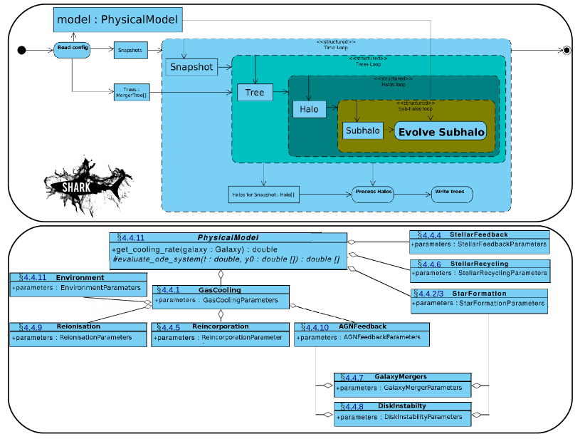
Figure 1: Top panel: Design of Shark. The physical model is the set of ODEs that are solved numerically by Shark (described in $\S$ 4.4.13 for the current Shark model). The implementation of the physical model is detached from the main evolution loop, which allows the code a lot of flexibility to change the description of the interplay between mass, metal and angular momentum components. Note that Shark also allows halos at any given snapshot to interact with each other, despite belonging to different merger trees. Bottom panel: zoom into the structure of the physical model. Most of the relevant physical processes in galaxies respond directly to the physical model. The only two important physical models that are called separately are galaxy mergers and disk instabilities only due to computational expense and simplicity of the code. The classes of AGN feedback and star formation are also linked with those of galaxy mergers and disk instabilities as in these two processes we expect black holes to grow and central starbursts to be driven. We show next to each physical process the section in this paper where we describe the details of the modelling.

Following the same principle, the individual physical processes that participate in the physical model are not hard-wired to the physical model itself, but implemented as independent classes and provided as inputs to the physical model. These classes implement only the logic associated to the particular physical process they represent, exposing it to its callers. If available, different implementations of the same physical process can also be chosen at runtime.

3.2 Scalability

Shark scales naturally with its input data. Input volumes are usually divided into independent sub-volumes that can be individually processed. On the other hand a single Shark execution can be commanded to process one or more sub-volumes. This simple but flexible scheme allows for easy parallelisation based on input data, where multiple Shark executions can be run to process a large number of sub-volumes in parallel. This strategy does not require communication between executions, reducing both the complexity of the software and its dependencies.

Depending on the size of its inputs, Shark will usually be limited by the amount of available memory. Memory usually scales with the number of CPUs, and therefore Shark will usually have multiple CPUs at its disposal. We take advantage of this by further parallelising the execution of Shark using OpenMP. During the main evolution loop, and for any snapshot, the evolution of galaxies belonging to different merger trees is independent from each other. This the place in the code in which most of the time is spent, and thus we parallelise the evolution of individual merger trees so they take place in different threads. The number of threads to use is specified on the command-line, and can be set to either a fixed number, or to the default value provided by the OpenMP library. In addition to this other parts of the code use OpenMP to parallelise their execution.

In some important physical applications, for example to model the epoch of reionisation, halos belonging to different merger trees need to interact with each other (Mutch et al., 2016). This in principle can be implemented in Shark, but in that case the user should run without OpenMP.

3.3 High Performance Computing environments

Shark can also be efficiently and easily run in HPC environments. Shark comes with a shark-submit script to spawn multiple Shark instances to an HPC cluster running over a set of sub-volumes and using a common configuration. The script abstracts away the details of the underlying queueing system and takes care of using all resources optimally (in terms of memory and CPUs), while offering users flexibility over the submission parameters. The script also creates well-organized, per-submission outputs, making it easy to inspect them independently. At the moment of writing only SLURM is supported, but support for Torque/PBS will follow, and more could be added in the future if required.

3.4 Diagnostic plots

Shark includes a set of python scripts (robust under python 2.7 and 3), which produce all the plots in this paper plus several other diagnostic plots. These scripts can be run automatically using shark-submit.

4 Shark physics

In this section we provide a description of the physics included in Shark, showing how the different models are referred to as in the code.

4.1 Evolving galaxies through merger trees

The merger trees and subhalo catalogue of VELOCIraptor+TreeFrog provide a static skeleton within which we need to evolve galaxies. In Shark we make a postprocessing treatment of these merger trees before forming and evolving galaxies across the skeleton, described below.

• Interpolating halos/subhalos. Because TreeFrog searches for primary links up to $4$ snapshots in the future, it can happen that a subhalo has as a descendant subhalo that is not necessarily at the next snapshot. This causes discontinuities at the moment of evolving galaxies. Thus, in Shark we place subhalos between the snapshots of the current subhalo and its descendant, which we term ‘interpolated’ subhalos. The properties of these interpolated subhalos are frozen to those of their progenitor subhalo. This measure ensures continuity to solve the equations of galaxy formation that we detail in $\S$ 4.4. It happens commonly with all available merger tree builders we are aware of, that subhalos disappear from the merger tree (i.e. have no identified descendant). In Shark one can choose to ignore those in the calculation by setting the execution parameter skip_-missing_-descendants to true.

• Ensuring mass growth of halos. Once merger trees are constructed, we navigate them to ensure that the mass of a halo is strictly equal or larger than the halo mass of its most massive progenitor. This is done to ensure that matter accretion onto halos is always $\geq 0$. $\S$ 4.3 describes how the gas accretion rate onto halos is calculated. Other SAMs follow a similar procedure (Lacey et al., 2016), but with the aim of giving the user control over these decisions, Shark includes a boolean parameter, ensure_-mass_-growth, which should be set to false if the user does not wish to include this step. In that case, the negative accretion rates are ignored and set to $0$. Note that Galacticus (Benson, 2012) also allows for these two options. In Shark, we find the results to be very mildly affected by this step due to VELOCIraptor+TreeFrog providing high quality identifications and links that need little additional processing (Poulton et al. submitted).

• Defining the central subhalo. In order to define the central subhalo of every halo in the catalogue, we step at $z=0$ and define the most massive subhalo of every existing halo as the central one. We subsequently make the main progenitor of those centrals as the centrals of their respective halo. We do this iteratively back in time. At every snapshot we find those halos that merge into another, and are not the main progenitors, and apply the same logic described above to designate their central subhalo.

Every subhalo/halo connects to its progenitor(s) and descendant subhalo/halo, which connect to the merger tree in which they have lived throughout their existence. Halos also point to their central subhalo and its satellite subhalos. Every subhalo points to the list of galaxies it may contain, but only central subhalos are allowed to have a central galaxy (which in turn is the central galaxy of the host halo).

The merger trees are a static skeleton and we treat them as such in Shark. Thus, in order to form galaxies and subsequently evolve them, we identify all the halos that first appear in the catalogue (those with no progenitors) and initialize the galaxy pointer, so far composed of one galaxy with zero mass. The central subhalo of that halo is assigned a halo gas reservoir of mass $\Omega_{\rm b}/\Omega_{\rm m}\times M_{\rm halo}$. Having a halo gas mass $>0$ ignites gas cooling and the subsequent formation of a cold gas disk (as detailed in $\S$ 4.4). At the end of every snapshot, we transfer all the galaxies that are hosted by any one subhalo to its descendant and proceed to evolve them. If subhalos appear for the first time in the merger tree as a satellite subhalo, and with the design above, it is defined as a dark subhalo with no allowed to form there.

Shark galaxies exist in $3$ different types: $\tt type=0$ is the central galaxy of the central subhalo, while every other central galaxy of satellite subhalos are $\tt type=1$. If a subhalo merges onto another one and it is not the main progenitor, its given as defunct. All the galaxies of defunct subhalos are made $\tt type=2$ and transferred to the central subhalo of their descendant host halo. Galaxies $\tt type=2$ are widely referred to as ‘orphan galaxies’ (Guo et al., 2016). Note that satellite subhalos can have subhalos themselves (i.e. subsubhalos), and VELOCIraptor+TreeFrog allow for several levels of hierarchy in the subhalo population. However, in Shark all satellite subhalos are treated the same way (as containing satellite galaxies $\tt type=1$) regardless of their hierarchy. In this logic, central subhalos can have one central galaxy and any number of $\tt type=2$ galaxies, while satellite subhalos can only have one $\tt type=1$ galaxy. Any $\tt type=2$ galaxies a subhalo can have before becoming satellite, are transferred to the central subhalo once it becomes a satellite subhalo.

Table 2 lists the execution parameters in Shark with their possible values and those adopted by default. The parameter, ode_-solver_-precision, determines the numerical precision to which the user wishes to solve the set of ODEs of $\S$ 4.4.13.

Table 2: Shark execution parameters. Here we show the names these variables have in the code and the values chosen for our default Shark model in parenthesis in the middle column.

Execution parameter	suggested value range
ensure-mass-growth	true or false (true)
skip-missing-descendants	true or false (true)
ode-solver-precision	$10^{-3}-0.1$ ($0.05$)

4.2 Dark matter halos

When halos are formed, we assume them to have virial radii $r_{\rm vir}=(3M_{\rm halo}/(4\pi\Delta_{\rm vir}\rho_{\rm crit}))^{1/3}$, where $M_{\rm halo}$ is the halo mass, $\rho_{\rm crit}$ is the cosmological critical density at that redshift, and the overdensity $\Delta_{\rm vir}(\Omega_{m},\Omega_{v})=200$. Based on the spherical collapse model, Cole & Lacey (1996) estimated $\Delta_{\rm vir}(\Omega_{m},\Omega_{v})=178$, but a more widely adopted value based on $N$-body simulations is $200$. We assume DM halos to have a density profile that follow a NFW profile:

$$\rho_{\rm DM}(r)\propto\frac{1}{(r/r_{\rm s})(1+r/r_{\rm s})^{2}},$$ (1)

where $r_{\rm s}$ is the scale radius, related to the virial radius by the concentration, $r_{\rm s}=r_{\rm vir}/c_{\rm NFW}$. In Shark we estimate concentrations using the Duffy et al. (2008) relation between concentration, halo’s virial mass and redshift. The user can choose to do this using instea the relation of Dutton & Macciò (2014). The latter is controlled by the input parameter concentration_-model.

Halos grow via merging with other halos and by accretion. The properties $r_{\rm vir}$ and $M_{\rm halo}$ are calculated by VELOCIraptor at each snapshot. In addition, the user can choose to either use the input halo’s spin parameter, $\lambda_{\rm DM}$, calculated in VELOCIraptor (which corresponds to the Bullock et al. 2001 spin parameter), or draw it from a log-normal distribution of mean $0.03$ and width $0.5$. This is controlled by the boolean parameter ${\tt lambda_{-}random}$. The halo’s angular momentum is then calculated from the mass and halo’s spin parameters, adopting Mo et al. (1998),

$$J_{\rm h}=\frac{\sqrt{2}\,G^{2/3}}{(10\,H(z))^{1/3}}\lambda_{\rm DM}\,M^{5/3}_{\rm h},$$ (2)

where $G$ is Newton’s gravity constant and $H(z)$ is the Hubble parameter. In the future we plan to add additional plausible profiles (e.g. Einasto 1965) for the users to decide which one they prefer.

4.3 Matter accretion onto halos

When halos are first formed, we assume that a fraction $\Omega_{\rm b}$ is in the form of hot halo gas with a temperature $T_{\rm vir}=(\mu m_{\rm H}/2k_{\rm B})v_{\rm vir}^{2}$, where $v_{\rm vir}=(G\,M_{\rm halo}/r_{\rm vir})^{1/2}$, and $\mu$ is the mean molecular weight. We assume that this gas has a minimum fraction of metals $Z_{\rm min}$.

Any subsequent gas accretion onto the halos from the cosmic web is calculated based on the DM mass a halo gains that does not come via mergers. We do this by adding up all the mass contributed by the progenitor halos, and taking the difference with the halo mass at the current timestep, $\Delta M=M_{\rm halo,curr}-M_{\rm halo,prog}$. Contreras et al. (2017) showed that halos can have sudden changes in their mass due to misidentification by halo/subhalo finders and by the construction of the merger tree. Analysing several snapshots to clean the subhalo catalogues as is done in several algorithms (Behroozi et al., 2013b; Jiang et al., 2014; Elahi et al., 2018), helps to avoid this problem, but to some extent it can still be present. In order to avoid these sudden changes in mass to have a big effect on the accretion rates calculated here and introduce systematic problems, we limit the maximum baryon mass halos can have to the universal baryon fraction, with baryons here including galaxy masses, halo gas and ejected gas. The latter is not strictly within halos, but makes up the intergalactic medium, which is formed by the effect of outflows (details presented in $\S$ 4.4.4 and 4.4.5). We assume that the accreted matter brings a fraction $\Omega_{\rm b}$ of baryons with a metallicity $Z_{\rm min}$. Bromm & Larson (2004) argue that population III stars can lead to a nearly uniform enrichment of the universe to a level of $Z~{}10^{-4}\rm\,Z_{\odot}$, and thus $Z_{\rm min}$ would typically take a value close to that.

4.4 Physical modelling of galaxy formation and evolution

In Shark we include a large library of physical models describing gas cooling, star formation, stellar feedback and chemical enrichment, BH growth, AGN feebdack, galaxy mergers, disk instabilities, the development of galaxy sizes and environmental effects. Each of these mechanisms can be modelled in different ways, so Shark includes several different models for any one physical process. One of the missions of Shark is to be constantly updating the code to include more plausible models for all the different physical processes above, and possibly to add additional physical processes over time.

Below we describe the models that are included in v1.1. At the end of this section we present all the parameters and models that can be included in Shark in Tables 3 and 4, together with suggested ranges of values, and the values adopted in our default model.

4.4.1 Gas in halos and cooling

Gas in halos are assumed in Shark to have two phases: cold and hot. Cold halo gas is the gas that cools down within a simulation snapshot, while the hot halo gas corresponds to the gas that is at the virial temperature and that has not had time to cool down yet. The halo gas settles into a spherically symmetric distribution with some density profile. We implement an isothermal profile,

$$\rho_{\rm g}(r)=\frac{m_{\rm gas,h}}{4\pi\,r^{2}_{\rm vir}\,r},$$ (3)

where $m_{\rm gas,h}$ is the total halo gas.

This halo gas then loses its thermal energy by radiative cooling due to atomic processes, at a rate per unit volume $\rho^{2}_{\rm g}\Lambda(T_{\rm vir},z_{\rm gas,h})$, in which collisional ionization equilibrium is assumed, and where $z_{\rm gas,h}$ is the metallicity of this gas. We use CLOUDY version 08 (Ferland et al., 1998) to produce tabulated cooling functions in a grid of $(T_{\rm vir},z_{\rm gas,h})$, assuming collisional ionization equilibrium and without considering the effects of dust. Alternatively, the user can also choose to use instead the cooling tables of Sutherland & Dopita (1993). We interpolate over this large grid at each snapshot for each halo to estimate $\Lambda$. Note that Shark uses the cooling rate to solve the ODEs of Eqs. 53-68, and therefore it is not very sensitive to the simulation snapshots, even though the cold halo gas mass is.

The cooling time is related to the density as

$$t_{\rm cool}(r)=\frac{3}{2}\frac{\mu m_{\rm H}\,\kappa_{\rm B}\,T_{\rm vir}}{\rho_{\rm g}(r)\,\Lambda(T_{\rm vir},z_{\rm gas,h})},$$ (4)

where $\kappa_{\rm B}$ is Boltzmann’s constant. The cooled gas corresponds to that enclosed within the cooling radius, $r_{\rm cool}$. We refer to that gas as cold halo gas. In v1.1, we calculate the cooling time and radius by employing two different models, Benson & Bower (2010) and Croton et al. (2006). These two modes take different approaches to estimate the cooling time, which is then used to estimate $r_{\rm cool}$. Below we summarize these two approaches.

• The Croton06 model. Croton et al. (2006), also adopted by Guo et al. (2011) and Henriques et al. (2015), assume that the cooling time, $t_{\rm cool}$, at the cooling radius is of a similar magnitude to the dynamical timescale, and simply calculates it as $t_{\rm cool}\equiv r_{\rm vir}/v_{\rm vir}$. Croton et al. (2006) then derive $r_{\rm cool}$ from Eq. 4. The cooling rate is then calculated from the continuity equation

  $$\dot{m}_{\rm cool}=4\pi\,\rho_{\rm g}(r_{\rm cool})\,r^{2}_{\rm cool}\dot{r}_{\rm cool}.$$ (5)

  This is valid only if $r_{\rm cool}<r_{\rm vir}$ (referred to as ‘hot-halo mode’). In the case $r_{\rm cool}>r_{\rm vir}$, all the halo gas is accreted onto the galaxy in a dynamical timescale (referred to as ‘cold-halo mode’).

• The Benson10 model. Benson & Bower (2010) define a time available for cooling. In the case of an static halo, this time available for cooling is equivalent to the time since the halo came into existence. Benson & Bower (2010) assume $t_{\rm cool}\equiv t_{\rm avail}$, where

  $$t_{\rm avail}=\frac{\int_{0}^{t}\,[T_{\rm v}(t^{\prime})\,M_{\rm gas,h}(t^{\prime})/t_{\rm cool}(t^{\prime})]\,{\rm d}t^{\prime}}{T_{\rm v}(t)\,M_{\rm gas,h}(t)/t_{\rm cool}(t)},$$ (6)

  with $t$ corresponding to the current time. The cooling time above is computed at the mean density of the notional profile, $\rho_{\rm g}$. Having computed $t_{\rm avail}$ we solve for $r_{\rm cool}$ by $t_{\rm cool}(r_{\rm cool})=t_{\rm avail}$. The current infall radius, $r_{\rm infall}$, is then taken to be the smaller of the cooling and freefall radii. The cooled mass that is accreted onto the galaxy is simply that enclosed by $r_{\rm infall}$.

In summary, the main difference between the Croton06 and Benson10 models, is what they assume for the time available for cooling. Which in the former, it is assumed to be equal to the dynamical time of the halo. The adopted model for cooling can be seen as ‘adjustable parameters’ in the sense that using one or the other can change the predicted galaxy population. The distinction between ‘cold’ and ‘hot’ halo gas is reset at every snapshot, and is used when solving the ODEs described in Eqs. 53-68.

4.4.2 Star formation in disks

The gas is assumed to follow an exponential profile of half-mass radius $r_{\rm gas,disk}$ (see $\S$ 4.4.12 for a definition). We calculate the SFR surface density assuming a constant depletion time for the molecular gas,

$$\Sigma_{\rm SFR}=\nu_{\rm SF}\,f_{\rm mol}\,\Sigma_{\rm gas},$$ (7)

where $\nu_{\rm SF}$ is the inverse of the H₂ depletion timescale, and $f_{\rm mol}\equiv\Sigma_{\rm mol}/\Sigma_{\rm gas}$, where $\Sigma_{\rm mol}$ is the molecular gas surface density and $\Sigma_{\rm gas}$ is the total gas surface density. Below we provide details on how we estimate $f_{\rm mol}$. Some of the models included in Shark calculate a $\nu_{\rm SF}$ that depends on galaxy properties, while other models assume the observational value $\nu_{\rm SF}=1/\tau_{\rm H_{2}}$, with $\tau_{\rm H_{2}}=2.2^{+2.1}_{-1.1}\,\rm Gyr$ (Leroy et al., 2013) being the observed molecular gas depletion timescale. The latter is the case for the BR06 and GD14 models.

The HI surface densities cannot extend to infinitely small surface densities because the UV background can easily ionise very low density gas. Thus, we impose a limit in the minimum HI density allowed before the gas becomes ionised, $\Sigma_{\rm thresh}$, and adopt $\Sigma_{\rm thresh}=0.1\,\rm M_{\odot}\,pc^{-2}$ following the results of the hydrodynamical simulations of Gnedin (2012). In reality this threshold should evolve with redshift, increasing at earlier epochs when the UV background is brighter (Haardt & Madau, 2012).

We integrate $\Sigma_{\rm SFR}$ over the radii range $0-10\rm r_{\rm gas,disk}$ to obtain the instantaneous SFR, $\psi$. We do this using an adaptive integrator that adopts a 15 point Gauss-Kronrod rule (due to its speed), available in the GSL C++ libraries. We enforce a $1$% accuracy.

Shark has several implementations to calculate $f_{\rm mol}$, which are described below.

• The BR06 model. Blitz & Rosolowsky (2006) found that the H₂ to HI ratio, $R_{\rm mol}\equiv\Sigma_{\rm H_{2}}/\Sigma_{\rm HI}$, correlates with the local hydrostatic pressure as

  $$R_{\rm mol}=\left(\frac{P}{P_{0}}\right)^{\alpha_{P}},$$ (8)

  where $P_{0}$ and $\alpha_{P}$ are parameters measured in observations and have values $P_{0}/\kappa_{\rm B}=1,500-40,000\,\rm cm^{-3}\,\rm K$ and $\alpha_{P}\approx 0.7-1$ (Blitz & Rosolowsky, 2006; Leroy et al., 2008, 2013). We calculate the hydrostatic pressure from the surface densities of gas and stars following Elmegreen (1989),

  $$P=\frac{\pi}{2}\,G\,\Sigma_{\rm gas}(\Sigma_{\rm gas}+\frac{\sigma_{\rm gas}}{\sigma_{\star}}\,\Sigma_{\star}),$$ (9)

  where $\Sigma_{\rm gas}$ and $\Sigma_{\star}$ are the total gas (atomic plus molecular) and stellar surface densities, respectively, and $\sigma_{\rm gas}$ and $\sigma_{\star}$ are the gas and stellar velocity dispersions. The stellar surface density is assumed to follow an exponential profile with a half-mass stellar radius of $r_{\star,\rm disk}$. We adopt $\sigma_{\rm gas}=10\,\rm km\,s^{-1}$ (Leroy et al., 2008) and calculate $\sigma_{\star}=\sqrt{\pi\,G\,h_{\star}\,\Sigma_{\star}}$. Note that $\sigma_{\rm gas}$ is treated as a free parameter in the sense that the user can set it to different values, though we recommend to adopt values that do not deviate much from the observational measurement. Here, $h_{\star}$ is the stellar scale height, and we adopt the observed relation $h_{\star}=r_{\star}/7.3$ (Kregel et al., 2002), with $r_{\star}$ being the half-stellar mass radius (see $\S$ 4.4.12).

• The GD14 model. Gnedin & Draine (2014) presented the results of cosmological hydrodynamical simulations that include the formation of H₂. These simulations also included gravity, hydrodynamics, non-equilibrium chemistry combined with equilibrium cooling rates for metals, and a 3-dimensional, on the fly, treatment of radiative transfer, using an Adaptive Mesh Refinement (AMR) code. Compared to earlier implementations (Gnedin & Kravtsov, 2011), Gnedin & Draine (2014) paid special attention to the effect of line overlap in the Lyman and Werner bands in H₂ shielding. Gnedin & Draine (2014) presented a model for $R_{\rm mol}$ that describes the simulation results well. This model depends on the dust-to-gas ratio, $D_{\rm MW}$, and the local radiation field, $U_{\rm MW}$, with respect to that of the solar neighbourhood (i.e. they therefore are dimensionless parameters). We estimate these two parameters as $D_{\rm MW}=Z_{\rm gas}/Z_{\odot}$ and $U_{\rm MW}=\Sigma_{\rm gas}/\Sigma_{\rm MW}$, where $Z_{\rm gas}$ is the metallicity of the ISM. We adopt $Z_{\odot}=0.134$ (Asplund et al., 2009) and $\Sigma_{\rm MW}=2.5\,\rm M_{\odot}\,yr^{-1}$ (Bonatto & Bica, 2011).

  The approximation we use for $U_{\rm MW}$ is based on the argument of Wolfire et al. (2003) that pressure balance between the warm and the cold neutral media is achieved only if the density is larger than a minimum density, which is proportional to $U_{\rm MW}$. Thus, if we assume that pressure equilibrium between the warm/cold media is a requirement for the formation of the ISM, we can then assume that $U_{\rm MW}\propto\rho_{\rm gas}$, with $\rho_{\rm gas}$ being the gas density. Since galaxies show a close to constant $\sigma_{\rm gas}$, we can assume that the gas scale height is close to constant, which allow us to replace $\rho_{\rm gas}$ by $\Sigma_{\rm gas}$ above.

  Based on $D_{\rm MW}$ and $U_{\rm MW}$ we calculate $R_{\rm mol}$ following Gnedin & Draine (2014),

  $$R_{\rm mol}=\left(\frac{\Sigma_{\rm gas}}{\Sigma_{\rm R=1}}\right)^{\alpha_{\rm GD}},$$ (10)

  where

  $$\alpha_{\rm GD}=0.5+\frac{1}{1+\sqrt{U_{\rm MW}D^{2}_{\rm MW}/600}},$$ (11)

  $$\Sigma_{\rm R=1}=\frac{50\,\rm M_{\odot}\,pc^{-2}}{g}\,\frac{\sqrt{0.01+U_{\rm MW}}}{1+0.69\sqrt{0.01+U_{\rm MW}}},$$ (12)

  and

  $$g=\sqrt{D^{2}_{\rm MW}+D^{2}_{\star}}.$$ (13)

  Here, $D_{\star}\approx 0.17$ for scales $>500\,\rm pc$.

• The KMT09 model. Krumholz et al. (2009), hereafter KMT09, calculated $\nu_{\rm SF}$ and $f_{\rm mol}$ in Eq. 7 for a spherical cloud with SF regulated by supersonic turbulence. KMT09 assume that $f_{\rm mol}$ is determined by the balance between the photodissociation of H₂ molecules by the interstellar far-UV radiation and the formation of molecules on the surface of dust grains, and calculated it theoretically to be a function of the total gas surface density of the cloud and of the gas metallicity (see Eq. $2$ in KMT09). The gas surface density of the cloud is related to the disk gas surface density via a cumpling factor, $f_{\rm c}$. The latter is argued to be $f_{\rm c}\approx 5$ when averaging over $1$ kpc region in local galaxy disks. KMT09 estimated $\nu_{\rm SF}$ from the theoretical model of turbulent fragmentation of Krumholz & McKee (2005). In this model, $\nu_{\rm SF}$ depends on the cloud surface density, which in spiral galaxies is assumed to be constant, with an observed value of $\Sigma_{0}\approx 85\,\rm M_{\odot}\,\rm pc^{-2}$. In starbursts (SBs), however, the ambient pressure is expected to increase significantly, which is accompanied by gas surface densities that can become larger than $\Sigma_{0}$. KMT09 argue that clouds will therefore have a density $\Sigma_{\rm cl}={\rm max}[\Sigma_{0},\Sigma_{\rm gas}]$, which leads to $\nu_{\rm SF}$ to be described as

  $$\nu_{\rm SF}=\left\{\begin{array}[]{rl}\nu^{0}_{\rm SF}\,\left(\frac{\Sigma_{\rm gas}}{\Sigma_{0}}\right)^{-0.33},&\mbox{$\Sigma_{\rm gas}<\Sigma_{0},$}\\ \nu^{0}_{\rm SF}\,\left(\frac{\Sigma_{\rm gas}}{\Sigma_{0}}\right)^{0.33},&\mbox{ $\Sigma_{\rm gas}\geq\Sigma_{0}.$}\end{array}\right.$$ (16)

• The K13 model. Krumholz (2013) developed a theoretical model for the transition from HI-to-H₂ that depends on the total column density of neutral hydrogen, the gas metallicity and the interstellar radiation field. A key property in the Krumholz (2013) model is the density of the cold neutral medium (CNM). At densities $n_{\rm H}\gtrsim 0.5\,\rm cm^{-3}$, the transition from HI to H₂ is mainly determined by the minimum density that the CNM must have to ensure pressure balance with the warm neutral medium (WNM, which is HI dominated). The assumption is that the CNM is supported by turbulence, while the WNM is thermally supported (see also Wolfire et al. 2003). At $n_{\rm H}\lesssim 0.5\,\rm cm^{-3}$ the transition from HI to H₂ is mainly determined by the hydrostatic pressure, which has three components: the self-gravity of the WNM ($\propto\Sigma^{2}_{\rm HI}$), the gravity between the CNM and WNM ($\propto\Sigma_{\rm HI}\Sigma_{\rm H_{2}}$), and the gravity between the WNM and the stellar plus DM component ($\propto\Sigma_{\rm HI}\Sigma_{\rm sd}$, where $\Sigma_{\rm sd}$ is the surface density of stars plus DM). Note that the exact value of $n_{\rm H}$ at which the transition between these two regimes takes place is a strong function of gas metallicity. For this model, we adopt the same dust-to-gas mass ratio and local radiation field as in the GD14 model. We then define two densities, one that corresponds to the CNM density in the regime of two-phase equilibrium, $n_{\rm CNM,2p}$, and the CNM density set by hydrostatic balance, $n_{\rm CNM,hydro}$. The former (latter) is expected to dominate at high (low) gas surface densities. These densities are defined as:

  $$n_{\rm CNM,2p}\approx 23\,U_{\rm MW}\,\left(\frac{1+3.1\,D^{0.365}_{\rm MW}}{4.1}\right)^{-1}\,{\rm cm}^{-3},$$ (17)

  and

  $$n_{\rm CNM,hydro}=\frac{P_{\rm th}}{1.1\,k_{\rm B}\,T_{\rm CNM,max}},$$ (18)

  where $T_{\rm CNM,max}$ is the maximum temperature at which the CNM can exist ($\approx 243$ K; Wolfire et al. 2003), and

  $$P_{\rm th}\approx\frac{\pi\,G\,\Sigma^{2}_{\rm gas}}{4\,\alpha}\left[1+\sqrt{1+\frac{32\,\zeta_{\rm d}\,\alpha\,f_{\rm w}\,\sigma^{2}_{\rm gas}\,\rho_{\rm sd}}{\pi\,G\,\Sigma^{2}_{\rm gas}}}\right].$$ (19)

  Here $\alpha\approx 5$ represents how much of the midplane pressure support comes from turbulence, magnetic fields and cosmic rays, compared to the thermal pressure (Ostriker et al., 2010), $\zeta_{\rm d}\approx 0.33$ is a numerical factor that depends on the shape of the gas surface isodensity contour, $f_{\rm w}=0.5$ is the ratio between the mass-weighted mean square thermal velocity dispersion and the square of the sound speed of the warm gas (the value adopted here originally comes from Ostriker et al. 2010) and $f_{\rm c}$ is the clumping factor (as in KMT09). The value of the gas density in the CNM is then taken to be $n_{\rm CNM}={\rm max}(n_{\rm CNM,2p},n_{\rm CNM,hydro})$.

  K13 defines a dimensionless radiation field parameter:

  $$\chi=7.2\,U_{\rm MW}\left(\frac{n_{\rm CNM}}{10\,{\rm cm}^{-3}}\right)^{-1},$$ (20)

  and writes $f_{\rm mol}$ as

  $$f_{\rm H_{2}}=\left\{\begin{array}[]{rl}1-{0.75\,s}/({1+0.25\,s}),&\mbox{ $s<2$,}\\ 0,&\mbox{ $s\geq 2,$}\end{array}\right.$$ (23)

  where

  $$s \approx \frac{{\rm ln}(1+0.6\,\chi+0.01\,\chi^{2})}{0.6\,\tau_{\rm c}},$$ (24)

  $$\tau_{\rm c} = 0.066\,f_{\rm c}\,D_{\rm MW}\,\left(\frac{\Sigma_{\rm gas}}{\rm M_{\odot}{\rm pc}^{-2}}\right).$$ (25)

  We use Eq. 16 to estimate $\nu_{\rm SF}$ for this model.

4.4.3 Star formation in bulges

SBs, which can be triggered by either galaxy mergers or disk instabilities, build up the central bulge in Shark. Thus, when we refer to SBs, we mean star formation taking place in the central bulge.

There is strong evidence that SBs follow a similar relation to normal star-forming galaxies studied in Leroy et al. (2013) but with a timescale significantly shorter (Daddi et al., 2010b; Genzel et al., 2015; Tacconi et al., 2018). We then adopt the same calculation of $R_{\rm mol}$, $\Sigma_{\rm gas}$ and $P$ above for bulges, replacing the disk properties with the bulge’s. The only important difference is that we apply a boost factor to the star formation efficiency $\nu_{\rm SF,burst}=\eta_{burst}\nu_{\rm SF}$, with $\eta_{burst}$ taking values in the range $\approx 1-10$, according to observations (Daddi et al., 2010b; Scoville et al., 2016; Tacconi et al., 2018).

We implicitly assume that the gas in the bulge also settles in an exponential disk with scale length $r_{\rm bulge}/1.67$. To avoid calculating SFRs for very small quantities of gas left in the bulges, we decide to transfer the bulge gas to disk if it drops below $\rm min_{\rm gas,bulge}$. We find that for the resolution of the L210N1504, our default option, values $<10^{5.5}\rm\,M_{\odot}$ gives the same results. Our default option is $\rm min_{\rm gas,bulge}=10^{5}\rm\,M_{\odot}$.

4.4.4 Stellar feedback

Shark separates stellar feedback into two main components: the outflow rate of the gas that escapes from the galaxy, $\dot{m}_{\rm outflow}$, and the ejection rate of the gas that escapes from the halo, $\dot{m}_{\rm ejected}$. We implement different descriptions of SNe feedback, but $\dot{m}_{\rm outflow}$ and $\dot{m}_{\rm ejected}$ are related in the same way in all the model variants.

We can describe $\dot{m}_{\rm outflow}=\psi\,{\rm f}(z,V_{\rm circ})$, where $\psi$ is the instantaneous SFR, $z$ is the redshift and $V_{\rm circ}$ is the maximum circular velocity of the galaxy. The ejection rate of the halo should be $>0$ only in the case where the injected total energy of the outflow is larger than the specific binding energy of the halo. Muratov et al. (2015) used the FIRE simulation suite to estimate several properties of the stellar driven outflows, including the terminal wind velocity, $V_{\rm w}$. Muratov et al. (2015) found that

$$\frac{V_{\rm w}}{\rm km\,s^{-1}}=1.9\,\left(\frac{V_{\rm circ}}{\rm km\,s^{-1}}\right)^{1.1}.$$ (26)

We use this terminal velocity to compute the excess energy that will be used to eject gas out of the halo as

$${\rm E}_{\rm excess}=\epsilon_{\rm halo}\,\frac{V^{2}_{\rm w}}{2}\psi\,{\rm f}(z,V_{\rm circ}).$$ (27)

Here $\epsilon_{\rm halo}$ is a free parameter. The net ejection rate is therefore calculated as,

$$\dot{m}_{\rm ejected}=\frac{{\rm E}_{\rm excess}}{V^{2}_{\rm circ}/2}-\dot{m}_{\rm outflow}.$$ (28)

If $\dot{m}_{\rm ejected}<0$ no ejection from the halo takes place and we limit $\dot{m}_{\rm outflow}={\rm E}_{\rm excess}/(V^{2}_{\rm circ}/2)$.

As discussed above we implemented several models for ${\rm f}(z,V_{\rm circ})$, described below.

• The Lacey16 model. Bower et al. (2012) presented a version of GALFORM that distinguishes the components $\dot{m}_{\rm outflow}$ and $\dot{m}_{\rm ejected}$, describing the function $f$ in a very simple fashion as,

  $${\rm f}=\left(\frac{V_{\rm circ}}{v_{\rm hot}}\right)^{\beta},$$ (29)

  with $\beta<0$. Here there is no redshift dependence. In the Bower et al. (2012) model $\beta=-3.2$ and $v_{\rm hot}=350\,\rm km\,s^{-1}$. Note that in the standard GALFORM implementation of Lacey et al. (2016), $\dot{m}_{\rm ejected}\equiv\dot{m}_{\rm outflow}$, and thus, in Shark we also enforce that equivalency.

• The Guo11 model. Guo et al. (2011) described SNe feedback as

  $${\rm f}=\epsilon_{\rm disk}\,\left[0.5+\left(\frac{V_{\rm circ}}{v_{\rm hot}}\right)^{\beta}\right].$$ (30)

  Guo et al. (2011) adopted $v_{\rm hot}=70\,\rm km\,s^{-1}$, $\beta=-3.5$ and $\epsilon_{\rm disk}=6.5$, all of which were adjusted to fit the stellar mass function.

• The Muratov15 model. Muratov et al. (2015) presented a detailed analysis of the stellar driven outflows produced in the FIRE simulation suite by tracking explicitly the SPH particles and using kinematics to distinguish between outflowing and inflowing gas. Muratov et al. (2015) found that the outflow rates relative to $\psi$ (also termed ‘mass loading’) evolved significantly with redshift. They provide a best fit to the scaling between $\dot{m}_{\rm outflow}$ and $\psi$, z, $V_{\rm circ}$ as

  $${\rm f}=\epsilon_{\rm disk}\,(1+z)^{\rm z_{\rm P}}\,\left(\frac{V_{\rm circ}}{v_{\rm hot}}\right)^{\beta},$$ (31)

  with $\epsilon_{\rm disk}=2.9$, $\rm z_{\rm P}=1.3$, $v_{\rm hot}=60\,\rm km\,s^{-1}$ and $\beta=-3.2$ if $V_{\rm circ}<v_{\rm hot}$ and $\beta=-1$ if $V_{\rm circ}>v_{\rm hot}$. The redshift scaling in FIRE implies $L^{*}$ galaxies have mass loadings of $\approx 10$ at $z=6$ and $<1$ at $z=0$.

• The Lagos13 model. Lagos et al. (2013) presented a detailed modelling of the expansion of SNe driven bubbles in a two-phase ISM. The authors followed the evolution of these bubbles from the early epoch of adiabatic expansion, to the momentum driven expansion until either confinement in the disk or break-out from the disk. They used this model to estimate $\dot{m}_{\rm outflow}$ and find

  $${\rm f} = \epsilon_{\rm disk}\,\left(\frac{V_{\rm circ}}{v^{\prime}_{\rm hot}}\right)^{\beta},$$ (32)

  $$v^{\prime}_{\rm hot} = v_{\rm hot}\,(1+z)^{\rm z_{\rm P}},$$ (33)

  Lagos et al. (2013) found values of $v_{\rm hot}=425\,\rm km\,s^{-1}$, $\beta=2.7$, $\rm z_{\rm P}=-0.2$, $\epsilon_{\rm disk}=1$. Note that Lagos et al. (2013) found that the mass loading decreases with increasing redshift in tension with the findings of Muratov et al. (2015). This discrepancy is not necessarily due to the Lagos et al. model being a simpler description of the stellar feedback process, which is evidenced by previous hydrodynamical simulations (e.g. Creasey et al. 2013; Hopkins et al. 2012b) finding results similar to those in Lagos et al. (2013). This is clearly a controversial topic and thus justifies our decision of implementing several different models of stellar feedback and leaving the parameters to vary. Note that assuming $\rm z_{\rm P}>0$ in Eq. 33 mimics the effect reported in Muratov et al. (2015). In fact, in our default Shark model, we adopt the Lagos13 model but with $\rm z_{\rm P}>0$.

We also allow for two variants of the Lacey16 and Lagos13 models. In the case of the former, we implement a redshift dependence with the same form as in Eq. 33. We refer to this variant as Lacey16RedDep. For Lagos13 we also apply a variant that reproduces the break of the Muratov15 mass loading function, implemented such that at $V_{\rm circ}>v_{\rm hot}$, $\beta=-1$. We refer to this model as Lagos13Trunc. Note that Lacey16RedDep is different from Lagos13 in that the former assumes $\dot{m}_{\rm ejected}\equiv\dot{m}_{\rm outflow}$, though $\dot{m}_{\rm outflow}$ would have the same functional form.

4.4.5 Reincorporation of ejected gas

The gas expelled from the halos of galaxies by stellar feedback is assumed to be reincorporated in a timescale that is mass dependent. We follow the method developed by Henriques et al. (2013) and describe the reincorporation rate as

$$\dot{m}_{\rm reinc}=\frac{m_{\rm ejected}}{\tau_{\rm reinc}\,\left(M_{\rm halo}/M_{\rm norm}\right)^{\gamma}}.$$ (34)

Here, $m_{\rm ejected}$ is the reservoir of ejected mass, $\tau_{\rm reinc}$, $M_{\rm norm}$ and $\gamma$ are free parameters. Henriques et al. (2013) found that in their model the best values for these parameters to fit the SMF of galaxies at $z=0$ and $z=2$ simultaneously, were $18\,\rm Gyr$, $10^{10}\,\rm M_{\odot}$ and $-1$, respectively. In Shark, a value $\tau_{\rm reinc}=0$ is interpreted as the user adopting instantaneous reincorporation.

4.4.6 Recycled fraction and yield

For chemical enrichment in Shark, we adopt the instantaneous recycling approximations for the metals in the ISM. This implies that the metallicity of the ISM gas mass instantaneously absorbs the fraction of recycled mass and newly synthesised metals in recently formed stars, neglecting the time delay for the ejection of gas and metals from stars.

The recycled mass injected back to the ISM by newly born stars is calculated from the initial mass function (IMF) as,

$$R=\int_{m_{\rm min}}^{m_{\rm max}}\,(m-m_{\rm rem})\phi(m)\,{\rm d}m,$$ (35)

where $m_{\rm rem}$ is the remnant mass and the IMF is defined as $\phi(m)\propto dN(m)/dm$. Similarly, we define the yield as

$$p=\int_{m_{\rm min}}^{m_{\rm max}}\,m_{\rm i}(m)\phi(m){\rm d}m,$$ (36)

where $m_{\rm i}(m)$ is the mass of newly synthesised metals ejected by stars of initial mass $m$. The minimum and maximum mass in the integrations are taken to be $m_{\rm min}=1\,M_{\odot}$ and $m_{\rm max}=120\,M_{\odot}$. Stars with masses $m<1\,M_{\odot}$ have lifetimes longer than the age of the Universe, and therefore they do not contribute to the recycled fraction and yield. We use the stellar population model of Conroy et al. (2009) to calculate $m_{\rm rem}$ and $m_{\rm i}(m)$ in Eqs. 35 and 36, respectively.

In Shark we assume the stellar IMF is assumed to be universal and take the shape of a Chabrier (2003) IMF. This is a widely adopted IMF in observations and so it facilitates comparisons. Under this assumption we obtain $p=0.029$ and $R=0.46$. Note that these values are subject to the assumed models for the remnant mass and yields, and therefore are left as ‘free’ parameter. We, however, advice to apply only small perturbations to the values suggested here, unless well informed.

4.4.7 Galaxy mergers

When DM halos merge, we assume that the galaxy hosted by the main progenitor halo (see $\S$ 4.1 for details) becomes the central galaxy, while all the other galaxies become satellites orbiting the central galaxy. These orbits gradually decay towards the centre due to energy and angular momentum losses driven by dynamical friction with the halo material, including other satellites. We distinguish between two types of satellite galaxies as described in $\S$ 4.1. We calculate a dynamical friction timescale for orphan satellites only, and merge those with the central once that clock goes to zero.

Depending on the amount of gas and baryonic mass involved in the galaxy merger, a SB can be triggered. The time for the satellite to hit the central galaxy is called the orbital timescale, $\tau_{\rm merge}$, which is calculated following Lacey & Cole (1993) as

$$\tau_{\rm merge}=f_{\rm df}\,\Theta_{\rm orbit}\,\tau_{\rm dyn}\,\left[\frac{0.3722}{{\rm ln}(\Lambda_{\rm Coulomb})}\right]\,\frac{M}{M_{\rm sat}}.$$ (37)

Here, $f_{\rm df}$ is a dimensionless adjustable parameter which is $f_{\rm df}\leq 1$, $\Theta_{\rm orbit}$ is a function of the orbital parameters, $\tau_{\rm dyn}\equiv R_{\rm v}/V_{\rm v}$ is the dynamical timescale of the halo, ${\rm ln}(\Lambda_{\rm Coulomb})={\rm ln}(M/M_{\rm sat})$ is the Coulomb logarithm, $M$ is the halo mass of the central galaxy and $M_{\rm sat}$ is the mass of the satellite, including the mass of the DM halo in which the galaxy was formed. Note that the parameter $f_{\rm df}$ provides the flexibility to choose to merge galaxies right after the subhalos disappear from the catalogs ($f_{\rm df}=0$). In addition, this parameter may be $>0$ but $<1$ if the subhalos tend to disappear deep into the potential well when their number of particles drop below the threshold imposed by the subhalo finder (which is the ideal case). In this case, the dynamical friction timescales should be a lot shorter than Eq. 37 with $f_{\rm df}=1$, as that was originally calculated for subhalos at the virial radius. Simha & Cole (2017) argued that the true dynamical friction timescale for orphan satellites would be smaller than Eq. 37 with $f_{\rm df}=1$ if satellites are modelled as we do in Shark (i.e. by not allowing type 1 satellites to merge). Thus, we leave $f_{\rm df}$ to vary freely, though we recommend to adopt values between $0$ and $1$.

The orbital function, $\Theta_{\rm orbit}$ is defined as

$$\Theta_{\rm orbit}=\left[\frac{J}{J_{\rm c}(E)}\right]^{0.78}\,\left[\frac{r_{\rm c}(E)}{R_{\rm v}}\right]^{2},$$ (38)

where $J$ is the initial angular momentum and $E$ is the energy of the satellite’s orbit, and $J_{\rm c}(E)$ and $r_{\rm c}(E)$ are the angular momentum and radius of a circular orbit with the same energy as that of the satellite, respectively. Thus, the circularity of the orbit corresponds to $J/J_{\rm c}(E)$. The dependence of $\Theta_{\rm orbit}$ on $J$ in Eq 38 is a fit to numerical simulations (Lacey & Cole, 1993). The function $\Theta_{\rm orbit}$ is well described by a log normal distribution with median value $\langle{\rm log}_{10}\Theta_{\rm orbit}\rangle=-0.14$ and dispersion $\langle({\rm log}_{10}\Theta_{\rm orbit}-\langle{\rm log}_{10}\Theta_{\rm orbit}\rangle)^{2}\rangle^{1/2}=0.26$, and its value is not correlated with satellite galaxy properties. Therefore, for each satellite, the value of $\Theta_{\rm orbit}$ is randomly chosen from the above distribution.

If $\tau_{\rm merge}<t-t_{\rm orphan}$ for a satellite galaxy, with $t_{\rm orphan}$ being the time the galaxy became orphan, we proceed to merge it with the central galaxy at a time $t$. If the total mass of gas plus stars of the primary (largest) and secondary galaxies involved in a merger are $M_{\rm p}=M_{\rm cold,p}+M_{\star,\rm p}$ and $M_{\rm s}=M_{\rm cold,s}+M_{\star,\rm s}$, the outcome of the galaxy merger depends on the galaxy mass ratio, $M_{\rm s}/M_{\rm p}$, and the fraction of gas in the primary galaxy, $M_{\rm cold,p}/M_{\rm p}$ as:

• $M_{\rm s}/M_{\rm p}>f_{\rm ellip}$ drives a major merger. In this case all the stars present are rearranged into an spheroid. In addition, any cold gas in the merging system is assumed to undergo a SB and the stars formed are added to the spheroid component. We adopt $f_{\rm ellip}=0.3$, which is within the range found in simulations (e.g. Baugh et al. 1996).

• $f_{\rm burst}<M_{\rm s}/M_{\rm p}\leq f_{\rm ellip}$ drives minor mergers. In this case all the stars in the secondary galaxy are accreted onto the primary galaxy spheroid, leaving intact the stellar disk of the primary. In minor mergers the triggering of a SB depends on the cold gas content of the primary galaxy. If the minor merger has $M_{\rm cold,p}/M_{\rm p}>f_{\rm gas,burst}$, a SB is driven. The perturbations introduced by the secondary galaxy suffice to drive all the cold gas from both galaxies to the new spheroid, where it produces a SB. If $M_{\rm cold,p}/M_{\rm p}<f_{\rm gas,burst}$, the gas mass of the secondary is accreted by the disk of the primary.

• $M_{\rm s}/M_{\rm p}\leq f_{\rm burst}$ results in the primary disk being unperturbed. As before, the stars accreted from the secondary galaxy are added to the spheroid, but the overall gas component (from both galaxies) stays in the disk, along with the stellar disk of the primary.

In the time between satellites becoming orphans and merging onto the central galaxy, we have no self-consistent information on their orbits. This is a problem if we want to study clustering and if we want to build lightcones from the Shark outputs. In order to mitigate this issue, we position orphan satellites randomly in a 3D NFW halo with the properties of the host halo where the orphan galaxy lives. We do this following the analytic quantile function for an NFW profile described in Robotham & Howlett (2018). For velocities, we assign them by using the virial theorem in an NFW halo and assuming isotropic velocities.

4.4.8 Disk instabilities

If the disk becomes sufficiently massive that its self-gravity is dominant, then it is unstable to small perturbations by minor satellites or DM substructures. The criterion for instability was described in Ostriker & Peebles (1973) and Efstathiou et al. (1982) as,

$$\epsilon=\frac{V_{\rm circ}}{\sqrt{1.68\,G\,M_{\rm disk}/r_{\rm disk}}}.$$ (39)

Here, $V_{\rm circ}$ is the maximum circular velocity, $r_{\rm disk}$ is the half-mass disk radius and $M_{\rm disk}$ is the disk mass (gas plus stars). The numerical factor $1.68$ converts the disk half-mass radius into a scalelength, assuming an exponential profiles. If $\epsilon<\epsilon_{\rm disk}$ the disk is considered to be unstable. In Shark, gas and stellar disks can have different sizes, and thus to evaluate Eq. 39 we compute a mass-weighted $r_{\rm disk}$ between the two disk components. Following Lacey et al. (2016), we assume that in the case of unstable disks, stars and gas in the disk are accreted onto the spheroid and the gas inflow drives a SB. Several detailed hydrodynamical simulations have been performed to study the effect of these “violent disk instabilities” and have shown that they can form galaxies with steep stellar profiles, similar to early-type galaxies (e.g. Ceverino et al. 2015, Zolotov et al. 2015). Large, cosmological hydrodynamical simulations show that this path of formation is present in their compact elliptical galaxies, but it is not dominant compared to galaxy mergers (e.g. Wellons et al. 2015; Clauwens et al. 2018; Lagos et al. 2018a).

Simple theoretical arguments indicate that $\epsilon_{\rm disk}$ should be of the order of unity (Efstathiou et al., 1982). However, because the process of bar creation and thickening of the disk can be a very complex phenomenon (Bournaud et al., 2011), we treat $\epsilon_{\rm disk}$ as a free parameter in Shark rather than forcing it to be $\equiv 1$. In addition, $\epsilon_{\rm disk}$ is not expected to be the same for stars and gas (Romeo & Wiegert, 2011).

4.4.9 Photoionisation feedback

At very early epochs in the Universe, right after the epoch of cosmological recombination, the background light consists of the black body radiation from the CMB. At this stage the universe remains neutral until the first generation of stars, galaxies and quasars start emitting photons and ionising the medium around them. Eventually, the ionised pockets grow and merge. This corresponds to the reionization epoch of the Universe (e.g. Barkana & Loeb 2001). The large ionising radiation density significantly affects small halos, maintaining the baryons at temperatures hotter than the virial temperature, and thus suppressing cooling. In Shark, we implement two models for photo-ionisation feedback. The first one assumes that no gas is allowed to cool in haloes with a circular velocity below $V_{\rm crit}$ at redshifts below $z_{\rm reion}$ (Benson et al., 2003). We adopt $V_{\rm crit}=30\,\rm km\,s^{-1}$ and $z_{\rm reion}=10$ following Okamoto et al. (2008). This is the model adopted in the GALFORM semi-analytic model (Lacey et al., 2016), and as such we term it the Lacey16 model for reionisation.

A second, more sophisticated model, follows the results of the one-dimensional collapse simulations of Sobacchi & Mesinger (2013), which suggest a threshold velocity parameter that is redshift dependant. Sobacchi & Mesinger (2013) provide a parametric form for the halos that are affected by photo-ionisation that is redshift dependant in terms of halo mass. Kim et al. (2015) adapted the Sobacchi & Mesinger parametric form to depend instead on the halo’s $V_{\rm circ}$ by using the spherical collapse model of Cole & Lacey (1996), which predicts $M_{\rm halo}\propto V^{3}_{\rm circ}$. Thus, halos with circular velocities below $v_{\rm thres}(z)$ are not allowed to cool down their halo gas, with $v_{\rm thres}(z)$ being:

$$v_{\rm thresh}(z)=v_{\rm cut}\,(1+z)^{\alpha_{\rm v}}\,\left[1-\left(\frac{1+z}{1+z_{\rm cut}}\right)^{2}\right]^{2.5/3}.$$ (40)

Here, $v_{\rm cut}$, $z_{\rm cut}$ and $\alpha_{\rm v}$ are free parameters that are constrained by the Sobacchi & Mesinger (2013) simulation. In this model $z_{\rm cut}$ corresponds to the redshift of UV background exposure of galaxies, which, as Kim et al. (2015), we fix to a single value for simplicity. In principle we leave $v_{\rm cut}$, $z_{\rm cut}$ and $\alpha_{\rm v}$ to vary freely but suggest the user to adopt the values in Sobacchi & Mesinger (2013), $v_{\rm cut}\approx 30\rm\,km\,s^{-1}$, $z_{\rm cut}\approx 10$ and $\alpha_{\rm v}=-0.2$. Note that Kim et al. (2015), using this model in the GALFORM semi-analytic model, adopted $v_{\rm cut}\approx 50\rm\,km\,s^{-1}$ and $\alpha_{\rm v}=-0.8$. We termed this model the Sobacchi13 model.

4.4.10 Black hole growth and AGN feedback

In Shark, DM halos more massive than $m_{\rm halo,seed}$ are seeded with supermassive black holes (SMBHs) of mass $m_{\rm seed}$. These two mass scales are treated as free parameters.

SMBHs can then grow via three channels: (i) BH-BH mergers, (ii) accretion during SBs and (iii) accretion in the hot-halo regime. Chanel (i) happens when there are galaxy mergers and both galaxies host a SMBH. In that case, the resulting SMBH is simply the addition of the two SMBH masses. Chanel (ii) can happen both during galaxy mergers and during violent disk instabilities. In that case BHs grow following the phenomenological description of Kauffmann & Haehnelt (2000), and increase their mass by

$$\delta\,m_{\rm BH,sb}=f_{\rm smbh}\,\frac{m_{\rm gas}}{1+(v_{\rm smbh}/V_{\rm vir})^{2}},$$ (41)

where $m_{\rm gas}$ and $V_{\rm vir}$ are the cold gas mass reservoir of the starburst and the virial velocity, respectively. $f_{\rm smbh}$ and $v_{\rm smbh}$ are free parameters. The former parameter is the main responsible for controlling the normalization of the BH-bulge mass relation (see $\S$ 5.5). The dependence on $V_{\rm vir}$ indicates that the rate of accretion is regulated by the binding energy of the system. If the binding energy is small, less gas makes onto the central region of the galaxy where the SMBH resides. We can estimate a typical SMBH accretion rate during SBs from Eq 41 and assuming that a typical accretion timescale is of the order of the bulge dynamical timescale, $\tau_{\rm acc,sb}=e_{\rm sb}\,r_{\rm bulge}/v_{\rm bulge}$, where $e_{\rm sb}$ is an e-folding parameter of the order of unity. The accretion rate during SBs is therefore,

$$\dot{m}_{\rm BH,sb}=\frac{\delta,m_{\rm BH,sb}}{\tau_{\rm acc,sb}}.$$ (42)

For the BH growth in the hot halo regime, also termed ‘radio-mode accretion’ by Croton et al. (2006), we implement two models, the Croton16 (Croton et al., 2016) and Bower06 (Bower et al., 2006) models. Below we describe these two models.

• The Croton16 model. Here, we assume a Bondi-Hoyle (Bondi, 1952) like accretion mode,

  $$\dot{m}_{\rm BH,hh}=2.5\,\pi\,G^{2}\,\frac{m^{2}_{\rm BH}\,\rho_{0}}{c^{3}_{\rm s}},$$ (43)

  where $c_{\rm s}$ and $\rho_{0}$ are the sound speed and average density of the hot gas in the halo that will rain down to the SMBH. We approximate $c_{\rm s}\approx V_{\rm vir}$. For $\rho_{0}$, we follow Croton et al. (2006) and calculate it from equating the sound travel time across a shell of diameter twice the Bondi radius to the local cooling time. This is also termed “maximal cooling flow” by Nulsen & Fabian (2000). This leads to

  $$\dot{m}_{\rm BH,hh}=\kappa_{\rm R}\,\frac{15}{16}\pi\,G\,\mu\,m_{\rm p}\,\frac{\kappa_{\rm B}\,T_{\rm vir}}{\Lambda}\,m_{\rm BH}.$$ (44)

  $\kappa_{\rm R}$ is a free parameter that was introduced by Croton et al. (2006) to counteract the approximations used to derive the accretion rate. $\kappa_{\rm B}$ and $\Lambda$ are the Boltzmann’s constant and the cooling function that depends on $T_{\rm vir}$ and the hot gas metallicity. With this accretion rate we can estimate a BH luminosity as $L_{\rm BH}=\eta\,\dot{m}_{\rm BH,hh}\,c^{2}$, where $\eta$ is the luminosity efficiency, which strictly depends on the BH spin (Lagos et al., 2009), but here is assumed to be $=0.1$ (approximately corresponding to a spin of $0.1$). $c$ is the speed of light.

  We use $L_{\rm BH}$ to estimate how much heating the BH provides and adjust the cooling rate in response to this source of energy. The heating rate is calculated as

  $$\dot{m}_{\rm heat}=\frac{L_{\rm BH}}{0.5\,V^{2}_{\rm vir}}.$$ (45)

  Based on $\dot{m}_{\rm heat}$ we then calculate the radius within which the energy injected by the AGN equals that of the energy of the halo gas internal to that radius that would be lost if the gas were to cool (Croton et al., 2016). This heating radius, $r_{\rm heat}$ is estimated as:

  $$r_{\rm heat}=\frac{\dot{m}_{\rm heat}}{\dot{m}_{\rm cool}}\,r_{\rm cool}.$$ (46)

  We modify the cooling rate in response to this heating source as

  $$\dot{m}^{\prime}_{\rm cool}=\left(1-\frac{r_{\rm heat}}{r_{\rm cool}}\right)\,\dot{m}_{\rm cool}.$$ (47)

  If $r_{\rm heat}/r_{\rm cool}>\alpha_{\rm cool}$ then the cooling flow is completely shut down, i.e. $\dot{m}^{\prime}_{\rm cool}=0$. Here, $\alpha_{\rm cool}\sim 1$ is an adjustable parameter close to unity. Note that values $>1$ would give $\dot{m}^{\prime}_{\rm cool}<0$, which in the code we set to $0$, giving the same results as $\alpha_{\rm cool}=1$. Thus, in this model, it only makes sense to adopt values $\lesssim 1$. If the formation of a hot corona was perfectly modelled, then it would only make sense to adopt $\alpha_{\rm cool}=1$. However, the several simplifications made in SAMs regarding the halo gas density and how metal enrichment happens warrants some flexibility to be allowed in the exact transition between the rapid cooling and hot halo regimes.

  In this model, the heating radius is forced to only move outwards. This is due to the heating due to radio jets retain the memory of past heating episodes.

• The Bower06 model. Here, AGN feedback is assumed to be effective only in halos undergoing quasi-hydrostatic cooling. In this situation, mechanical energy input by the AGN is expected to stabilise the flow and regulate the rate at which the gas cools. Whether or not a halo is undergoing quasi-hydrostatic cooling depends on the cooling and free-fall times: the halo is in this regime if $t_{\rm cool}(r_{\rm cool})>\alpha^{-1}_{\rm cool}\,t_{\rm ff}(r_{\rm cool})$, where $t_{\rm ff}$ is the free fall time at $r_{\rm cool}$, and $\alpha_{\rm cool}\sim 1$ is an adjustable parameter close to unity. During radiative cooling, BHs have a growth rate given by $\dot{m}_{\rm BH}=L_{\rm cool}/0.2\,c^{2}$, where $L_{\rm cool}$ is the cooling luminosity and $c$ is the speed of light.

  AGNs are assumed to be able to quench gas cooling only if the available AGN power is comparable to the cooling luminosity, $L_{\rm cool}<\epsilon_{\rm SMBH}\,L_{\rm Edd}$, where $L_{\rm Edd}$ is the Eddington luminosity the central black hole and $\epsilon_{\rm SMBH}\sim 1$ is a free parameter. Note that because this model explicitly compares the dynamical and cooling timescales, it is not compatible with the Croton06 cooling model (as by definition $t_{\rm cool}(r_{\rm cool})/t_{\rm ff}(r_{\rm cool})=1$), and it can only use the Benson10 cooling model.

4.4.11 Environmental effects

In Shark we have two models for the treatment of the halo gas in the case of satellite galaxies. In the model of ‘instantaneous ram pressure stripping’ or ‘strangulation’ (Lagos et al., 2014b), we assume that as soon as they become satellites, their halo gas is instantaneously stripped and transferred to the hot gas of the central. Thus, gas can only accrete onto the central galaxy in a halo, and not onto any satellite galaxies. However, the cold gas in the disks of galaxies is not stripped. If the satellite galaxy continues to form stars, the ejected gas due to outflows is transferred to the halo gas of the central at the beginning of the next snapshot and before cooling rates are calculated. Another option is to allow satellite galaxies to retain their hot halo and continue to use it up until it exhausts. This model corresponds to the configuration parameter stripping set to false. In future versions, we will be implementing more sophisticated environmental models.

4.4.12 Disk and bulge sizes

Table 3: Shark models and parameters. Here we show the names these variables have in the configuration file, the associated name of the variables in the equations presented in $\S$ 4 and the physical processes in which they appear. We show the values chosen for our default Shark model in parenthesis in the middle column.

Parameter	suggested value range	variable/equation
halo properties and angular momentum
halo-profile	nfw	Eq. 1
lambda-random	$\,\,\,0$ (Eq. 2) or $1$ (random distribution)  ($1$)
size-model	Mo98	Size calculation
gas cooling
lambdamodel	cloudy or sutherland (cloudy)	$\Lambda$ in Eq. 4
model	Croton06 or Benson10 (Croton06)	Described in $\S$ 4.4.1
gas accretion
pre-enrich-z	$>0-10^{-5}$ ($10^{-7}$)	$Z_{\rm min}$ in $\S$ 4.3
chemical enrichment
recycle	$0.4588$ for a Chabrier IMF	$R$ in Eq. 35
yield	$0.02908$ for a Chabrier IMF	$p$ in Eq. 36
zsun	$0.018$	adopted solar metallicity
stellar feedback
model	Muratov15, Lagos13, Lagos13Trunc, Lacey16,	$\S$ 4.4.4
	Lacey16RedDep or Guo11 (Lagos13)
v-sn	$50-500\rm\,km\,s^{-1}$ ($110\rm\,km\,s^{-1}$)	$v_{\rm hot}$ in Eqs. 29-32
beta-disk	$0.5-5$ ($4.5$)	$\beta$ in Eqs. 29-32
redshift-power	$-0.5$ to $1.5$ ($0.12$)	$\rm z_{\rm P}$ in Eqs. 31 and 33
eps-halo	$0.1-10$ ($2$)	$\epsilon_{\rm halo}$ in Eq. 27
eps-disk	$1-10$ ($1$)	$\epsilon_{\rm disk}$ in Eq. 30
star formation
model	BR06, GD14, KMT09 or K13 (BR06)	in $\S$ 4.4.2
nu-sf	$0.25-1.25\,\rm Gyr^{-1}$ ($1\,\rm Gyr^{-1}$)	$\nu_{\rm SF}$ in Eq. 7
boost-starburst	$1-10$ ($10$)	$\eta_{burst}$ in $\S$ 4.4.3
sigma-hi-crit	$0.01-0.1\,\rm M_{\odot}\,pc^{-2}$ ($0.1\,\rm M_{\odot}\,pc^{-2}$)	$\Sigma_{\rm thresh}$ in $\S$ 4.4.2
po	$10,000-45,000\,\rm K\,cm^{-3}$ ($34,673,\rm K\,cm^{-3}$)	$P_{0}$ in Eq. 8; only relevant for BR06
beta-press	$0.7-1$ ($0.92$)	$\alpha_{\rm P}$ in Eq. 8; only relevant for BR06
gas-velocity-dispersion	$7-10\,\rm km\,s^{-1}$ ($10\,\rm km\,s^{-1}$)	$\sigma_{\rm gas}$ in Eq. 9; only relevant for BR06 and K13
clump-factor-kmt09	$1-10$ ($5$)	only relevant for KMT09 and K13
reincorporation
tau-reinc	$1-30\,\rm Gyr$ ($25\,\rm Gyr$)	$\tau_{\rm reinc}$ in Eq. 34
mhalo-norm	$10^{9}-10^{11}\,\rm M_{\odot}$ ($10^{10}\,\rm M_{\odot}$)	$M_{\rm norm}$ in Eq. 34
halo-mass-power	$-2$ to $0$ ($-1$)	$\gamma$ in Eq. 34
reionisation
model	Lacey16 or Sobacchi13 (Sobacchi13)	in $\S$ 4.4.9
zcut	$7-11$ ($10$)	in $\S$ 4.4.9
vcut	$20-50\rm\,km\,s^{-1}$ ($35\rm\,km\,s^{-1}$)	in $\S$ 4.4.9
alpha-v	$-1$ to $0$ ($-0.2$)	only relevant for Sobacchi13 model, Eq. 40
AGN feedback & BH growth
model	Bower06 or Croton16 (Croton16)	AGN feedback model $\S$ 4.4.10
mseed	$0-10^{5}\,\rm M_{\odot}/h$ ($10^{4}\,\rm M_{\odot}/h$)	$m_{\rm seed}$ in $\S$ 4.4.10
mhalo-seed	$0-10^{11}\,\rm M_{\odot}/h$ ($10^{10}\,\rm M_{\odot}/h$)	$m_{\rm halo,seed}$ in $\S$ 4.4.10
f-smbh	$10^{-5}-10^{-2}$ ($8\times 10^{-3}$)	$f_{\rm smbh}$ in Eq. 41
v-smbh	$100-1000\,\rm km\,s^{-1}$ ($400\,\rm km\,s^{-1}$)	$v_{\rm smbh}$ in Eq. 41
tau-fold	$0.5-10$ ($1$)	$e_{\rm sb}$ in $\S$ 4.4.10
alpha-cool	$0.3-3$ ($0.5$)	used in both Bower06 and Croton16; $\S$ 4.4.10
accretion-eff-cooling	$0.07-0.4$ ($0.1$)	$\eta$ in $\S$ 4.4.10; only relevant for Croton16
kappa-agn	$10^{-5}-10$ ($3\times 10^{-3}$)	$\kappa_{\rm r}$ in Eq. 44; only relevant for Croton16
f-edd	$0.0001-0.1$ ($0.01$)	$\S$ 4.4.10; only relevant for Bower06

Table 4: Continuation of Table 3.

Parameter	suggested value range	variable/equation
galaxy mergers and bulge size
major-merger-ratio	$0.2-0.4$ ($0.3$)	$f_{\rm ellip}$ in $\S$ 4.4.7
minor-merger-burst-ratio	$0.05-0.2$ ($0.1$)	$f_{\rm burst}$ in $\S$ 4.4.7
gas-fraction-burst-ratio	$0-1$ ($0.3$)	$f_{\rm gas,burst}$ in $\S$ 4.4.7
f-orbit	$0.5-2$ ($1$)	$f_{\rm orbit}$ in Eq. 50
cgal	$0.45-0.5$ ($0.49$)	$c_{\rm gal}$ in Eq. 50
tau-delay	$0-1$ ($0.1$)	$f_{\rm df}$ in Eq. 50
fgas-dissipation	$0-1.5$ ($1$)	$R_{\rm 0}$ in Eq. 51; set to $=0$ if no dissipation is considered.
merger-ratio-dissipation	$0-0.3$ ($0.3$)	$m_{\rm r,diss}$ in $\S$ 4.4.7
disk instabilities and bulge size
stable	$0-4$ ($0.8$)	$\epsilon_{\rm disk}$ in Eq. 4.4.8
fint	$1-3$ ($2$)	$f_{\rm int}$ in Eq. 52
environment
stripping	true or false (true)	$\S$ 4.4.11

To estimate the disk scale radii, $r_{\rm s}$, we follow the exchange of specific angular momentum between the cooling gas, gas and stellar disk. For the cooling gas we assume it has the same specific angular momentum of the DM halo,

$$j_{\rm cool}=\frac{J_{\rm h}}{M_{\rm halo}},$$ (48)

where $J_{\rm h}$ is calculated as in Eq.2. $j_{\rm cool}$ is then input in the set of ODEs that control the exchange of angular momentum (Eqs. 64-68). The gaseous and stellar disks also exchange angular momentum at a rate $\dot{J}_{\rm g,s}$. In its simplest form,

$$\dot{J}_{\rm g,s}=\psi\,j_{\rm gas},$$ (49)

where $\psi$ is the instantaneous SFR and $j_{\rm gas}$ is the specific angular momentum of the gaseous disk. This may, however, be changed for more sophisticated models, for example by considering that gas that forms stars tend to be the low specific angular momentum gas (Mitchell et al., 2018). In future work, we explore this natural extension for Shark. In our standard model we adopt Eq. 49.

The half-mass gas and stellar disk sizes are then calculated as $r_{\rm gas}=f_{\rm norm}\,j_{\rm gas}/V_{\rm circ}$ and $r_{\star}=f_{\rm norm}\,j_{\star}/V_{\rm circ}$. Here, we set $f_{\rm norm}=0.677$, following the relation between $r\,v_{\rm circ}$ and $j$ that Swinbank et al. (2017) reported for the EAGLE simulations. Note that the value of $f_{\rm norm}$ is slightly smaller than the idealized value ($0.835$) adopted by Guo et al. (2011) and Zoldan et al. (2018).

For the case of SBs (driven by mergers and disk instabilities), angular momentum is not a well defined quantity, and thus we do not follow the explicit exchange of angular momentum between gas and stars as we do for disks, but assume that they are always well mixed if a SB is triggered. We calculate a pseudo specific angular momentum for bulges following Cole et al. (2000), in the form $j_{\rm B}=r_{\rm B}\,v(r_{\rm B})$, where $r_{\rm B}$ is the half-mass radius of the bulge (described below) and $v(r_{\rm B})$ is the circular velocity at $r_{\rm B}$.

In the case of galaxy major mergers, the resulting radius of the bulge is calculated from the virial theorem as in Cole et al. (2000),

$$\frac{(M_{\rm s}+M_{\rm p})^{2}}{r_{\rm new}} = \frac{M_{\rm s}}{r_{\rm s}}+\frac{M_{\rm p}}{r_{\rm p}}+\frac{f_{\rm orbit}}{c_{\rm gal}}\,\frac{M_{\rm s}\,M_{\rm p}}{r_{s}+r_{\rm p}},$$ (50)

where $c_{\rm gal}$ and $f_{\rm orbit}$ are estimated from the binding energy of each of the galaxies and the mutual orbital energy, respectively, $M_{\rm s}$ and $M_{\rm p}$ are the secondary and primary galaxy masses, respectively, and $r_{\rm s}$ and $r_{\rm p}$ are the half-baryon mass radii of the secondary and primary galaxies, respectively. In the case of the secondary, because they have had their host subhalo stripped, we only consider the baryon mass, while in the case of the primary we also include the DM mass that is enclosed within $r_{\rm p}$. The latter is done because during a merger the DM the inner parts of galaxies is expected to have similar dynamics than the stars. With this in consideration we define $M_{\rm p}=M_{\rm p,bar}+2\,M_{\rm halo}(r_{\rm p})$, in which the factor $2$ implicitly assumes that the DM has the same spatial distribution as the baryons within $r_{\rm p}$. A value of $c_{\rm gal}=0.5$ is adopted, which is valid for both the exponential and the $r^{1/4}$ profiles (i.e. $c_{\rm gal}$ is very weakly dependent on the density profile), and $f_{\rm orbit}=1$, which corresponds to the orbital energy of two point masses moving in a circular orbit with separation $r_{\rm p}+r_{\rm s}$.

For minor mergers we replace $M_{\rm p}$ for the mass of the central galaxy that will end up in the bulge following the merger, and $r_{\rm p}$ for an effective half-mass radius calculated from mass weighting the sizes of all the baryon components of the central that will end up in the bulge. The latter means that in the cases of minor mergers that trigger a SB, $M_{\rm p}$ will include the bulge mass and disk gas mass, and $r_{\rm p}$ is an effective half-mass radius including bulge and the gas disk.

In Shark we also include the merger dissipation model suggested by Hopkins et al. (2009). Hopkins et al. (2009) presented a suite of binary merger simulations with mass ratios above $1:6$, adopting different initial gas fractions. Hopkins et al. found that the sizes of the merger remnants were smaller than Eq. 50 due to dissipation effects that are increasingly more important in gas rich mergers. More recent cosmological hydrodynamical simulations show this effect very clearly, as gas very efficiently infalls to the galaxy centre in gas rich mergers (Lagos et al., 2018b). Hopkins et al. (2009) suggest to shrink the sizes of the merger remnants following

$$r^{\prime}_{\rm new}=\frac{r_{\rm new}}{1+\frac{R_{\rm gas}}{R_{\rm 0}}},$$ (51)

where $r_{\rm new}$ is the radius calculated assuming no dissipation (Eq. 50), $R_{\rm gas}=M_{\rm cold}/M_{\star}$, $M_{\rm cold}$ and $M_{\star}$ are the total ISM and stellar mass of the resulting merger remnant, and $R_{\rm 0}\approx 0.3$ as shown in Hopkins et al. (2009). If the user sets $R_{\rm 0}\equiv 0$ we assume no dissipation takes place. Note that because the simulation experiments of Hopkins et al. (2009) were focused on major mergers, we include an additional parameter, $m_{\rm r,diss}$, which is the mass ratio of the merger above which we trigger the dissipation calculation.

In the case of disk instabilities, we follow a similar procedure as for galaxy mergers but using as input system the galaxy disk and bulge of the galaxy before the disk instability, with masses and radii of $M_{\rm disk}$, $M_{\rm bulge}$, $r_{\rm disk}$ and $r_{\rm bulge}$, respectively. Note that masses here include both stars and gas, and radii are calculated as the mass weighted average stellar plus gas radii. The resulting galaxy is a new spheroid containing all the mass of the disk plus bulge.

$$\frac{(M_{\rm disk}+M_{\rm bulge})^{2}}{r_{\rm new}} = c_{\rm disk}\,\frac{M_{\rm disk}}{r_{\rm disk}}+c_{\rm bulge}\,\frac{M_{\rm bulge}}{r_{\rm bulge}}+$$ (52)

$$f_{\rm int}\,\frac{M_{\rm disk}\,M_{\rm bulge}}{r_{\rm disk}+r_{\rm bulge}}.$$

Here, $c_{\rm disk}$ and $c_{\rm bulge}$ have the same meaning as $c_{\rm gal}$. The last term represents the gravitational interaction energy of the disk and bulge. According to Lacey et al. (2016), $f_{\rm int}\approx 2$ is a good approximation for a large range of $r_{\rm disk}$ and $r_{\rm bulge}$.

4.4.13 Evolving galaxies: the interplay between physical processes

The SF activity in Shark is regulated by three channels: (i) accretion of gas which cools from the hot gas halo onto the disk, (ii) SF from the cold gas and, (iii) reheating and ejection of gas due to stellar feedback. These channels modify the mass and metallicity of each of the baryonic components: stellar mass, $M_{\star}$, cold gas mass, $M_{\rm cold}$, hot halo gas mass, $M_{\rm hot}$, the ejected gas reservoir, $M_{\rm ejec}$, and their respective masses in metals, $M_{\star}^{Z}$, $M_{\rm cold}^{Z}$, $M_{\rm hot}^{Z}$, $M_{\rm ejec}^{Z}$. The system of equations relating these quantities is:

$$\dot{M}_{\star{\hphantom{col}}} = (1-R)\psi$$ (53)

$$\dot{M}_{\rm cold}^{\hphantom{Z}} = \dot{M}_{\rm cool}-(1-R+\beta)\psi$$ (54)

$$\dot{M}_{\rm cold,halo{\hphantom{l}}} = -\dot{M}_{\rm cool}$$ (55)

$$\dot{M}_{\rm hot,halo{\hphantom{l}}} = \dot{m}_{\rm outflow}-\dot{m}_{\rm ejected}$$ (56)

$$\dot{M}_{\rm ejec{\hphantom{l}}} = \dot{m}_{\rm ejected}$$ (57)

$$\dot{M}_{\star{\hphantom{olj}}}^{Z} = (1-R)Z_{\rm cold}\psi$$ (58)

$$\dot{M}_{\rm cold}^{Z} = \dot{M}_{\rm cool}Z_{\rm cold,halo}+$$ (59)

$$(p-(1+\beta-R)Z_{\rm cold})\psi$$

$$\dot{M}_{\rm cold,halo{\hphantom{l}}}^{Z} = -\dot{M}_{\rm cool}Z_{\rm cold,halo}$$ (60)

$$\dot{M}_{\rm hot,halo{\hphantom{l}}}^{Z} = (\dot{m}_{\rm outflow}-\dot{m}_{\rm ejected})\,Z_{\rm cold}$$ (61)

$$\dot{M}_{\rm ejec{\hphantom{l}}}^{Z} = Z_{\rm cold}\,\dot{m}_{\rm ejected}.$$ (62)

where

$$\beta\equiv\frac{\dot{m}_{\rm outflow}}{\psi},\,Z_{\rm cold}\equiv\frac{M_{\rm cold}^{Z}}{M_{\rm cold}^{\hphantom{Z}}},\,Z_{\rm cold,halo}\equiv\frac{M^{Z}_{\rm cold,halo}}{M_{\rm cold,halo}}$$ (63)

are the mass loading, the metallicity of the cold gas and the metallicity of the cold (ISM) gas in the halo (the one that is actively cooling), respectively. In the set of Eqs. 53-62, $\psi$ denotes the instantaneous SFR, $\dot{M}_{\rm cool}$ the cooling rate, $p$ denotes the yield (the fraction of mass converted into stars that is returned to the ISM in the form of metals) and $R$ is the fraction of mass recycled to the ISM (in the form of stellar winds and SN explosions). The expressions for $\dot{M}_{\rm cold,halo{\hphantom{l}}}$ and $\dot{M}_{\rm hot,halo{\hphantom{l}}}$ assume that the cold halo gas is not affected by the outflowing gas from the galaxy, until the cooling rate is calculated again.

Simultaneously to the mass and metal exchange, in the case of star formation in disks, we solve for the angular momentum exchange between these components:

$$\dot{J}_{\star{\hphantom{col}}} = (1-R)\,\dot{J}_{\rm g,s}$$ (64)

$$\dot{J}_{\rm cold}^{\hphantom{Z}} = \dot{M}_{\rm cool}\,j_{\rm cool}-(1-R+\beta)\,\dot{J}_{\rm g,s}$$ (65)

$$\dot{J}_{\rm cold,halo{\hphantom{l}}} = -\dot{M}_{\rm cool}\,j_{\rm cool}$$ (66)

$$\dot{J}_{\rm hot,halo{\hphantom{l}}} = \dot{m}_{\rm outflow}\,j_{\rm out}-\dot{m}_{\rm ejected}\,j_{\rm out}$$ (67)

$$\dot{J}_{\rm ejec{\hphantom{l}}} = \dot{m}_{\rm ejected}\,j_{\rm out}.$$ (68)

Here, $J\equiv|\vec{J}|$, and $\dot{J}_{\rm g,s}$ is as described in $\S$ 4.4.12. In the case of the hot halo and ejected gas mass components, the angular momentum growth depends on the specific angular momentum of the outflowing gas. This in principle allows for outflows to affect the angular momentum of the disk in a differential form, which would be the case of the outflow rate being an explicit function of radius (as it has been proposed by detailed stellar feedback models, e.g. Creasey et al. 2013; Hopkins et al. 2012b; Lagos et al. 2013). In Shark, for v1.1, we assume the simplest solution, which is $j_{\rm out}=\dot{J}_{\rm g,s}/\psi$, but the current code design allows the user to extend the model to assume different angular momentum loading functions. Eqs. 64 to 68 are not solved for starbursts, which can be triggered by galaxy mergers and disk instabilities. This is because in these cases and as described in $\S$ 4.4.12, angular momentum is not a well defined quantity, and in addition, during galaxy mergers, gas dissipation can significantly modify the sizes of galaxies, resulting in large losses of specific angular momentum.

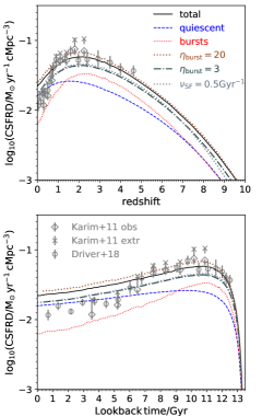
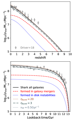
Figure 2: Cosmic SFR density (left panel) and stellar mass density (right panel) evolution for our default Shark model. Solid lines show all galaxies, while the dotted and dashed line show in the left panel show the contribution from the SBs and quiescent modes of star formation, and the dotted and dashed line in the right panel show the contribution of all stars formed during SBs driven by galaxy mergers and disk instabilities, respectively. The latter can de driven by both disk instabilities and mergers. Observations from Karim et al. (2011) and Driver et al. (2018) are also shown. We show three model variants adopting a lower/higher SF efficiency in SBs ($\eta_{\rm burst}=3$ and $\eta_{\rm burst}=20$, respectively; see $\S$ 4.4.3) and in quiescent SF ($\nu_{\rm SF}=0.5\,\rm Gyr^{-1}$; see Eq. 7), as labelled.

We solve these equations numerically using the Runge-Kutta Cash-Karp with adaptive stepsizes of the C++ GSL library. The accuracy to which the equations are solved are a parameter the user inputs into Shark (see Table 2 for the default value and name of this variable in the code).

The Eqs. 53-62 are the same in both star formation modes, quiescent (i.e. star formation in disks) and SB modes. The only difference is that during SBs $\dot{M}_{\rm cool}\equiv 0$. Ideally we would like to solve for the quiescent and SB modes simultaneously, and Shark will be progressing towards that more realistic representation of how star formation, outflows and inflows take place in galaxies. However, in the implementation of v1.1, we first solve for quiescent star formation and then for SBs.

5 Basic Results and Performance

In this section we present some basic results of Shark, focusing on some traditional tests, such as the SMF, and overall growth of galaxy stellar mass and SFR, but also on the gas content of galaxies and the universe. We also show scaling relations that relate galaxies’ masses, sizes, and metallicities in different components. For this section, we use our default model (see values adopted in parenthesis in Tables 3-4) using as backbone the L210N1536 simulation (unless otherwise stated), but also show model variations to aid our discussion and to show the reader some key systematic uncertainties in the model. All the observations shown throughout this paper have been scaled to our adopted cosmology and IMF when necessary.

The primary constraints we use to tune the free parameters are the $z=0,\,1,\,2$ SMFs, the $z=0$ the black hole-bulge mass relation and the mass-size relations. These are observations that we tried to fit as best as we could, although based on a visual inspection approach. Any other observables shown here are therefore “predictions” of the model (i.e. results that we did not fit for).

5.1 Baryon budget and its evolution

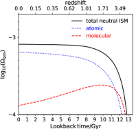
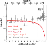
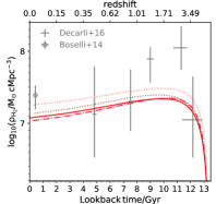
Figure 3: Left panel: Evolution of $\Omega_{\rm gas}\equiv\rho_{\rm gas}/\rho_{\rm crit}$, with $\rho_{\rm gas}$ and $\rho_{\rm crit}$ being the gas and critical densities, respectively. We show this for the total neutral gas in the ISM, HI and H₂, as labelled in our default Shark model. Middle panel: Evolution of $\Omega_{\rm HI}$ compared to the observational compilation of Rhee et al. (2018). The vertical dotted lines denotes the approximate redshift at which the hydrodynamical simulations of van de Voort et al. (2012) predict the transition from the HI being dominated by the ISM to the CGM of galaxies takes place. This transition is relevant as the Shark line here includes only HI in the ISM while the observations are not biased to detect ISM. We also show the two model variations shown in Fig. 2. Right panel: Evolution of $\rho_{\rm H2}$ compared to observations of Boselli et al. (2014) and Decarli et al. (2016). In this case we show density rather than $\Omega$ as it is the most common way observers express the density of H₂. We also show in the middle and right panels the same model variants as in Fig. 2.

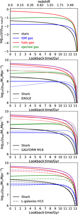
Figure 4: Top panel: The evolution of the contribution of several baryon reservoirs (see label) to the total baryon content of the universe locked up in halos (or that was at some point in halos) in our default Shark model. Second to bottom panels: Comparison of the density evolution of the baryon components in Shark with those of the EAGLE hydrodynamical simulations as analysed by Mitchell et al. (2018) (second panel), the GALFORM model in the variant of Mitchell et al. (2018) (third panel) and the L-galaxies model in the variant of Henriques et al. (2015) (bottom panel). Here, we also show the total baryon budget (the sum of the components shown) as magenta lines.

Fig. 2 show the evolution of the cosmic SFR and stellar mass densities, both in linear redshift (top) and lookback time (bottom). The former is useful to see in more detail how the model performs at high redshift, while the opposite is true for the latter. We compare with the observations of Karim et al. (2011), who used radio continuum detections and stacking, and from Driver et al. (2018), who presented a combined analysis of the surveys GAMA, G23-COSMOS and 3D-HST.

Regarding the cosmic SFR density, Shark agrees nicely with the observations at $z\gtrsim 1$, while producing slightly too much SFR at $z\lesssim 1$ by up to $\approx 0.15$ dex. We split the contribution from star formation in disks and SBs (blue and red lines, respectively) and find that overall disks dominate the cosmic SFR at $z\lesssim 1.7$ and $z\gtrsim 7$, with SBs making a significant contribution at $1.7\lesssim z\lesssim 5$ and becoming negligible at lower redshifts. Thus, the reason for the overproduction of stars at $z\lesssim 1$ is due to SF in disks. In principle we could increase the strength of AGN feedback to suppress SF in disks by suppressing cooling flows. However, we find that there is a tension at $z<1$ with the high mass end of the SMF (Fig. 5), such that a more effective AGN feedback would move the massive end towards lower masses, undershooting the observational SMF. Interestingly, Shark reproduces quite well the stellar mass density evolution (right panels in Fig. 2), with some minor tension arising at $z\gtrsim 4$. This shows that the tension seen in the cosmic SFR vanishes when looking at the stellar mass density. There has been a long standing tension between these two measurements (see discussion in Driver et al. 2018) and thus, we decide to not tune for the cosmic SFR.

The right panels of Fig. 2 show the contribution to the stellar mass density from SBs triggered by galaxy mergers and disk instabilities. Galaxy mergers are the main driver of stellar mass growth due to SBs. Disk instabilities start contributing more significantly at $z\lesssim 1$ and by $z=0$ they contribute about $35$% of the total stellar mass ever formed in SBs. We find that the contribution from SBs have an important effect on the overall cosmic SFR density. As an example of that, we show in Fig. 2 the predictions of a model in which the SF law for SBs is assumed to have a lower/higher normalization relative to SF in disks ($\eta_{\rm burst}=3$ and $\eta_{\rm burst}=20$; see $\S$ 4.4.3). We find that decreasing $\eta_{\rm burst}$, decreases the cosmic SFR density throughout time by $\approx 0.1-0.15$ dex, but increasing it has less of an effect. In Shark, we find that the effect of $\eta_{\rm burst}$ saturates at values $\gtrsim 7$, which is due to the gas depletion timescale being always comfortably shorter than the Hubble time in those cases. This is no longer true when $\eta_{\rm burst}\lesssim 7$ and when the SF efficiency is considerably lower than the $1\,\rm Gyr^{-1}$ adopted in our default model. The latter can be seen from the variation with $nu_{\rm SF}=0.5\,\rm Gyr^{-1}$ in Fig. 2. A higher $\eta_{\rm burst}$ in the case of $nu_{\rm SF}=0.5\,\rm Gyr^{-1}$, allows us to recover the same overall cosmic SFR density evolution as our default model.

Fig. 3 shows the evolution of the total ISM mass in galaxies, and the contributions from atomic and molecular gas (left panel) in our default Shark model. Molecular gas dominates the ISM budget of galaxies at $z\gtrsim 2.5$, while HI dominates at lower redshifts. The H₂ density peaks at $z\approx 1.7$, which is lower than the peak of the cosmic SFR density ($z\approx 2$). This is due to the different effect SBs have on the cosmic SFR and H₂ densities. SBs contribute significantly to the SFR density, helping to shift the SFR density peak to higher redshifts, while their contribution to the H₂ density is minor. The latter is due to the short H₂ depletion times adopted for SBs. This is similar to what was seen in the Eagle hydrodynamical simulations (Lagos et al., 2015). The offset between the peaks of the cosmic SFR and $\Omega_{\rm mol}$ is exacerbated for larger values of $\eta_{\rm burst}$ (the parameter controlling the normalisation of the SF law of bursts relative to star formation in disks; see $\S$ 4.4.3), while becoming smaller if $\eta_{burst}\rightarrow 1$. This is seen as a shift in the cosmic SFR density peak in that model (see dot-dashed line in Fig. 2).

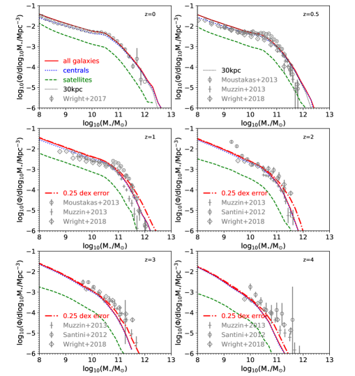
Figure 5: Galaxy SMF at $z=0$, $z=0.5$, $z=1$, $z=2$, $z=3$ and $z=4$, as labelled, for our default Shark model. Solid lines show all galaxies, while dotted and dashed lines show central and satellite galaxies, respectively. We also show observations from Wright et al. (2017), Wright et al. (submitted), Muzzin et al. (2013), Moustakas et al. (2013), Santini et al. (2012), as labelled. For reference, the dot-dashed line in the middle and bottom panels show the SMF if we assume stellar masses have a Gaussian uncertainty of width $0.25$ dex. We also show at $z=0$ and $z=0.5$ the SMF if we use the mass enclosed in a $30$ physical kpc aperture rather than the total stellar mass (black dotted line in the top panels).

The middle and right panels of Fig. 3 compare our predicted HI and H₂ densities (only hydrogen; i.e. removing the contribution from Helium) with the observations of Boselli et al. (2014) and Decarli et al. (2016), in the case of H₂, and Rhee et al. (2018), for HI. We see that Shark reproduces the HI observations at $z\lesssim 1.5$ very well, while deviating significantly at higher redshifts. The latter is not necessarily a failure of the model, as here we only show HI in the ISM of galaxies, while observations are not biased to detecting ISM gas. van de Voort et al. (2012), using cosmological hydrodynamical simulations of galaxy formation, showed that at $z\gtrsim 2$ the neutral gas abundance of the universe from $z=3.5$ to $z=0$, is expected to be dominated by circumgalactic gas rather than the ISM of galaxies. Since Shark does not account for the fraction of HI in the halo gas, we do not necessarily expect to be able to reproduce the observations at $z\gtrsim 1.5$. The model variants adopting a different efficiency in SF in disks or SBs has little effect on the HI density evolution despite having an effect on the evolution of the cosmic SFR and H₂ densities (see discussion below).

In the case of H₂, we find that Shark predicts an H₂ density that agrees well with observations, except at the peak, where our model produces too little H₂ abundance. The peak of the H₂ evolution is very sensitive to how star formation is modelled in Shark. In the model variant in which SBs are less efficient ($\eta_{\rm burst}\approx 3$) than in our default model, the H₂ density peak is $\approx 0.08$ dex lower than in our default Shark model, while increasing $\eta_{\rm burst}$ has little effect. Adopting $\nu_{\rm SF}=0.5\,\rm Gyr^{-1}$ has a much more important effect on the H₂ density evolution, increasing it by $\approx 0.2$ dex.

Fig. 4 shows the breakdown of the $4$ key baryon components in Shark, the total stellar mass, ISM mass, halo gas (gas inside the halos and outside galaxies) and ejected gas (gas outside halos). Note that these baryons are those currently, or that were in the past, in halos. The fraction of baryons outside halos can be as large as $\approx 60$% according to observations (Shull et al., 2012; Driver et al., 2018), while the fraction of DM that is unbound to halos with masses $\gtrsim 10^{10}\,\rm M_{\odot}$ can be up to $50$% (Shattow & Croton, 2015), accounting for most of that gas (if we assume the universal baryon fraction).

In Shark, the total baryon budget of galaxies is dominated by ISM gas at lookback times $\gtrsim 9$ Gyr ($z\approx 1.3$), while stellar mass becomes dominant at later times. However, galaxies never dominate the baryon content of the universe. Halo gas is overall the most dominant baryon component, with the ejected halo gas contributing similarly to the halo gas at lookback times $\gtrsim 12$ ($z\gtrsim 3.5$). The latter is due to the high specific star formation rates of high redshift galaxies and the redshift dependence of the outflow rate. The latter translates into more powerful outflows at high redshift (as $\rm z_{\rm P}>0$ in Eq. 33). The latter is adopted following the FIRE results of Muratov et al. (2015).

Mitchell et al. (2018) studied the growth of the same baryon components of Fig. 4 for the GALFORM semi-analytic model and the EAGLE hydrodynamical simulations. In the second to fourth panels of Fig. 4 we compare Shark with EAGLE, GALFORM and the L-galaxies SAMs, respectively. Shark behaves similarly to L-galaxies in the sense that halo gas always dominate the baryon budget. GALFORM has the ejected gas component dominating at early times (lookback time $\gtrsim 9.5$), but the halo gas dominates over most of the history of the universe. EAGLE displays a different behavior to Shark, GALFORM and L-galaxies as the majority of baryons throughout the history of the universe are locked up in the ‘ejected’ component, except at lookback times $<4.5$ Gyr where the halo gas starts to dominate. Note that Mitchell et al. (2018) calculated this ejected mass as the difference between the baryons accounted for inside the halos and the universal baryon fraction, thus it is not strictly the same as the ejected component in SAMs. The comparison is, however, a fair one, as all the SAMs by construction have a total baryon fraction (including the ejected component) per halo equal or close to the universal baryon fraction. Thus, the most striking difference here is that overall EAGLE has much less baryons inside halos than the three SAMs. This can happen either because the gas accretion onto halos is less efficient than the DM accretion or because feedback is very effective at ejecting gas from halos. In the former case, feedback can still play a key role as outflows can interact with the gas that is outside halos, preventing it from ever inflowing onto halos. Note that the overall efficiency of outflowing gas in Shark, GALFORM and EAGLE are similar at lookback times $\lesssim 9$ Gyr and $>7$ Gyr, respectively, as the ejected gas baryon component is similar between the models (green lines in the second and third panels of Fig. 4), while the L-galaxies one is lower by a factor of $\approx 2.5-3$ compared to Shark and GALFORM, and $\approx 4$ compared to EAGLE. Another important effect is the exact definition of halo mass, as the amount of baryons scales with it. Different definitions, FOF mass, $M_{\rm crit,200}$, $M_{\rm mean,200}$, etc., can differ by factors of up to a few (Jiang et al., 2014). The Shark DM mass function agrees very well with the mean $200$ density mass function of Sheth et al. (2001), produced using the Planck Collaboration et al. (2016) cosmology and HMF calc (Murray et al., 2013). These masses, however, are generally larger than the Dhalo masses used in GALFORM and the subfind masses of EAGLE and L-galaxies. The latter leads to the total baryon density of Shark being slightly larger than the other models (dark magenta lines in Fig. 4).

In summary, the main difference between the SAMs and EAGLE is that in the latter the amount of baryons inside halos is much smaller. This is an important physical effect that is currently not included in any SAM to our knowledge, but could relax significantly the AGN feedback efficiency required in SAMs to prevent the large amounts of halo gas from cooling and forming stars. This is because in EAGLE, the baryon fractions inside halos is less than the universal one even for massive halos ($M_{\rm halos}\sim 10^{14}\rm\,M_{\odot}$; see Fig. $8$ in Mitchell et al. 2018), with deviations being larger at increasing redshift; while in SAMs, the baryon fraction inside halos becomes significantly lower than the universal one only at $M_{\rm halo}\lesssim 10^{11.5}\rm\,M_{\odot}$. Remarkably, the stellar mass density evolution of Shark and EAGLE are within $15$% of each other, while with GALFORM and L-galaxies differences increase to up to $40$% and $25$%, respectively. This is crucial evidence showing that effectively the same stellar mass density can be obtained for very different physical reasons.

5.2 Stellar masses and their scaling with halo mass

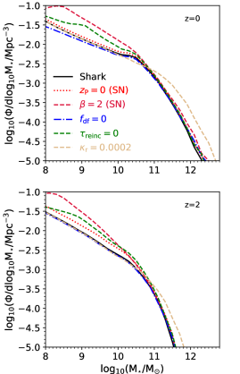
Figure 6: Galaxy SMF at $z=0$ and $z=2$, as labelled, for our default Shark model and 5 variations perturbing the stellar feedback parameter (red lines), dynamical friction timescale (blue line), reincorporation timescale of the ejected gas (green line) and the AGN feedback efficiency (tan line). See text for details.

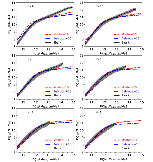
Figure 7: Stellar mass as a function of halo mass for centrals galaxies in our default Shark model at $z=0$, $z=0.5$, $z=1$, $z=2$, $z=3$ and $z=4$, as labelled. Solid lines with shaded regions show the median and the $16^{\rm th}-84^{\rm th}$ percentile ranges. Here, we show all bins with $\geq 10$ objects. We also show the empiral results of Moster et al. (2013) and Behroozi et al. (2013a).

SMFs and the stellar-halo mass relation have become a key test for models and are now the usual observational choice for the tuning of free parameters in semi-analytic models (Guo et al., 2011; Henriques et al., 2013; Knebe et al., 2017; Cora et al., 2018) and hydrodynamical simulations (Schaye et al., 2015; Wang et al., 2015; Pillepich et al., 2018). We therefore also study these relations to understand the behaviour of Shark.

Fig. 5 shows the SMF of Shark at several redshifts, from $z=0$ to $z=4$. This is shown for the entire galaxy population and for centrals and satellites separately. Here, satellites include galaxies in satellite subhalos and orphan galaxies, as described in $\S$ 4.1. We also show a compilation of observations covering the same redshift range. We are able to reproduce very well the SMF up to $z=3$, while at higher redshifts the model struggles to reproduce the high-mass end, even in the case a small Gaussian uncertainty of $0.25$ dex is included. The latter is a typical error at high redshift (Marchesini et al., 2009; Mitchell et al., 2013), and is enough to alleviate the small tension at the massive end at $z=2$ and $z=3$. At the high-mass end and at $z<1$, Shark produces slightly more mass than observed at fixed number density. This may not be very well converged at the resolution of the L210N1536, as our higher resolution SURFS run L40N512 produces slightly less massive galaxies at fixed number density, in better agreement with the observations (see discussion in Appendix A). In addition, (see discussion in Bernardi et al. 2013) the exact high-mass end of the SMF is a fairly contested topic in observations, as the exact contribution from the intra-cluster light is uncertain. This is why several cosmological hydrodynamical simulations tend to show the stellar mass contained in an spherical aperture (Schaye et al., 2015; Pillepich et al., 2018). We show the effect of using a fixed aperture of $30$ physical kpc in the SMF at $z=0$ and $z=0.5$. We calculate the stellar mass enclosed by assuming an exponential and a Plummer profiles for the stellar disk and bulge, respectively, with half-stellar mass radii calculated as in $\S$ 4.4.12 (see $\S$ 5.4 for a comparison with observations). The number density at the very high-mass end decreases, albeit only a small amount. Fig. 5 also shows that central galaxies always dominate at the high-mass end, while satellite galaxies have a negligible contribution at high redshift, but become increasingly important towards low redshift at the low-mass end.

The normalization and flatness of the SMF at the low-mass end throughout redshift has been challenging to reproduce in semi-analytic models (Henriques et al., 2013), but as Fig. 5 shows, Shark does not struggle with this. This is the result of a combination of effects: dynamical friction modelling, mass loading of the stellar feedback model depending very strongly on $V_{\rm circ}$, a slow reincorporation timescale and the weak redshift dependence of the stellar feedback efficiency. At the massive end, the main physical process controlling the steep decline in number density is AGN feedback in high mass halos. This is shown in Fig. 6, in which we show model variations adopting a dynamical friction efficiency $f_{\rm df}=0$ (i.e. satellites merge onto the central as soon as they become orphans; blue dotted line), a weaker scaling of the mass loading on $V_{\rm circ}$ ($\beta=2$; see Eqs. 29-32; red, dashed line), removing the redshift dependence of the stellar feedback efficiency ($\rm z_{\rm P}=0$; see Eqs. 31 and 33; red, dotted line), assuming instantaneous reincorporation of the ejected gas ($\tau_{\rm reinc}=0$; see Eq. 34; green, dashed line), and adopting an AGN feedback efficiency $10$ times lower ($\kappa_{\rm r}=0.0002$; see Eq. 44; tan, dashed line).

Merging galaxies instantaneously after they become orphans ($f_{\rm df}=0$) has the effect of producing a flatter low-mass end of the SMF and an overall lower abundance of galaxies below the knee, which is more clearly seen at $z=0$. In the case of stellar feedback, removing the redshift dependence of the mass loading ($\rm z_{\rm P}=0$) has little effect by $z=0$, but at $z=2$ the model produces a higher abundance of galaxies below the knee of the SMF, in tension with the observations. A weaker scaling of the mass loading on $V_{\rm circ}$ ($\beta=2$) has a dramatic effect on the abundance of low mass galaxies at both redshifts, though not affecting the high-mass end. This shows that a strong dependence on $V_{\rm circ}$ is required in order to reproduce the flat low-mass end. Finally, the reincorporation timescale has also a clear effect on the low-mass end, which is more obvious at $z=2$. Henriques et al. (2013) suggested that long reincorporation timescales are required to fit the low-mass end of the SMF at high redshift. Although this is seen in Shark, it is important to stress that this is not a unique solution, as Fig. 6 shows the complex dependence that the low-mass end of the SMF has on several, different physical processes. At the massive end, reducing the AGN feedback efficiency by a factor of $10$ produces a shallower decrease in the number density beyond the knee of the SMF. The effect is, however, non-linear as the number density of galaxies with $M_{\rm star}\approx 10^{12}\,\rm M_{\odot}$ increases by only $\approx 2$.

Although our primary constraint to tune the free parameters is the SMF, we did not use the stellar-halo mass relation in that process. Thus, we can use it to study whether Shark places the right amount of stellar mass in different halo masses. This is an important test as it can be viewed as a halo star formation efficiency. Fig 7 shows the stellar-halo mass relation at several redshifts from $z=0$ to $z=4$, compared to the empirical estimates of Moster et al. (2013) and Behroozi et al. (2013a). The agreement between Shark and Behroozi et al. (2013a) is good over the entire redshift range at halo masses $\lesssim 10^{13}\,\rm M_{\odot}$, while at $z=0$ we find that the stellar mass is lower at fixed halo mass compared to Moster et al. (2013). The differences between Moster et al. (2013) and Behroozi et al. (2013a) can be considered part of the systematic uncertainties of the measurement. At high halo masses, $M_{\rm halo}\gtrsim 10^{13}\,\rm M_{\odot}$, we find that Shark has a slow that is slightly too steep compared to Moster et al. (2013) and Behroozi et al. (2013a), which means that by $M_{\rm halo}\approx 10^{15}\,\rm M_{\odot}$, central galaxies in Shark are $\approx 1.4-8.5$ (i.e. the $16^{\rm th}-84^{\rm th}$ percentile range) times too massive compared to Moster et al. (2013). This is not entirely surprising, as both the Moster et al. (2013) and Behroozi et al. (2013a) empirical stellar-halo mass relations were calibrated using the stellar mass function of Li & White (2009), which has a high-mass end that is steeper than the Wright et al. (2017) stellar mass function. The latter is the one we use as calibration reference.

Guo et al. (2016) presented a comparison between EAGLE (Schaye et al., 2015) and two widely known semi-analytic models L-galaxies (Guo et al., 2011) and GALFORM (Gonzalez-Perez et al., 2014). One of the key comparisons was the stellar-halo mass relation and they found that the three models agreed relatively well but they displayed very different scatter, with EAGLE having the tightest relation ($\approx 0.4$ dex). An interesting feature of Shark and that is evident in Fig 7 is that it predicts a very tight relation with a $1\sigma$ scatter of $\approx 0.35-0.5$ dex depending on the halo mass. This value is much smaller than the semi-analytic models L-galaxies and GALFORM, and similar to EAGLE, though still larger than the empirical estimates of Moster et al. (2013) and Behroozi et al. (2013a). Mitchell et al. (2016) showed that adopting a scaling with the halo velocity, as adopted in Shark, or the galaxy velocity for stellar feedback has an important effect on the scatter. In the future we will investigate the effect different physical processes have on the scatter of this relation in Shark.

5.3 Gas mass functions and scaling relations

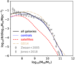
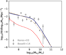
Figure 8: Atomic (top) and molecular (bottom) hydrogen MFs at $z=0$, for our default Shark model. Solid lines show all galaxies, while dotted and dashed lines show central and satellite galaxies, respectively. We show observations of the HI MF from Zwaan et al. (2005) and Jones et al. (2018), and from Keres et al. (2003) and Boselli et al. (2014) for the H₂ MF. We also show as dot-dashed line a variant of the model adopting the GD14 star formation law (rather than the BR06; see $\S$ 4.4.2).

Lagos et al. (2011b, a) showed that the HI and H₂ mass functions (MFs) and their scaling with stellar mass are a key test to the star formation modelling in simulations. The stellar mass and SFR of galaxies are only mildly affected by the modelling of star formation, because inflows and outflows tend to quickly self-regulate and erase the effect a higher/lower efficiency star formation model could have. However, the gas properties of galaxies are very sensitive to this choice. We did not use these MFs in the process of parameter tuning, and thus comparing the HI and H₂ abundance of galaxies with observations represents a test of how well the model does.

Fig. 8 shows the $z=0$ HI and H₂ MFs of our default Shark model. We show all the galaxies, and the contribution from centrals and satellites. We show the observed HI MF of Zwaan et al. (2005) and Jones et al. (2018), which were obtained using the HI Parkes All-Sky Survey (HIPASS; Meyer et al. 2004) and the Arecibo Legacy Fast ALFA Survey (ALFALFA; Haynes et al. 2018), respectively. In the case of the H₂ MF, we show the inferences of Keres et al. (2003) and Boselli et al. (2014). These observations correspond to CO$\rm(1-0)$, which we convert to H₂ by adopting a Milky-Way like $\rm CO(1-0)$-H₂ conversion factor (Bolatto et al., 2013), $N_{\rm H_{2}}/\rm cm^{-2}=2\times 10^{-20}\,I_{\rm CO}/\rm K\,km\,s^{-1}$. Note that these observations provide an indirect measurement of the MF as they are not blind surveys, but correspond to the follow-up galaxy samples selected from their $60\,\rm\mu m$ in the case of Keres et al. (2003) and from the Herschel Reference Survey in the case of Boselli et al. (2014).

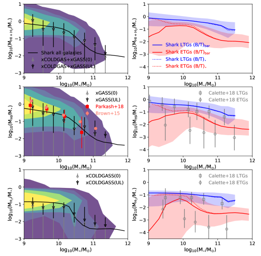
Figure 9: Gas scaling relations at $z=0$ for our default Shark model: total neutral gas (atomic plus molecular; top panels), HI (middle panels) and molecular gas (bottom panels) fractions as a function of stellar mass. Left panels show all the galaxies, while the right panels show the population split into ETGs and LTGs, as labelled. We show two definitions of ETGs/LTGs, one based on the stellar plus gas mass fraction contributed by the bulge, $(\rm B/T)_{\rm bar}$, and another one based on stellar mass alone, $(\rm B/T)_{\star}$. Ratios $\geq 0.5$ and $<0.5$ are considered ETGs and LTGs, respectively. Lines show the median of the populations, while the contours in the left panel show percentile ranges from $99^{\rm th}$ to $10^{\rm th}$, and the shaded regions on the right panels show the $16^{\rm th}-84^{\rm th}$ percentile ranges. The latter are shown only for the $(\rm B/T)_{\rm bar}$ classification, for clarity. Medians are shown for all bins with $\geq 10$ objects. Symbols with errorbars show the median and the $1\sigma$ scatter of the observations of xGASS (Catinella et al., 2018), the stellar mass-selected sample of Parkash et al. (2018), HI stacking of Brown et al. (2015) and xCOLDGASS (Saintonge et al., 2017) (left panels), and the observationally derived gas fraction scaling relations for early- and late-type galaxies from Calette et al. (2018) (right panels). Downwards triangles show the observations if non-detections are set to their upper limit (referred to as ‘UL’), while upward triangles show the results of non-detections are set to zero (referred to as ‘0’).

Shark predicts an HI MF in reasonable agreement with the observations, except for the slight overproduction of galaxies with $M_{\rm HI}\gtrsim 10^{11}\,\rm M_{\odot}$. This may not be entirely surprising as for Shark we show the total HI mass in the ISM of galaxies, while observations are subject to some level of HI self-absorption which may lie at the $10-20$% level (going up to $40$% in dense regions; Braun et al. 2009). The decrease in number density at $M_{\rm HI}\lesssim 10^{8}\,\rm M_{\odot}$ is due to a combination of the resolution of the L210N1536 simulation, which does not allow us to have a complete sample of the halos that would host these galaxies, $M_{\rm halo}\lesssim 10^{10}\,\rm M_{\odot}$, and the photo-ionisation modelling (see convergence tests in Appendix A). As expected, the HI MF is dominated over the entire mass range by central galaxies, with satellites becoming important only at $M_{\rm HI}\lesssim 10^{8}\,\rm M_{\odot}$. The latter is due to the environmental effects included in Shark, which assume instantaneous stripping of the halo gas of galaxies as soon as they become satellites and photo-ionisation feedback affecting low-mass central galaxies. In the absence of gas accretion, satellites can quickly use up their gas by continuing star formation and the driving of outflows. The presence of outflows means that the ISM gas consumption can happen faster than the instantaneous ISM depletion timescale. For low-mass centrals, the Sobacchi & Mesinger (2013) model applied in Shark, prevents gas cooling from taking place in these galaxies and thus the HI is not replenish.

The H₂ MF of Shark is also in reasonable agreement with the observational inferences shown in the bottom panel of Fig. 8. We do, however, warn that the systematic uncertainties, mostly due to the $\rm CO(1-0)$-H₂ conversion factor, and the fact that we lack a CO blind survey, are large (Obreschkow et al., 2009). An interesting feature is that the low-mass end of the H₂ MF in Shark is flatter than the HI MF. This means that low HI mass galaxies have a larger contribution to the cosmic HI density that the contribution of their low H₂ mass counterparts to the cosmic H₂ density. We also show in Fig. 8 a variation of our default Shark model, adopting the GD14 rather than the BR06 star formation law (see $\S$ 4.4.2 for details). Interestingly, the H₂ MF is only slightly affected by this choice, while the HI MF changes dramatically at $M_{\rm HI}\lesssim 10^{10.2}\rm\,M_{\odot}$. This is due to galaxy self-regulation, in which the dense gas mass adapts to give the same SFR and stellar mass growth, while the HI is in principle free to change regardless of self-regulation (see discussion in Lagos et al. 2014a). This is a good example of the effect of self-regulation on the galaxy’s ISM content.

The left panels of Fig. 9 show the neutral hydrogen (HI plus H₂), HI and H₂ gas to stellar mass ratios as a function of stellar mass at $z=0$ for our default Shark model. We compare with the observations of Saintonge et al. (2017), for H₂, and Brown et al. (2015), Parkash et al. (2018) and Catinella et al. (2018), for HI. Catinella et al. (2018) and Parkash et al. (2018) studied individual galaxies with $M_{\star}>10^{9}\,\rm M_{\odot}$, and thus are better suited at measuring the scatter of the gas fraction scaling relations than Brown et al. (2015), who performed HI spectral stacking. In the latter, a higher gas fraction is expected, as it is effectively a mean HI-to-stellar mass ratio in real space rather than the median on the logarithmic space. We find that Shark predicts gas fractions in reasonable agreement with the observations. Shark may be producing slightly too much neutral gas at fixed stellar mass, but still comfortably within the scatter and uncertainties in the observations. In the future we will compare the HI-to-stellar mass ratio distributions in different stellar mass bins, as this may be able to offer new constraints to models (Lemonias et al., 2013).

In the right panels of Fig. 9 we show the same gas scaling relations but separating late- (LTGs) and early-type (ETGs) galaxies. We define these in two ways, based on the bulge-to-total stellar plus gas mass ratio, $(\rm B/T)_{\rm bar}$, and on the bulge-to-total stellar mass ratio, $(\rm B/T)_{\star}$, where ratios above (below) $0.5$ correspond to ETGs (LTGs). LTGs are characterised by much higher gas fractions at fixed stellar mass than ETGs, with those differences being larger for H₂ than for HI. The latter is due to the star formation law assumed for star formation in bulges being dependent on the surface density of the gas. As the latter decreases, the conversion of HI into H₂ becomes less efficient (due to lower pressure), and thus less stars are formed, depleting the HI gas in longer timescales. Thus, HI can be preserved for longer compared to H₂. We also show observational inferences of Calette et al. (2018) for the gas fractions for LTGs and ETGs, who analysed in a self-consistent way a large compilation of HI and H₂ observations in the local Universe. We find that the observations suggest that the difference between LTGs and ETGs is larger than that obtained in Sharkat $M_{\star}\gtrsim 10^{10}\rm\,M_{\odot}$, regardless of the way we select ETGs/LTGs in the model, which may be connected with the fact that we do not yet include in Shark environmental processes that strip the ISM of galaxies. Those will be included in future versions of Shark, and this issue will be explored in detail. At $M_{\star}\lesssim 10^{10}\rm\,M_{\odot}$, we see a reversal of the relation in the case of the $(\rm B/T)_{\rm bar}$, due to the effect of gas-rich disks being assigned to the LTG population. Those are classify at ETGs if we instead use the $(\rm B/T)_{\star}$, as their stellar mass is dominated by the bulge, but their baryon mass (gas plus stars) is dominated by the disk, due to the presence of very gas-rich disks.

5.4 Galaxy sizes and morphology

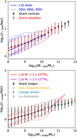
Figure 10: Size-stellar mass relation for disks (top panel) and bulges (bottom panel) at $z=0$. Note that here we plot disk (bulge) half-stellar mass radii vs. disk (bulge) stellar mass. Here, we show all bins with $\geq 10$ objects. The top panel shows only LTGs in Shark ($\rm(B/T)_{\star}<0.5$), separating into centrals and satellites. The bottom panel shows Shark ETGs ($\rm(B/T)_{\star}\geq 0.5$). Symbols with errorbars show the medians and $16^{\rm th}-84^{\rm th}$ percentile ranges, respectively. In the bottom panel we also show the relation for bulges with stellar masses $>10^{10}\,\rm M_{\odot}$ that mostly grew by galaxy mergers (diamonds) or by disk instabilities (squares). We also show a model variant that assumes no gas dissipation during mergers (see Eq. 51; crosses). Solid and dotted lines show the best fit and the $50^{\rm th}$, $68^{\rm th}$ and $90^{\rm th}$ percentile regions of the GAMA observations of Lange et al. (2016).

Fig. 10 shows the disk size-disk mass relation, and the equivalent for bulges. We compare with the observations of Lange et al. (2016), who performed profile light fitting to decompose their galaxies into disks and bulges. They then measured the sizes and the stellar masses of both components. Galaxy disks agree very nicely with the observations of Lange et al. (2016). Central galaxies in Shark tend to have more extended disks than satellites, due to the latter forming at earlier times, where DM halos had lower specific angular momentum. The region with $M_{\rm disk}\gtrsim 10^{11}\,\rm M_{\odot}$ is scarcely populated in observations. This is also the case in Shark  as we find that of the $764,135$ galaxies with $M_{\rm disk}>10^{8}\,\rm M_{\odot}$ that have $\rm(B/T)_{\star}<0.5$, only $50$ have $M_{\rm disk}>10^{11}\,\rm M_{\odot}$.

Shark bulges have sizes that are good agreement with the observations, though they tend to be slightly too large at around bulge masses of $10^{10}\,\rm M_{\odot}$. We find that this is mostly due to the effect of galaxy mergers. This can be seen from the squares and diamonds in the lower panel of Fig. 10, which show the sizes of bulges with stellar masses $>10^{10}\,\rm M_{\odot}$ that grew mostly due to disk instabilities and galaxy mergers, respectively. We only show massive bulges in these two cases as at lower masses bulges mostly form and grow due to galaxy mergers. Bulges formed via disk instabilities tend to be $\approx 0.15$ dex larger than those produced by galaxy mergers around a bulge mass of $10^{11}\,\rm M_{\odot}$. The latter is mostly due to the effect of gas dissipation during mergers that is included in our default Shark model becoming negligible around that stellar mass (see description in $\S$ 4.4.7). If we do not include the effects of dissipation, bulges become unrealistically large (see crosses in Fig. 10) below a bulge mass of $10^{10}\,\rm M_{\odot}$. Both mass ends are affected by gas-rich mergers, at later (early) times in the case of the low-(high-)mass end. Thus, we find that dissipation is a key process that has to be considered in order to reproduce realistic bulge sizes. This agrees with the conclusion of Zoldan et al. (2018) using the GAEA SAM. Reproducing the bulge sizes of galaxies has been a long standing challenge for SAMs (e.g. Lacey et al. 2016; Zoldan et al. 2018), and thus we consider the agreement with the bulge sizes obtained by Shark an important success.

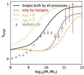
Figure 11: The total fraction of stellar mass contributed by bulges as a function of stellar mass at $z=0$ in our default Shark model. Symbols with errorbars show the median and $1\sigma$ uncertainty in the observations of Moffett et al. (2016). We also show two model variants changing the threshold $\epsilon_{\rm disk}$ below which galaxies are considered unstable (see Eq. 4.4.8), as labelled.

Another important test for galaxy formation models, is whether they place the right amount of stellar mass into disks and bulges. Moffett et al. (2016) measured the SMF separating galaxies into different morphological types and also into disks/bulges. With this, they derived the fractional contribution from bulges/disks to the total stellar mass in bins of stellar mass. This is quite a difficult measurement to do in observations as light profile fitting is required, which can be robustly done in very disk- and bulge-dominated galaxies, but when both components contribute similarly, the measurement is less robust (Robotham et al., 2017). In Fig. 11, we compare Shark with these measurements for two measurements of bulge mass. The first one is considering all the mass in the central concentration (regardless of whether it was formed due to mergers or disk instabilities; solid line), and the second one assumes that the bulge mass formed through disk instabilities (either through the starburst triggered by the gas being fueled to the centre or the stars that are transferred from the disk to the bulge) is part of the disk (dashed line). The bulge mass formed via mergers include both the stars formed via merger-driven starbursts and stars that were accreted by the bulge as a result of a merger (but that were formed in the disk of the primary and/or in the secondary galaxies). The latter is done as pseudobulges in Moffett et al. (2016) were added up to the disk rather than the bulge, and those are thought to form through secular processes taking place in the disks of galaxies (Kormendy & Kennicutt, 2004). The effect of assigning the bulge mass formed via disk instabilities to the disk has the effect of shifting the transition from disk- to bulge-dominated stellar budget to higher stellar masses, much closer to the Moffett et al. (2016) observations. In Shark, we find that the formation of elliptical galaxies (i.e. spheroid dominated, massive galaxies) is dominated by galaxy mergers rather than disk instabilities, as disk instabilities only increase the bulge contribution by $\approx 10$% at $10^{11}\,\rm M_{\odot}$. This is qualitatively similar to the finding in large cosmological hydrodynamical simulations that elliptical galaxies form primarily via galaxy mergers (Wellons et al., 2016; Clauwens et al., 2018; Lagos et al., 2018a).

The transition from disk- to bulge-dominated stellar budget is very sensitive to the value of the threshold $\epsilon_{\rm disk}$ below which galaxies are considered unstable (see Eq. 4.4.8). This is seen in the model variants shown in Fig. 11, adopting $\epsilon_{\rm disk}=0$ (dot-dashed line) and $\epsilon_{\rm disk}=1$ (dotted line). When no disk instabilities take place, the transition to bulge-dominated stellar budget moves by $\approx 0.5$ dex to higher stellar masses, while adopting a much larger $\epsilon_{\rm disk}$ moves the transition by $\approx-0.5$ dex. We find that values of $\epsilon_{\rm disk}\lesssim 0.4$, lead to the bulge growth to be dominated by galaxy mergers, while the opposite is true for larger values of $\epsilon_{\rm disk}$. We find that in Shark $f_{\rm bulge}$ tends to $0.15$ as stellar mass decreases. This is due to gas-rich mergers taking place in dwarf galaxies. We find that centrals tend to have a lower incidence of bulge-dominated galaxies than satellites at $M_{\star}\lesssim 10^{10.8}\,\rm M_{\odot}$, at which point the trend reverses (not shown here).

5.5 The BH population

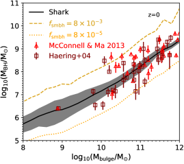
Figure 12: The BH-bulge mass relation at $z=0$. The solid line and shaded region correspond to the median and the $16^{\rm th}-84^{\rm th}$ percentile ranges for our default Shark model. Here, we show all bins with $\geq 10$ objects. Triangles with errorbars show the local observations of Häring & Rix (2004) and McConnell & Ma (2013), as labelled. We also show the medians of two model variations that change the efficiency of the gas inflow towards the SMBH during starbursts by $\times 10$ ($f_{\rm smbh}=8\times 10^{-3}$) and $:10$ ($f_{\rm smbh}=8\times 10^{-5}$), as labelled.

Like most SAMs and hydrodynamical simulations, Shark uses the BH-bulge mass relation to tune its free parameters (e.g. Schaye et al. 2015; Lacey et al. 2016). In Shark, this relation is pretty much controlled by a single parameter, and that is the efficiency at which gas flows towards the central BH during starbursts ($f_{\rm smbh}$ in Eq. 41). We show in Fig. 12 the BH-bulge mass relation at $z=0$ for our default Shark model, and two variants adopting a $f_{\rm smbh}$ $10$ times higher/lower than our optimal value. These changes almost linearly translate into the same change in the normalisation of the BH-bulge relation (see dashed and dotted lines in Fig. 12). We also show in Fig. 12 the observations of Häring & Rix (2004) and McConnell & Ma (2013), which were used as reference to obtain an optimal $f_{\rm smbh}$. In the future we will explore the QSO luminosity functions as they offer independent tests to assess how realistic the BH population in Shark is.

5.6 The Main sequence and mass-metallicity relation

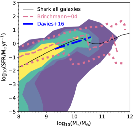
Figure 13: SFR vs. stellar mass at $z=0$ for our default Shark model. Here, we include all the galaxies that have an $\rm SFR/M_{\star}>10^{-3}\,\rm Gyr^{-1}$ and show the median only for bins with $\geq 10$ objects. Contours show percentiles ranges ranging from $99^{\rm th}$ to $10^{\rm th}$, from the outer to the inner regions. The dashed line shows the median of all galaxies. The dashed and thick dotted lines show the median and the region of $0.02$ conditional likelihood of SFR given a stellar mass from Brinchmann et al. (2004). The dot-dashed line shows the best fit of the GAMA main sequence reported by Davies et al. (2016).

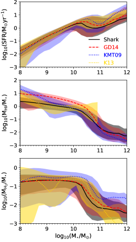
Figure 14: Top panel: main sequence in the SFR vs. stellar mass at $z=0$, calculated with all the galaxies that have an $\rm SFR/M_{\star}>10^{-3}\,\rm Gyr^{-1}$, for our default Shark model and 3 variants adopting the GD14, KMT09 and K13 star formation laws (see $\S$ 4.4.2 for details). Lines show the median while shaded regions show the $16^{\rm th}$ and $84^{\rm th}$ percentiles. Bottom panels: the HI- (middle) and H₂-to-stellar mass ratio (bottom) as a function of stellar mass at $z=0$ for the same models as in the top panels.

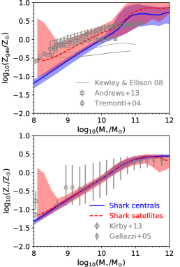
Figure 15: Top panel: Gas metallicity vs. stellar mass as $z=0$, for our default Shark model. Solid and dashed lines show the median of centrals and satellites, respectively. shaded regions show the $16^{\rm th}-84^{\rm th}$ percentile ranges. Here, we show all bins with $\geq 10$ objects. Symbols show the observations of Tremonti et al. (2004) and Andrews & Martini (2013), as labelled, while lines show $4$ measurements of Kewley & Ellison (2008), which were produced using different methods to derive metallicities. The $4$ relations correspond to those giving the lowest/highest normalisation and provide a measurement of the systematic uncertainty. Bottom panel: As in the top panel but for the stellar metallicity. Here we show observational inferences from Gallazzi et al. (2005) and Kirby et al. (2013), as labelled.

The self-regulation of galaxies, i.e. the idea of SF regulating to give an outflow rate that compensates the accretion rate, has been a key result of the last decade (e.g. Schaye et al. 2010; Hopkins et al. 2012a; Davé et al. 2012; Lagos et al. 2014b). The observable consequence of this self-regulation is the formation of a tight relation between SFR and stellar mass, termed ‘main sequence of star formation’. The tightness of this relation has been shown to depend on how quickly galaxies self-regulate (e.g. Lagos et al. 2016). In Shark we do not tune to get this main sequence and thus exploring its existence is a physical test for the model and how well it recovers the existence of self-regulation.

Fig. 13 shows the SFR-M_star plane at $z=0$ for all galaxies in our default Shark model together with the main sequence as reported in Brinchmann et al. (2004) and Davies et al. (2016). Shark produces a tight main sequence, with a $1\sigma$ scatter of $\approx 0.32$ dex, but the scatter increases towards both the low- and high-mass ends. The latter has also been observed locally by Willett et al. (2015) and Guo et al. (2015). The Shark main sequence is slightly too steep compared to Brinchmann et al. (2004), but this may not necessarily be a worry as in SDSS the minimum SFR that would be detectable in a galaxy of $M_{\star}\approx 10^{8}\,\rm M_{\odot}$ would be $3\times 10^{-3}\,\rm M_{\odot}\,yr^{-1}$ (Brinchmann, priv. com.), while increasing to $10^{-2}\,\rm M_{\odot}\,yr^{-1}$ at $M_{\star}\approx 10^{10}\,\rm M_{\odot}$. This selects out an important part of the parameter space at low stellar masses in Shark. Shark also predicts a break in the main sequence at $M_{\star}\approx 10^{10.4}\,\rm M_{\odot}$, very similar to the break in Brinchmann et al. (2004) at $M_{\star}\approx 10^{10.55}\,\rm M_{\odot}$. In Shark, galaxies with stellar masses above the break continue to form stars but at a lower rate compared to the main sequence, which is also hinted by the observations, though we caution that the latter is uncertain due to the confusion with low ionisation emitters at high stellar masses.

We find that there is a lot of information in the scatter of the main sequence and the gas fraction relations. This is shown in Fig. 14 for our default Shark model and 3 variants adopting other star formation laws (though all are molecular gas based; see $\S$ 4.4.2 for details). We find that the position of the main sequence (lines in the top panels of Fig. 14) is barely affected by the choice of star formation law, as expected from the existence of self-regulation. However, we find that the scatter around the median is quite sensitive to the choice of star formation law. At $10^{10}\,\rm M_{\odot}$, where the scatter is tightest in all the star formation laws shown here, we see that the K13 variant produces the tightest relation with a $1\sigma$ scatter of $0.3$ dex, while the GD14 variant produces a $1\sigma$ scatter of $0.75$ dex. Differences in the predicted scatter increase towards low and high masses. At $10^{9}\,\rm M_{\odot}$, the extremes are $0.55$ dex and $1.2$ dex in the K13 and KMT09 variants, respectively. This is also seen in the HI- and H₂-to-stellar mass ratio vs. stellar mass relations (shown in the middle and bottom panels of Fig. 14), as different star formation laws result in very different scatter. Interestingly, the models that produce the tightest HI relation are not the same as those that produce the tightest H₂ relation. For example, in HI the tightest are our default Shark model, which assumes the BR06 star formation law, and the K13 variant, while in H₂, the BR06 and GD14 variants produce the tightest relations. This shows that by studying the scatter of these relations in detail we can learn about the interplay between star formation and gas.

Metallicities were neither explored during the tuning process and thus they represent independent tests to our model. Fig. 15 shows the ISM and stellar metallicities as a function of stellar mass at $z=0$ for our default Shark model and for the observations of Tremonti et al. (2004), Kewley & Ellison (2008), Andrews & Martini (2013), Gallazzi et al. (2005) and Kirby et al. (2013). The Kewley & Ellison (2008) results were obtained using different metallicity diagnostics and thus provide a measurement of the systematic uncertainties in the measurement of gas metallicities. We show centrals and satellites separately. Satellites tend to have gas metallicities that are $0.3-0.5$ dex higher than centrals at fixed stellar mass. We find that Shark tends to produce a mass-gas metallicity relation for central galaxies that is too steep, resulting in metallicities that are too low in galaxies with $M_{\star}\lesssim 10^{9.5}\,\rm M_{\odot}$, while satellites follow the observed relation quite well.

Stellar metallicities of Shark galaxies are very tightly correlated with stellar mass, and no much difference is seen between centrals and satellites. Though there is a tendency for Shark galaxies to have slightly lower stellar metallicities than indicated by the observations, such offset is well within the uncertainties as shown by the errorbars in the observations. There is a tight relation between the details of the stellar feedback modelling and the mass-metallicity relation (e.g. Xie et al. 2017 and Collaccchioni et al. submitted), and those in Shark will be investigated in detail in the future. Note that one important improvement for future Shark versions is the inclusion of a non-instantaneous recycling approximation for the enrichment of gas, which can significantly modify the enrichment of galaxies (Cora, 2006; Yates et al., 2013).

6 Discussion and conclusions

We have introduced a new, open source, free and flexible SAM, Shark. We have presented the release of v1.1, which includes several models for key physical processes: gas cooling, stellar and AGN feedback, star formation and photo-ionisation feedback. Shark includes, in addition, at least one model for all the other important physical processes in galaxies that are required to obtain realistic galaxy populations, such as environmental effects, chemical enrichment, galaxy mergers and disk instabilities. Including these processes we can converge into an default Shark model that is able to reproduce a large set of observations beyond those that we used as primary constraints for the tuning of parameters. Below we summarise our main results.

• Our primary constraints to tune the free parameters are the $z=0,\,1,\,2$ SMFs, the $z=0$ the black hole-bulge mass relation and the disk (bulge) half-stellar mass size-disk (bulge) stellar mass relations. With the current set of physical processes included in Shark we are able to reproduce these observables well. We find that the flatness and normalization of the SMF at low and high redshift is obtained due to a combination of factors including a weak redshift dependence of the stellar feedback efficiency, a strong dependence of the latter on the circular velocity of the galaxy and a slow reincorporation timescale of the gas ejected outside the halo. The high-mass end is almost solely controlled by the efficiency of AGN feedback, though in a non-linear fashion. The BH-bulge relation is also controlled mostly by one single parameter, which is the efficiency of gas inflowing towards BHs during starbursts. The latter almost linearly translates into changes in the normalization of the BH-bulge relation.

• Shark obtains a very tight relation between the stellar and DM halo mass of central galaxies, with the shape being in good agreement with empirical estimates.

• We find that our default Shark model reproduces reasonably well the cosmic SFR, stellar mass density and atomic/molecular hydrogen evolution. We find that in order to get the cosmic SFR to agree with observations at $z>4$, the H₂ SF efficiency in starbursts needs to be $10\times$ higher than star formation in disks. The latter agrees with observational inferences (Daddi et al., 2010a; Tacconi et al., 2018). Some tension arises between the cosmic SFR and the H₂ density, as a lower efficiency of H₂ to stars conversion allows Shark to reproduce better the peak of its density, at the cost of worsening the agreement with the observed cosmic SFR.

• Shark is able to reproduce out of the box the MFs of atomic and molecular hydrogen, as well as their scaling relations with stellar mass. We find hints that the gas content of early-type galaxies in Shark may be slightly too high, which is a topic that we will investigate in detail in the future. We also find a reasonable agreement with the gas- and stellar-metallicity vs. stellar mass relations.

• We find that the inclusion of the gas dissipation effect during gas-rich major mergers is key to obtain a reasonable size-mass relation for bulges. Shark out of the box also reproduces quite well the fraction of stellar mass in bulges as a function of stellar mass, with a transition from disk- to bulge-dominated stellar budget at $\approx 10^{10.3}\,\rm M_{\odot}$ if we count bulges formed via disk instabilities, or at $\approx 10^{10.7}\,\rm M_{\odot}$ is we only consider bulges formed via galaxy mergers. This transition is extremely sensitive to the assumed threshold for global disk instabilities.

• Shark is able to reproduce quite well the main sequence in the SFR-stellar mass plane. We find that the scatter of the main sequence and the gas scaling relations is very sensitive to the assumed star formation law, suggesting that by exploring the scatter in observations we may be able to find powerful new constraints on the physics included in galaxy formation models.

• We compare the baryon budget growth of Shark with that of the GALFORM and L-galaxies semi-analytic models in the Mitchell et al. (2018) and Henriques et al. (2015) variants, respectively, and with the EAGLE hydrodynamical simulations (Schaye et al., 2015). The stellar mass growth is remarkably similar between these models. However, the largest difference is seen in the amount of baryons that are locked up in halos. All the SAMs have a halo gas component dominating the baryon budget throughout most, and in some cases all, of the history of the universe. However, EAGLE has most of the baryons outside halos (i.e. the difference between the amount of baryons inside the halo and the universal baryon fraction). In other words, halos in EAGLE have baryon fractions that are substantially below the universal baryon fraction, while in SAMs they are close to that universal fraction. This means that the gas accretion rate onto halos is less efficient, or alternatively that the ejection rate from halos is more efficient, in EAGLE than in SAMs. This abysmal difference responds to the lack of observational constraints on the abundance of gas in halos. Smaller, but still very significant differences are seen in the abundance of ISM gas. This makes the next generation of deep HI and absorption line surveys, as well as blind molecular gas surveys, incredibly important, as they will be able to provide key constraints in a pretty much unexplored parameter space.

We have demonstrated the power of Shark as a tool designed to systematically explore the effects of different physical processes and model variants of any one of them. We expect Shark to be an ever evolving community tool that feeds from new theoretical and observational developments, as well as using it to explore new ways of modelling key physical processes in galaxy formation. In the near future, we will provide public tools to create full spectral energy distributions from the star formation histories of Shark galaxies and provide several large galaxy surveys with lightcones specially designed to address the inherent limitations of any astronomical observational experiment.

Appendix A Convergence test

Table 5: SURFS simulation parameters.

Name	Box size	Number of	Particle Mass	Softening Length
	$L_{\rm box}$ [$\rm cMpc/h$]	Particles $N_{p}$	$m_{p}$ [$\rm M_{\odot}/h$]	$\epsilon$ [$\rm ckpc/h$]
L40N512	$40$	$512^{3}$	$4.13\times 10^{7}$	2.6
L210N512	$210$	$512^{3}$	$5.97\times 10^{9}$	13.7
L210N1024	$210$	$1024^{3}$	$7.47\times 10^{8}$	6.8
L210N1536	$210$	$1536^{3}$	$2.21\times 10^{8}$	4.5

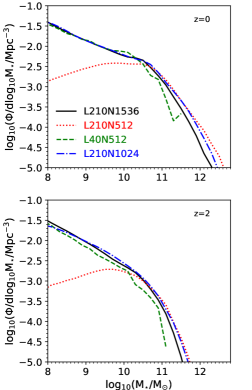
Figure 16: SMF at $z=0$ and $z=0$ for our default Shark model, run on the $4$ simulations of Table 5, as labelled.

An advantage of the SURFS simulations suite, is the possibility of testing the effect of resolution and simulated volume on galaxy properties. Table 5 shows the simulation parameters of all the SURFS run that were presented in Elahi et al. (2018). The parameters of our default Shark model (see values in Table 3) were chosen using the L210N1536 simulation. We fixed those parameters, and run the model on the other three simulations of Table 5 to assess the convergence of our results.

Fig. 16 shows the SMF at two redshifts for our default Shark model run on all the SURFS simulations. The low-mass end of the SMF at $z=0$ is well converged at the resolution level of the L210N1024 simulation. However, that is not the case at $z=2$, as the L210N1024 produces a flatter low-mass end compared to both the L210N1536 and L40N512 simulations. There is also a difference between L210N1536 and L40N512 in this regime, which may indicate that the L210N1536 is not well converged. At the massive end, we see that the poorer the resolution, the larger the stellar mass at fixed number density. This is due to the merger history of massive halos not being well converged. This affects massive galaxies more prominently as those are the ones whose growth is dominated by mergers (Robotham et al., 2014).

Fig. 17 shows the HI Mf at $z=0$ for our default Shark model run on all the SURFS simulations. The effect of resolution at the low-mass end here is more dramatic than for the SMF. Our default L210N1536 has an HI MF converged only at $M_{\rm HI}\gtrsim 10^{8}\,\rm M_{\odot}$ when we compare it with the higher resolution, smaller volume L40N512. At the high-mass end we see much better convergence than what we obtain for the SMF. This is because the galaxies with $M_{\rm HI}\gtrsim 10^{10}\,\rm M_{\odot}$ tend to be star-forming galaxies with stellar masses a few times $M_{\star}\sim 10^{10}\,\rm M_{\odot}$. Those live in halos of masses $10^{12}\rm\,M_{\odot}$, which are well converged at the resolution of all the SURFS runs.

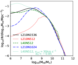
Figure 17: HI MF at $z=0$ for our default Shark model, run on the $4$ simulations of Table 5, as labelled.

The drop seen in the L40N512 between $10^{7}\,\rm M_{\odot}\lesssim M_{\rm HI}\lesssim 10^{8}\,\rm M_{\odot}$ is not due to resolution, but to the modelling of photo-ionisation feedback. To demonstrate that, we show as dotted, acqua-marine line a model variation adopting parameter values similar to those of Kim et al. (2015) for the Sobacchi & Mesinger (2013) model. The result is that the drop disappears, and instead we see a bump at at $M_{\rm HI}\approx 10^{7.7}\,\rm M_{\odot}$. Thus, the shape of the HI MF at the low-mass end is the result of a complex interplay between photo-ionisation feedback, the star formation law (via its effect on the amount of HI in satellite galaxies) and the resolution of the simulation.

References

- Andrews & Martini (2013) Andrews B. H., Martini P., 2013, ApJ, 765, 140
- Asplund et al. (2009) Asplund M., Grevesse N., Sauval A. J., Scott P., 2009, ARA&A, 47, 481
- Barkana & Loeb (2001) Barkana R., Loeb A., 2001, Phys. Rep., 349, 125
- Baugh et al. (1996) Baugh C. M., Cole S., Frenk C. S., 1996, MNRAS, 283, 1361
- Behroozi et al. (2013a) Behroozi P. S., Wechsler R. H., Conroy C., 2013a, ApJ, 770, 57
- Behroozi et al. (2013b) Behroozi P. S., Wechsler R. H., Wu H.-Y., 2013b, ApJ, 762, 109
- Benson (2012) Benson A. J., 2012, New A, 17, 175
- Benson (2014) —, 2014, MNRAS, 444, 2599
- Benson & Bower (2010) Benson A. J., Bower R., 2010, MNRAS, 405, 1573
- Benson et al. (2003) Benson A. J., Bower R. G., Frenk C. S., Lacey C. G., Baugh C. M., Cole S., 2003, ApJ, 599, 38
- Bernardi et al. (2013) Bernardi M., Meert A., Sheth R. K., Vikram V., Huertas-Company M., Mei S., Shankar F., 2013, MNRAS, 436, 697
- Blitz & Rosolowsky (2006) Blitz L., Rosolowsky E., 2006, ApJ, 650, 933
- Bolatto et al. (2017) Bolatto A. D., Chatterjee S., Casey C. M., Chomiuk L., de Pater I., Dickinson M., Di Francesco J., Hallinan G. et al, 2017, ArXiv:1711.09960
- Bolatto et al. (2013) Bolatto A. D., Wolfire M., Leroy A. K., 2013, ARA&A, 51, 207
- Bonatto & Bica (2011) Bonatto C., Bica E., 2011, MNRAS, 415, 2827
- Bondi (1952) Bondi H., 1952, MNRAS, 112, 195
- Booth et al. (2009) Booth R. S., de Blok W. J. G., Jonas J. L., Fanaroff B., 2009, ArXiv:0910.2935
- Boselli et al. (2014) Boselli A., Cortese L., Boquien M., Boissier S., Catinella B., Lagos C., Saintonge A., 2014, A&A, 564, A66
- Bournaud et al. (2011) Bournaud F., Chapon D., Teyssier R., Powell L. C., Elmegreen B. G., Elmegreen D. M., Duc P.-A., Contini T. et al, 2011, ApJ, 730, 4
- Bower et al. (2012) Bower R. G., Benson A. J., Crain R. A., 2012, MNRAS, 2860
- Bower et al. (2006) Bower R. G., Benson A. J., Malbon R., Helly J. C., Frenk C. S., Baugh C. M., Cole S., Lacey C. G., 2006, MNRAS, 370, 645
- Braun et al. (2009) Braun R., Thilker D. A., Walterbos R. A. M., Corbelli E., 2009, ApJ, 695, 937
- Brinchmann et al. (2004) Brinchmann J., Charlot S., White S. D. M., Tremonti C., Kauffmann G., Heckman T., Brinkmann J., 2004, MNRAS, 351, 1151
- Bromm & Larson (2004) Bromm V., Larson R. B., 2004, ARA&A, 42, 79
- Brown et al. (2015) Brown T., Catinella B., Cortese L., Kilborn V., Haynes M. P., Giovanelli R., 2015, MNRAS, 452, 2479
- Bullock et al. (2001) Bullock J. S., Dekel A., Kolatt T. S., Kravtsov A. V., Klypin A. A., Porciani C., Primack J. R., 2001, ApJ, 555, 240
- Cañas et al. (2018) Cañas R., Elahi P. J., Welker C., Lagos C. d. P., Power C., Dubois Y., Pichon C., 2018, ArXiv:1806.11417
- Calette et al. (2018) Calette A. R., Avila-Reese V., Rodríguez-Puebla A., Hernández-Toledo H., Papastergis E., 2018, ArXiv:1803.07692
- Catinella et al. (2018) Catinella B., Saintonge A., Janowiecki S., Cortese L., Davé R., Lemonias J. J., Cooper A. P., Schiminovich D. et al, 2018, MNRAS, 476, 875
- Ceverino et al. (2015) Ceverino D., Dekel A., Tweed D., Primack J., 2015, MNRAS, 447, 3291
- Chabrier (2003) Chabrier G., 2003, PASP, 115, 763
- Clauwens et al. (2018) Clauwens B., Schaye J., Franx M., Bower R. G., 2018, MNRAS, 478, 3994
- Cole & Lacey (1996) Cole S., Lacey C., 1996, MNRAS, 281, 716
- Cole et al. (2000) Cole S., Lacey C. G., Baugh C. M., Frenk C. S., 2000, MNRAS, 319, 168
- Conroy et al. (2009) Conroy C., Gunn J. E., White M., 2009, ApJ, 699, 486
- Contreras et al. (2017) Contreras S., Padilla N., Lagos C. D. P., 2017, MNRAS, 472, 4992
- Cora (2006) Cora S. A., 2006, MNRAS, 368, 1540
- Cora et al. (2018) Cora S. A., Vega-Martínez C. A., Hough T., Ruiz A. N., Orsi Á., Muñoz Arancibia A. M., Gargiulo I. D., Collacchioni F. et al, 2018, MNRAS
- Crain et al. (2015) Crain R. A., Schaye J., Bower R. G., Furlong M., Schaller M., Theuns T., Dalla Vecchia C., Frenk C. S. et al, 2015, MNRAS, 450, 1937
- Creasey et al. (2013) Creasey P., Theuns T., Bower R. G., 2013, MNRAS, 429, 1922
- Croton et al. (2006) Croton D. J., Springel V., White S. D. M., De Lucia G., Frenk C. S., Gao L., Jenkins A., Kauffmann G. et al, 2006, MNRAS, 365, 11
- Croton et al. (2016) Croton D. J., Stevens A. R. H., Tonini C., Garel T., Bernyk M., Bibiano A., Hodkinson L., Mutch S. J. et al, 2016, ApJS, 222, 22
- da Cunha et al. (2017) da Cunha E., Hopkins A. M., Colless M., Taylor E. N., Blake C., Howlett C., Magoulas C., Lucey J. R. et al, 2017, PASA, 34, e047
- Daddi et al. (2010a) Daddi E., Bournaud F., Walter F., Dannerbauer H., Carilli C. L., Dickinson M., Elbaz D., Morrison G. E. et al, 2010a, ApJ, 713, 686
- Daddi et al. (2010b) Daddi E., Elbaz D., Walter F., Bournaud F., Salmi F., Carilli C., Dannerbauer H., Dickinson M. et al, 2010b, ApJ, 714, L118
- Davé et al. (2012) Davé R., Finlator K., Oppenheimer B. D., 2012, MNRAS, 421, 98
- Davies et al. (2016) Davies L. J. M., Driver S. P., Robotham A. S. G., Grootes M. W., Popescu C. C., Tuffs R. J., Hopkins A., Alpaslan M. et al, 2016, MNRAS, 461, 458
- Decarli et al. (2016) Decarli R., Walter F., Aravena M., Carilli C., Bouwens R., da Cunha E., Daddi E., Ivison R. J. et al, 2016, ApJ, 833, 69
- Driver et al. (2018) Driver S. P., Andrews S. K., da Cunha E., Davies L. J., Lagos C., Robotham A. S. G., Vinsen K., Wright A. H. et al, 2018, MNRAS, 475, 2891
- Driver et al. (2016) Driver S. P., Davies L. J., Meyer M., Power C., Robotham A. S. G., Baldry I. K., Liske J., Norberg P., 2016, The Universe of Digital Sky Surveys, 42, 205
- Duffy et al. (2012) Duffy A. R., Moss A., Staveley-Smith L., 2012, PASA, 29, 202
- Duffy et al. (2008) Duffy A. R., Schaye J., Kay S. T., Dalla Vecchia C., 2008, MNRAS, 390, L64
- Dutton & Macciò (2014) Dutton A. A., Macciò A. V., 2014, MNRAS, 441, 3359
- Efstathiou et al. (1982) Efstathiou G., Lake G., Negroponte J., 1982, MNRAS, 199, 1069
- Einasto (1965) Einasto J., 1965, Trudy Astrofizicheskogo Instituta Alma-Ata, 5, 87
- Elahi et al. (2013) Elahi P. J., Han J., Lux H., Ascasibar Y., Behroozi P., Knebe A., Muldrew S. I., Onions J. et al, 2013, MNRAS, 433, 1537
- Elahi et al. (2017) Elahi P. J., Power C., Lagos C. d. P., Poulton R., Robotham A. S. G., 2017, ArXiv:1712.01989
- Elahi et al. (2011) Elahi P. J., Thacker R. J., Widrow L. M., 2011, MNRAS, 418, 320
- Elahi et al. (2018) Elahi P. J., Welker C., Power C., del P Lagos C., Robotham A. S. G., Cañas R., Poulton R., 2018, MNRAS
- Elmegreen (1989) Elmegreen B. G., 1989, ApJ, 338, 178
- Ferland et al. (1998) Ferland G. J., Korista K. T., Verner D. A., Ferguson J. W., Kingdon J. B., Verner E. M., 1998, PASP, 110, 761
- Fu et al. (2010) Fu J., Guo Q., Kauffmann G., Krumholz M. R., 2010, MNRAS, 409, 515
- Gallazzi et al. (2005) Gallazzi A., Charlot S., Brinchmann J., White S. D. M., Tremonti C. A., 2005, MNRAS, 362, 41
- Gardner et al. (2006) Gardner J. P., Mather J. C., Clampin M., Doyon R., Greenhouse M. A., Hammel H. B., Hutchings J. B., Jakobsen P., Lilly S. J., Long K. S., Lunine J. I., McCaughrean M. J., Mountain M., Nella J., Rieke G. H., Rieke M. J., Rix H.-W., Smith E. P., Sonneborn G., Stiavelli M., Stockman H. S., Windhorst R. A., Wright G. S., 2006, in Proc. SPIE, Vol. 6265, Society of Photo-Optical Instrumentation Engineers (SPIE) Conference Series, p. 62650N
- Genzel et al. (2015) Genzel R., Tacconi L. J., Lutz D., Saintonge A., Berta S., Magnelli B., Combes F., García-Burillo S. et al, 2015, ApJ, 800, 20
- Gnedin (2012) Gnedin N. Y., 2012, ApJ, 754, 113
- Gnedin & Draine (2014) Gnedin N. Y., Draine B. T., 2014, ApJ, 795, 37
- Gnedin & Kravtsov (2011) Gnedin N. Y., Kravtsov A. V., 2011, ApJ, 728, 88
- Gonzalez-Perez et al. (2014) Gonzalez-Perez V., Lacey C. G., Baugh C. M., Lagos C. D. P., Helly J., Campbell D. J. R., Mitchell P. D., 2014, MNRAS
- Guo et al. (2015) Guo K., Zheng X. Z., Wang T., Fu H., 2015, ApJ, 808, L49
- Guo et al. (2016) Guo Q., Gonzalez-Perez V., Guo Q., Schaller M., Furlong M., Bower R. G., Cole S., Crain R. A. et al, 2016, MNRAS, 461, 3457
- Guo et al. (2011) Guo Q., White S., Boylan-Kolchin M., De Lucia G., Kauffmann G., Lemson G., Li C., Springel V. et al, 2011, MNRAS, 413, 101
- Haardt & Madau (2012) Haardt F., Madau P., 2012, ApJ, 746, 125
- Häring & Rix (2004) Häring N., Rix H.-W., 2004, ApJ, 604, L89
- Haynes et al. (2018) Haynes M. P., Giovanelli R., Kent B. R., Adams E. A. K., Balonek T. J., Craig D. W., Fertig D., Finn R. et al, 2018, ArXiv:1805.11499
- Henriques et al. (2009) Henriques B. M. B., Thomas P. A., Oliver S., Roseboom I., 2009, MNRAS, 396, 535
- Henriques et al. (2015) Henriques B. M. B., White S. D. M., Thomas P. A., Angulo R., Guo Q., Lemson G., Springel V., Overzier R., 2015, MNRAS, 451, 2663
- Henriques et al. (2013) Henriques B. M. B., White S. D. M., Thomas P. A., Angulo R. E., Guo Q., Lemson G., Springel V., 2013, MNRAS, 431, 3373
- Hirschmann et al. (2016) Hirschmann M., De Lucia G., Fontanot F., 2016, MNRAS, 461, 1760
- Hopkins et al. (2009) Hopkins P. F., Hernquist L., Cox T. J., Keres D., Wuyts S., 2009, ApJ, 691, 1424
- Hopkins et al. (2012a) Hopkins P. F., Narayanan D., Murray N., Quataert E., 2012a, ArXiv:1209.0459
- Hopkins et al. (2012b) Hopkins P. F., Quataert E., Murray N., 2012b, MNRAS, 421, 3522
- Jiang et al. (2014) Jiang L., Helly J. C., Cole S., Frenk C. S., 2014, MNRAS, 440, 2115
- Johnston et al. (2008) Johnston S., Taylor R., Bailes M., Bartel N., Baugh C., Bietenholz M., Blake C., Braun R. et al, 2008, Experimental Astronomy, 22, 151
- Jones et al. (2018) Jones M. G., Haynes M. P., Giovanelli R., Moorman C., 2018, MNRAS, 477, 2
- Kalirai (2018) Kalirai J., 2018, Contemporary Physics, 59, 251
- Karim et al. (2011) Karim A., Schinnerer E., Martínez-Sansigre A., Sargent M. T., van der Wel A., Rix H.-W., Ilbert O., Smolčić V. et al, 2011, ApJ, 730, 61
- Kauffmann et al. (1999) Kauffmann G., Colberg J. M., Diaferio A., White S. D. M., 1999, MNRAS, 303, 188
- Kauffmann & Haehnelt (2000) Kauffmann G., Haehnelt M., 2000, MNRAS, 311, 576
- Keres et al. (2003) Keres D., Yun M. S., Young J. S., 2003, ApJ, 582, 659
- Kewley & Ellison (2008) Kewley L. J., Ellison S. L., 2008, ApJ, 681, 1183
- Kim et al. (2015) Kim H.-S., Wyithe J. S. B., Power C., Park J., Lagos C. d. P., Baugh C. M., 2015, MNRAS, 453, 2315
- Kirby et al. (2013) Kirby E. N., Cohen J. G., Guhathakurta P., Cheng L., Bullock J. S., Gallazzi A., 2013, ApJ, 779, 102
- Knebe et al. (2017) Knebe A., Pearce F. R., Gonzalez-Perez V., Thomas P. A., Benson A., Asquith R., Blaizot J., Bower R. et al, 2017, ArXiv:1712.06420
- Kormendy & Kennicutt (2004) Kormendy J., Kennicutt Jr. R. C., 2004, ARA&A, 42, 603
- Kregel et al. (2002) Kregel M., van der Kruit P. C., de Grijs R., 2002, MNRAS, 334, 646
- Krumholz (2013) Krumholz M. R., 2013, MNRAS, 436, 2747
- Krumholz & McKee (2005) Krumholz M. R., McKee C. F., 2005, ApJ, 630, 250
- Krumholz et al. (2009) Krumholz M. R., McKee C. F., Tumlinson J., 2009, ApJ, 699, 850
- Lacey & Cole (1993) Lacey C., Cole S., 1993, MNRAS, 262, 627
- Lacey et al. (2016) Lacey C. G., Baugh C. M., Frenk C. S., Benson A. J., Bower R. G., Cole S., Gonzalez-Perez V., Helly J. C. et al, 2016, MNRAS, 462, 3854
- Lagos et al. (2011a) Lagos C. D. P., Baugh C. M., Lacey C. G., Benson A. J., Kim H.-S., Power C., 2011a, MNRAS, 418, 1649
- Lagos et al. (2014a) Lagos C. D. P., Baugh C. M., Zwaan M. A., Lacey C. G., Gonzalez-Perez V., Power C., Swinbank A. M., van Kampen E., 2014a, MNRAS, 440, 920
- Lagos et al. (2015) Lagos C. d. P., Crain R. A., Schaye J., Furlong M., Frenk C. S., Bower R. G., Schaller M., Theuns T. et al, 2015, MNRAS, 452, 3815
- Lagos et al. (2014b) Lagos C. d. P., Davis T. A., Lacey C. G., Zwaan M. A., Baugh C. M., Gonzalez-Perez V., Padilla N. D., 2014b, MNRAS, 443, 1002
- Lagos et al. (2013) Lagos C. d. P., Lacey C. G., Baugh C. M., 2013, MNRAS, 436, 1787
- Lagos et al. (2011b) Lagos C. D. P., Lacey C. G., Baugh C. M., Bower R. G., Benson A. J., 2011b, MNRAS, 416, 1566
- Lagos et al. (2009) Lagos C. D. P., Padilla N. D., Cora S. A., 2009, MNRAS, 395, 625
- Lagos et al. (2018a) Lagos C. d. P., Schaye J., Bahé Y., Van de Sande J., Kay S. T., Barnes D., Davis T. A., Dalla Vecchia C., 2018a, MNRAS, 476, 4327
- Lagos et al. (2018b) Lagos C. d. P., Stevens A. R. H., Bower R. G., Davis T. A., Contreras S., Padilla N. D., Obreschkow D., Croton D. et al, 2018b, MNRAS, 473, 4956
- Lagos et al. (2016) Lagos C. d. P., Theuns T., Schaye J., Furlong M., Bower R. G., Schaller M., Crain R. A., Trayford J. W. et al, 2016, MNRAS, 459, 2632
- Lange et al. (2016) Lange R., Moffett A. J., Driver S. P., Robotham A. S. G., Lagos C. d. P., Kelvin L. S., Conselice C., Margalef-Bentabol B. et al, 2016, MNRAS, 462, 1470
- Lemonias et al. (2013) Lemonias J. J., Schiminovich D., Catinella B., Heckman T. M., Moran S. M., 2013, ArXiv:1308.2178
- Leroy et al. (2008) Leroy A. K., Walter F., Brinks E., Bigiel F., de Blok W. J. G., Madore B., Thornley M. D., 2008, AJ, 136, 2782
- Leroy et al. (2013) Leroy A. K., Walter F., Sandstrom K., Schruba A., Munoz-Mateos J.-C., Bigiel F., Bolatto A., Brinks E. et al, 2013, AJ, 146, 19
- Li & White (2009) Li C., White S. D. M., 2009, MNRAS, 398, 2177
- Lu et al. (2011) Lu Y., Mo H. J., Weinberg M. D., Katz N., 2011, MNRAS, 416, 1949
- Marchesini et al. (2009) Marchesini D., van Dokkum P. G., Förster Schreiber N. M., Franx M., Labbé I., Wuyts S., 2009, ApJ, 701, 1765
- McAlpine et al. (2015) McAlpine S., Helly J. C., Schaller M., Trayford J. W., Qu Y., Furlong M., Bower R. G., Crain R. A. et al, 2015, ArXiv:1510.01320
- McConnell & Ma (2013) McConnell N. J., Ma C.-P., 2013, ApJ, 764, 184
- Meyer et al. (2004) Meyer M. J., Zwaan M. A., Webster R. L., Staveley-Smith L., Ryan-Weber E., Drinkwater M. J., Barnes D. G., Howlett M. et al, 2004, MNRAS, 350, 1195
- Mitchell et al. (2013) Mitchell P. D., Lacey C. G., Baugh C. M., Cole S., 2013, ArXiv:1303.7228
- Mitchell et al. (2016) —, 2016, MNRAS, 456, 1459
- Mitchell et al. (2014) Mitchell P. D., Lacey C. G., Cole S., Baugh C. M., 2014, MNRAS, 444, 2637
- Mitchell et al. (2018) Mitchell P. D., Lacey C. G., Lagos C. D. P., Frenk C. S., Bower R. G., Cole S., Helly J. C., Schaller M. et al, 2018, MNRAS, 474, 492
- Mo et al. (1998) Mo H. J., Mao S., White S. D. M., 1998, MNRAS, 295, 319
- Moffett et al. (2016) Moffett A. J., Lange R., Driver S. P., Robotham A. S. G., Kelvin L. S., Alpaslan M., Andrews S. K., Bland-Hawthorn J. et al, 2016, MNRAS, 462, 4336
- Moster et al. (2013) Moster B. P., Naab T., White S. D. M., 2013, MNRAS, 428, 3121
- Moustakas et al. (2013) Moustakas J., Coil A. L., Aird J., Blanton M. R., Cool R. J., Eisenstein D. J., Mendez A. J., Wong K. C. et al, 2013, ApJ, 767, 50
- Muratov et al. (2015) Muratov A. L., Kereš D., Faucher-Giguère C.-A., Hopkins P. F., Quataert E., Murray N., 2015, MNRAS, 454, 2691
- Murray et al. (2013) Murray S. G., Power C., Robotham A. S. G., 2013, Astronomy and Computing, 3, 23
- Mutch et al. (2016) Mutch S. J., Geil P. M., Poole G. B., Angel P. W., Duffy A. R., Mesinger A., Wyithe J. S. B., 2016, MNRAS, 462, 250
- Muzzin et al. (2013) Muzzin A., Marchesini D., Stefanon M., Franx M., McCracken H. J., Milvang-Jensen B., Dunlop J. S., Fynbo J. P. U. et al, 2013, ApJ, 777, 18
- Nulsen & Fabian (2000) Nulsen P. E. J., Fabian A. C., 2000, MNRAS, 311, 346
- Obreschkow et al. (2009) Obreschkow D., Heywood I., Klöckner H.-R., Rawlings S., 2009, ApJ, 702, 1321
- Okamoto et al. (2008) Okamoto T., Gao L., Theuns T., 2008, MNRAS, 390, 920
- Ostriker et al. (2010) Ostriker E. C., McKee C. F., Leroy A. K., 2010, ApJ, 721, 975
- Ostriker & Peebles (1973) Ostriker J. P., Peebles P. J. E., 1973, ApJ, 186, 467
- Parkash et al. (2018) Parkash V., Brown M. J. I., Jarrett T. H., Bonne N. J., 2018, ArXiv:1807.06246
- Pillepich et al. (2018) Pillepich A., Springel V., Nelson D., Genel S., Naiman J., Pakmor R., Hernquist L., Torrey P. et al, 2018, MNRAS, 473, 4077
- Planck Collaboration et al. (2016) Planck Collaboration, Ade P. A. R., Aghanim N., Arnaud M., Ashdown M., Aumont J., Baccigalupi C., Banday A. J. et al, 2016, A&A, 594, A13
- Popping et al. (2014) Popping G., Pérez-Beaupuits J. P., Spaans M., Trager S. C., Somerville R. S., 2014, MNRAS, 444, 1301
- Rhee et al. (2018) Rhee J., Lah P., Briggs F. H., Chengalur J. N., Colless M., Willner S. P., Ashby M. L. N., Le Fèvre O., 2018, MNRAS, 473, 1879
- Robotham et al. (2014) Robotham A. S. G., Driver S. P., Davies L. J. M., Hopkins A. M., Baldry I. K., Agius N. K., Bauer A. E., Bland-Hawthorn J. et al, 2014, MNRAS, 444, 3986
- Robotham & Howlett (2018) Robotham A. S. G., Howlett C., 2018, Research Notes of the American Astronomical Society, 2, 55
- Robotham et al. (2017) Robotham A. S. G., Taranu D. S., Tobar R., Moffett A., Driver S. P., 2017, MNRAS, 466, 1513
- Romeo & Wiegert (2011) Romeo A. B., Wiegert J., 2011, MNRAS, 416, 1191
- Ruiz et al. (2015) Ruiz A. N., Cora S. A., Padilla N. D., Domínguez M. J., Vega-Martínez C. A., Tecce T. E., Orsi Á., Yaryura Y. et al, 2015, ApJ, 801, 139
- Saintonge et al. (2017) Saintonge A., Catinella B., Tacconi L. J., Kauffmann G., Genzel R., Cortese L., Davé R., Fletcher T. J. et al, 2017, ApJS, 233, 22
- Santini et al. (2012) Santini P., Fontana A., Grazian A., Salimbeni S., Fontanot F., Paris D., Boutsia K., Castellano M. et al, 2012, A&A, 538, A33
- Schaye et al. (2015) Schaye J., Crain R. A., Bower R. G., Furlong M., Schaller M., Theuns T., Dalla Vecchia C., Frenk C. S. et al, 2015, MNRAS, 446, 521
- Schaye et al. (2010) Schaye J., Dalla Vecchia C., Booth C. M., Wiersma R. P. C., Theuns T., Haas M. R., Bertone S., Duffy A. R. et al, 2010, MNRAS, 402, 1536
- Schilizzi et al. (2008) Schilizzi R. T., Dewdney P. E. F., Lazio T. J. W., 2008, in Society of Photo-Optical Instrumentation Engineers (SPIE) Conference Series, Vol. 7012, Society of Photo-Optical Instrumentation Engineers (SPIE) Conference Series
- Scoville et al. (2016) Scoville N., Sheth K., Aussel H., Vanden Bout P., Capak P., Bongiorno A., Casey C. M., Murchikova L. et al, 2016, ApJ, 820, 83
- Shattow & Croton (2015) Shattow G. M., Croton D. J., 2015, MNRAS, 452, 1779
- Sheth et al. (2001) Sheth R. K., Mo H. J., Tormen G., 2001, MNRAS, 323, 1
- Shull et al. (2012) Shull J. M., Smith B. D., Danforth C. W., 2012, ApJ, 759, 23
- Simha & Cole (2017) Simha V., Cole S., 2017, MNRAS, 472, 1392
- Sobacchi & Mesinger (2013) Sobacchi E., Mesinger A., 2013, MNRAS, 432, L51
- Somerville & Davé (2015) Somerville R. S., Davé R., 2015, ARA&A, 53, 51
- Somerville et al. (2015) Somerville R. S., Popping G., Trager S. C., 2015, MNRAS, 453, 4337
- Springel et al. (2005) Springel V., White S. D. M., Jenkins A., Frenk C. S., Yoshida N., Gao L., Navarro J., Thacker R. et al, 2005, Nature, 435, 629
- Springel et al. (2001) Springel V., White S. D. M., Tormen G., Kauffmann G., 2001, MNRAS, 328, 726
- Stevens et al. (2016) Stevens A. R. H., Croton D. J., Mutch S. J., 2016, MNRAS, 461, 859
- Stringer & Benson (2007) Stringer M. J., Benson A. J., 2007, MNRAS, 382, 641
- Sutherland & Dopita (1993) Sutherland R. S., Dopita M. A., 1993, ApJS, 88, 253
- Swinbank et al. (2017) Swinbank A. M., Harrison C. M., Trayford J., Schaller M., Smail I., Schaye J., Theuns T., Smit R. et al, 2017, MNRAS, 467, 3140
- Tacconi et al. (2018) Tacconi L. J., Genzel R., Saintonge A., Combes F., García-Burillo S., Neri R., Bolatto A., Contini T. et al, 2018, ApJ, 853, 179
- Tremonti et al. (2004) Tremonti C. A., Heckman T. M., Kauffmann G., Brinchmann J., Charlot S., White S. D. M., Seibert M., Peng E. W. et al, 2004, ApJ, 613, 898
- van de Voort et al. (2012) van de Voort F., Schaye J., Altay G., Theuns T., 2012, MNRAS, 421, 2809
- Wang et al. (2015) Wang L., Dutton A. A., Stinson G. S., Macciò A. V., Penzo C., Kang X., Keller B. W., Wadsley J., 2015, MNRAS, 454, 83
- Wellons et al. (2016) Wellons S., Torrey P., Ma C.-P., Rodriguez-Gomez V., Pillepich A., Nelson D., Genel S., Vogelsberger M. et al, 2016, MNRAS, 456, 1030
- Wellons et al. (2015) Wellons S., Torrey P., Ma C.-P., Rodriguez-Gomez V., Vogelsberger M., Kriek M., van Dokkum P., Nelson E. et al, 2015, MNRAS, 449, 361
- White & Rees (1978) White S. D. M., Rees M. J., 1978, MNRAS, 183, 341
- Willett et al. (2015) Willett K. W., Schawinski K., Simmons B. D., Masters K. L., Skibba R. A., Kaviraj S., Melvin T., Wong O. I. et al, 2015, MNRAS, 449, 820
- Wolfire et al. (2003) Wolfire M. G., McKee C. F., Hollenbach D., Tielens A. G. G. M., 2003, ApJ, 587, 278
- Wootten & Thompson (2009) Wootten A., Thompson A. R., 2009, IEEE Proceedings, 97, 1463
- Wright et al. (2017) Wright A. H., Robotham A. S. G., Driver S. P., Alpaslan M., Andrews S. K., Baldry I. K., Bland-Hawthorn J., Brough S. et al, 2017, MNRAS, 470, 283
- Xie et al. (2017) Xie L., De Lucia G., Hirschmann M., Fontanot F., Zoldan A., 2017, MNRAS, 469, 968
- Yates et al. (2013) Yates R. M., Henriques B., Thomas P. A., Kauffmann G., Johansson J., White S. D. M., 2013, MNRAS, 435, 3500
- Zoldan et al. (2018) Zoldan A., De Lucia G., Xie L., Fontanot F., Hirschmann M., 2018, ArXiv:1803.08056
- Zolotov et al. (2015) Zolotov A., Dekel A., Mandelker N., Tweed D., Inoue S., DeGraf C., Ceverino D., Primack J. R. et al, 2015, MNRAS, 450, 2327
- Zwaan et al. (2005) Zwaan M. A., Meyer M. J., Staveley-Smith L., Webster R. L., 2005, MNRAS, 359, L30