NMT-based Cross-lingual Document Embeddings

Abstract

This paper investigates a cross-lingual document embedding method that improves the current Neural machine Translation framework based Document Vector (NTDV or simply NV). NV is developed with a self-attention mechanism under the neural machine translation (NMT) framework. In NV, each pair of parallel documents in different languages are projected to the same shared layer in the model. However, the pair of NV embeddings are not guaranteed to be similar. This paper further adds a distance constraint to the training objective function of NV so that the two embeddings of a parallel document are required to be as close as possible. The new method will be called constrained NV (cNV). In a cross-lingual document classification task, the new cNV performs as well as NV and outperforms other published studies that require forward-pass decoding. Compared with the previous NV, cNV does not need a translator during testing, and so the method is lighter and more flexible.

Index Terms: cross-lingual document representation

1 Introduction

Cross-lingual embedding of texts from different languages to a unified space will enable comparison and knowledge-sharing between languages [1, 2, 3, 4, 5, 6, 7, 8, 9]. With cross-lingual embedding, data in resource-rich languages can be used to help understand inputs from resource-scarce languages. Prior works can be categorized into cross-lingual word embedding [10, 11, 2, 4] and cross-lingual text (document/sentence) embedding [1, 12, 3, 4]. In this study, a cross-lingual document/sentence vectorization model for cross-lingual text embedding is developed under a self-attentive neural machine-translation (NMT) framework with a distance constraint (cNTDV, or cNV for short). cNV is improved from a recent method called neural machine translation framework based document vector (NTDV, or NV for short) [13] with an additional constraint to minimize the distance between their two embedding vectors produced from each parallel document. Whereas an NV in a cross-lingual task is formed by combining the two embeddings of a document in its source language and its translated language, these two embeddings produced by our new cNV method are so similar that, in the production mode, only one is needed (as using both gives only small additional performance gain). Thus, there is an option of using or not using the extra translation step. (NV needs a translator to produce translated text in order to form a joint vector for an application). For better performance (accuracy), the translator could be used; for faster performance, the translator can be removed and the performance is still superior to many traditional forward-propagation methods. cNV is more flexible and lightweight for applications. Note that the aforementioned translator is trained with the same Europarl corpora as in previous research. Moreover, we also study the effectiveness of distance constraint training by visualizing the manifold projection of various NV and cNV embedding.

The cross-lingual document classification task on RCV1/RCV2 was used to evaluate the effectiveness of the cNV model [14, 10]. If the cross-lingual document embedding method is successful, the classifier (e.g., SVM) trained on 1K English embeddings would be able to classify the 5K German embeddings in the test set as well. Note that the embedding models were pre-trained on the Europarl v7 parallel corpus which is unrelated to this classification task. This design reflects the reality that tasks unrelated parallel data is easy to find while task-related user data for a new language is harder to obtain. The embedding model is not fine-tuned using any testing or training data in the RCV1/RCV2 dataset. This is inherently different from the task-unrelated pre-training and task-specific fine-tuning framework like XLNet [15]. Albeit the pre-training and fine-tuning framework would normally produce better performance with encoder and classifier optimized together in a complete network, in many NLP applications, it is more convenient to have a readily available pre-trained embedding without fine-tuning so a single uniform embedding can be swiftly plugged into many different applications, such as comparison, clustering or indexing. It would be much easier to compare or index uniformed embedding vectors across tasks than the different encoder outputs fine-tuned in each task.

There are also NMT based approaches like LASER [16, 17], where the cross-lingual embedding can be obtained by using a uniform dictionary, shared encoder, and shared target languages without using a distance constraint. However, one motivation of the cNV and NV model is that we can easily convert the models from a pair of existing NMT models. Shared encoder and uniform dictionary setup are used in multi-lingual translation models which are rare to find. Most existing NMT models only translate between two languages. A pair of NMT models normally would have different encoder/decoder and dictionary indexing, so we have to assume that they are not shareable. Therefore, NV and cNV would use independent encoders and dictionaries in different translation directions. When training the cNV and NV, we only need to copy the encoder and decoder parameters from a pair of NMT models and then adapt the shared layers with a few iterations. Moreover, after pre-training, we can also use the existing NMT models to boost the performance of our model as mentioned in the previous paragraph. Finally, the uniform dictionary in LASER would multiply the input/output layer size by the number of languages the multi-lingual translation model includes. Fully sharing an encoder/decoder across different language families (e.g. Chinese and English) could potentially cause a drop of performance in a multi-lingual model [18]. A LASER-like framework is more suitable for a large number of languages while NV and cNV are designed to be easily adapted from pre-trained NMT models which are abundantly available. Note that the pre-trained encoder provided in LASER [16, 17] is a much deeper model and is trained with far more data than the standard Europarl corpus which is used in this study and many previous studies.

(a) In training, English inputs pass through the left NMT_en→de, while German inputs pass through the right NMT_de→en.

(b) Producing cNV${{}_{\star}^{(en)}}\thinspace$and NV${{}_{\star}^{(en)}}\thinspace$with English (left) or German (right) input texts. German input is first translated to English to produce $\mathbf{P}^{(en)}$.

(c) cNV${{}_{\star}^{(y)}}\thinspace$is cNV${{}_{\star}^{(en)}}\thinspace$if the input is English (left). cNV${{}_{\star}^{(y)}}\thinspace$is cNV${{}_{\star}^{(de)}}\thinspace$if the input is German (right). No translation is needed.

(d) Producing NV_:  , NV${{}_{sum}}\thinspace$, cNV${{}_{sum}}\thinspace$and cNV${{}_{con}}\thinspace$when input text is English. $\mathbf{P}^{(en)}$ and $\mathbf{P}^{(de)}$ are combined to obtain the final document vector.

Figure 1: The differences between various NV and cNV document vectors in training and production modes.

2 Model architecture

2.1 The attention-based NMT model

The cNV model is built on the NMT framework, which consists of an encoder-decoder structure with an attention mechanism [19]. cNV shares many similarities with a bilingual NMT model. It has two NMT models (NMT_a→b and NMT_b→a) in opposite directions, where $a\rightarrow b$ indicates the translation from source language $a$ to target language $b$. Shared layers are then inserted between the encoders and decoders. Fig. 1(a) shows the cNV model in the training mode with $a$ being English (en) and $b$ being German (de). NMT_a→b and NMT_b→a are first trained independently. Then their parameters are copied into the cNV model and are fixed in subsequent cNV training, in which only the parameters of the shared layers are updated. Given a pair of English and German sentences, the English sentence will be processed through the encoder of NMT_en→de, the shared layers, and its decoder resulting in the translation loss of $l_{mt}^{en\rightarrow de}$. Similarly, the German sentence in the pair will be processed through the encoder of NMT_de→en, the same shared layers, and its decoder resulting in the translation loss of $l_{mt}^{de\rightarrow en}$.

Previous researches show that the information from the encoder helps decide the content of the translated text — the adequacy [20, 21]. The NV model uses a multi-head self-attentive mechanism to summarize the adequacy information, taking advantage of the information extraction ability of the self-attention layer. This self-attention layer focuses only on the overall sequential pattern, in contrast to the self-attention mechanism in the transformer network that puts more weight on the time-sensitive-information [22]. It summarizes the input sequence to a fixed-length matrix (which becomes the document representation after some post-processing). Let $\bm{{z}}_{i}$ be the hidden state of the shared GRU layer. The context vector $\bm{{p}}_{m}$ produced by the $m$th attention head is given by:

$$g^{m}_{i}\!\!\! =\!\! f\left(\frac{(\mathbf{W}_{q}^{m}\bm{{z_{i}}}+\bm{{b}}_{q}^{m})^{T}(\mathbf{W}_{k}^{m}\bm{{z_{i}}}+\bm{{b}}_{k}^{m})}{\sqrt{d_{h}}}\right)$$ (1)

$$\bm{{p}}_{m}\!\!\! =\!\!\!\! \sum_{i=1}^{L_{x}}g^{m}_{i}(\mathbf{W}_{v}^{m}\bm{{z_{i}}}+\bm{{b}}_{v}^{m})$$ (2)

where $f(\cdot)$ is the softmax function; $i$ is the input word index; $\mathbf{W}_{q}^{m}$, $\mathbf{W}_{k}^{m}$, $\mathbf{W}_{v}^{m}$ and $\bm{{b}}_{q}^{m}$, $\bm{{b}}_{k}^{m}$, $\bm{{b}}_{v}^{m}$ are model parameters of the $m$th attention head, and the subscripts $q$, $k$, $v$ indicate the role of query, key and values in the attention mechanism [22], respectively; $d_{h}$ is the hidden layer size; $L_{x}$ is the length of input sentence.

Let there be $r$ attention heads, and $\mathbf{P}^{(a)}$ and $\mathbf{P}^{(b)}$ be the context matrix $\mathbf{P}$ from NMT_a→b and NMT_b→a, respectively, in which the $m$th column vector represents the context vector from the $m$th head. Different document/sentence vectors can be extracted by summing or concatenating the column vectors in $\mathbf{P}^{(a)}$ and/or $\mathbf{P}^{(b)}$ as follows:

$$\mathrm{cNV}^{(a)}_{sum}\! =\! \sum_{i=1}^{r}\bm{{p}}_{i}^{\ (a)}$$ (3)

$$\mathrm{cNV}_{sum}\! =\! \mathrm{cNV}^{(a)}_{sum}+\mathrm{cNV}^{(b)}_{sum}$$ (4)

$$\mathrm{cNV}^{(a)}_{con}\! =\! concat(\bm{{p}}_{1}^{\ (a)},\bm{{p}}_{2}^{\ (a)},\ldots,\bm{{p}}_{r}^{\ (a)})$$ (5)

$$\mathrm{cNV}_{con}\! =\! \mathrm{cNV}^{(a)}_{con}+\mathrm{cNV}^{(b)}_{con}\$$ (6)

where $\bm{{p}}_{i}^{\ (a)}$ and $\bm{{p}}_{i}^{\ (b)}$ are the $i$th column of $\mathbf{P}^{(a)}$ and $\mathbf{P}^{(b)}$, respectively, and $concat()$ is vector concatenation. Moreover, any operation for language $a$ also applies to language $b$.

2.2 Training with a distance constraint

Unlike the NV model in [13], we would like to have cNV${{}_{\star}^{(y)}}\thinspace$(where the $y$ ($any$) superscript indicates either $en$ or $de$ language, see Fig. 1(c)); The $\mathbf{P}^{(en)}$ and $\mathbf{P}^{(de)}$ produced by our new cNV model for the same document in either language of a language pair are to be very similar, so that one may use either one or both of them for cross-lingual tasks. To do that, a distance cost is added to the training cost function. The idea is to minimize the distance between related sentence pairs {$\mathbf{P}^{(a)}$, $\mathbf{P}^{(b)}$} while maximizing the distance between unrelated sentence pairs {$\mathbf{P}^{(a)}$, $\mathbf{P}^{(b_{j})}$}, where $\mathbf{P}^{(b_{j})}$ is the context matrix obtained from a randomly sampled $j$th sentence [1]. The distance cost with one negative sample is:

$$l_{d_{j}}=\max(0,\alpha+\alpha\frac{k_{d_{j}}}{2*v_{norm}+1})\ ,$$ (7)

where

$$k_{d_{j}}=|\mathbf{P}^{(a)}-\mathbf{P}^{(b)}|^{2}-|\mathbf{P}^{(a)}-\mathbf{P}^{(b_{j})}|^{2}\ ,$$ (8)

$\alpha$ is the margin and $|\cdot|$ is the Frobenius norm of a matrix; $v_{norm}$ is the average Frobenius norm of vectors in the training batch, ‘+1’ is to prevent division by zero . Finally, the total cost of the model is the sum of the distance costs from $N_{s}$ samplings plus the translation cost:

$$l_{com}=\beta\sum_{j=1}^{N_{s}}{l_{d_{j}}}+(1-\beta)(l_{mt}^{\ a\rightarrow b}+l_{mt}^{\ b\rightarrow a})\ ,$$ (9)

where $l_{mt}^{\ a\rightarrow b}$ and $l_{mt}^{\ b\rightarrow a}$ are the cross-entropy losses of the outputs from NMT_a→b and NMT_b→a, respectively. $0\leq\beta\leq 1$ is a weight to balance the translation cost and the distance cost. This novel cost function ensures that the produced document vectors contain ample semantic information and are, at the same time, very similar for parallel documents in a language pair.

Fig. 1 shows the production of various NV/cNV vectors. The main difference between them is that the translator is necessary in the previous NV model but is optional in the cNV model. In comparison with NV${{}_{\star}^{(en)}}\thinspace$, NV${{}_{\star}^{(de)}}\thinspace$and NV${{}_{\star}}\thinspace$, this paper’s cNV${{}_{\star}^{(y)}}\thinspace$do not use NMT translators. Instead, cNV${{}_{\star}^{(y)}}\thinspace$only use the NMT_en→de encoder for English inputs and the NMT_de→en encoder for German inputs. The corresponding NV${{}_{\star}^{(y)}}\thinspace$would have a very bad performance since NV${{}_{\star}^{(en)}}\thinspace$and NV${{}_{\star}^{(de)}}\thinspace$from the same document are not guaranteed to be similar.

3 Experiments

Table 1: The setting of various vectors in the cNV model.

Feature	Dimension	$r$	$d_{h}$
cNV${{}_{sum}}\thinspace$	1024	4	1024
cNV${{}_{sum}^{(y)}}\thinspace$	1024	4	1024
cNV${{}_{con}}\thinspace$	4096	4	1024
cNV${{}_{con}^{(y)}}\thinspace$	4096	4	1024

Our embedding model was trained on the Europarl v7 parallel corpus [23]. For training the attention-based NMT models and cNV, we adopt the same settings as in [13] with the following additional settings due to the distance constraint: $d_{h}=1024$, $r=4$, $N_{s}=20$, $\beta=0.5$, $\alpha=2\sqrt{d_{h}}$. In training the attention-based NMT models, we use the default setting with a mini-batch size of 80, a vocabulary size of 85,000, a maximum sentence length of 50, word embedding size of 500, and hidden layer size of 1024. The models are trained with the Adam optimizer using the cross-entropy loss. Model parameters of cNV are copied from this pair of pre-trained NMT models. The three newly added shared layers are further trained for 5 epochs with the original NMT parameters fixed. Note that if third-party pre-trained NMT models are available, we only need to fine-tune the three shared layers with 5 epochs. Here we train the NMTs from scratch for fair comparisons.

The cross-lingual document classification task on RCV1/RCV2 was used to evaluate the effectiveness of the cNV model[14, 10]. In this task, about 1K English documents of four categories are converted to word/document embeddings and are given to classify the category of 5K German documents in the test set, and vice versa . If an SVM classifier (we use the same setting as in [13]) is trained on embeddings from 1K English data and can accurately classify embeddings from 5K German data, then it indirectly proves that English and German texts are projected into the same vector space. Note that the 1K training set here is used to train the SVM classifier, whereas the cNV model is pre-trained on task-independent Europarl corpus.

Six-fold cross-validation was used to further examine the statistical significance of the results. The 6 train sets were constructed from the original train set plus 5 train sets sampled from the 5K test data of its parallel task (English from the de$\rightarrow$en test set and German from en$\rightarrow$de test set). The single sample t-test was conducted and differences between any two results are significant when $p<0.01$.

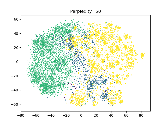
(a) cNV${{}_{sum}^{(en)}}\thinspace$; cNV${{}_{sum}^{(de)}}\thinspace$

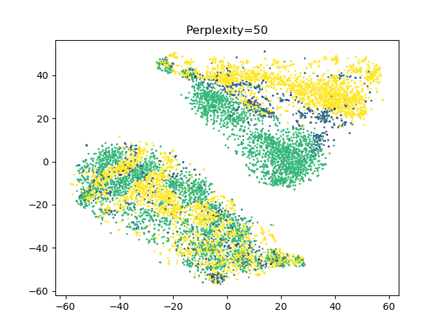
(b) NV${{}_{sum}^{(en)}}\thinspace$; NV${{}_{sum}^{(de)}}\thinspace$

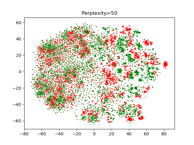
(c) cNV${{}_{sum}^{(en)}}\thinspace$; cNV${{}_{sum}^{(de)}}\thinspace$

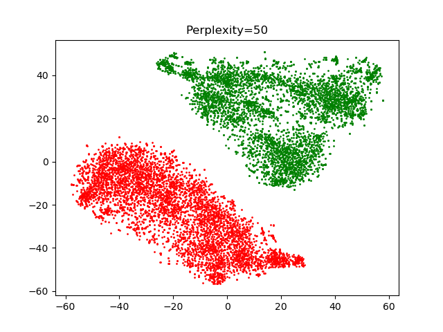
(d) NV${{}_{sum}^{(en)}}\thinspace$; NV${{}_{sum}^{(de)}}\thinspace$

Figure 2: The distribution of embeddings from the four document classes (subfigure a, b) and the distribution of English and German embeddings (subfigure c, d) in the test set.

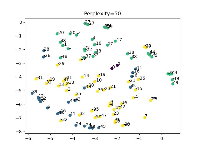
(a) cNV${{}_{sum}^{(en)}}\thinspace$; cNV${{}_{sum}^{(de)}}\thinspace$

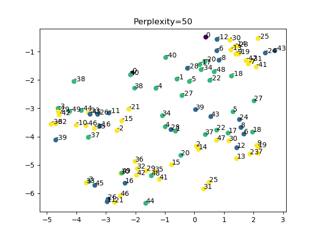
(b) NV${{}_{sum}^{(en)}}\thinspace$; NV${{}_{sum}^{(de)}}\thinspace$

Figure 3: English (+ve) and German (-ve) embedding pairs of 50 randomly sampled documents.

4 Results

Table 2: Classification accuracy (%) on CLDC

Method	en$\rightarrow$de	de$\rightarrow$en	Method	en$\rightarrow$de	de$\rightarrow$en
MTbs [10]	68.1	67.4	NV${{}_{sum}}\thinspace$[13] @	93.5	82.3
NMTbs	92.9	70.8	NV:  [13] @	94.4	82.7
$para\_doc$ [12]*	92.7	91.5	cNV${{}_{sum}^{(en)}}\thinspace$@	93.1	82.8
BAE [2]	91.8	74.2	cNV${{}_{sum}^{(de)}}\thinspace$@	93.2	81.4
ADD [1]	86.4	74.7	cNV${{}_{sum}}\thinspace$@	94.1	83.0
BI [1]	86.1	79.0	cNV${{}_{con}}\thinspace$@	94.3	83.3
BRAVE [3]	89.7	80.1	NV${{}_{sum}^{(y)}}\thinspace$	35.6	41.9
MultiVec [4]	88.2	79.1	cNV${{}_{sum}^{(y)}}\thinspace$	88.9	79.1
Unsup [24]	90.7	80.0	cNV${{}_{con}^{(y)}}\thinspace$	89.8	81.0

• cNV${{}_{\star}^{(en)}}\thinspace$(Fig. 1(b)) only goes through the en$\rightarrow$de path (if the input is German, it is first translated into English by NMT); similar for cNV${{}_{\star}^{(de)}}\thinspace$. cNV${{}_{\star}^{(y)}}\thinspace$(Fig. 1(c)) only goes through the en$\rightarrow$de path if the input is English, and only the de$\rightarrow$en path if the input is German; no translation is needed. On the other hand, cNV${{}_{\star}}\thinspace$(Fig. 1(d)) is the sum of cNV${{}_{\star}^{(en)}}\thinspace$and cNV${{}_{\star}^{(de)}}\thinspace$, so the translation is needed in computing one of them. NMT is trained with the same Europarl corpus. BAE adds monolingual test data in the training, whereas others do not.

Table 2 presents the performance of various embedding methods on the cross-lingual document classification task. They can be categorized into 3 types of methods: ‘*’ methods use iterative back-propagation(BP) optimization during the production of document vectors; ‘@’ methods use a forward pass of NMTs (trained with Europarl) to enhance performance (i.e., ‘NMT-assisted-forward’ methods); other results are trained with Europarl and only employ one-time forward pass of their respective model (i.e., forward method). MT_bs is the machine translation baseline from [10]. NMT_bs is the performance of the NMT model on which the cNV model was built. In NMT_bs, the classifier was trained with the term frequency/inverse document frequency of the most frequent 50000-word features. Among all the results, cNV${{}_{con}}\thinspace$is significantly better than $para\_doc$ ($p=0.000215$) in en$\rightarrow$de. For de$\rightarrow$en, our cNV${{}_{con}}\thinspace$gives the second-best result. It is also more convenient to use than methods (e.g., $para\_{doc}$) that require BP in production mode. As BP training is done iteratively and involving derivative calculations, it is not fit for situations that require fast online decoding. Moreover, the vectors produced by BP training will not be consistent in different runs or different systems (e.g., with different training epochs, random initialization, different batch sizes). Thus the forward pass method has a unique advantage in many applications.

The cNV model use either the ‘NMT-assisted-forward’ method or the ‘forward’ method. This flexibility is made possible because the embeddings produced by the cNV model from the same document in a language pair are very similar, and one may use either one of them or both for cross-lingual document classification. cNV${{}_{con}}\thinspace$shares similar good results with NV_:  ($p=0.022064$ in en$\rightarrow$de, $p=0.011092$ in de$\rightarrow$en). Among the ‘forward’ methods, cNV${{}_{con}^{(y)}}\thinspace$is not significantly worse than the ‘Unsup’ method ($p=0.143811$) in en$\rightarrow$de. cNV${{}_{con}^{(y)}}\thinspace$is significantly better than the ‘BRAVE’ method ($p=0.000169$) in de$\rightarrow$en. Therefore, cNV${{}_{con}}\thinspace$and cNV${{}_{con}^{(y)}}\thinspace$are among the best methods in ‘NMT-assisted-forward’ and ‘forward’ categories, respectively. The cNV${{}_{con}}\thinspace$result shows that using the NMT and producing document vectors together with cNV is better than using the NMT alone (NMT_bs). When we want to have the best performance, we can use the cNV${{}_{con}}\thinspace$model. On the other hand, when we want a lighter model and faster decoding, we can use cNV${{}_{con}^{(y)}}\thinspace$without the NMT. Note that we do not need to change the model structure, nor do we need to retrain the cNV model when shifting from cNV${{}_{con}}\thinspace$to cNV${{}_{con}^{(y)}}\thinspace$; the only difference between these two modes is whether we plug in the translated result from NMT into the other encoder. On the other hand, NV model must use the embedding from the same language (or the combination of two embeddings) in training and testing (please see Fig. 1) and all good NV results belong to the ‘NMT-assisted-forward’ methods. We further verify the poor performance of NV${{}_{\star}^{(y)}}\thinspace$as shown in Table 2.

Without the distance constraint, the English embedding and its corresponding German embedding of the same document is not guaranteed to lie in the same vector space and cannot be compared. To further illustrate this, we visualize the document embeddings of different languages using their t-SNE projections in Fig. 2 and 3. Fig. 2 shows the NV/cNV embeddings of German documents in the ${en\rightarrow de}$ test set. We also translate the same documents into a mirrored English set with the NMT to show the distribution of the same documents in a different language. In Fig. 2 (a) and (b), the 4 types of documents are plotted in 4 different colors (red: Corporate/Industrial, blue: Economics, green: Government/Social, yellow: Market). The document embeddings are clearly divided into 4 clusters, but only when they are trained with distance constraint then their German embeddings and English embeddings (from the translation of the German texts) are indistinguishable if they belong to the same type. On the other hand, in Fig. 2 (c) and (d), English embeddings are shown in red while their German counterparts of the same documents are shown in green regardless of their document types. It is clear that without the distance constraint training, the NV document embeddings are segregated by the languages into two major clusters. These figures show that simply sharing layers in the NV model without distance constraint training is not sufficient to produce similar embeddings from two languages and they cannot be compared.

Fig. 3 shows the t-SNE projections of 50 English-German document embedding pairs. The positive and negative indices refer to the English and German embeddings produced from the same indexed document in the German test set, respectively. For example, ‘-2’ is the German embedding of the 2nd document in the test set, whereas ‘2’ is the English embedding of the same 2nd German document after it is translated to English. It shows that cNV model, trained with the distance constraint, effectively pairs the German and English embeddings from two parts of the model close together, regardless of their different encoders and language inputs. On the other hand, the English and German NV embeddings of the same document are far apart. This also explains why the previous NV model must use an NMT as a bridge to achieve good classification performance, and why in the current cNV model the NMT is not necessary.

5 Conclusion

Compared with the previous NV model where the embeddings are segregated across different languages, cNV embedding pairs are very close to each other. This opens future research directions in the fast conversion of the existing NMT models to cross-lingual text embedding models.

References

- [1] K. M. Hermann and P. Blunsom, “Multilingual models for compositional distributional semantics,” in Proceedings of ACL, 2014.
- [2] S. C. AP, S. Lauly, H. Larochelle, M. Khapra, B. Ravindran, V. C. Raykar, and A. Saha, “An autoencoder approach to learning bilingual word representations,” in Advances in Neural Information Processing Systems, 2014, pp. 1853–1861.
- [3] A. Mogadala and A. Rettinger, “Bilingual word embeddings from parallel and non-parallel corpora for cross-language text classification,” in Proceedings of the 2016 Conference of the North American Chapter of the Association for Computational Linguistics: Human Language Technologies, 2016, pp. 692–702.
- [4] A. Bérard, C. Servan, O. Pietquin, and L. Besacier, “Multivec: a multilingual and multilevel representation learning toolkit for NLP,” in The 10th edition of the Language Resources and Evaluation Conference (LREC), 2016.
- [5] D. C. Ferreira, A. F. Martins, and M. S. Almeida, “Jointly learning to embed and predict with multiple languages,” in Proceedings of the 54th Annual Meeting of the Association for Computational Linguistics (Volume 1: Long Papers), vol. 1, 2016, pp. 2019–2028.
- [6] S. Gouws, Y. Bengio, and G. Corrado, “Bilbowa: Fast bilingual distributed representations without word alignments,” in International Conference on Machine Learning, 2015, pp. 748–756.
- [7] M. Artetxe and H. Schwenk, “Margin-based parallel corpus mining with multilingual sentence embeddings,” arXiv preprint arXiv:1811.01136, 2018.
- [8] H. Schwenk and X. Li, “A corpus for multilingual document classification in eight languages,” arXiv preprint arXiv:1805.09821, 2018.
- [9] R. A. Sinoara, J. Camacho-Collados, R. G. Rossi, R. Navigli, and S. O. Rezende, “Knowledge-enhanced document embeddings for text classification,” Knowledge-Based Systems, vol. 163, pp. 955–971, 2019.
- [10] A. Klementiev, I. Titov, and B. Bhattarai, “Inducing crosslingual distributed representations of words,” Proceedings of COLING 2012, pp. 1459–1474, 2012.
- [11] J. Coulmance, J.-M. Marty, G. Wenzek, and A. Benhalloum, “Trans-gram, fast cross-lingual word-embeddings,” in Proceedings of the 2015 Conference on Empirical Methods in Natural Language Processing, 2015, pp. 1109–1113.
- [12] H. Pham, T. Luong, and C. Manning, “Learning distributed representations for multilingual text sequences,” in Proceedings of the 1st Workshop on Vector Space Modeling for Natural Language Processing, 2015, pp. 88–94.
- [13] W. Li and B. Mak, “Fast derivation of cross-lingual document vectors from self-attentive neural machine translation model,” in Proceedings of Interspeech, Hyderabad, India, September 2018, pp. 107–111.
- [14] D. D. Lewis, Y. Yang, T. G. Rose, and F. Li, “Rcv1: A new benchmark collection for text categorization research,” Journal of machine learning research, vol. 5, no. Apr, pp. 361–397, 2004.
- [15] Z. Yang, Z. Dai, Y. Yang, J. Carbonell, R. R. Salakhutdinov, and Q. V. Le, “Xlnet: Generalized autoregressive pretraining for language understanding,” in Advances in neural information processing systems, 2019, pp. 5754–5764.
- [16] H. Schwenk and M. Douze, “Learning joint multilingual sentence representations with neural machine translation,” arXiv preprint arXiv:1704.04154, 2017.
- [17] M. Artetxe and H. Schwenk, “Massively multilingual sentence embeddings for zero-shot cross-lingual transfer and beyond,” Transactions of the Association for Computational Linguistics, vol. 7, pp. 597–610, 2019.
- [18] D. S. Sachan and G. Neubig, “Parameter sharing methods for multilingual self-attentional translation models,” arXiv preprint arXiv:1809.00252, 2018.
- [19] R. Sennrich, O. Firat, K. Cho, A. Birch, B. Haddow, J. Hitschler, M. Junczys-Dowmunt, S. Läubli, A. V. Miceli Barone, J. Mokry, and M. Nadejde, “Nematus: a toolkit for neural machine translation,” in Proceedings of the Software Demonstrations of the 15th Conference of the European Chapter of the Association for Computational Linguistics. Valencia, Spain: Association for Computational Linguistics, April 2017, pp. 65–68. [Online]. Available: http://aclweb.org/anthology/E17-3017
- [20] Z. Tu, Y. Liu, Z. Lu, X. Liu, and H. Li, “Context gates for neural machine translation,” Transactions of the Association of Computational Linguistics, vol. 5, no. 1, pp. 87–99, 2017.
- [21] Y. Ding, Y. Liu, H. Luan, and M. Sun, “Visualizing and understanding neural machine translation,” in Proceedings of the 55th Annual Meeting of the Association for Computational Linguistics (Volume 1: Long Papers), vol. 1, 2017, pp. 1150–1159.
- [22] A. Vaswani, N. Shazeer, N. Parmar, J. Uszkoreit, L. Jones, A. N. Gomez, L. Kaiser, and I. Polosukhin, “Attention is all you need,” in Advances in Neural Information Processing Systems, 2017, pp. 6000–6010.
- [23] P. Koehn, “Europarl: A parallel corpus for statistical machine translation,” in MT summit, vol. 5, 2005, pp. 79–86.
- [24] T. Luong, H. Pham, and C. D. Manning, “Bilingual word representations with monolingual quality in mind,” in Proceedings of the 1st Workshop on Vector Space Modeling for Natural Language Processing, 2015, pp. 151–159.