MISS: Finding Optimal Sample Sizes for Approximate Analytics

Nowadays, sampling-based Approximate Query Processing (AQP) is widely regarded as a promising way to achieve interactivity in big data analytics. To build such an AQP system, finding the minimal sample size for a query regarding given error constraints in general, called Sample Size Optimization (SSO), is an essential yet unsolved problem. Ideally, the goal of solving the SSO problem is to achieve statistical accuracy, computational efficiency and broad applicability all at the same time. Existing approaches either make idealistic assumptions on the statistical properties of the query, or completely disregard them. This may result in overemphasizing only one of the three goals while neglect the others.

To overcome these limitations, we first examine carefully the statistical properties shared by common analytical queries. Then, based on the properties, we propose a linear model describing the relationship between sample sizes and the approximation errors of a query, which is called the error model. Then, we propose a Model-guided Iterative Sample Selection (MISS) framework to solve the SSO problem generally. Afterwards, based on the MISS framework, we propose a concrete algorithm, called $L^{2}$Miss, to find optimal sample sizes under the $L^{2}$ norm error metric. Moreover, we extend the $L^{2}$Miss algorithm to handle other error metrics. Finally, we show theoretically and empirically that the $L^{2}$Miss algorithm and its extensions achieve satisfactory accuracy and efficiency for a considerably wide range of analytical queries.

1 Introduction

In the Big Data era, analyzing large volumes of data by analytical queries, which summarize the data to discover useful information, becomes extremely challenging for data scientists. This is mainly because under such circumstance, it is infeasible to check the data record-by-record manually. Therefore, people are always hoping to design systems to fully automate this process. However, none of these efforts perfectly solves this problem. Therefore, recent years have witnessed a surge of interest in designing novel systems to interact with humans. By leveraging human knowledge, far more insights can be obtained from the data with analytical queries.

However, the goal of incorporating human intelligence in analytical queries brings new challenges. One of them that is the most essential yet elusive is interactivity [28]. To cope with it, one of the most effective approach is to reduce the amount of data to be processed by sampling, which is called sampling-based Approximate Query Processing (AQP) [28]. The use cases for sampling-based AQP typically include helping users to obtain a quick understanding of the data. Such understanding may be inaccurate, but can be of great help for later complicated and mission-critical analytical tasks.

When running an approximate analytical query, users would like to ensure that the approximate result and the true one is almost the same. The difference between these two results is called the approximation error, which is measured by an error metric chosen according to different scenarios, such as the $L^{2}$ norm. To lower query latency and achieve interactivity for the query, we hope to reduce the size of the sample to be processed by a given query as much as possible. Therefore, one of the key problem in sampling-based AQP is Sample Size Optimization (SSO), i.e., to find the minimal sample size required to answer an approximate query while ensuring that the approximation error satisfies given constraints.

Challenges: When we consider solving the SSO problem, several challenges arise due to its inherent uncertainty introduced by sampling. More specifically, it is far from trivial to achieve all of the following goals.

• Statistical accuracy, which means that the resulting sample size is large enough to ensure that the approximate query result satisfies the user-defined error constraints. To ensure accuracy, error estimation methods are required to test whether the constraints hold. However, these methods often make strong assumptions on the query, which limit their range of application.

• Computational efficiency, which means not only that the sample size should be as small as possible to maximize the speed of analytical queries, but also that SSO algorithms themselves should be efficient enough to avoid hampering the performance of the whole analytical process. To improve efficiency, the sample size should be as small as possible, which may increase the risk of being inaccurate.

• Broad applicability, which means that the assumptions on both the data and the analytical functions should be weak enough to accommodate a wide variety of analytical tasks. To broaden the range of applications, error estimation methods based on weak assumptions are in demand. However, although adopting these methods might be beneficial in terms of applicability, it is often at the cost of efficiency since these methods are typically computationally intensive [39].

Limitations of existing methods: From the discussions above, the three goals of solving the SSO problem may contradict with each other. Thus, achieving all of them at the same time seems impossible. Existing SSO methods often fall short in one or more of the three aspects above. Specifically,

• Statistical accuracy: To estimate the approximation error, some methods [3, 33, 25] assume that the sampling distribution is approximately normal such that the standard interval [12] could be applied. However, such assumptions do not always hold, which brings the risk of producing inaccurate results. What’s worse, this happens rather frequently [2].

• Computational efficiency: Some methods [23, 13, 4] rely on concentration inequalities [10] such as Hoeffding’s inequality [19] for error estimation. Such estimation is so conservative that it requires much larger sample size than necessary to meet the constraints [2], making it inefficient in terms of sample size. Some other methods [38] find optimal sample sizes in a mini-batch approach, which may result in a huge number of trials before the constraints are met and is inefficient in terms of the running time of the SSO method itself.

• Broad applicability: Methods that exploit normality and concentration inequalities require assumptions on the analytical function to guarantee accuracy for a query. For example, the central limit theorem (CLT) [8] only works when the analytical function is AVG. This makes it hard to apply the SSO methods to arbitrarily complex analytical functions.

In summary, most existing methods overemphasize only one of the three goals while paying little attention to the others by either making idealistic assumptions on the statistical properties of the approximate analytical query or almost completely ignoring them.

Our contributions: Being aware of the limitations, by using a novel parametric model based on reasonably weak assumptions, we design a family of different novel SSO methods under the same proposed framework but suitable for various error metrics. The methods based on our framework not only have maximum applicability being able to support almost all kinds of analytical queries, but also achieve a decent balance between accuracy and efficiency by selecting samples as small as possible while ensuring the error constraints to be satisfied.

• To maximize applicability, we propose a Model-guided Iterative Sample Selection (MISS) framework for generally addressing the SSO problem. It allow users to customize error metrics, sampling methods and error estimation methods for different scenarios and makes no assumption on the data and the query.

• To balance accuracy and efficiency, we propose a linear error model describing the relationship between approximate errors and the sample sizes. Then, by combining the MISS framework and the error model, we propose an algorithm called $L^{2}$Miss that finds the optimal sample size for $L^{2}$ norm error. We show theoretically and empirically that $L^{2}$Miss is efficient while being accurate.

• To cope with different error metrics, we extend the $L^{2}$Miss algorithm under the MISS framework by converting the error constraints defined in terms of $L^{2}$ norm error to other metrics. Both theoretical and empirical study show that the extensions can handle a large variety of data and analytical functions efficiently, while providing satisfactory accuracy.

Organization: In Section 2, we define the SSO problem formally and develop the error model. In Section 3, we propose MISS, a general framework for solving the SSO problem. In Section 4 and Section 5, we develop a series of algorithms under the MISS framework to solve the SSO problem under various error metrics. Experimental evaluation is presented in Section 6, followed by related work in Section 7. We state our conclusion and discuss future work in Section 8.

2 Preliminaries

2.1 Problem Description

In this paper, we mainly focus on analytical queries, which obtain summaries from data. Following the convention in BlinkDB [3], we define approximate analytical queries as LABEL:lst:query.

Listing 1: Approximate Analytical Queries

⬇

SELECT $X,f(Y)$ FROM $D(X,Y)$

GROUP BY $X$ WHERE $P$

ERROR WITHIN $\epsilon$ CONFIDENCE $1-\delta$

Here, $D$ denotes the dataset to perform the query on. $X$ and $Y$ are two sets of attributes in $D$. Following the convention in OLAP [17], we call the attribute set $X$ the group-by attributes, or dimensions; and $Y$ the analytical attributes, or measures. $P$ denotes the selection predicate, which is intended for the COUNT-with-predicate queries. $f$ is called the analytical function computing the analytical results over $Y$ grouped by $X$.

We denote the true analytical result on $D$ and its approximation as $\boldsymbol{\mathbf{\theta}}$ and $\boldsymbol{\mathbf{\hat{\theta}}}$ respectively. Note that for a $m$-group query, $\boldsymbol{\mathbf{\theta}}$ and $\boldsymbol{\mathbf{\hat{\theta}}}$ are both $m$-dimensional vectors, each of which the entry corresponds to the query result of one group. To measure the approximation error, we denote $d$ as the error metric, and the error can be expressed as $d{}\left(\boldsymbol{\mathbf{\hat{\theta}}},\boldsymbol{\mathbf{\theta}}\right)$. To bound the error, we define error constraints to have the form of

$$\operatorname{Pr}\left\{d{}\left(\boldsymbol{\mathbf{\hat{\theta}}},\boldsymbol{\mathbf{\theta}}\right)\leq\epsilon\right\}\geq 1-\delta,$$ (1)

where $\epsilon$ is called the error bound, $\delta$ is called the error probability, and $1-\delta$ is called the confidence. From a statistical point of view, Equation 1 states that the margin of error [27] of $\boldsymbol{\mathbf{\hat{\theta}}}$ is no greater than $\epsilon$ with confidence $1-\delta$.

Note that throughout the paper, we assume that all the data are stored in a single table. We refer readers to [26] for the approximate processing techniques of joins. We also would not consider handling selections in a general circumstances other than COUNT-with-predicate queries. For AQP of selections, we recommend readers to refer to [13] for more discussion.

In order to answer a query like in LABEL:lst:query approximately, we draw a sample $S\subseteq D$ from the dataset $D$, and apply the analytical function $f$ on $S$ to obtain the approximate result. For an $m$-group query, we denote the size of each group in $S$ and $D$ as $n_{i}$ and $|D|_{i}$, respectively, where $i=1,2,\ldots,m$. For convenience, we use $\boldsymbol{\mathbf{n}}$ to denote the vector of sample size, i.e., $\boldsymbol{\mathbf{n}}=\begin{pmatrix}n_{1}&n_{2}&\cdots&n_{m}\end{pmatrix}^{\mathsf{T}}$. To find optimal samples, we attempt to minimize the total sample size, which is defined as the sum of sample sizes of all groups, i.e.,

$$C\left(\boldsymbol{\mathbf{n}}\right)=\sum_{i=1}^{m}n_{i}=\boldsymbol{\mathbf{1}}^{\mathsf{T}}\boldsymbol{\mathbf{n}}.$$ (2)

Using the concept of error metric and total sample size, the SSO problem, which aims to find the optimal sample size subject to the predefined error constraint, is formalized as follows.

Definition 1.

Given an approximate analytical query in LABEL:lst:query, the sample size optimization problem is to

$$\min_{\boldsymbol{\mathbf{n}}}C(\boldsymbol{\mathbf{n}})\quad s.t.\quad\operatorname{Pr}\left\{d{}\left(\boldsymbol{\mathbf{\hat{\theta}}},\boldsymbol{\mathbf{\theta}}\right)\leq\epsilon\right\}\geq 1-\delta$$ (3)

where $\boldsymbol{\mathbf{n}}$ is the size of the sample $S$ drawn from $D$, $\epsilon$ denotes the error bound and $\delta$ denotes the error probability.

Solving the problem in Definition 1 is far from trivial. This is because (i) the approximation error $d{}\left(\boldsymbol{\mathbf{\hat{\theta}}},\boldsymbol{\mathbf{\theta}}\right)$ is random, which makes the problem stochastic rather than deterministic; and (ii) the closed-form expression of $d{}\left(\boldsymbol{\mathbf{\hat{\theta}}},\boldsymbol{\mathbf{\theta}}\right)$ is unknown. The two reasons make it impossible to apply the conventional optimization algorithms such as gradient-based ones to find the optimum [5]. One effective way of alleviating the two issues together is to approximate $d{}\left(\boldsymbol{\mathbf{\hat{\theta}}},\boldsymbol{\mathbf{\theta}}\right)$ with a surrogate model [7], which we call the error model to reduce the impact of noise and to guide the process of finding the optimal sample size.

2.2 Modeling Approximation Errors

Next, we would like to develop the error model, which takes a sample size $\boldsymbol{\mathbf{n}}$ as the input and outputs the predicted approximation error using samples of size $\boldsymbol{\mathbf{n}}$ to approximately answer the query.

2.2.1 Statistical Properties of Analytical Queries

To derive the model, we first examine the asymptotic properties shared by common analytical queries, i.e., how approximation errors decrease as sample sizes increase for typical queries. We then derive the error model based on such properties.

In order to simplify the discussions, we assume that, queries only involve a single group and denote the sample size, the true and the approximate analytical result by $n$, $\theta$ and $\hat{\theta}$ respectively. Later, we will extend the discussion to the multi-group case for completeness in this section.

Relationship between error and sample size. Intuitively, approximation errors decrease as the corresponding sample sizes increase. To formalize the intuition, We employ the concept of convergence in probability theory and quantify how the error decreases using its rate of convergence in probability [32], which is defined as follows.

Definition 2.

Given the approximation error $d\left(\hat{\theta},\theta\right)$ that converges in probability, the rate of convergence in probability of $d\left(\hat{\theta},\theta\right)$ is $O(r_{n})$ if $r_{n}^{-1}d\left(\hat{\theta},\theta\right)=O_{p}(1)$, where $O_{p}(1)$ means “bounded in probability”.

Intuitively, the $O_{p}$ notation shares the same idea with the $O$ notation in computational complexity in that for any two sequence $\left\{a_{n}\right\}$ and $\left\{b_{n}\right\}$, $a_{n}=O\left(b_{n}\right)$ if and only if the ratio $a_{n}/b_{n}$ is bounded by a constant for a sufficiently large $n$, while $a_{n}=O_{p}\left(b_{n}\right)$ means that the ratio $a_{n}/b_{n}$ is bounded with arbitrarily large probability. Note that for convenience, we omit the term “in probability” when talking about convergence unless otherwise specified in the rest of this paper.

Analytical results as statistics. To find the the rate of convergence of error for different types of queries using statistical theory, we claim that for a sample $S=\left\{X_{1},X_{2},\ldots,X_{n}\right\}$, the results of a large variety of analytical queries can be classified in to at least one of the following three types of statistics:

• U-statistics [18], which is of the form

  $$U_{n}=\binom{n}{k}^{-1}\sum_{\nu}\kappa\left(X_{\nu_{1}},X_{\nu_{2}},\ldots,X_{\nu_{k}}\right),$$ (4)

  where $\left\{\nu_{1},\nu_{2},\ldots,\nu_{k}\right\}$ is a subset of $\left\{1,2,\ldots,n\right\}$. Examples of U-statistics include common aggregate functions, e.g., AVG, VARIANCE, and PROPORTION [32].

• M-estiamtors [20], which is of the form

  $$M_{n}=\operatorname*{arg\,max}_{\theta}\sum_{i=1}^{n}\psi_{\theta}\left(X_{i}\right),$$ (5)

  where $\theta$ is the parameter to be estimated, and $\psi_{\theta}$ are known functions. Examples of M-estimators include typical machine learning methods, such as linear regression, logistic regression and kernel regression [32].

• Inconsistent estimators, of which the approximation errors do not converge to zero in probability, such that the error would not keep on decreasing with the increase of sample sizes. Examples of inconsistent estimators include some aggregate functions, such as SUM and COUNT [32].

Rate of convergence of common statistics. To derive the error model, we examine the rate of convergence for common statistics, including the three categories above and others.

• The rate of convergence of U-statistics and M-estimators is given by the following lemma.

  Lemma 1

  Under weak conditions [32], the rate of convergence of U-statsitics $U_{n}$ and M-estimators $M_{n}$ are both $O\left(n^{-b}\right)$, where $b$ is a positive constant.

• For inconsistent estimators, it may be impossible to find the optimal sample size directly since the approximation errors may not continue to decrease no matter how the sample sizes increase. Fortunately, for some queries in this category, there exists a transformation converting them to consistent estimators, such as U-statistics and M-estimators. For example,

  $$\texttt{SUM}\left(Y\right)=|D|\cdot\texttt{AVG}\left(Y\right),\quad\texttt{COUNT}\left(Y\right)=|D|\cdot\texttt{PROPORTION}\left(Y\right)$$

  where $|D|$ denotes the size of $D$. In such case, we can express the error constraints with respect to the corresponding consistent estimators using the transformation, and then optimize the sample size subject to the transformed constraints. And the actual error can be obtained by applying the inverse transformation.

• For some other statistics such as QUANTILE that are not U-statistics or M-estimators, they may be transformed into the two categories. Under specific conditions, these statistics may also converge at rate $O\left(n^{-b}\right)$. Therefore, we claim that the convergence rate of many types of statistics, besides U-statistics and M-estimators, also has the form of $O\left(n^{-b}\right)$.

Observation. To summarize, we observe that, even though the concrete expressions of analytical queries may differ, many of them still share one principal asymptotic property, which is stated as the following proposition.

Proposition 2

For common analytical queries, the approximation error $d\left(\hat{\theta},\theta\right)$ converges at rate $O\left(n^{-b}\right)$.

2.2.2 The Error Model

Based on the observation above, we derive the error model to approximate the relationship between sample sizes and errors.

Single-group error model. We first consider the single-group case. According to Proposition 2, $d\left(\hat{\theta},\theta\right)=O_{P}\left(n^{-b}\right)$. Observe that in real-world applications, the absolute size of samples, i.e., $n$ is typically large. Therefore, it is reasonable to ignore the lower-order terms in the $O_{P}$ notation and only use the leading term. Therefore, the single-group error is

$$d\left(\hat{\theta},\theta\right)\approx an^{-b}$$ (6)

where $a$, $b$ are constants. The logarithm of right hand side is called the single-group error model, which is linear to $n$.

Multi-group error model. To derive the multi-group error model, we first consider a specific error metric $d_{g}$, which is defined as the geometric mean of the errors of all groups. Specifically, by plugging Equation 6 into the equation above, we have

$$d{{}_{g}}\left(\boldsymbol{\mathbf{\hat{\theta}}},\boldsymbol{\mathbf{\theta}}\right)=\sqrt[m]{\prod_{i=1}^{m}{d\left(\hat{\theta}_{i},\theta_{i}\right)}}==\sqrt[m]{\prod_{i=1}^{m}{a_{i}n_{i}^{-b_{i}}}}$$

where $d\left(\hat{\theta}_{i},\theta_{i}\right)$ is the error of group $i$, and $a_{i}$, $b_{i}$ are all constants. Logarithms are then token on both side gives

$$\log d{{}_{g}}\left(\boldsymbol{\mathbf{\hat{\theta}}},\boldsymbol{\mathbf{\theta}}\right)=\frac{1}{m}\left(\sum_{i=1}^{m}\log a_{i}-{\sum_{i=1}^{m}{b_{i}n_{i}}}\right)=\beta_{0}-\sum_{i=1}^{m}\beta_{i}\log n_{i},$$

where $\beta_{i}$ are all constants.

The right hand side of the second equation above, which is denoted by $H\left(\boldsymbol{\mathbf{n}};\boldsymbol{\mathbf{\beta}}\right)$, is called the multi-group error model, or simply the error model, where $\boldsymbol{\mathbf{\beta}}=\begin{pmatrix}\beta_{0}&\beta_{1}&\cdots&\beta_{m}\end{pmatrix}^{\mathsf{T}}$ is the parameter vector. For convenience, we denote $\tilde{\boldsymbol{\mathbf{n}}}=\begin{pmatrix}1&-\log n_{1}&-\log n_{2}&\cdots&-\log n_{m}\end{pmatrix}^{\mathsf{T}}$. The model is then rewritten as

$$H\left(\boldsymbol{\mathbf{n}};\boldsymbol{\mathbf{\beta}}\right)=\boldsymbol{\mathbf{\beta}}^{\mathsf{T}}\tilde{\boldsymbol{\mathbf{n}}},$$

which is linear. Moreover, we use the notation $H\left(\boldsymbol{\mathbf{n}};\boldsymbol{\mathbf{\hat{\beta}}}^{(k)}\right)$ to denote the model with parameter $\boldsymbol{\mathbf{\beta}}=\boldsymbol{\mathbf{\hat{\beta}}}^{(k)}$ and $H\left(\boldsymbol{\mathbf{n}}^{(k)};\boldsymbol{\mathbf{\hat{\beta}}}^{(k)}\right)$ to denote the value of the model with parameter $\boldsymbol{\mathbf{\beta}}=\boldsymbol{\mathbf{\hat{\beta}}}^{(k)}$ at sample size $\boldsymbol{\mathbf{n}}=\boldsymbol{\mathbf{n}}^{(k)}$. We use $\boldsymbol{\mathbf{\hat{\beta}}}$ to denote the estimated value of $\boldsymbol{\mathbf{\beta}}$.

Even though the error model $H\left(\boldsymbol{\mathbf{n}};\boldsymbol{\mathbf{\beta}}\right)$ is defined assuming that the error metric is the geometric mean, as we will show in Section 4 and Section 5, it performs well for other commonly-used error metrics.

3 Framework

In this section, we propose the MISS framework to solve the SSO problem with as few assumptions as possible. Specifically, we make no assumption on the data, the query, the error metric, the sampling and the error estimation methods. By doing so, we provide users a general enough approach to solve the problem.

Since the SSO problem involves black-box functions as constraints, finding an exact closed-form solution is hard in general. Therefore, existing AQP systems try to find an approximate solution using one of the following two approaches, as discussed in Section 1.

• The formula-based approach ideally assumes that a closed-form approximation equation in terms of the sample size and the error is known. The predicted sample size can be directly obtained by solving the equation with respect to the desired error constraint [2].

• The model-free approach exploits no priori knowledge of the relationship between sample size and approximation error, and simply guess the optimum by increasing the sample size by a small step in each iteration until the error constraint is satisfied [38]. The process of generating the guess in each iteration is call sample size searching.

The formula-based approach is usually efficient enough by simply solving a closed-form equation while the model-free approach is able to provide sufficient accuracy guarantees and broadly applicable for a variety of queries by making only a few assumptions. However, both approaches fail to balance accuracy, efficiency and applicability. The former might suffer from inaccuracy or limited applicability due to its idealistic assumptions, while the latter might suffer from inefficiency due to the ignorance of the statistical property.

To make the best of their advantages while overcome their disadvantages, we propose the Model-guided Iterative Sample Selection (MISS) framework to solve the SSO problem generally. MISS iteratively estimates the error with respect to the predicted sample size, polishes the model according to the of sample sizes and errors observed, and makes the prediction again.

This approach has two advantages. On one hand, by using a flexible model rather than a fixed equation and iterative prediction, the risk of obtaining inaccurate sample size can be greatly reduced compared to the formula-based approach. On the other hand, this framework takes the advantage of the error model introduced in Section 2.2 to predict the optimal sample size such that the unnecessary searching can be largely avoid compared to the model-free approach.

The basic idea of our MISS framework is to start with an initial guess of the sample size, then to iteratively search for the optimum until the error constraint is satisfied.

Input: Dataset $D$, analytical function $f$, error bound $\epsilon$ with error probability $\delta$, and error metric $d$.

Output: Sample $S\subsetneqq D$ such that the approximation error $d{{}_{L^{2}}}\left(\boldsymbol{\mathbf{\hat{\theta}}},\boldsymbol{\mathbf{\theta}}\right)\leq\epsilon$ with probability $1-\delta$.

1 $P\leftarrow\emptyset$

2 $\boldsymbol{\mathbf{n}}\leftarrow\operatorname{\textsc{Initialize}}\left(\right)$

3 while True do

4      $S\leftarrow\operatorname{\textsc{Sample}}\left(D,\boldsymbol{\mathbf{n}}\right)$

5       $e\leftarrow\operatorname{\textsc{Estimate}}\left(S,d,f,\delta\right)$

6       if $e\leq\epsilon$ then return $S$

7       else

8            $P\leftarrow P\cup\left\{\left(\boldsymbol{\mathbf{n}},e\right)\right\}$

9             $\boldsymbol{\mathbf{n}}\leftarrow\operatorname{\textsc{Predict}}\left(P,\epsilon\right)$

Algorithm 1 The MISS Framework

The details of the MISS framework in shown in Algorithm 1. The MISS framework first generates an initial guess of the sample size in Line 1. Then in each iteration, the framework draws a sample of the generated size in Line 1. Next, it estimates the approximation error in terms of the sample in Line 1. Afterwards, it tests whether the error constraint is satisfied in Line 1. If the constraint is satisfied, it returns the selected sample of optimal size successfully. Otherwise, in Line 1, the estimated error and the sample size is collected as the error profile defined as

$$P=\left\{\left(\boldsymbol{\mathbf{n}}^{(j)},e^{(j)}\right)\middle|1\leq j\leq k\right\}$$ (7)

for prediction, where $l$ is the number of iterations. Within error profile, $\boldsymbol{\mathbf{n}}^{(j)}$ denotes the size of the sample in iteration $j$, and $e^{(j)}$ denotes the approximation error estimated in iteration $j$. Finally, it generates the predicted optimal sample size using the error model in Line 1. With testing mechanism, this framework ensures to terminate with the constraints satisfied.

The MISS framework is general enough to allow users to design the subroutines to meet their needs, i.e., the Initialize, Sample, Estimate, and Predict subroutines. The interfaces and functionalities of these subroutines are defined as follows.

• Initialize: it generates an initial guess of the sample size. For a better prediction, the initial guess typically should better be a sequence of sample sizes rather than a single value. The goal of determining initial guesses is to make predictions more accurate and reliable without compromising much of efficiency.

• Sample: it takes a sample $S$ randomly from the original dataset $D$ of size $\boldsymbol{\mathbf{n}}$.

• Estimate: it estimates the error $e$ of the approximate result with error probability $\delta$ in terms of the analytical function $f$ evaluated on the sample $S$ measured by the error metric $d$. Typically, relaxing the assumptions required by error estimation methods helps to enlarge the range of applications of the SSO algorithm.

• Predict: it predicts the optimal sample size $\boldsymbol{\mathbf{n}}$ using the error model. It uses the error profile $P$ to fit the model, then apply the model to find the optimum in terms of the total sample size $C$ subject to the error constraint. Specific models only work for specific categories of data, analytical functions and error metrics. When the model fails, the Predict subroutine recognizes the failure and returns an error.

According to the statistical properties and the performance requirements of the query to be processed, data analysts are able to develop specific SSO algorithms fit for their needs based on the MISS framework. As we will show in Section 4, for a specific scenario, by implementing the subroutines, a concrete SSO algorithm can be derived specifically. Moreover, as shown in Section 5, by extending the algorithm, we proposed a family of algorithms that work under various error metrics.

4 Finding Optimal Sample Sizes

In this section, we propose a concrete SSO algorithm for the $L^{2}$ norm error metric $d_{L^{2}}$, called $L^{2}$Miss, based on the MISS framework proposed in Section 3 and utilizing the error model described in Section 2.2. The $L^{2}$ norm error $d{{}_{L^{2}}}\left(\boldsymbol{\mathbf{\hat{\theta}}},\boldsymbol{\mathbf{\theta}}\right)$ is defined as the $L^{2}$ norm of approximation errors of all groups. Specifically,

$$d{{}_{L^{2}}}\left(\boldsymbol{\mathbf{\hat{\theta}}},\boldsymbol{\mathbf{\theta}}\right)=\sqrt{\sum_{i=1}^{m}{\left({\hat{\theta}}_{i}-{\theta}_{i}\right)}^{2}}$$ (8)

Under the MISS framework, the $L^{2}$Miss algorithm is developed by implementing the subroutines declared in Section 3. To illustrate the $L^{2}$Miss algorithm, we first introduce the sampling and the error estimation methods in order. Then, we show how to predict the optimal sample size in a model-guided approach. Finally, we present how to initialize the error profile to make better predictions without compromising much of efficiency.

4.1 Sampling

For sampling, To reduce the total sample size especially when the data size differs substantially for each group [29], we use uniform stratified sampling, which takes a sample of size $n_{i}$ from each group in $D$ uniformly at random. By controlling the sample size of each group individually, the total size of samples can be largely reduced.

To obtain a stratified sample, almost all existing data management platforms, such as Apache Spark [37], require a full scan. This is for two reasons. On one hand, the random sampling method offered by them is typically Bernoulli sampling [15], which assigns a probability to each record to determine whether it should be included in the sample. On the other hand, the GROUP BY clause requires to examine the group-by attributes for each record to determine which group it belongs to. However, full scans can be rather expensive when the data size is large.

Fortunately, we are able to avoid full scans in sampling by adopting two techniques: first, we use gap sampling [14], which assigns a probability only to the records in the sample instead of to all records; then, we use inverted index [34] on group-by attributes to avoid full scans to examine group membership. Specifically, we perform sampling on each inverted list for each combination of values of the group-by attributes and obtain the stratified sample using the index.

4.2 Error Estimation

For maximum applicability, we choose the bootstrap [12] for estimation. It does not make any assumption on the specific distribution of the data $D$ or the specific analytical function $f$, while only requires some weak regularity conditions to work as expected.

The bootstrap operates as follows [36]: to estimate the error of a statistic $T$ computed by the analytical function $f$, it draws $B$ resamples $S^{*}_{b}$, $b=1,2,\ldots,m$, from the original sample $S$ with replacement, each of the same size as $S$. For each resample, compute the estimate $T^{*}_{b}$ on $S^{*}_{b}$ in the same way as computing $T$ on $S$. Then it approximates the true sampling distribution of $T$, i.e., $F\left(t\right)=\operatorname{Pr}\left\{T\leq t\right\}$ by empirical distribution $\mathbb{F}\left(t\right)=\left(1/B\right)\sum_{b=1}^{B}\operatorname{I}\left\{T^{*}_{b}\leq t\right\}$, where $\operatorname{I}$ denotes the indicator random variable. The $1-\delta$ confidence region can be obtained by taking the $1-\delta$ quantile of $\mathbb{F}\left(t\right)$.

The correctness of the bootstrap depends on the consistency of approximating the true distribution $F\left(t\right)$ with the empirical distribution $\mathbb{F}\left(t\right)$. The conditions required by the bootstrap is given by the following lemma.

Lemma 3

Let $\theta$ be the parameter to be estimated. Under weak assumptions [36], the bootstrap estimates the approximation error with respect to $\theta$ consistently.

We call the difference between the estimated and the true approximation error the estimation error. The estimation error is introduced by the bootstrap method and converges to $0$ in probability when the bootstrap is consistent. In such cases, we are ensured that the bootstrap is performed correctly.

Even though the assumptions required by the bootstrap is much weaker compared to other error estimation methods such as the normality-based ones, it is still possible that the bootstrap fails. When this happens, we would have to seeking alternative solution to provide approximate query results. Two typical cases that the bootstrap is known to fail are as follows.

• Estimating MIN and MAX [2]: In such cases, we suggest to approximate MIN and MAX with the $\alpha$ and $1-\alpha$ quantiles respectively, of which the error can be correctly estimated by the bootstrap, where $\alpha$ is a relatively small fraction.

• Estimating heavy-tailed data [36]: In such cases, e.g., estimating the AVG of the Pareto-distributed [8] data, we might have to turn to concentration inequalities to estimate the error.

As will be discussed in Section 4.3.4, we are able to develop diagnostic methods to discover the cases that the bootstrap fails to be consistent by checking the parameter of the model, and therefore can avoid returning unreliable query results to users.

4.3 Prediction

4.3.1 Applying the Model

We now consider applying the error model $H\left(\boldsymbol{\mathbf{n}};\boldsymbol{\mathbf{\beta}}\right)$ in Section 2.2 when the error metric is $d_{L^{2}}$. Since the model is derived under error metric $d_{g}$, we need to approximate $d{{}_{L^{2}}}\left(\boldsymbol{\mathbf{\hat{\theta}}},\boldsymbol{\mathbf{\theta}}\right)$ with $d{{}_{g}}\left(\boldsymbol{\mathbf{\hat{\theta}}},\boldsymbol{\mathbf{\theta}}\right)$. The following theorem shows that such approximation is reasonable.

Theorem 4

$\forall\epsilon>0$, if $d{{}_{L^{2}}}\left(\boldsymbol{\mathbf{\hat{\theta}}},\boldsymbol{\mathbf{\theta}}\right)\leq\epsilon$, $\left|d{{}_{L^{2}}}\left(\boldsymbol{\mathbf{\hat{\theta}}},\boldsymbol{\mathbf{\theta}}\right)-d{{}_{g}}\left(\boldsymbol{\mathbf{\hat{\theta}}},\boldsymbol{\mathbf{\theta}}\right)\right|\leq\epsilon$.

Proof.

Since $0\leq d{{}_{g}}\left(\boldsymbol{\mathbf{\hat{\theta}}},\boldsymbol{\mathbf{\theta}}\right)\leq\max_{1\leq i\leq m}\left|{\hat{\theta}}_{i}-{\theta}_{i}\right|\leq d{{}_{L^{2}}}\left(\boldsymbol{\mathbf{\hat{\theta}}},\boldsymbol{\mathbf{\theta}}\right)$, we have $\left|d{{}_{L^{2}}}\left(\boldsymbol{\mathbf{\hat{\theta}}},\boldsymbol{\mathbf{\theta}}\right)-d{{}_{g}}\left(\boldsymbol{\mathbf{\hat{\theta}}},\boldsymbol{\mathbf{\theta}}\right)\right|\leq d{{}_{L^{2}}}\left(\boldsymbol{\mathbf{\hat{\theta}}},\boldsymbol{\mathbf{\theta}}\right)\leq\epsilon$. ∎

We call $\left|d{{}_{L^{2}}}\left(\boldsymbol{\mathbf{\hat{\theta}}},\boldsymbol{\mathbf{\theta}}\right)-d{{}_{g}}\left(\boldsymbol{\mathbf{\hat{\theta}}},\boldsymbol{\mathbf{\theta}}\right)\right|$ the model error. The theorem implies that, when the approximation error $d{{}_{L^{2}}}\left(\boldsymbol{\mathbf{\hat{\theta}}},\boldsymbol{\mathbf{\theta}}\right)$ is sufficiently small, so is the model error. In real-world applications, users typically would like to ensure that the approximation error is small enough. In such cases, it is reasonable to apply the model.

4.3.2 Model Fitting

With the model $H\left(\boldsymbol{\mathbf{n}};\boldsymbol{\mathbf{\beta}}\right)$ at hand, we would like to figure out the best value of the parameter $H\left(\boldsymbol{\mathbf{n}};\boldsymbol{\mathbf{\beta}}\right)$. To estimate the model parameter $\boldsymbol{\mathbf{\beta}}$, we attempt to minimize the MSE between the error profile observed and the model. Therefore, in the $k$-th iteration of the algorithm, the problem of fitting $H\left(\boldsymbol{\mathbf{n}};\boldsymbol{\mathbf{\beta}}\right)$ is formalized as

$$\boldsymbol{\mathbf{\hat{\beta}}}=\operatorname*{arg\,min}_{\boldsymbol{\mathbf{\beta}}}\left\lVert\tilde{N}\boldsymbol{\mathbf{\beta}}-E\right\rVert_{2}$$ (9)

where $E=\begin{pmatrix}e^{(1)}&e^{(2)}&\cdots&e^{(k)}\end{pmatrix}^{\mathsf{T}}$ and $\tilde{N}=\begin{pmatrix}\tilde{\boldsymbol{\mathbf{n}}}^{(1)}&\tilde{\boldsymbol{\mathbf{n}}}^{(2)}&\cdots&\tilde{\boldsymbol{\mathbf{n}}}^{(k)}\end{pmatrix}^{\mathsf{T}}$. By the normal equation [31], the solution of Equation 9, denoted by $\boldsymbol{\mathbf{\hat{\beta}}}_{o}$, is given by

$$\boldsymbol{\mathbf{\hat{\beta}}}_{o}=\left(\tilde{N}^{\mathsf{T}}\tilde{N}\right)^{-1}\tilde{N}^{\mathsf{T}}E.$$ (10)

However, as mentioned in Section 4.3.1, we actually approximate $d{{}_{L^{2}}}\left(\boldsymbol{\mathbf{\hat{\theta}}},\boldsymbol{\mathbf{\theta}}\right)$ with $d{{}_{g}}\left(\boldsymbol{\mathbf{\hat{\theta}}},\boldsymbol{\mathbf{\theta}}\right)$. Therefore, to obtain a better model, we need to calibrate our model to minimize the model error. According to Theorem 4, we assign larger weights to error records with larger sample sizes in the error profile $P$ since the corresponding model error is smaller such that the overall model error is also smaller.

Therefore, to obtain a better the model, we penalize each record in the error profile by multiplying each residual $\xi^{(k)}$ by a weight $w_{k}=\sum_{i=1}^{m}n_{i}^{(k)}$, which is proportional to the sample size in regression. The resulting problem is called weighted least square (WLS) regression [35]. For that, we introduce a diagonal matrix $W_{k\times k}$ with diagonal entries $w_{1},w_{2},\ldots,w_{k}$ such that the solution of the weighted version of the fitting problem is given by

$$\boldsymbol{\mathbf{\hat{\beta}}}_{w}=\left(\tilde{N}^{\mathsf{T}}W\tilde{N}\right)^{-1}\tilde{N}^{\mathsf{T}}WE.$$ (11)

We use $\boldsymbol{\mathbf{\hat{\beta}}}_{w}$ as the estimator of $\boldsymbol{\mathbf{\beta}}$ in our algorithm and denote it as $\boldsymbol{\mathbf{\hat{\beta}}}$ for convenience in the remaining sections.

4.3.3 Making Predictions

After the model $H\left(\boldsymbol{\mathbf{n}};\boldsymbol{\mathbf{\beta}}\right)$ is fitted, we are able to apply the model to predict the optimal sample size to avoid unnecessary searching overheads. Our goal is to minimize the total sample size for a given sample size $\boldsymbol{\mathbf{n}}$ subject to the error constraint. In order to predict the optimal sample size, we solve the approximate version of the SSO problem in Definition 1 by using the model $H\left(\boldsymbol{\mathbf{n}};\boldsymbol{\mathbf{\beta}}\right)$ to approximate the error $d{{}_{L^{2}}}\left(\boldsymbol{\mathbf{\hat{\theta}}},\boldsymbol{\mathbf{\theta}}\right)$, which is formalized as

$$\min_{\boldsymbol{\mathbf{n}}}C\left(\boldsymbol{\mathbf{n}}\right)\quad\mathrm{s.t.}\quad H\left(\boldsymbol{\mathbf{n}};\boldsymbol{\mathbf{\beta}}\right)\leq\log\epsilon$$ (12)

where $\epsilon$ is the user-defined error bound, the total sample size $C\left(\boldsymbol{\mathbf{n}}\right)=\boldsymbol{\mathbf{1}}^{\mathsf{T}}\boldsymbol{\mathbf{n}}$ and the error model $H\left(\boldsymbol{\mathbf{n}};\boldsymbol{\mathbf{\beta}}\right)=\boldsymbol{\mathbf{\beta}}^{\mathsf{T}}\boldsymbol{\mathbf{\tilde{n}}}$.

The approximate problem in Equation 12 is a constrained nonlinear optimization problem, which has no closed-form solutions in general. However, by using the method of Lagrange multipliers [31], a closed-form solution can be derived for this specific problem such that the overhead of successive approximation required by conventional optimization algorithms can be avoided.

To apply the method of Lagrange multipliers, we first define the Lagrange function of the approximate problem as

$$L\left(\boldsymbol{\mathbf{n}};\lambda\right)=\boldsymbol{\mathbf{1}}^{\mathsf{T}}\boldsymbol{\mathbf{n}}-\lambda\left(\boldsymbol{\mathbf{\beta}}^{\mathsf{T}}\boldsymbol{\mathbf{\tilde{n}}}-\log\epsilon\right)$$

such that the minimum of $L\left(\boldsymbol{\mathbf{n}};\lambda\right)$ is exactly the solution of the approximate problem in Equation 12. Using calculus, finding the minimum of $L\left(\boldsymbol{\mathbf{n}};\lambda\right)$ is equivalent to solving the following equations.

$$\frac{\partial L}{\partial n_{i}}=1-\lambda\beta_{i}\frac{1}{n_{i}}=0,\quad\frac{\partial L}{\partial\lambda}=\boldsymbol{\mathbf{\beta}}^{\mathsf{T}}\boldsymbol{\mathbf{\tilde{n}}}-\log\epsilon=0$$

where $i=1,2,\ldots,m$. Solving the equations above gives the predicted optimal sample size $\boldsymbol{\mathbf{\hat{n}}}=\begin{pmatrix}\hat{n}_{1}&\hat{n}_{2}&\cdots&\hat{n}_{m}\end{pmatrix}^{\mathsf{T}}$, where

$$\hat{n_{i}}=\beta_{i}\exp\left(\frac{\beta_{0}-\sum_{i=1}^{m}\beta_{i}\log\beta_{i}-\log\epsilon}{\sum_{i=1}^{m}\beta_{i}}\right).$$ (13)

In real world, since we do not know $\boldsymbol{\mathbf{\beta}}$ exactly, we use its estimator $\boldsymbol{\mathbf{\hat{\beta}}}$ in its place. Also, since sizes are all integers, we take the nearest integer of $\hat{n_{i}}$ as our next guess of the sample size in the next iteration of the algorithm.

4.3.4 Failure Diagnostic

Even though the $L^{2}$Miss algorithm has a considerably wide range of applications, it is still possible that the algorithm fails to estimate the optimal sample size properly, which is mainly due to the following reasons:

1. The predicted sample size is too large such that the algorithm may run out of resources (e.g., time and space).

2. The predicted sample size does not keep increasing such that the error constraint can never be satisfied.

Fortunately, using the error model, we are able to detect and recover from the cases of failure beforehand. For that, we introduce a threshold $\tau>0$ and claim failures occur when $\sum_{i=1}^{m}\hat{\beta}_{i}\leq\tau$ since we do not know $\beta_{i}$ exactly. Such failures indicate that each $\beta_{i}$ is close to $0$. Therefore, no matter how the sample size is increased, the approximation error would almost not decrease. There are several reasons for such failures, such as the inconsistency of the estimator or the estimated approximation error. We call such failures to be unrecoverable. In such cases, the algorithm should raise an exception and exit.

Another type of failures is recoverable. Recoverable failures are typically caused by skewness, which means that for some groups, the increase of the sample size has little or negative effect on error reduction. Recoverable failures are indicated by the existence of some $\hat{\beta}_{i}<0$. Such failures would make the prediction subroutine fail to work properly since Equation 13 requires that each $\hat{\beta}_{i}>0$ to take logarithms.

Fortunately, we are able to recover from such failures by making all $\hat{\beta}_{i}$ equal to eliminate negative values. Note that such adjustment would not compromise accuracy. This is because even though the predicted sample size of groups with negative or almost zero $\hat{\beta}_{i}$ is increased by increasing $\hat{\beta}_{i}$ in Equation 13, it still has little effect in reducing the error. As a result, the sample size of other groups would almost not change in order to satisfy the error constraint. Therefore, the overall sample size, i.e., the total sample size, would only increase, and the error would only decrease as a consequence.

Input: Estimated parameter $\boldsymbol{\mathbf{\hat{\beta}}}$ and threshold $\tau$.

Output: The calibrated estimate $\boldsymbol{\mathbf{\hat{\beta}}}$.

1 if $\sum_{i=1}^{m}\hat{\beta}_{i}\leq\tau$ then return failure

2else if $\min_{1\leq i\leq m}\hat{\beta}_{i}\leq 0$ then

3      for $i\leftarrow 1$ to $m$ do

4            $\hat{\beta}_{i}\leftarrow\sum_{i=1}^{m}\hat{\beta}_{i}/m$

return $\boldsymbol{\mathbf{\hat{\beta}}}$

Algorithm 2 Diagnostic

The diagnostic algorithm is formalized as Algorithm 2. It first determine whether an unrecoverable failure happens. If it does, the algorithm exits abnormally with a failure to notify the user. Otherwise, it detects whether the failure is recoverable. If so, the algorithm try to recover from the failure by calibrating the estimated parameter. Otherwise, there is no failure, then it returns the estimated parameter as it is.

4.4 Initialization

The initialization process is to generate a sequence of initial sample sizes $N$ whose length is $l$ such that the error profile can be initialized for model fitting. To obtain a better model, we want the MSE of the estimator $\boldsymbol{\mathbf{\hat{\beta}}}$, i.e., $\operatorname{E}\left\lVert\boldsymbol{\mathbf{\hat{\beta}}}-\boldsymbol{\mathbf{\beta}}\right\rVert^{2}$ is minimized. Since $\boldsymbol{\mathbf{\hat{\beta}}}$ is unbiased, the MSE of $\boldsymbol{\mathbf{\hat{\beta}}}$ is proportional to the trace of the variance-covariance matrix of $\boldsymbol{\mathbf{\hat{\beta}}}$, which is denoted by $\operatorname{tr}\left(\operatorname{Cov}\boldsymbol{\mathbf{\hat{\beta}}}\right)$ [9]. For simplification, we assume here that all groups are mutually independent and all weights in $W$ are equal such that for each group $i$ and sufficiently large $N_{i}$, minimizing $\operatorname{tr}\left(\operatorname{Cov}\boldsymbol{\mathbf{\hat{\beta}}}\right)$ can be approximated by minimizing all $\pi_{i}=\left(\operatorname{\mathbb{E}}N_{i}\right)^{2}/\mathbb{D}\,N_{i}$ where $N_{i}=\begin{pmatrix}n_{i}^{(1)}&n_{i}^{(2)}&\cdots&n_{i}^{(l)}\end{pmatrix}^{\mathsf{T}}$, $\mathbb{E}\,N_{i}=(1/l)\sum_{j=1}^{l}n_{i}^{j}$, and $\mathbb{D}\,N_{i}=(1/l)\sum_{j=1}^{l}\left(n_{i}^{j}-\mathbb{E}\,N_{i}\right)^{2}$ [35].

To minimize $\pi_{i}$, we employ the Bhatia-Davis inequality [6] that

$$\mathbb{D}\,N_{i}\leq\left(\max N_{i}-\operatorname{\mathbb{E}}N_{i}\right)\left(\operatorname{\mathbb{E}}N_{i}-\min N_{i}\right).$$

Equality holds when all the $n_{i}^{(j)}$ are equal to either $\min N_{i}$ or $\max N_{i}$ where $\max N_{i}$ and $\min N_{i}$ denote the maximum and the minimum of $n_{i}^{(j)}$ in the vector $N_{i}$ respectively. Therefore, plugging the maximum of $\mathbb{D}\,N_{i}$ into $\pi_{i}$ gives

$$\pi_{i}\geq\frac{\left(\operatorname{\mathbb{E}}N_{i}\right)^{2}}{\left(\max N_{i}-\operatorname{\mathbb{E}}N_{i}\right)\left(\operatorname{\mathbb{E}}N_{i}-\min N_{i}\right)}.$$

Using calculus, the right hand side of the inequality above is minimized when

$$\operatorname{\mathbb{E}}N_{i}=\frac{2}{\frac{1}{\min N_{i}}+\frac{1}{\max N_{i}}}$$ (14)

To determine $n_{i}^{(1)},n_{i}^{(2)},\ldots,n_{i}^{(l)}$, suppose that $L_{\min}$ of all the $n_{i}^{(j)}$ are equal to $\min N_{i}$ and the remaining $l_{\max}=l-l_{\min}$ of them are equal to $\max N_{i}$, then by the definition of $\operatorname{\mathbb{E}}N_{i}$,

$$\operatorname{\mathbb{E}}N_{i}=\frac{l_{\min}\min N_{i}+l_{\max}\max N_{i}}{l}$$ (15)

Combining Equation 14 and Equation 15 gives

$$\frac{l_{\max}}{l_{\min}}=\frac{\min N_{i}}{\max N_{i}}$$ (16)

From better performance, we cannot let $n_{i}^{(j)}$ become too large. Therefore, we limit all the $n_{i}^{(j)}$ to be within the same interval $I_{n}=\left[n_{\min},n_{\max}\right]$. We call $I_{n}$ the initialization interval. By our argument above, $n_{i}^{(j)}$ should be equal to either $n_{\min}$ or $n_{\max}$. According to Equation 16, we sample each size $n_{i}^{(j)}$ from a distribution with probability distribution $\Phi_{n}$ such that

$$\Phi_{n}\left(n_{\min}\right)=\frac{n_{\max}}{n_{\min}+n_{\max}},\quad\Phi_{n}\left(n_{\max}\right)=\frac{n_{\min}}{n_{\min}+n_{\max}}$$ (17)

To obtain sample size of all groups, we repeat the process for $m$ times where $m$ is the number of groups.

To determine $l$ and $I_{n}$, we suggest heuristically that $l$ should at least be larger than $m+1$ for regression while should not be too large for better efficiency, $n_{min}$ should be large enough to make the bootstrap work properly [16], and $n_{max}$ should be orders of magnitude smaller than the optimal size for better performance.

4.5 The Algorithm and Analysis

4.5.1 Algorithm Description

By combining the implementations of all the components of the MISS framework described above, we now give the formal description of the $L^{2}$Miss algorithm, which finds the optimal sample size satisfying the error constraint.

Input: Dataset $D$, analytical function $f$, error bound $\epsilon$ with error probability $\delta$, the number of bootstrap samples $B$, initialization interval $I_{n}=\left[n_{\min},n_{\max}\right]$, and the length of initial sequence $l$.

Output: A sample $S\subsetneqq D$ with optimal size.

1 $k\leftarrow 1$

2 Compute $\Phi_{n}$ by Equation 17 from $I_{n}$

3 $m\leftarrow$ the number of groups in $D$

4 while True do

5      if $k\leq l$ then

            $\boldsymbol{\mathbf{n}}\leftarrow\operatorname{\textsc{Random}}\left(\Phi_{n},m\right)$

              // initialization

6            

7       else

            Compute $\boldsymbol{\mathbf{\hat{\beta}}}$ by Equation 11

              // model fitting

8             $\boldsymbol{\mathbf{\beta}}\leftarrow\operatorname{\textsc{Diagnostic}}\left(\boldsymbol{\mathbf{\hat{\beta}}},\tau\right)$ by Algorithm 2

             $\boldsymbol{\mathbf{n}}\leftarrow\boldsymbol{\mathbf{\hat{n}}}$ by Equation 13

              // making predictions

9            

      $S\leftarrow\operatorname{\textsc{StratifiedSample}}\left(D,\boldsymbol{\mathbf{n}}\right)$

        // sampling

       $e\leftarrow\operatorname{\textsc{Bootstrap}}\left(S,f,\delta,B\right)$

        // error estimation

10       $P\leftarrow P\cup\left\{\left(\boldsymbol{\mathbf{n}},e\right)\right\}$

11       if $e\leq\epsilon$ then return S

12       $k\leftarrow k+1$

Algorithm 3 The $L^{2}$Miss algorithm

The algorithm is shown in Algorithm 3. The algorithm follows the sample-estimate-predict loop as described in Algorithm 1. The algorithm first generates a sample size $\boldsymbol{\mathbf{n}}$. The mechanism of generating sample sizes can be divided into two phases according to the value of $k$: (i) in the first phase (Line 3), when $k\leq l$, the algorithm generates sample sizes randomly from the interval $I_{n}$ for initialization; and (ii) in the second phase (Algorithms 3, 3 and 3), the algorithm predicts the optimal sample size according to the error profile constructed from previous observation. After obtaining the sample size $\boldsymbol{\mathbf{n}}$, it draws a stratified sample from the dataset $D$ of the generated sample size $\boldsymbol{\mathbf{n}}$ in Line 3. Then, it estimates the approximation error using bootstrapping in Line 3 and adds the new error record $\left(\boldsymbol{\mathbf{n}},e\right)$ to the error profile $P$ in Line 3. Next, it tests whether the error constraint is satisfied in Line 3 as in Algorithm 1 for the current sample size using the prediction interval. If so, the algorithm returns successfully with the required sample. Otherwise, the algorithm continues with the next iteration.

For sample size prediction, $L^{2}$Miss adopts a model-guided approach, i.e., it first fits the error model using Equation 11. Then it diagnoses whether it fails and tries to recover from the failure. If a failure happens and is unrecoverable, the algorithm exits abnormally. Otherwise, it calibrate the parameter if necessary. Afterwards, it predict the optimal sample size by minimizing the total sample size subject to the approximated error constraint using the error model, i.e., to solve Equation 12, and use the result as the predicted sample size in the current iteration.

4.5.2 Analysis

Accuracy: We first show that the $L^{2}$Miss algorithm is accurate, which means that it correctly finds the sample size satisfying the predefined error constraint. To simplify our discussion, first note that if any failure happens, it can always be detected by setting the threshold $\tau$ sufficiently large. Therefore, we assume that no failure happens in our proof such that the estimated parameter $\hat{\beta}_{1},\hat{\beta}_{2},\ldots,\hat{\beta}_{m}$ are positive.

We first argue that, in each iteration $k$ in the prediction phase, i.e., $k>l$, if the sample size $\boldsymbol{\mathbf{n}}^{(k)}$ does not satisfy the error constraint, which means that the model underestimates the error at $\boldsymbol{\mathbf{n}}^{(k)}$, then in the $(k+1)$th iteration, the sample size $\boldsymbol{\mathbf{n}}^{(k+1)}$ would be increased such that the error would continue to decrease. The above claim is formally stated in the following lemma.

Lemma 5

In iteration $k>l$, if the sample size $\boldsymbol{\mathbf{n}}^{(k)}$ does not satisfy the error constraint, then in iteration $(k+1)$, the sample size $\boldsymbol{\mathbf{n}}^{(k+1)}>\boldsymbol{\mathbf{n}}^{(k)}$, which means that for all $1\leq i\leq m$, $n_{i}^{(k)}<n_{i}^{(k+1)}$.

Proof.

We denote the estimated parameter in iteration $k$ and $(k+1)$ as $\boldsymbol{\mathbf{\hat{\beta}}}^{(k)}$ and $\boldsymbol{\mathbf{\hat{\beta}}}^{(k+1)}$ respectively. The difference between ${\hat{\beta}}^{(k)}$ and $\boldsymbol{\mathbf{\hat{\beta}}}^{(k+1)}$ is due to adding the error record $\left(\boldsymbol{\mathbf{n^{(k)}}},e^{(k)}\right)$ to the error profile to fit the model. This is equivalent to first (i) add an error record $\left(\boldsymbol{\mathbf{n}}^{(k)},H\left(\boldsymbol{\mathbf{n}}^{(k)};\boldsymbol{\mathbf{\hat{\beta}}}^{(k)}\right)\right)$ to the profile, then (ii) change the value the record to $\left(\boldsymbol{\mathbf{n}}^{(k)},e^{(k)}\right)$.

In step (i), note that it would not change $\boldsymbol{\mathbf{\hat{\beta}}}^{(k)}$ since the residual at $\boldsymbol{\mathbf{n}}^{(k)}$ is $0$, and $H\left(\boldsymbol{\mathbf{n}}^{(k)};\boldsymbol{\mathbf{\hat{\beta}}}^{(k)}\right)=\log\epsilon$ since $\boldsymbol{\mathbf{n}}^{(k)}$ is optimal in iteration $k$. In step (ii), we perform linear regression with loss function $J\left(\boldsymbol{\mathbf{\beta}}\right)=\sum_{i=1}^{k}{\xi^{(i)}}^{2}$. Since the error constraint is not satisfied, we have $\log e^{(k)}>\log\epsilon=H\left(\boldsymbol{\mathbf{n}}^{(k)};\boldsymbol{\mathbf{\hat{\beta}}}^{(k)}\right)$. We assume that the residual $\xi^{(k)}=H\left(\boldsymbol{\mathbf{n}}^{(k)};\boldsymbol{\mathbf{\hat{\beta}}}^{(k)}\right)-\log e^{(k)}<0$ without loss of generality, the partial derivative $\partial J/\partial\xi^{(k)}=2\xi^{(k)}<0$. It means to minimize $J\left(\boldsymbol{\mathbf{\beta}}\right)$, $\xi^{(k)}$ should be increased, and so as $H\left(\boldsymbol{\mathbf{n}}^{(k)};\boldsymbol{\mathbf{\hat{\beta}}}^{(k+1)}\right)$ when $\boldsymbol{\mathbf{\beta}}=\boldsymbol{\mathbf{\hat{\beta}}}^{(k+1)}$ compared to $\boldsymbol{\mathbf{\hat{\beta}}}^{(k)}$. Afterwards, to satisfy the error constraint, the algorithm predicts $\boldsymbol{\mathbf{n}}^{(k+1)}$ where the error is predicted to be smaller than the one at $\boldsymbol{\mathbf{n}}^{(k)}$. To show that $\boldsymbol{\mathbf{n}}^{(k+1)}>\boldsymbol{\mathbf{n}}^{(k)}$, note that in the model $H\left(\boldsymbol{\mathbf{n}};\boldsymbol{\mathbf{\beta}}^{(k+1)}\right)$, $\hat{\beta}_{i}>0$ and $\partial H/\partial n_{i}^{(k+1)}=\hat{\beta}_{i}^{(k+1)}>0$ for every group $i=1,2,\ldots,m$, which means that to let the values $H\left(\boldsymbol{\mathbf{n}};\boldsymbol{\mathbf{\beta}}^{(k+1)}\right)$ decrease from where $\boldsymbol{\mathbf{n}}=\boldsymbol{\mathbf{n}}^{(k)}$ to where $\boldsymbol{\mathbf{n}}=\boldsymbol{\mathbf{n}}^{(k+1)}$, there exists some $1\leq i\leq m$ such that $n_{i}^{(k+1)}>n_{i}^{(k)}$. Moreover, by Equation 13, for all $j=1,2,\ldots,m$, $n_{i}/n_{j}=\hat{\beta}_{i}^{(k+1)}/\hat{\beta}_{j}^{(k+1)}>0$. Therefore, all $n_{j}$ also would be increased. In conclusion, $\boldsymbol{\mathbf{n}}^{(k+1)}>\boldsymbol{\mathbf{n}}^{(k)}$. ∎

Using the lemma above, we are able to show the correctness of the $L^{2}$Miss algorithm by arguing that, the algorithm will keep increasing the sample size such that the error keeps decreasing until the error constraint is unsatisfied. Therefore, the algorithm finds the optimal sample size with regards to the error constraint, which is stated in Theorem 6. We omit the proof due to the limit of space.

Theorem 6

Given that no failure happens, Algorithm 3 correctly finds the optimal sample size satisfying the given error constraint.

Proof.

In each iteration, the algorithm tests whether the error constraint is satisfied by comparing the error bound $\epsilon$ with the estimated approximation error $e$. If the constraint is satisfied, then it returns and the theorem is trivially correct. Otherwise, since we assume that there is no failure, which implies that the error $e$ is correctly estimated and converges to $0$ in probability. Then there exists $\boldsymbol{\mathbf{n}}^{\prime}>0$ such that the corresponding error at $\boldsymbol{\mathbf{n}}$ satisfies the error constraint, i.e., $e^{\prime}<\epsilon$. By Lemma 5, since the sample size continues to increase in every iteration in the prediction phase, there must exists a certain iteration $K>l$ such that $\boldsymbol{\mathbf{n}}^{(K)}>\boldsymbol{\mathbf{n}}^{\prime}$, which implies that $e^{(K)}<e^{\prime}<\epsilon$. Therefore, the error constraint is satisfied in iteration at most $K$. ∎

Efficiency: We then show that the the $L^{2}$Miss algorithm is efficient in terms of both total sample size and computational complexity. As before, we assume that no failure happens to simplify the discussion.

In terms of total sample size, we claim that the $L^{2}$Miss algorithm finds near-optimal sample sizes satisfying the error constraint. To show that, we first argue that the the difference between any predicted sample size $\boldsymbol{\mathbf{n}}^{(k)}$ and the optimal size $\boldsymbol{\mathbf{n}}^{\prime}$ can be arbitrarily small when $\boldsymbol{\mathbf{n}}^{(k)}$ becomes sufficiently large. This is because that the difference is caused by mainly the following two factor: (i) the model error introduced by approximating $d{{}_{L^{2}}}\left(\boldsymbol{\mathbf{\hat{\theta}}},\boldsymbol{\mathbf{\theta}}\right)$ with $d{{}_{g}}\left(\boldsymbol{\mathbf{\hat{\theta}}},\boldsymbol{\mathbf{\theta}}\right)$, and (ii) the estimation error introduced by the bootstrap method. By Theorem 4 and the consistency of the bootstrap, both types of error converge to $0$ in probability.

In terms of computational complexity, we show that the $L^{2}$Miss algorithm is efficient. First we claim that the number of iterations of the $L^{2}$Miss algorithm is upper bounded by the difference of two predicted sample sizes in the beginning and at the end of the prediction phase, which is formally stated in the following lemma.

Lemma 7

Let $K$ be the total number of iterations in Algorithm 3. Then $K\leq l+1+\boldsymbol{\mathbf{n}}^{(K)}-\boldsymbol{\mathbf{n}}^{(l+1)}$, where $l$ is the length of the initial sample size sequence, and the difference of two sample sizes in any pair of iterations $i,j$ is defined as $\boldsymbol{\mathbf{n}}^{(i)}-\boldsymbol{\mathbf{n}}^{(j)}=\max_{1\leq i\leq m}\left(n^{(i)}_{i}-n^{(j)}_{i}\right)$.

Proof.

Note that $\boldsymbol{\mathbf{n}}^{(l+1)}$ and $\boldsymbol{\mathbf{n}}^{(K)}$ is the first and the last sample size generated in the prediction phase in Algorithm 3. As a result, $K\geq l+1$, which implies that $\boldsymbol{\mathbf{n}}^{(K)}>\boldsymbol{\mathbf{n}}^{(l+1)}$ by Lemma 5. To obtain an upper bound of $K-l$, which is exactly the number of predictions Algorithm 3 makes, note that by Lemma 5, in each iteration of the prediction phase, the sample size of each group increases by at least $1$. Therefore, to reach $\boldsymbol{\mathbf{n}}^{(K)}$ from $\boldsymbol{\mathbf{n}}^{(l+1)}$ would require at most $\boldsymbol{\mathbf{n}}^{(K)}-\boldsymbol{\mathbf{n}}^{(l+1)}$ iterations, i.e., $K-l\leq\boldsymbol{\mathbf{n}}^{(K)}-\boldsymbol{\mathbf{n}}^{(l+1)}+1$, which completes the proof. ∎

The difference between any two predicted sample size, in particular, $\boldsymbol{\mathbf{n}}^{(K)}$ and $\boldsymbol{\mathbf{n}}^{(l+1)}$, is no larger than twice of the maximum of all the difference between the predicted and the optimal sample size. Therefore, as discussed above, $\boldsymbol{\mathbf{n}}^{(K)}-\boldsymbol{\mathbf{n}}^{(l+1)}$ can also be arbitrarily small when the sample size is sufficiently large. As a result, the number of iterations in the prediction phase $K-l$ can be also arbitrarily small, which means that, with only a few predictions, the algorithm is able to find a near-optimal sample size satisfying the error constraint.

Using the upper bound of the number of iterations $K$ in Lemma 7, we give the computational complexity of the $L^{2}$Miss algorithm in the following theorem.

Theorem 8

Let $K$ be the total number of iterations in Algorithm 3. The expected running time of Algorithm 3 is

$$O\left(B\left(l\cdot m\cdot n_{\max}+\left(K-l\right)C\left(\boldsymbol{\mathbf{n}}^{(K)}\right)\right)+\sum_{k=l+1}^{K}Q_{k,m}\right)$$ (18)

where $O\left(Q_{k,m}\right)$ is the worst-case running time for $k-$observation and $m-$variate linear regression [36].

Proof.

In iteration $k$ of Algorithm 3, the sampling method takes $O\left(C\left(\boldsymbol{\mathbf{n}}^{(k)}\right)\right)$ expected time using gap sampling [14] with indexing, the Bootstrap method takes $O\left(B\cdot C\left(\boldsymbol{\mathbf{n}}^{(k)}\right)\right)$ time in the worst case where $B$ is the number of bootstrap samples. The algorithm takes $O\left(Q_{k,m}\right)$ time to fit the parameter and $O\left(m\right)$ time for diagnostic and generating predictions. In general, $O\left(m\right)\subseteq O\left(Q_{k,m}\right)$ Therefore, the algorithm takes $O\left(B\cdot C\left(\boldsymbol{\mathbf{n}}^{(k)}\right)+Q_{k,m}\right)$ time in iteration $k$.

To figure out the total time for Algorithm 3, note that out of the $K$ iterations, the first $l$ iterations are in the initialization phase, where the total sample size $C\left(\boldsymbol{\mathbf{n}}^{(k)}\right)\leq m\cdot n_{\max}$, while the last $K-l$ iterations are in the prediction phase, where the total sample size $C\left(\boldsymbol{\mathbf{n}}^{(k)}\right)\leq C\left(\boldsymbol{\mathbf{n}}^{(K)}\right)$ by Lemma 5. Therefore, substituting $C\left(\boldsymbol{\mathbf{n}}^{(k)}\right)$ and summing all iterations gives exactly Equation 18 in the theorem. ∎

The theorem above shows that the algorithm is computationally efficient, since its running time only depends on the sample size, which is near-optimal, rather than the size of the entire data.

5 Extensions

In this section, we extend the $L^{2}$Miss algorithm to accommodate other error metrics under the MISS framework.

5.1 Basic Idea

Suppose that the new error constraint to be satisfied is defined in terms of error metric $d^{\prime}$ with error bound $\epsilon^{\prime}$, while our $L^{2}$Miss algorithm is defined in terms of $L^{2}$ norm error, denoted by $d_{L^{2}}$ with error bound $\epsilon$. The following lemma gives a necessary condition that the error constraint in terms of $d^{\prime}$ holds.

Lemma 9

Suppose, for error probability $\delta$, $\operatorname{Pr}\left\{d{{}_{L^{2}}}\left(\boldsymbol{\mathbf{\hat{\theta}}},\boldsymbol{\mathbf{\theta}}\right)\leq\epsilon^{\prime}\right\}\geq 1-\delta$, then $\operatorname{Pr}\left\{d^{\prime}\left(\boldsymbol{\mathbf{\hat{\theta}}},\boldsymbol{\mathbf{\theta}}\right)\leq\epsilon\right\}\geq 1-\delta$ if $R\subseteq R^{\prime}$.

$$R=\left\{\boldsymbol{\mathbf{v}}\middle|d^{\prime}\left(\boldsymbol{\mathbf{v}},\boldsymbol{\mathbf{\theta}}\right)\leq\epsilon\right\},\quad R^{\prime}=\left\{\boldsymbol{\mathbf{v}}\middle|d_{L^{2}}\left(\boldsymbol{\mathbf{v}},\boldsymbol{\mathbf{\theta}}\right)\leq\epsilon^{\prime}\right\}$$ (19)

Proof.

By the definition of probability, $R\subseteq R^{\prime}$ implies that $\operatorname{Pr}\left\{\boldsymbol{\mathbf{\hat{\theta}}}\in R^{\prime}\right\}\geq\operatorname{Pr}\left\{\boldsymbol{\mathbf{\hat{\theta}}}\in R\right\}\geq 1-\delta$. ∎

Lemma 9 implies that, in order to find the optimal sample size with regards to $d^{\prime}$, all we need is to find the equivalent error bound $\epsilon^{\prime}$ such that $R\subseteq R^{\prime}$, and then call the $L^{2}$Miss algorithm to find the optimal sample size with error bound $\epsilon^{\prime}$. The process is formally stated in Algorithm 4.

Input: User-defined error bound $\epsilon^{\prime}$ and the error bound conversion function $\Gamma$ defined interms of $d^{\prime}$

Output: A sample $S$ of optimal size.

1 $\epsilon^{\prime}\leftarrow\Gamma\left(\epsilon\right)$

2 Return the result of calling $L^{2}$Miss with error bound $\epsilon^{\prime}$

Algorithm 4 Extending the $L^{2}$Miss algorithm

We define an error bound conversion function $\Gamma$, which converts the user-given error bound $\epsilon$ in terms of the new metric $d^{\prime}$ to the equivalent error bound $\epsilon^{\prime}$ in terms of $d_{L^{2}}$ such that $R\subseteq R^{\prime}$ in Lemma 9 holds. Once we know $d^{\prime}$ specifically, finding $\Gamma$ is not hard.

Algorithm 4 only serves as a framework. In order to obtain a concrete sample size optimization algorithm, we need to find the error bound conversion function $\Gamma$. In the remaining of this section, we will show in detail how to extend $L^{2}$Miss to work with other widely-used error metrics by finding suitable $\Gamma$.

5.2 Maximum Error

One error metric that is also commonly used is the maximum of errors of all groups. With such metric, users are guaranteed that the approximation error is no more than some predefined bounds. The maximum error of $\boldsymbol{\mathbf{\hat{\theta}}}$ with respect to the true one $\boldsymbol{\mathbf{\theta}}$ is defined as

$$d{{}_{L^{\infty}}}\left(\boldsymbol{\mathbf{\hat{\theta}}},\boldsymbol{\mathbf{\theta}}\right)=\max_{1\leq i\leq m}\left(\hat{\theta}_{i}-\theta_{i}\right),$$

which is exactly the $L^{\infty}$ norm of the errors.

To convert a given error bound $\epsilon$ in terms of $d_{L^{\infty}}$ into the error bound $\epsilon^{\prime}$ such that $d{{}_{L^{\infty}}}\left(\boldsymbol{\mathbf{\hat{\theta}}},\boldsymbol{\mathbf{\theta}}\right)\leq\epsilon$ if $d{{}_{L^{2}}}\left(\boldsymbol{\mathbf{\hat{\theta}}},\boldsymbol{\mathbf{\theta}}\right)\leq\epsilon^{\prime}$, we define the conversion function as $\Gamma\left(\epsilon\right)=\epsilon$. We denote the algorithm that finds optimal sample sizes for $d_{L^{\infty}}$ as MaxMiss. To show the correctness of the MaxMiss algorithm, we have the following theorem.

Theorem 10

For all $\epsilon>0$, $d{{}_{L^{\infty}}}\left(\boldsymbol{\mathbf{\hat{\theta}}},\boldsymbol{\mathbf{\theta}}\right)\leq\epsilon$ if $d{{}_{L^{2}}}\left(\boldsymbol{\mathbf{\hat{\theta}}},\boldsymbol{\mathbf{\theta}}\right)\leq\epsilon$.

Proof.

Immediate from the fact that the $L^{2}$ norm is no larger than the $L^{\infty}$ norm, i.e., $\max_{1\leq i\leq m}\left({\hat{\theta}}_{i}-{\theta}_{i}\right)\leq\sqrt{\sum_{i=1}^{m}{\left({\hat{\theta}}_{i}-{\theta}_{i}\right)^{2}}}$. ∎

Moreover, to support other $L^{p}$ norms as error metrics, denoted by $d_{L^{p}}$ where $p\geq 1$, observe that for all $p>2$, $d{{}_{L^{p}}}\left(\boldsymbol{\mathbf{\hat{\theta}}},\boldsymbol{\mathbf{\theta}}\right)\leq d{{}_{L^{2}}}\left(\boldsymbol{\mathbf{\hat{\theta}}},\boldsymbol{\mathbf{\theta}}\right)$ and $d{{}_{L^{1}}}\left(\boldsymbol{\mathbf{\hat{\theta}}},\boldsymbol{\mathbf{\theta}}\right)\leq\sqrt{m}\cdot d{{}_{L^{2}}}\left(\boldsymbol{\mathbf{\hat{\theta}}},\boldsymbol{\mathbf{\theta}}\right)$ where $m$ is the number of groups [24]. By taking advantage of such inequalities, the corresponding conversion functions can be derived trivially.

5.3 Ordering

In many scenarios, we want approximate results to preserve the same order as the true one in order to, for example, answer approximate Top-$k$ queries or to visualize analytical results with accurate trends[23]. Such requirement can be formalize as the correct-ordering property [23], which is defined as follows.

Definition 3.

Suppose that ${\theta}_{\eta_{1}}\leq{\theta}_{\eta_{2}}\leq\cdots\leq{\theta}_{\eta_{m}}$ for a true query result $\boldsymbol{\mathbf{\theta}}$, the approximate query result $\boldsymbol{\mathbf{\hat{\theta}}}$ preserves the correct-ordering property with respect to $\boldsymbol{\mathbf{\theta}}$ if ${\hat{\theta}}_{\eta_{1}}\leq{\hat{\theta}}_{\eta_{2}}\leq\cdots\leq{\hat{\theta}}_{\eta_{m}}$ where $\eta_{1},\eta_{2},\ldots,\eta_{m}$ is a permutation of $1,2,\ldots,m$.

In order to provide ordering guarantee using the MISS framework, we consider ordering as an implicit error metric and the correct-ordering property as an error bound defined in terms of $\boldsymbol{\mathbf{\hat{\theta}}}$, i.e., $\epsilon\left(\boldsymbol{\mathbf{\hat{\theta}}}\right)$, instead of a predefined constant. The reason of doing so is that the difference between $\boldsymbol{\mathbf{\theta}}$ and $\boldsymbol{\mathbf{\hat{\theta}}}$ needs to be small enough to preserve such property.

To find the conversion function $\Gamma$, we treat $\boldsymbol{\mathbf{\theta}}$ as a point in a $m$-dimensional space. The coordinates are denoted by $x_{1},x_{2},\ldots,x_{m}$. We define the conversion function $\Gamma\left(\epsilon\left(\boldsymbol{\mathbf{\hat{\theta}}}\right)\right)=\min_{1\leq i<j\leq m}\rho_{ij}$ where $\rho_{ij}$ denotes the distance from the point $\boldsymbol{\mathbf{\hat{\theta}}}$ to the hyperplane $x_{i}=x_{j}$. We denote the algorithm that finds optimal sample sizes preserving the correct-ordering property as OrderMiss.

The following theorem claims the correctness of the OrderMiss algorithm.

Theorem 11

$\boldsymbol{\mathbf{\hat{\theta}}}$ preserves the correct-ordering property if

$$d{{}_{L^{2}}}\left(\boldsymbol{\mathbf{\hat{\theta}}},\boldsymbol{\mathbf{\theta}}\right)\leq\min_{1\leq i<j\leq m}\rho_{ij}$$ (20)

where $\rho_{ij}$ denotes the distance from $\boldsymbol{\mathbf{\hat{\theta}}}$ to the hyperplane $x_{i}=x_{j}$.

Proof.

Observe that the $\binom{m}{2}$ hyperplanes $x_{i}=x_{j},\ 1\leq i<j\leq m$, divide the m-dimensional space into $2\binom{m}{2}$ subspaces, each of which determines a unique order of the $m$ coordinates of a point in the space. Therefore, $\boldsymbol{\mathbf{\hat{\theta}}}$ preserves the same order as $\boldsymbol{\mathbf{\theta}}$ if and only if they fall into the same subspaces.

We prove that $\boldsymbol{\mathbf{\hat{\theta}}}$ and $\boldsymbol{\mathbf{\theta}}$ are in the same subsapce if $d{{}_{L^{2}}}\left(\boldsymbol{\mathbf{\hat{\theta}}},\boldsymbol{\mathbf{\theta}}\right)\leq\min_{1\leq i<j\leq m}\rho_{ij}$ by contradiction. Suppose that $\boldsymbol{\mathbf{\hat{\theta}}}$ and $\boldsymbol{\mathbf{\theta}}$ are in different subspaces. Then there exists a hyperplane $x_{\eta_{i}}=x_{\eta_{j}},1\leq\eta_{i}<\eta_{j}\leq m$, such that $\boldsymbol{\mathbf{\hat{\theta}}}$ and $\boldsymbol{\mathbf{\theta}}$ are on the different sides of $x_{\eta_{i}}=x_{\eta_{j}}$. Therefore $d{{}_{L^{2}}}\left(\boldsymbol{\mathbf{\hat{\theta}}},\boldsymbol{\mathbf{\theta}}\right)>\rho_{\eta_{i}\eta_{j}}$, which contradicts with Equation 20. ∎

In order to apply the error bound conversion function, one naive algorithm is to enumerate all pairs of $i,j$, compute the distance $\rho_{ij}$ by its definition and find the minimum, which takes $O\left(m^{2}\right)$ time where $m$ is the number of groups. We propose a more efficient algorithm called OrderBound that finds the error bound in $O\left(m\log m\right)$ time if a comparison-based sorting algorithm is used. OrderBound first sorts the $m$ entries of $\boldsymbol{\mathbf{\hat{\theta}}}$, then returns the minimum of the difference of every two adjacent entries of the sorted vector as the minimum of difference of all pairs of entries. The details of the OrderBound algorithm is shown in Algorithm 5.

Input: Approximate query result $\boldsymbol{\mathbf{\hat{\theta}}}$.

Output: Error bound $\epsilon^{\prime}$ such that $\boldsymbol{\mathbf{\hat{\theta}}}$ preserves the correct ordering property if $d{{}_{L^{2}}}\left(\boldsymbol{\mathbf{\hat{\theta}}},\boldsymbol{\mathbf{\theta}}\right)\leq\epsilon^{\prime}$.

$\boldsymbol{\mathbf{\hat{\theta}}}^{*}=\operatorname{\textsc{Sort}}\left(\boldsymbol{\mathbf{\hat{\theta}}}\right)$

  // ${\hat{\theta}}^{*}_{i+1}\geq{\hat{\theta}}^{*}_{i},\,i=1,2,\ldots,m$

1 $\rho\leftarrow$ new $(m-1)$-dimensional vector

2 for $i\leftarrow 1$ to $m-1$ do

3      $\rho_{i}\leftarrow{\hat{\theta}}_{i+1}^{*}-{\hat{\theta}}_{i}^{*}$

return $\left(\min_{1\leq i\leq m-1}{\rho_{i}}\right)/\sqrt{2}$

Algorithm 5 OrderBound

Since $\boldsymbol{\mathbf{\hat{\theta}}}$ is random, to make the OrderMiss algorithm more reliable, it is beneficial to repeat computing $\boldsymbol{\mathbf{\hat{\theta}}}$ for multiple times on different samples and take the average before using Algorithm 5 for error bound conversion.

The correctness of the OrderBound algorithm follows the theorem below.

Theorem 12

Suppose ${\hat{\theta}}_{\eta_{1}}\leq{\hat{\theta}}_{\eta_{2}}\leq\cdots\leq{\hat{\theta}}_{\eta_{m}}$ where $\eta_{1},\eta_{2},\ldots,\eta_{m}$ is a permutation of $1,2,\ldots,m$, then

$$\min_{1\leq i<j\leq m}\rho_{ij}=\frac{1}{\sqrt{2}}\min_{1\leq k\leq m-1}\left({\hat{\theta}}_{\eta_{k+1}}-{\hat{\theta}}_{\eta_{k}}\right)$$

Proof.

By definition, the distance $\rho_{ij}$ is the projection of $\boldsymbol{\mathbf{\hat{\theta}}}$ onto the normal vector of the hyperplane $x_{i}=x_{j}$ [boyd2004convex]. Therefore, $\rho_{ij}=\left|{\hat{\theta}}_{i}-{\hat{\theta}}_{i}\right|/\sqrt{2}$, which implies $\min_{i,j}\rho_{ij}=\min_{i,j}\left|{\hat{\theta}}_{i}-{\hat{\theta}}_{j}\right|/\sqrt{2}$. Suppose for contradiction that $\eta_{k},\eta_{k}^{\prime}=\operatorname*{arg\,min}_{i,j}\left|{\hat{\theta}}_{i}-{\hat{\theta}}_{j}\right|$ and ${\hat{\theta}}_{\eta_{k}}\leq{\hat{\theta}}_{\eta_{k}^{\prime}}$ while $\eta_{k}^{\prime}\neq\eta_{k+1}$ without loss of generality. Then by definition, ${\hat{\theta}}_{\eta_{k}}\leq{\hat{\theta}}_{\eta_{k+1}}\leq{\hat{\theta}}_{\eta_{k}^{\prime}}$. Therefore, ${\hat{\theta}}_{\eta_{k+1}}-{\hat{\theta}}_{\eta_{k}}\leq{\hat{\theta}}_{\eta_{k}^{\prime}}-{\hat{\theta}}_{\eta_{k}}$, which contradicts with the definition of $\eta_{k},\eta_{k}^{\prime}$. ∎

5.4 Maximal Difference Error

Sometimes, ensuring the correct-ordering property is not enough for analytical tasks such as visualization. This is because the difference between every pair of groups of approximate results might differ largely, such that it is difficult to draw valid quantitative conclusions on the trends of some parameters of the data even though they preserves the same order as the true results.

Therefore, a property stronger than the correct-ordering property is required to quantify trends. We define the approximate result $\boldsymbol{\mathbf{\hat{\theta}}}$ to have bounded maximal difference error if and only if the maximum of the approximation error of any two groups is bounded, which is formalized as follows.

Definition 4.

The maximum difference error of an approximate query result $\boldsymbol{\mathbf{\hat{\theta}}}$ with respect to the true result $\boldsymbol{\mathbf{\theta}}$ is defined as

$$d{{}_{\Delta}}\left(\boldsymbol{\mathbf{\hat{\theta}}},\boldsymbol{\mathbf{\theta}}\right)=\max_{1\leq i,j\leq m}\left|\left({\hat{\theta}}_{i}-{\hat{\theta}}_{j}\right)-\left({\theta}_{i}-{\theta}_{j}\right)\right|$$ (21)

To convert an error bound in terms of $d_{\Delta}$ to the error bound in terms of $d_{L^{2}}$, we define the conversion function $\Gamma\left(\epsilon\right)=\epsilon/\sqrt{2}$. The algorithm that finds the optimal sample sizes for $d_{\Delta}$ is denoted as DiffMiss. The correctness of the DiffMiss algorithm follows the following theorem.

Theorem 13

$\forall\epsilon>0$, $d{{}_{\Delta}}\left(\boldsymbol{\mathbf{\hat{\theta}}},\boldsymbol{\mathbf{\theta}}\right)\leq\epsilon$ if $d{{}_{L^{2}}}\left(\boldsymbol{\mathbf{\hat{\theta}}},\boldsymbol{\mathbf{\theta}}\right)\leq\epsilon/\sqrt{2}$.

Proof.

Since the objective function $d{{}_{\Delta}}\left(\boldsymbol{\mathbf{\hat{\theta}}},\boldsymbol{\mathbf{\theta}}\right)$ and the feasible region $d{{}_{L^{2}}}\left(\boldsymbol{\mathbf{\hat{\theta}}},\boldsymbol{\mathbf{\theta}}\right)\leq\epsilon/\sqrt{2}$ are symmetric, the maxima and the minima of all $\Delta_{ij}=\left({\hat{\theta}}_{i}-{\hat{\theta}}_{j}\right)-\left({\theta}_{i}-{\theta}_{j}\right)$ are equal where $1\leq i<j\leq m$. To find the maximum and the minimum of $\Delta_{ij}$, we use the method of Lagrange multipliers and optimizing the Lagrange function $L\left(\boldsymbol{\mathbf{\hat{\theta}}};\lambda\right)=\Delta_{ij}-\lambda\left(d{{}_{L^{2}}}\left(\boldsymbol{\mathbf{\hat{\theta}}},\boldsymbol{\mathbf{\theta}}\right)-\epsilon/\sqrt{2}\right)$. Solving the equations that $\partial L/\partial\,{\hat{\theta}}_{i}=0,\,i=1,2,\ldots,m$ and $\partial L/\partial\lambda=0$ gives that the maximum and the minimum of $\Delta_{ij}$ is $\epsilon,-\epsilon$ respectively. Therefore the maximum of $\left|\Delta_{ij}\right|$ is $\epsilon$, which implies that $d{{}_{\Delta}}\left(\boldsymbol{\mathbf{\hat{\theta}}},\boldsymbol{\mathbf{\theta}}\right)\leq\epsilon$. ∎

6 Experiments

In this section, we evaluate the $L^{2}$Miss algorithm as its extensions empirically and compare them with the state-of-the-art AQP algorithms. All the experiments are performed on a Linux server with one 16-core, 32-thread CPU, 32GB memory and 2TB hard disk space.

6.1 Evaluation Criteria

We first introduce the criteria in the experiments to evaluate our algorithms as well as other AQP algorithms in terms of both accuracy and efficiency respectively.

For accuracy, we introduce simulated confidence as an indicator of whether the error constraint is satisfied. The simulated confidence for an approximate query result is computed as follows: for a specific sample size given by an AQP system, we draw a large number, i.e. $1000$ in general, of samples of such size, compute the analytical results on each sample. The simulated confidence, denoted by $\hat{c}$, is defined as the frequency that the results satisfy the error bound. We claim that an AQP algorithm is accurate if $\hat{c}\geq 1-\delta$, meaning that the simulated confidence is no smaller than the user-defined confidence.

For efficiency, we introduce two indicators, i.e., the running time and the total sample size $C\left(\boldsymbol{\mathbf{n}}\right)$. Longer running time or larger total sample size imply that the algorithm is less efficient. Since our algorithms are stochastic, we repeat the experimental process for several times and report the average and the standard deviation for both the running time and the total sample size. Larger standard deviation indicates that the resulting sample size may lie far away from the optimal one, making the algorithm less reliable.

Furthermore, we also would like to evaluate the effectiveness of our error model. For that, we use the coefficient of determination [36], also called the $r^{2}$ score, to measure the goodness of fit of a model. The range of $r^{2}$ score is $\left(-\infty,1\right]$. The larger $r^{2}$ is, the better the model fits the data (i.e., the error profile in this case).

6.2 Applicability Evaluation

In this section, we first demonstrate the broad applicability of the proposed $L^{2}$Miss algorithm. The applicability of other MISS-based algorithms, including MaxMiss, NormalMiss, and DiffMiss, is the same since they do nothing but only call $L^{2}$Miss with different parameters. We test our algorithm against different data distributions and analytical functions to see whether the algorithm returns sample sizes accurately, i.e., satisfying the user-defined error constraint. Specifically, we consider totally six common analytical functions in the experiments, including not only aggregate functions supported by traditional databases, including mean (AVG), variance (VAR), median (MEDIAN), and maximum (MAX), but also widely-used machine learning algorithms such as linear regression (LINREG) and logistic regression (LOGREG). We consider the following data distributions: the standard normal distribution (Normal), the exponential distribution with scale $1$ (Exp), the uniform distribution on range $\left[0,1\right]$ (Uniform), and the Pareto distribution with scale $1,2$ and $3$ (Pareto1, Pareto2, Pareto3).

For some analytical functions, such as MEDIAN and MAX, and some data distributions, such as Pareto1 and Pareto2, there is no closed-form error estimation method that can be applied. And some others, for example, MAX, Pareto1, and Pareto2, the bootstrap is not able to provide consistent error estimation, as pointed out in Section 4.2. Therefore, in the following experiments, we will test our algorithm against such extreme cases in order to see whether the results are consistent with the theory.

6.2.1 Analytical Functions and Data Distributions

In the first part, we evaluate our $L^{2}$Miss algorithm for various combinations of the analytical functions and data distributions described above. We denote each cases by a function-distribution name pair. For each case,we examine the simulated confidence $\hat{c}$ and the $r^{2}$ score to see the accuracy of the algorithm and the effectiveness the model respectively.

Moreover, we set the parameter of $L^{2}$Miss in Algorithm 3 in the following way. $\epsilon$ is set to be a relative error bound $\epsilon^{*}$ times the value of the true analytical result, which is computed prior to the experiment, and $\epsilon^{*}$ is set to $0.05$ for LOGREG and $0.01$ for other analytical functions. We set $\delta=0.05$, $B=500$, $I_{n}=\left[4000,8000\right]$, and $l=20$. The number of tuples in this experiment is $100$ million.

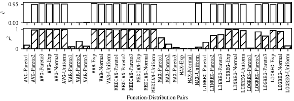
Figure 1: Applicability Evaluation for Function-Distribution Pairs. Cases where the bootstrap is theoretically inconsistent are underlined.

Figure 1 shows our results for all function-distribution pairs described above. The function-distribution pairs underlined are the cases where the bootstrap cannot estimate the approximation error correctly (i.e., Lemma 3 does not apply). The upper plot shows the simulated confidence for all cases, and the lower plot demonstrates the corresponding $r^{2}$ scores. Ideally, the simulated confidence should be close to $1-\delta=0.95$, and the $r^{2}$ score should be close to $1$ when the algorithm performs satisfactorily. Otherwise, the simulated confidence would be far away from $0.95$, which indicates that the algorithm produces sample size either too small to be accurate, or too large to be efficient, and the $r^{2}$ score would be far away from $1$.

As seen in the results, our $L^{2}$Miss algorithm demonstrates its board applicability on a range of data generating distributions and analytical functions. Specifically, the algorithm finds optimal sample size accurately for $25$ out of $36$ cases. When the bootstrap guarantee to be consistent, i.e., the $21$ cases that are not underlined, the simulated confidence of our algorithm is close to $0.95$ and the $r^{2}$ score is close to $1$, meaning that it finds the optimal sample sizes accurately for these cases. For the cases that the bootstrap is not consistent, no closed-form method can be applied, while our algorithm is still accurate for the $4$ out of $15$ cases, for example, AVG-Pareto2. This is because not only that the variance of the approximate analytical result is not infinity since the data size is finite, but also that our algorithm uses an iterative approach to minimized the impact of noise.

6.2.2 Multi-group Data

In the second part, we evaluate our algorithm on the data consisting of two independent groups generated by two distributions respectively. Each case is denoted by a distribution-distribution name pair. The distributions used here are the same as that described in the beginning of this section, i.e., Pareto1, Pareto2, Pareto3, Exp, Normal, and Uniform. We choose the analytical function to be AVG, which is the most commonly used one. The data size is set to be $100$ million tuples for each group. For the parameters of the $L^{2}$Miss algorithm, we choose the relative error bound $\epsilon^{*}=0.01$ and others remain the same as the previous experiment described in Section 6.2.1.

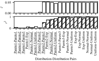
Figure 2: Applicability Evaluation for Averages of Distribution Pairs. Cases where the bootstrap is theoretically inconsistent are underlined.

Figure 2 shows the results of the experiment for all pairs of distributions. As described in Section 6.2.1, the underlined cases are the ones that bootstrap is not consistent theoretically. Since the two groups are generated independently, the bootstrap estimates the error consistently if and only if it is consistent for each group of the pair. Also, like in Figure 1, we plot the simulated confidence $\hat{c}$ and the $r^{2}$ score for all cases to figure out whether our algorithm produces the accurate sample sizes and whether our model depicts the relationship between the approximation error and the sample size effectively.

As shown in Figure 2, the $L^{2}$Miss algorithm demonstrates its capability to handle the $L^{2}$ norm error metric on various data. Specifically, among the $21$ total cases, the algorithm finds optimal sample sizes in $14$ cases. For the $10$ cases that the bootstrap is consistent, the algorithm returns accurate results, and the error model fits the error profile quite well. For other $11$ cases, such as Pareto2-Pareto3, even though the error estimation method is inconsistent, and the $r^{2}$ score is only around $0.5$, meaning that the model does not fit the profile perfectly, our algorithm also manage to find the optimal sample size accurately. This again shows the strong applicability of our algorithm in practice to almost all kinds of queries, even to those that is theoretically inapplicable.

In conclusion, the two applicability experiments above demonstrate that the $L^{2}$Miss algorithm can be applied to queries for which the error estimation method, i.e., the bootstrap, is theoretically consistent. For other queries that do not enjoy such a decent theoretical guarantee, few error estimation methods can be applied in theory, while our algorithm may still work well in practice. This gives users enough confidence to apply the algorithm to build an AQP system that is general enough to be applied to almost all kinds of analytical tasks, ranging from those as simple as finding averages to those as complicated as regression and classification.

6.3 Efficiency Evaluation

In this section, we study the efficiency of our algorithms. We compare the $L^{2}$Miss algorithm and its extensions against several state-of-the-art sampling-based AQP algorithms based on different error estimation methods. The AQP algorithms we evaluated include:

• The $L^{2}$Miss algorithm described in Algorithm 3 based on our MISS framework and uses the bootstrap for error estimation.

• The OrderMiss algorithm described in Section 5.3, which is also MISS-based and also employs the bootstrap to estimate errors.

• The Sample+Seek framework (SPS) proposed in [13], which uses Chernoff-type bounds for error estimation.

• Our implementation of the sample selection algorithm of BlinkDB [3] (BLK), which is based on the normality assumption to derive closed-form error estimation.

• The IFocus algorithm (IF) proposed in [23], which uses Hoeffding’s inequalities [19] for error estimation.

Among the five algorithms above, $L^{2}$Miss is compared with SPS and BLK since they all work with the $L^{2}$ norm error metric. OrderMiss is compared with IF, since both provide ordering guarantees. For $L^{2}$Miss and OrderMiss, since they require bootstrapping, we expect that their running time will be larger given that the total sample sizes are almost the same. SPS uses measure-biased sampling, which requires full scans on the data. Therefore, the running time will grow as the data size increases. BLK uses ad-hoc error estimation methods such that no estimation error exists. Therefore, BLK can be viewed as the best method as long as it can be applied.

The dataset is the TPC-H [1] and the factors evaluated include the relative error bound $\epsilon^{*}$, the error probability $\delta$, the number of groups of the data $m$, and the size of the dataset $N$. We define each query to have only one group-by attribute and one analytical attribute. In the queries, the relative error bound is varies from $0.01$ to $0.002$ and the error probability $\delta=0.1,0.05,0.01,0.005,0.001$ to evaluate their impact on performance. Moreover, tn order to evaluate the performance for multi-group queries, the group-by attributes used are LINESTATUS, RETURNFLAG, SHIPINSTRUCT, LINENUMBER, and TAX such that the numbers of groups of the data are $2$, $3$, $4$, $7$, and $9$ respectively. The analytical attribute is EXTENDEDPRICE. Each query involves only one group-by attribute and one analytical attribute. The data size is changed by modifying the scale factor of TPC-H. Specifically, $N$ is approximately the scale factor times $6\times 10^{6}$. The scale factors used include $1$, $10$, $30$, and $100$, which are officially designated by the TPC-H specification.

To measure efficiency, as mentioned at the beginning of this section, we measure both the running time and the total sample size $C\left(\boldsymbol{\mathbf{n}}\right)$ for each algorithm. As we always concern about accuracy, we also compute and plot the simulated confidence $\hat{c}$. To obtain more reliable results, when evaluating one factor, we control the others to keep as default. The default values are: $\epsilon^{*}=0.01$, $\delta=0.05$, $m=1$, $N=6\times 10^{6}$， i.e., the scale factor $=1$, and $f=\texttt{AVG}$, which is supported by all the five algorithms. For other parameters, $B=500$, $I_{n}=\left[1000,2000\right]$, and $l=5\left(m+1\right)$ where $m$ is the number of groups.

In the following experiments, all the algorithms are implemented by us in Python with multi-core support. The data and the index are loaded into the memory lazily (i.e., when they are accessed) for better performance. We use mmap(2) [22] to randomly access specific rows efficiently. All intermediate results are stored in memory to simplify our experiments.

6.3.1 $L^{2}$ Norm Error

First, we evaluate the performance of $L^{2}$Miss against SPS and BLK under the $L^{2}$ norm error metric. The results are shown in Figure 3. From the figure, we can learn that all algorithms achieve satisfactory accuracy in all test cases as the simulated confidence is around or above $1-\delta$.

Figure 3: Efficiency evaluation for algorithms that work under the $L^{2}$ norm error metric

Relative error bounds. Figure 3(a) shows the effect of varying relative error bound $\epsilon^{*}$. The running time and the total sample size of SPS is considerably larger than those of $L^{2}$Miss and BLK as expected. However, even though the total sample size of $L^{2}$Miss and BLK is quite similar, showing that $L^{2}$Miss is near-optimal in terms of total sample size. However, the running time of $L^{2}$Miss grows significantly faster than the others as the relative error bound decrease. This also coincides with our expectation since the bootstrap in $L^{2}$Miss is rather expensive. When the sampling rate is large, for example, at $~{}0.1$ when $\epsilon^{*}=0.002$, $L^{2}$Miss has no advantage over SPS.

Error probabilities. Figure 3(b) shows the performance with different error probabilities. This is similar to the case of varying $\epsilon^{*}$, i.e., $L^{2}$Miss is close to BLK, both in the running time and the total sample size, while they are both more than 3x faster than SPS. This shows that, when the sampling rate is small, for example, $\leq 0.01$, bootstrap-based methods can still be very efficient compared with those requiring full scans.

Number of groups. Figure 3(c) shows the performance on the data of different numbers of groups. As the number of group increases, both the running time and the total sample size of $L^{2}$Miss and BLK all increase while they remain the almost the same for SPS. This is because that $L^{2}$Miss and BLK consider groups separately, while SPS treats all the groups as a whole. Furthermore, the total sample size of BLK is considerably larger than that of $L^{2}$Miss. This is due to our naive implementation of BLK that we let the errors of all groups be the same, while we let $L^{2}$Miss determine the error distribution automatically to minimize the total sample size.

Data sizes. Figure 3(d) shows the effect on efficiency for different data sizes. As the data size grows, the running time and the total sample size increase rapidly for SPS, while for $L^{2}$Miss and BLK, they remain nearly unchanged. Note that when the data scale factor is $100$, the assumption that all intermediate results can be fit into memory fails to hold for SPS, resulting in a surge in the running time to around $3000$ seconds. (Note that at this point we only draw several samples to compute the simulated confidence for SPS since it is too time-consuming.) The reason is that SPS requires access all the data, while $L^{2}$Miss and BLK only need to access the sample data they draw. Therefore, when the sampling rate is small, $L^{2}$Miss and BLK are much more efficient than SPS.

In conclusion, our $L^{2}$Miss algorithm indeed finds optimal sample sizes compared with BLK and achieves satisfactory efficiency when the sampling rate is small, e.g., $\leq 0.01$, when the user would like to trade more accuracy for efficiency. On the other hand, SPS performs well when the sampling rate is large, e.g., $>0.1$, since it requires full scans. As for BLK, even though its performance seems perfect for all cases, it only supports simple aggregations such as AVG, COUNT, and VAR, while MISS supports almost all kinds of analytical functions.

6.3.2 Other Error Metrics

In this section, we focus on evaluating whether our extensions effectively supports other error metrics. Specifically, we focus on the performance of OrderMiss providing ordering guarantees compared with IF. To the best of our knowledge, IF is the only existing algorithm providing such guarantees.

Note that since different groups in the TPC-H dataset is rather identical in terms of their analytical results. Therefore, guaranteeing correct ordering properties would consume too much time and too large samples. Therefore, we add a bias to each group such that the analytical results of any two groups differ in a specific amount relative to the true analytical results, which are called the group bias. The group bias is set to $0.05$ by default, meaning that the difference of the analytical results in two adjacent groups in sorted order is about $0.05$ times their true results.

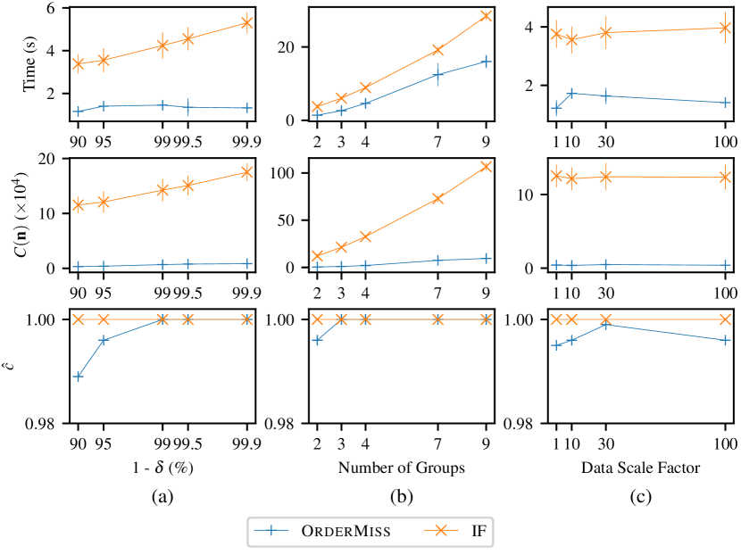
Figure 4: Efficiency evaluation for algorithms providing ordering guarantee

The results are presented in Figure 4. As observed from the third row of Figure 4, both OrderMiss and IF are able to produce accurate results, i.e., the correct ordering property holds with the given confidence. This indicates that our scheme, i.e., error bound conversion, successfully extends $L^{2}$Miss to support other error metrics.

In terms of efficiency, we can learn from Figure 4 that for different error probabilities, numbers of groups and data sizes, even though the two algorithms behave similarly in trend, our OrderMiss algorithm demonstrate its superiority against IF. Even though the bootstrap used by OrderMiss is costly, OrderMiss is still faster than IF since the total sample size of the former is several times smaller than the latter.

In summary, OrderMiss is much more efficient in providing ordering guarantees compared with IF, yet still ensuring accuracy. This is because MISS uses bootstrapping for error estimation, which is more accurate than concentration inequalities used by IF, resulting in great reduction in total sample size and the running time.

7 Related Work

In this section, we survey the algorithms related to AQP briefly.

Sample Selection for AQP. Since BlinkDB [3] was ever proposed, sampling-based AQP systems have been a hotspot in recent years in both industry and academia. Notable systems besides BlinkDB include iOLAP [38], Sample+Seek [13], and SnappyData [30]. However, only those who employ closed-form error estimation methods select suitable samples automatically, which is far from optimal or even inapplicable for many queries. Others, which use numerical error estimation methods, e.g., the bootstrap, do not equip with such mechanism, and users are required to create or select their desired samples manually. For example, SnappyData[30], which adopts the latter approach, requires users to create samples manually. It would select the largest one if more than one samples are available [21]. This approach limits its use to only experts. Our approach, on the contrary, determines the optimal sample size and draws the sample for each given query automatically, which makes it much easier to use.

AQP for complex queries. As noted in Section 2.1, we only consider simple analytical queries without selection and join in general in this paper. However, these two types of queries are essential to build a practical AQP system. Fortunately, our MISS framework is flexible enough to incorporate state-of-the-art techniques to gain such abilities. For joins, WanderJoin [26] is also a sampling-based technique that estimates the sampling probability for each tuples and relies on closed-form methods to estimate the approximation error for a analytical query. This method can be perfectly collaborated with our approach to produce overall approximate results directly to the end user. For selection, Sample+Seek [13] proposes an indexing scheme that accelerate selections in general using inverted indexing. This method is also compatible with our MISS framework and therefore can be directly incorporated into MISS to enable the MISS-based algorithms sample through an pre-built index.

AQP without sampling. Other AQP approaches without sampling include data cubes [17] and sketches[11] are also widely used. Nevertheless, these approaches are usually particularly designed for specific scenarios and have their own limitations. For example, data cubes are used when both the data and the query would not change much over time such that the pre-computed results are still valid. Sketches are for data streams and can only be applied to specific types of queries. On the contrary, our MISS framework and its derivative algorithms are designed to be suitable for as many types of queries as possible. By using online sampling and bootstrapping, our approach make almost no assumptions on the data and the query performed.

8 Conclusion and Future Work

In this paper, we propose the Model-based Iterative Sample Selection (MISS) frameworks and a family of algorithms based on the framework to find optimal sample sizes for various error metrics based on the error model that we build. Our approach not only supports $L^{2}$ norm error metric, but also provides other types of guarantees including bounded maximum error, bounded difference error and correct ordering under the MISS framework. With minor modifications, our algorithm can support various types of total sample size including uniformly or non-uniformly linear, polynomial and even exponential. We show theoretically and empirically that our algorithms can find near-optimal samples that satisfy user-defined error constraints for almost all kinds of data and user-defined analytical functions.

For future work, we see two directions that worth exploring. The first is to establish rigorous theories on what specific kinds of queries that our error model can be applied to, or even to find better error models. And the second is to build a practical and easy-to-use AQP system that incorporates our approaches and other techniques discussed in Section 7 to support arbitrary queries facing directly to end users.

References

- [1] Tpc-h benchmark. http://www.tpc.org/tpch/, 2017.
- [2] S. Agarwal, H. Milner, A. Kleiner, A. Talwalkar, M. I. Jordan, S. Madden, B. Mozafari, and I. Stoica. Knowing when you’re wrong: building fast and reliable approximate query processing systems. In International Conference on Management of Data, SIGMOD 2014, Snowbird, UT, USA, June 22-27, 2014, pages 481–492, 2014.
- [3] S. Agarwal, B. Mozafari, A. Panda, H. Milner, S. Madden, and I. Stoica. Blinkdb: queries with bounded errors and bounded response times on very large data. In Eighth Eurosys Conference 2013, EuroSys ’13, Prague, Czech Republic, April 14-17, 2013, pages 29–42, 2013.
- [4] D. Alabi and E. Wu. Pfunk-h: approximate query processing using perceptual models. In Proceedings of the Workshop on Human-In-the-Loop Data Analytics, HILDA@SIGMOD 2016, San Francisco, CA, USA, June 26 - July 01, 2016, page 10, 2016.
- [5] S. Amaran, N. V. Sahinidis, B. Sharda, and S. J. Bury. Simulation optimization: A review of algorithms and applications. CoRR, abs/1706.08591, 2017.
- [6] R. Bhatia and C. Davis. A better bound on the variance. The American Mathematical Monthly, 107(4):353–357, 2000.
- [7] G. E. P. Box and N. R. Draper. Empirical Model-building and Response Surface. John Wiley & Sons, Inc., New York, NY, USA, 1986.
- [8] G. Casella and R. L. Berger. Statistical Inference. Duxbury advanced series in statistics and decision sciences. Thomson Learning, 2002.
- [9] X. Chen. A New Generalization of Chebyshev Inequality for Random Vectors. ArXiv e-prints, July 2007.
- [10] F. Chung and L. Lu. Concentration inequalities and martingale inequalities: a survey. Internet Mathematics, 3(1):79–127, 2006.
- [11] G. Cormode. Data sketching. Commun. ACM, 60(9):48–55, 2017.
- [12] T. J. DiCiccio and B. Efron. Bootstrap confidence intervals. Statist. Sci., 11(3):189–228, 09 1996.
- [13] B. Ding, S. Huang, S. Chaudhuri, K. Chakrabarti, and C. Wang. Sample + seek: Approximating aggregates with distribution precision guarantee. In Proceedings of the 2016 International Conference on Management of Data, SIGMOD Conference 2016, San Francisco, CA, USA, June 26 - July 01, 2016, pages 679–694, 2016.
- [14] E. Erlandson. Faster random samples with gap sampling. http://erikerlandson.github.io/blog/2014/09/11/faster-random-samples-with-gap-sampling/, 2014.
- [15] J. Gryz, J. Guo, L. Liu, and C. Zuzarte. Query sampling in DB2 universal database. In Proceedings of the ACM SIGMOD International Conference on Management of Data, Paris, France, June 13-18, 2004, pages 839–843, 2004.
- [16] P. Hall. The Bootstrap and Edgeworth Expansion. Springer Series in Statistics. Springer New York, 1997.
- [17] J. M. Hellerstein, P. J. Haas, and H. J. Wang. Online aggregation. In SIGMOD 1997, Proceedings ACM SIGMOD International Conference on Management of Data, May 13-15, 1997, Tucson, Arizona, USA., pages 171–182, 1997.
- [18] W. Hoeffding. A class of statistics with asymptotically normal distribution. Ann. Math. Statist., 19(3):293–325, 09 1948.
- [19] W. Hoeffding. Probability inequalities for sums of bounded random variables. Journal of the American Statistical Association, 58(301):13–30, 1963.
- [20] P. J. Huber. Robust estimation of a location parameter. Ann. Math. Statist., 35(1):73–101, 03 1964.
- [21] S. Inc. Sample selection. https://snappydatainc.github.io/snappydata/sde/sample_selection/, 2017.
- [22] M. Kerrisk. The Linux Programming Interface. No Starch Press Series. No Starch Press, 2010.
- [23] A. Kim, E. Blais, A. G. Parameswaran, P. Indyk, S. Madden, and R. Rubinfeld. Rapid sampling for visualizations with ordering guarantees. PVLDB, 8(5):521–532, 2015.
- [24] E. Kreyszig. Introductory Functional Analysis with Applications. Wiley Classics Library. Wiley, 1989.
- [25] S. Krishnan, J. Wang, M. J. Franklin, K. Goldberg, and T. Kraska. Privateclean: Data cleaning and differential privacy. In Proceedings of the 2016 International Conference on Management of Data, SIGMOD Conference 2016, San Francisco, CA, USA, June 26 - July 01, 2016, pages 937–951, 2016.
- [26] F. Li, B. Wu, K. Yi, and Z. Zhao. Wander join: Online aggregation via random walks. In Proceedings of the 2016 International Conference on Management of Data, SIGMOD Conference 2016, San Francisco, CA, USA, June 26 - July 01, 2016, pages 615–629, 2016.
- [27] S. L. Lohr. Sampling: Design and Analysis. Advanced (Cengage Learning). Cengage Learning, 2009.
- [28] B. Mozafari. Approximate query engines: Commercial challenges and research opportunities. In Proceedings of the 2017 ACM International Conference on Management of Data, SIGMOD Conference 2017, Chicago, IL, USA, May 14-19, 2017, pages 521–524, 2017.
- [29] B. Mozafari and N. Niu. A handbook for building an approximate query engine. IEEE Data Eng. Bull., 38(3):3–29, 2015.
- [30] B. Mozafari, J. Ramnarayan, S. Menon, Y. Mahajan, S. Chakraborty, H. Bhanawat, and K. Bachhav. Snappydata: A unified cluster for streaming, transactions and interactice analytics. In CIDR 2017, 8th Biennial Conference on Innovative Data Systems Research, Chaminade, CA, USA, January 8-11, 2017, Online Proceedings, 2017.
- [31] J. Nocedal and S. Wright. Numerical Optimization. Springer Series in Operations Research and Financial Engineering. Springer New York, 2006.
- [32] A. W. van der Vaart. Asymptotic Statistics. Cambridge Series in Statistical and Probabilistic Mathematics. Cambridge University Press, 2000.
- [33] J. Wang, S. Krishnan, M. J. Franklin, K. Goldberg, T. Kraska, and T. Milo. A sample-and-clean framework for fast and accurate query processing on dirty data. In International Conference on Management of Data, SIGMOD 2014, Snowbird, UT, USA, June 22-27, 2014, pages 469–480, 2014.
- [34] J. Wang, C. Lin, R. He, M. Chae, Y. Papakonstantinou, and S. Swanson. MILC: inverted list compression in memory. PVLDB, 10(8):853–864, 2017.
- [35] L. Wasserman. All of Statistics: A Concise Course in Statistical Inference. Springer Texts in Statistics. Springer New York, 2004.
- [36] L. Wasserman. All of Nonparametric Statistics. Springer Texts in Statistics. Springer New York, 2006.
- [37] M. Zaharia, M. Chowdhury, T. Das, A. Dave, J. Ma, M. McCauly, M. J. Franklin, S. Shenker, and I. Stoica. Resilient distributed datasets: A fault-tolerant abstraction for in-memory cluster computing. In Proceedings of the 9th USENIX Symposium on Networked Systems Design and Implementation, NSDI 2012, San Jose, CA, USA, April 25-27, 2012, pages 15–28, 2012.
- [38] K. Zeng, S. Agarwal, and I. Stoica. iolap: Managing uncertainty for efficient incremental OLAP. In Proceedings of the 2016 International Conference on Management of Data, SIGMOD Conference 2016, San Francisco, CA, USA, June 26 - July 01, 2016, pages 1347–1361, 2016.
- [39] K. Zeng, S. Gao, B. Mozafari, and C. Zaniolo. The analytical bootstrap: a new method for fast error estimation in approximate query processing. In International Conference on Management of Data, SIGMOD 2014, Snowbird, UT, USA, June 22-27, 2014, pages 277–288, 2014.