Comment on scalar glueball mass

Abstract

We study the interaction of scalar glueball with quark-antiquark and four-quark spinless meson fields within the framework of a generalized linear sigma model in which the trace anomaly of QCD is exactly realized. To determine the pure scalar glueball mass ($m_{h}$), we consider the decoupling limit in which the scalar glueball decouples from the meson fields. We find the exact relationship $m_{h}=2\,h_{0}$ where $h_{0}$ is the vacuum expectation value of the scalar glueball field independent of the properties of the framework used.

The glueballs are the inherent byproducts of self-interacting gluons in QCD review . Since they can mix with meson fields of the same quantum numbers, determination of their properties becomes naturally challenging. The scalar glueballs are particularly difficult to study due to the fact that they have the quantum numbers of QCD vacuum and can induce spontaneous chiral symmetry breaking by developing vacuum expectation values. There have been an extensive investigation of glueballs from different approaches, including lattice QCD lattice , QCD sum-rules QCDSR ; Narrison and chiral models chiral .

We probe scalar glueballs within the framework of the generalized linear sigma model of glsm1 ; glsm2 in which the properties of scalar and pseudoscalar mesons below and above 1 GeV and their underlying quark-antiquark and four-quark mixings have been extensively studied. In this work we are specifically interested in properties of the lightest pure scalar glueball, hence, we consider a limit of the generalized linear sigma model in which the glueballs decouple from the quark-antiquark and four-quark states. The model is constructed in terms of 3$\times$3 matrix chiral nonet fields:

$$M=S+i\phi,\hskip 56.9055ptM^{\prime}=S^{\prime}+i\phi^{\prime},$$ (1)

where $M$ and $M^{\prime}$ transform in the same way under chiral SU(3) transformations

$$M \rightarrow U_{L}\,M\,U_{R}^{\dagger},$$

$$M^{\prime} \rightarrow U_{L}\,M^{\prime}\,U_{R}^{\dagger},$$ (2)

but transform differently under U(1)_A transformation properties

$$M \rightarrow e^{2i\nu}\,M,$$

$$M^{\prime} \rightarrow e^{-4i\nu}\,M^{\prime}.$$ (3)

$M$ contains the “bare” (unmixed) quark-antiquark scalar nonet $S$ and pseudoscalar nonet $\phi$, while $M^{\prime}$ contains “bare” two quarks and two antiquarks scalar nonet $S^{\prime}$ and pseudoscalar nonet $\phi^{\prime}$. The model distinguishes $M$ from $M^{\prime}$ through the U(1)_A transformation.

The Lagrangian density has the following general structure in terms of chiral nonets $M$ and $M^{\prime}$ as well as scalar glueball $h$ and pseudoscalar glueball $g$:

$${\cal L} = -\frac{1}{2}{\rm Tr}(\partial^{\mu}M\partial_{\mu}M^{\dagger})-\frac{1}{2}{\rm Tr}(\partial^{\mu}M^{\prime}\partial_{\mu}{M^{\prime}}^{\dagger})-V,$$

$$-V = f+f_{\rm A}+f_{\rm S}+f_{\rm SB}.$$ (4)

Here $f$ is a general function of fields $M$, $M^{\prime}$, $h$ and $g$ and is chiral, U(1)_A and scale invariant; $f_{\rm A}$ and $f_{\rm S}$ exactly mock up the axial and trace anomalies and $f_{\rm SB}$ introduces explicit breaking of the chiral symmetry due to quark masses. The leading choice of terms corresponds to eight or fewer underlying quark plus antiquark lines at each effective vertex glsm1 ; glsm2 and are as follows:

$$f(M,M^{\prime},g,h) = -\left(u_{1}h^{2}{\rm Tr}[MM^{\dagger}]+u_{2}{\rm Tr}[MM^{\dagger}MM^{\dagger}]\right.$$ (5)

$$\hskip 14.22636pt+u_{3}h^{2}{\rm Tr}[M^{\prime}M^{\prime\dagger}]$$

$$\hskip 14.22636pt+u_{4}h(\epsilon_{abc}\epsilon^{def}M^{a}_{d}M^{b}_{e}M^{\prime c}_{f}+h.c.)$$

$$\left.\hskip 14.22636pt+u_{5}h^{4}+u_{6}h^{2}g^{2}+\cdots\right),$$

$$f_{\rm A}=i{G\over 12}\left[\gamma_{1}\ln\left(\frac{\det M}{\det M^{\dagger}}\right)+\gamma_{2}\ln\left(\frac{{\rm Tr}(MM^{\prime\dagger})}{{\rm Tr}(M^{\prime}M^{\dagger})}\right)\right],$$ (6)

where $G=h^{3}g$ and $\gamma_{1}$ and $\gamma_{2}$ are arbitrary parameters that must satisfy the constraint $\gamma_{1}+\gamma_{2}=1$.

$$f_{\rm S}=-H \left\{\lambda_{1}\ln\left(\frac{H}{\Lambda^{4}}\right)\right.$$

$$+\lambda_{2}\left[\ln\left(\frac{\det M}{\Lambda^{3}}\right)+\ln\left(\frac{\det M^{\dagger}}{\Lambda^{3}}\right)\right]$$

$$\left.+\lambda_{3}\left[\ln\left(\frac{{\rm Tr}MM^{\prime\dagger}}{\Lambda^{2}}\right)+\ln\left(\frac{{\rm Tr}M^{\prime}M^{\dagger}}{\Lambda^{2}}\right)\right]\right\}.$$

where $\Lambda$ is the characteristic scale, $H=h^{4}$ and $\lambda_{1}$, $\lambda_{2}$ and $\lambda_{3}$ satisfying the constraint $4\lambda_{1}+6\lambda_{2}+4\lambda_{3}=1$. The two terms $f_{\rm A}$ and $f_{\rm S}$ ensure that the effective Lagrangian exactly satisfies the U(1)_A and the trace anomalies according to:

$$\partial^{\mu}J^{5}_{\mu}=\frac{g^{2}}{16\pi^{2}}N_{F}\tilde{F}F=G,$$

$$\theta^{\mu}_{\mu}=\partial^{\mu}D_{\mu}=-\frac{\beta(g^{2})}{2g}FF=H,$$ (8)

where $F$ is the SU(3)_C field tensor, $\tilde{F}$ is its dual, $N_{F}$ is the number of flavors, $\beta(g^{2})$ is the beta function for the coupling constant, $J^{5}_{\mu}$ is the axial current and $D_{\mu}$ is the dilatation current. The symmetry breaking term takes the simple form:

$$f_{\rm SB}=2{\rm Tr}[AS],$$ (9)

where $A={\rm diag}(A_{1},A_{2},A_{3})$ is a matrix proportional to the three light quark masses.

The isosinglet scalar states $f_{1}\cdots f_{5}$ are a linear combination of the following five components: two- and four-quark building blocks as well as a glueball component:

$$(i)\hskip 28.45274ptf_{a} = \frac{S^{1}_{1}+S^{2}_{2}}{\sqrt{2}}\hskip 19.91684pt\propto\hskip 14.22636ptn{\bar{n}},$$

$$(ii)\hskip 28.45274ptf_{b} = S^{3}_{3}\hskip 45.52458pt\propto\hskip 14.22636pts{\bar{s}},$$

$$(iii)\hskip 28.45274ptf_{c} = \frac{S^{\prime 1}_{1}+S^{\prime 2}_{2}}{\sqrt{2}}\hskip 14.22636pt\propto\hskip 14.22636ptns{\bar{n}}{\bar{s}},$$

$$(iv)\hskip 28.45274ptf_{d} = S^{\prime 3}_{3}\hskip 42.67912pt\propto\hskip 14.22636ptnn{\bar{n}}{\bar{n}},$$

$$(v)\hskip 28.45274pth,$$ (10)

where the non-strange ($n$) and strange ($s$) quark content for each basis state has been listed at the end of each line above. The VEV of the scalar fields

$$\alpha_{a} = \langle S_{a}^{a}\rangle,$$

$$\beta_{a} = \langle{S^{\prime}}_{a}^{a}\rangle,$$

$$h_{0} = \langle h\rangle,$$ (11)

with $a=1\cdots 3$ spontaneously break chiral symmetry.

The minimum equations that determine the vacuum of the model are obtained from equations:

$$\left\langle{{\partial V}\over{\partial S_{1}^{1}}}\right\rangle_{0} = 0,$$

$$\left\langle{{\partial V}\over{\partial S_{3}^{3}}}\right\rangle_{0} = 0,$$

$$\left\langle{{\partial V}\over{\partial{S^{\prime}}_{1}^{1}}}\right\rangle_{0} = 0,$$

$$\left\langle{{\partial V}\over{\partial{S^{\prime}}_{3}^{3}}}\right\rangle_{0} = 0,$$

$$\left\langle{{\partial V}\over{\partial h}}\right\rangle_{0} = 0,$$ (12)

where brackets with subscript zero represent evaluation of each derivative at VEV values of (11).

In order to extract the properties of the scalar glueball, we consider the decoupling limit in which the scalar glueball decouples from quark mesons:

$$\left\langle{{\partial^{2}V}\over{\partial S_{1}^{1}\,\partial h}}\right\rangle_{0} = 4\sqrt{2}u_{4}[\beta_{1}\alpha_{3}+\alpha_{1}\beta_{3}]+4\sqrt{2}u_{1}h_{0}\alpha_{1}$$

$$+\frac{8\sqrt{2}h_{0}^{3}\lambda_{2}}{\alpha_{1}}+\frac{8\sqrt{2}h_{0}^{3}\lambda_{3}\beta_{1}}{2\alpha_{1}\beta_{1}+\alpha_{3}\beta_{3}}=0,$$

$$\left\langle{{\partial^{2}V}\over{\partial S_{3}^{3}\,\partial h}}\right\rangle_{0} = 8u_{4}\alpha_{1}\beta_{1}+4u_{1}h_{0}\alpha_{3}+\frac{8h_{0}^{3}\lambda_{2}}{\alpha_{3}}$$

$$+\frac{8h_{0}^{3}\lambda_{3}\beta_{3}}{2\alpha_{1}\beta_{1}+\alpha_{3}\beta_{3}}=0,$$

$$\left\langle{{\partial^{2}V}\over{\partial{S^{\prime}}_{1}^{1}\,\partial h}}\right\rangle_{0} = 4\sqrt{2}\alpha_{1}\alpha_{3}u_{4}+4\sqrt{2}u_{3}h_{0}\beta_{1}$$

$$+\frac{8\sqrt{2}h_{0}^{3}\lambda_{3}\alpha_{1}}{2\alpha_{1}\beta_{1}+\alpha_{3}\beta_{3}}=0,$$

$$\left\langle{{\partial^{2}V}\over{\partial{S^{\prime}}_{3}^{3}\,\partial h}}\right\rangle_{0} = 4\alpha_{1}^{2}u_{4}+4u_{3}h_{0}\beta_{3}$$ (13)

$$+\frac{8h_{0}^{3}\lambda_{3}\alpha_{3}}{2\alpha_{1}\beta_{1}+\alpha_{3}\beta_{3}}=0.$$

The first two minimum equations in (12) can be used to solve for $A_{1}$ and $A_{3}$ in terms of other parameters. The third and fourth equations in (12) give:

$$4\alpha_{1}^{2}\alpha_{3}\beta_{1}u_{4}+2\alpha_{3}^{2}\beta_{3}\alpha_{1}u_{4}+2\beta_{1}^{2}\alpha_{1}h_{0}u_{3}$$

$$+h_{0}^{3}\lambda_{3}\alpha_{1}+\alpha_{3}\beta_{1}\beta_{3}h_{0}u_{3}=0,$$

$$4\alpha_{1}^{3}\beta_{1}u_{4}+2\alpha_{1}^{2}\alpha_{3}\beta_{3}u_{4}+2\alpha_{1}\beta_{1}\beta_{3}h_{0}u_{3}$$

$$+\alpha_{3}\beta_{3}^{2}h_{0}u_{3}+\alpha_{3}h_{0}^{3}\lambda_{3}=0.$$ (14)

Solving this system results in relationships:

$$\alpha_{3}=\alpha_{1}=\alpha,$$

$$\beta_{3}=\beta_{1}=\beta,$$ (15)

and consequently $A_{1}=A_{3}=A$, and shows that in the decoupling limit the chiral symmetry breaks into its SU(3)_V subgroup. Furthermore, taking the decoupling equations (13) into account, we find additional relationships between the model parameters:

$$u_{3} = -\frac{3\alpha^{2}u_{4}}{\beta h_{0}},$$

$$\lambda_{2} = -\frac{\alpha^{2}(h_{0}u_{1}+4\beta u_{4})}{2h_{0}^{3}},$$

$$\lambda_{3} = \frac{3\alpha^{2}\beta u_{4}}{h_{0}^{3}}.$$ (16)

The scalar glueball mass is determined from

$$m_{h}^{2}=\left\langle{{\partial^{2}V}\over{\partial^{2}h}}\right\rangle_{0},$$ (17)

where, in the decoupling limit, becomes

$$m_{h}^{2} = 6\,u_{1}\,\alpha^{2}+6\,u_{3}\,\beta^{2}+12\,u_{5}\,h_{0}^{2}+28\,{{\it h_{0}}}^{2}\lambda_{1}$$ (18)

$$+12\,h_{0}^{2}\left[\lambda_{1}\,\ln\left({\frac{h_{0}^{4}}{\Lambda^{4}}}\right)+2\,\lambda_{2}\,\ln\left({\frac{\alpha^{3}}{{\Lambda}^{3}}}\right)\right.$$

$$\left.+2\,\lambda 3\,\ln\left({\frac{3\,\alpha\,\beta}{{\Lambda}^{2}}}\right)\right].$$

The fifth equation in (12) can be used to solve for $u_{5}$ in terms of other parameters, which upon substituting this solution back into (18), the glueball mass squared simplifies to:

$$m_{h}^{2} = {1\over h_{0}}\left(-36\,{\alpha}^{2}\beta\,u_{4}-12\,u_{3}\,h_{0}\,\beta^{2}-12\,u_{1}\,h_{0}\,\alpha^{2}\right.$$ (19)

$$\left.+16\,h_{0}^{3}\lambda_{1}\right).$$

The first two terms cancel out exactly using the first relation in (16). Using the other two relations in (16), simplifies the third and the fourth terms in (19):

$$m_{h}^{2} = -12\,u_{1}\,\alpha^{2}+16\,h_{0}^{2}\lambda_{1}$$ (20)

$$= -12\alpha^{2}\left({{-2h_{0}^{2}\,\lambda_{2}}\over{\alpha^{2}}}-{{4\beta\,u_{4}}\over{h_{0}}}\right)+16\,h_{0}^{2}\lambda_{1}$$

$$= 24h_{0}^{2}\lambda_{2}+48{{\beta\alpha^{2}u_{4}}\over h_{0}}+16\,h_{0}^{2}\,\lambda_{1}$$

$$= 4h_{0}^{2}\left(4\lambda_{1}+6\lambda_{2}+4\lambda_{3}\right).$$

The parenthesis is equal to 1 [see (LABEL:scale_anm)] leading to a simple relationship for the pure glueball mass.

$$m_{h}=2h_{0}.$$ (21)

Note that this result which was derived for a specific potential is model independent. This can be shown by directly examining the trace anomaly for a generic potential $V$ which contains the fields $M$, $M^{\prime}$, $h$ and $g$. Requiring that the scale transformation of $V$ exactly gives the second equation of (8), yields

$$\left[M_{ij}\frac{\partial V}{\partial M_{ij}}+M_{ij}^{\prime}\frac{\partial V}{\partial M^{\prime}_{ij}}+h.c.\right]+\frac{\partial V}{\partial h}h+\frac{\partial V}{\partial g}g-4V=h^{4}.$$

(22)

Differentiating with respect to the field $h$ and taking the vacuum expectation values results in

$$\left[\left\langle M_{ij}\right\rangle_{0}\left\langle\frac{\partial^{2}V}{\partial M_{ij}\partial h}\right\rangle_{0}+\left\langle M_{ij}^{\prime}\right\rangle_{0}\left\langle\frac{\partial^{2}V}{\partial M^{\prime}_{ij}\partial h}\right\rangle_{0}+h.c.\right]$$

$$+\left\langle\frac{\partial^{2}V}{\partial h^{2}}\right\rangle_{0}h_{0}+\left\langle\frac{\partial V}{\partial h}\right\rangle_{0}+\left\langle\frac{\partial^{2}V}{\partial g\partial h}\right\rangle_{0}\left\langle g\right\rangle_{0}-\left\langle 4\frac{\partial V}{\partial h}\right\rangle_{0}$$

$$=4h_{0}^{3}.$$ (23)

In the decoupling limit of (16), the square bracket vanishes. The first term after the square bracket is the scalar glueball mass squared times $h_{0}$, terms including $\left\langle\partial V/\partial h\right\rangle_{0}$ vanish because of minimum condition [the last Eq. in (12)] and $\left\langle g\right\rangle_{0}$ vanishes because of parity, resulting in the same conclusion as in (21).

Although relationship (21) can be derived model independently, computation of $h_{0}$ requires specific modeling of the potential. In first approximation,

$$h_{0}^{4}\approx h_{x}^{4}=\langle h^{4}\rangle=\langle H\rangle=\left\langle-\frac{\beta(g)}{2g}G^{2}\right\rangle=\frac{9}{8\pi}\left\langle\alpha_{s}G^{2}\right\rangle,$$

(24)

where the gluon condensate can be imported from QCD sum-rules or lattice QCD. However, the relationship between $h_{0}$ and $h_{x}$ should be established more carefully. The partition function for our model reads:

$$Z=\int dhdgdMdM^{\prime}\exp[i\int d^{4}x{\cal L}(h,g,M,M^{\prime})].$$ (25)

Making a change of variables from $h$ and $g$ to $H=h^{4}$ and $G=h^{3}g$, with the Jacobian of the transformation

$$J(x-y)=\det\left[H(x)^{-3/2}\delta(x-y)\right],$$ (26)

the minimum equation for $H$ then becomes:

$$\frac{\partial iS}{\partial H(z)}-{3\over 2}\frac{1}{H(z)}\delta(0)=0.$$ (27)

Here $S$ is the action and the second term comes from the differentiation of the determinant in Eq. (26). Eq. (27) can be rewritten as:

$$\int d^{4}y\frac{\partial iS}{\partial h(y)}\frac{\partial h(y)}{\partial H(z)}-{3\over 2}\frac{1}{H(z)}\delta(0)=0,$$ (28)

which becomes:

$$-i\frac{\partial V(z)}{\partial h(z)}\frac{1}{4H(z)^{3/4}}-{3\over 2}\frac{1}{H(z)}\delta(0)=0.$$ (29)

Note that this time the derivative is not taken in the functional sense. The $\delta$ function in Eq. (29) needs regularization. Since we are interested in a small range of values around the vacuum condensate we can write:

$$\delta(0) = \lim_{x\rightarrow y}\delta(x-y)$$

$$= \int\frac{d^{4}k}{(2\pi)^{4}}\exp\left(\frac{\partial^{2}}{m_{c}^{4}}\right)\exp[-ik(x-y)]=i\frac{m_{c}^{4}}{16\pi^{2}},$$

where the integral is computed in the Euclidean space and $m_{c}$ is an appropriate cut-off scale for a linear sigma model with three flavors. Then the vacuum equation (29) becomes:

$$\frac{\partial V}{\partial h}\Bigg{|}_{h=h_{x}}\frac{1}{4h_{x}^{3}}+\frac{6}{64\pi^{2}}\frac{m_{c}^{4}}{h_{x}^{4}}=0.$$ (31)

We multiply the above equation by $4$ and subtract form it the vacuum equation for $h_{0}$ divided by $h_{0}^{3}$ to get:

$$K(h_{0})=\frac{\partial V}{\partial h}\Bigg{|}_{h=h_{x}}\frac{1}{h_{x}^{3}}+\frac{6}{16\pi^{2}}\frac{m_{c}^{4}}{h_{x}^{4}}-\frac{\partial V}{\partial h}\Bigg{|}_{h=h_{0}}\frac{1}{h_{0}^{3}}=0.$$

In the decoupling limit that we considered here, this equation can be rewritten in terms of the model parameters

$$K(h_{0}) = 4\lambda_{1}\ln\left(\frac{h_{x}^{4}}{h_{0}^{4}}\right)+(6\alpha^{2}u_{1}+6\beta^{2}u_{3})\left(\frac{1}{h_{x}^{2}}-\frac{1}{h_{0}^{2}}\right)$$ (33)

$$+12u_{4}\alpha^{2}\beta\left(\frac{1}{h_{x}^{3}}-\frac{1}{h_{0}^{3}}\right)+\frac{6}{16\pi^{2}}\frac{m_{c}^{4}}{h_{x}^{4}}=0.$$

In this equation, $h_{x}$ is an input, computed from Eq. (24) with the value of the gluon condensate taken from QCD sum-rules or lattice QCD. (There is a large discrepancy between the values of gluon condensate given by lattice QCD and QCD sum-rules.) The cut off $m_{c}$ is adjusted such that $K=0$ occurs at a stable point (the local minimum of $K$ at which there is no sensitivity to determination of $h_{0}$). For example, from QCD sum-rule analysis of Narrison :

$$\langle\alpha_{s}G^{2}\rangle=(0.070\pm 0.013)\,\,{\rm GeV}^{4},$$ (34)

which gives $h_{x}^{\rm min}=0.057$ GeV and $h_{x}^{\rm max}=0.083$ GeV, function $K$ vanishes at a local minimum if $m_{c}$ = 1.04 GeV and 1.14 GeV, respectively, as shown in Fig. 1. At these local minima $h_{0}$ is 0.887 GeV and 0.974 GeV, respectively. These values of $h_{0}$, when entered into Eq. (21), result in a pure scalar glueball mass of 1.77 GeV and 1.95 GeV, overlapping with some of the estimates in the literature lattice ; chiral .

In summary, this work presented a model independent relationship between the mass and the condensate of a pure scalar glueball. This relationship can be of a key importance in low-energy QCD analyses by bridging frameworks involving quarks and gluons to hadronic models of low-energy QCD.

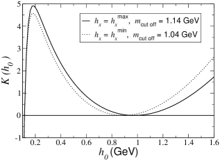
Figure 1: Function $K(h_{0})$ [Eq. (33)] versus $h_{0}$ with the two values of $h_{x}$, its minimum (dotted line) and its maximum (solid line) extracted from QCD sum-rule analysis of Narrison . For each case, the cut off values are adjusted such that $K=0$ occurs at its minimum which is insensitive to extraction of $h_{0}$. At the two minima, the values of $h_{0}$ are 0.887 and 0.974 GeV corresponding to the minimum and maximum values of $h_{x}$, respectively.

References

• (1) C. Patrignani et al. (Particle Data Group), Chin. Phys. C, 40, 100001 (2016); E. Klempt and A. Zaitsev, Phys. Rept. 454, 1 (2007).
• (2) C.J. Morningstar and M.J. Peardon, Phys. Rev. D 60, 034509 (1999); W.J. Lee and D. Weingarten, Phys. Rev. D 61, 014015 (2000); G. S Bali et al., Phys. Lett. B 309, 379 (1993); C. McNeile et al. [UKQCD Collaboration], Phys. Rev. D 63, 114503 (2001); L.C. Gui et al. [CLQCD Collaboration], Phys. Rev. Lett.  110, no. 2, 021601 (2013).
• (3) M.A. Shifman, A.I. Vainshtein and V.I. Zakharov, Nucl. Phys. B 147, 385, 448 (1979); S. Narison and G. Veneziano, Int. J. Mod. Phys. A 4, 2751 (1981); S. Narison, Z. Phys. C 26, 209 (1984).
• (4) S. Narison, Phys. Lett. B 706, 412-422 (2012).
• (5) M. Albaladejo and J.A. Oller, Phys. Rev. Lett.  101, 252002 (2008); F. Giacosa, T. Gutsche, V.E. Lyubovitskij and A. Faessler, Phys. Rev. D 72, 094006 (2005); M. Chanowitz, Phys. Rev. Lett.  95, 172001 (2005); A.H. Fariborz, Int. J. Mod. Phys. A 19, 2095 (2004); A.H. Fariborz, Phys. Rev. D 74, 054030 (2006); C. Amsler and F.E. Close, Phys. Rev. D 53, 295 (1996).
• (6) A.H. Fariborz, R. Jora and J. Schechter, Phys. Rev. D 72, 034001 (2005); Phys. Rev. D 76, 014011 (2007); Phys. Rev. D 76, 114001 (2007); Phys. Rev. D 77, 034006 (2008); Phys. Rev. D 79, 074014 (2009).
• (7) A.H. Fariborz and R. Jora, Phys. Rev. D 96, 096021 (2017); Phys. Rev. D 95, 116003 (2017); Phys. Rev. D 95, 114001 (2017).