Optimal Hölder-Zygmund exponent of semi-regular refinable functions

Abstract

The regularity of refinable functions has been investigated deeply in the past 25 years using Fourier analysis, wavelet analysis, restricted and joint spectral radii techniques. However the shift-invariance of the underlying regular setting is crucial for these approaches. We propose an efficient method based on wavelet tight frame decomposition techniques for estimating Hölder-Zygmund regularity of univariate semi-regular refinable functions generated, e.g., by subdivision schemes defined on semi-regular meshes $\displaystyle\mathbf{t}\;=\;-h_{\ell}\mathbb{N}\cup\{0\}\cup h_{r}\mathbb{N}$, $\displaystyle h_{\ell},h_{r}\in(0,\infty)$. To ensure the optimality of this method, we provide a new characterization of Hölder-Zygmund spaces based on suitable irregular wavelet tight frames. Furthermore, we present proper tools for computing the corresponding frame coefficients in the semi-regular setting. We also propose a new numerical approach for estimating the optimal Hölder-Zygmund exponent of refinable functions which is more efficient than the linear regression method. We illustrate our results with several examples of known and new semi-regular subdivision schemes with a potential use in blending curve design.

Classification (MSCS): 42C40, 42C15, 65D17

1 Introduction and notation

This paper presents a fast and efficient method for computing the optimal (critical) Hölder-Zygmund regularity of a certain class of non-shift-invariant univariate refinable functions, the so-called semi-regular refinable functions generated e.g. by binary subdivision [12, 29] defined on the meshes

$${\mathbf{t}}\;=\;-h_{\ell}\mathbb{N}\cup\{0\}\cup h_{r}\mathbb{N},\quad h_{\ell},h_{r}\in(0,\infty).$$ (1)

It is well known that a family $\displaystyle\{\phi_{k}\,:\,k\in\mathbb{Z}\}$ of refinable functions $\displaystyle\phi_{k}\in L_{2}(\mathbb{R})$ assembled in a bi-infinite column vector $\displaystyle\Phi=[\phi_{k}\,:\,k\in\mathbb{Z}]$ satisfies the refinement equation

$$\Phi=\mathbf{P}\,\Phi(2\cdot)$$ (2)

with a real-valued bi-infinite matrix $\displaystyle\mathbf{P}$. In the semi-regular case, finitely many (corresponding to a certain neighborhood of the origin) of the elements in $\displaystyle\Phi$ can not be expressed as integer shifts of any other function in $\displaystyle\Phi$ and (2) reduces to finitely many different scalar-valued refinement equations. The assumption (1) on the mesh becomes vital only in Section 4.

Our method relies on a new characterization of Hölder-Zygmund spaces. It generalizes successful wavelet frame methods [5, 7, 6, 11, 17, 23, 25, 26] from the regular to the semi-regular and even to the irregular setting and is the first step towards a better understanding of regularity at extraordinary vertices [24, 30] in the bivariate case. In comparison to the method in [12], our approach yields numerical estimates for the optimal Hölder-Zygmund regularity of a refinable function without requiring any ad hoc regularity estimates for the corresponding subdivision scheme. Our numerical estimates turn out to be optimal in all considered cases and require fewer computational steps than the standard linear regression method.

In the regular case, the wavelet frame methods rely on the characterization of Besov spaces $\displaystyle B^{r}_{p,q}(\mathbb{R})$ provided by Lemarié and Meyer [21] in their follow-up on the results by Frazier and Jawerth [15].

Theorem 1.1 ([23], Section 6.10).

Let $\displaystyle s>0$ and $\displaystyle 1\leq p,q\leq\infty$. Assume

$$\big{\{}\phi_{k}=\phi_{0}(\cdot-k)\ :\ k\in\mathbb{Z}\big{\}}\cup\big{\{}\psi_{j,k}=2^{(j-1)/2}\psi_{1,0}(2^{j-1}\cdot-k)\ :\ k\in\mathbb{Z},j\in\mathbb{N}\big{\}}\subset\mathcal{C}^{s}(\mathbb{R})$$

is a compactly supported orthogonal wavelet system with $\displaystyle v$ vanishing moments. Then, for $\displaystyle r\in(0,\min(s,v))$,

$$B^{r}_{p,q}(\mathbb{R})\;=\;\left\{\;\sum_{k\in\mathbb{Z}}a_{k}\phi_{k}+\sum_{j\in\mathbb{N}}\sum_{k\in\mathbb{Z}}b_{j,k}\psi_{j,k}\;:\;\{a_{k}\}_{k\in\mathbb{Z}}\in\ell_{p}(\mathbb{Z}),\ \left\{2^{j\left(r+\frac{1}{2}-\frac{1}{p}\right)}\left\|\{b_{j,k}\}_{k\in\mathbb{Z}}\right\|_{\ell_{p}}\;\right\}_{j\in\mathbb{N}}\in\ell_{q}(\mathbb{Z})\right\}.$$

To be able to apply Theorem 1.1, i.e. to extract the regularity of a given function $\displaystyle f$ from the decay of its coefficients $\displaystyle\{a_{k}=\langle f,\phi_{k}\rangle\ \,:\,k\in\mathbb{Z}\}$ and $\displaystyle\{b_{j,k}=\langle f,\psi_{j,k}\rangle\,:\,j\in\mathbb{N},\ k\in\mathbb{Z}\}$, one must first compute these inner products. In the context of subdivision, the analytic expressions neither of the analyzed function $\displaystyle f$ nor of the refinable functions $\displaystyle\phi_{k}$ are usually known. However, in the regular (shift-invariant) setting, the desired inner products can be computed explicitly (or numerically) using results of [18]. In the general non-shift-invariant case, the task becomes overwhelming and is far from being understood. In the semi-regular case, however, both the suitable wavelet tight frames exist, e.g. the ones generated by B-splines [8, 9] or by Dubuc-Deslauriers refinable functions [28], and, similarly to [22, 28], the corresponding frame coefficients can be computed.

However, Theorem 1.1 does not cover the case of semi-regular wavelet tight frames, since we lose the orthogonality and, most importantly, the shift-invariance. This paper provides a generalization of Theorem 1.1 for function systems

$$\mathcal{F}=\big{\{}\phi_{k}\,:\,k\in\mathbb{Z}\big{\}}\cup\big{\{}\psi_{j,k}\,:\,j\in\mathbb{N},\ k\in\mathbb{Z}\big{\}}$$ (3)

with the following properties

• $\displaystyle\mathcal{F}$ forms a (Parseval/normalized) tight frame for $\displaystyle L^{2}(\mathbb{R})$, i.e.

  $$f\;=\;\sum\limits_{k\in\mathbb{Z}}\;\langle f,\phi_{k}\rangle\phi_{k}\;+\;\sum\limits_{j\in\mathbb{N}}\;\sum\limits_{k\in\mathbb{Z}}\;\langle f,\psi_{j,k}\rangle\;\psi_{j,k},\quad f\in L^{2}(\mathbb{R});$$ (4)

• there exists a constant $\displaystyle C_{supp}>0$ such that

  $$\sup_{k\in\mathbb{Z}}\{|\mathop{\mathrm{supp}}(\phi_{k})|\}\;\leq\;C_{supp}\quad\textrm{and}\quad\sup_{k\in\mathbb{Z}}\{|\mathop{\mathrm{supp}}(\psi_{j,k})|\}\;\leq\;C_{supp}\;2^{-j},\quad j\in\mathbb{N};$$ (5)

• there exists a constant $\displaystyle C_{\Gamma}>0$ such that for every bounded interval $\displaystyle K\subset\mathbb{R}$ the sets

  $$\displaystyle\Gamma_{0}(K)\;=\;\{\;k\in\mathbb{Z}\;:\;\mathop{\mathrm{supp}}(\phi_{k})\cap K\;\not=\;\emptyset\;\}\quad\hbox{and}\quad\Gamma_{j}(K)\;=\;\{\;k\in\mathbb{Z}\;:\;\mathop{\mathrm{supp}}(\psi_{j,k})\cap K\;\not=\;\emptyset\;\},\quad j\in\mathbb{N},$$

  satisfy

  $$|\Gamma_{j}(K)|\;\leq\;C_{\Gamma}(2^{j}|K|+1),\quad j\geq 0;$$ (6)

• $\displaystyle\mathcal{F}$ has $\displaystyle v\in\mathbb{N}$ vanishing moments, i.e.

  $$\int_{\mathbb{R}}\;x^{n}\;\psi_{j,k}(x)\;dx\;=\;0,\quad n\in\{0,\dots,v-1\},\quad j\in\mathbb{N},\quad k\in\mathbb{Z},$$ (7)

  and there exists a sequence of points $\displaystyle\{x_{j,k}\,:\,j\in\mathbb{N},\ k\in\mathbb{Z}\}$ such that, for every $\displaystyle 0\leq r\leq v$, there exists a constant $\displaystyle C_{vm,r}>0$ such that

  $$\sup_{k\in\mathbb{Z}}\;\int_{\mathbb{R}}|x|^{r}|\psi_{j,k}(x+x_{j,k})|dx\;\leq\;C_{vm,r}\;2^{-j\left(r+\frac{1}{2}\right)};$$ (8)

• $\displaystyle\mathcal{F}\subset\mathcal{C}^{s}(\mathbb{R})$, $\displaystyle s>0$, and for every $\displaystyle 0\leq r\leq s$ there exists a constant $\displaystyle C_{sm,r}>0$ such that

  $$\sup_{k\in\mathbb{Z}}\{\|\phi_{k}\|_{\mathcal{C}^{r}}\}\;\leq\;C_{sm,r}\quad\textrm{and}\quad\sup_{k\in\mathbb{Z}}\{\|\psi_{j,k}\|_{\mathcal{C}^{r}}\}\;\leq\;C_{sm,r}\;2^{j\left(r+\frac{1}{2}\right)},\quad j\in\mathbb{N}.$$ (9)

Estimate (8) expresses localization condition for the framelets $\displaystyle\psi_{j,k}$. Note that (8) is implied by conditions (II) and (V) for $\displaystyle 0\leq r\leq s$. Indeed, choosing $\displaystyle x_{j,k}$ to be the midpoint of $\displaystyle\mathop{\mathrm{supp}}(\psi_{j,k})$, $\displaystyle j\in\mathbb{N}$, $\displaystyle k\in\mathbb{Z}$, we get

$$\int_{\mathbb{R}}\;|x|^{r}\;|\psi_{j,k}(x+x_{j,k})|dx\;\leq\;C_{sm,0}\;\left(\frac{|\mathop{\mathrm{supp}}(\psi_{j,k})|}{2}\right)^{r}\;2^{j/2}\;|\mathop{\mathrm{supp}}(\psi_{j,k})|\;\leq\;\frac{C_{supp}^{r+1}\;C_{sm,0}}{2^{r}}\;2^{-j\left(r+\frac{1}{2}\right)}.$$

We state the assumptions (II) and (V) separately to emphasize their duality, which becomes even more evident in the statements of Propositions 2.4 and 2.5 in Section 2. Indeed, Theorems 1.1 and 1.2 require $\displaystyle 0<r<\min(s,v)$, where the value of $\displaystyle s$ or $\displaystyle v$ affects only one of the inclusions in either Proposition 2.4 or in Proposition 2.5. Moreover, stating (IV) and (V) separately, we can easily generalize our results to the case of dual frames with the analysis frame satisfying (II) and (IV) and the synthesis frame satisfying (III) and (V). In the regular case, a natural choice in (8) is $\displaystyle x_{j,k}=2^{-j}k$. In general, even if the system $\displaystyle\mathcal{F}$ is non-shift-invariant, the points $\displaystyle x_{j,k}$ ensure the quasi-uniform (standard concept in the context of spline and finite element methods) behavior of the framelets over $\displaystyle\mathbb{R}$ and act as the center for every element $\displaystyle\psi_{j,k}$. The other assumptions also manifest the quasi-uniform behavior of the framelets over $\displaystyle\mathbb{R}$.

The setting described by assumptions (I)-(V) includes some cases not addressed in the results of Frazier and Jawerth [15] or of Cordero and Gröchenig in [10]. The results of [15] require that the elements of $\displaystyle\mathcal{F}$ in the decomposition of $\displaystyle B^{r}_{p,q}(\mathbb{R})$ are linked to dyadic intervals. The results in [10] impose the so-called localization property which implies that the system $\displaystyle\mathcal{F}$ is semi-orthogonal (in particular, non-redundant).

On the other hand, one could view the quite natural and application oriented assumptions (I)-(V) to be somewhat restrictive, since these assumptions were designed to fit wavelet tight frames $\displaystyle\mathcal{F}$ constructed using results of [9]. For such function families $\displaystyle\mathcal{F}$, there exists a sequence of bi-infinite matrices $\displaystyle\{\mathbf{Q}_{j}\,:\,j\in\mathbb{N}\}$ such that the column vectors

$$\Psi_{j}=[\psi_{j,k}\,:\,k\in\mathbb{Z}],\quad j\in\mathbb{N},\quad\hbox{and}\quad\Phi=[\phi_{k}\,:\,k\in\mathbb{Z}]$$

satisfy

$$\Psi_{j}\;=\;2^{j/2}\;\mathbf{Q}_{j}^{T}\;\Phi(2^{j}\cdot),\quad j\in\mathbb{N}.$$ (10)

Such bi-infinite matrices $\displaystyle\{\mathbf{Q}_{j}\,:\,j\in\mathbb{N}\}$ are e.g the ones constructed in [28] for the family of Dubuc-Deslauriers subdivision schemes [1, 2, 13]. For function families $\displaystyle\mathcal{F}$ satisfying (3), assumptions (II)-(V) reflect the properties of the matrices $\displaystyle\{\mathbf{Q}_{j}\,:\,j\in\mathbb{N}\}$: (II) controls the support of the columns of the $\displaystyle\mathbf{Q}_{j}$s, (III) controls the slantedness of the $\displaystyle\mathbf{Q}_{j}$s and (IV) and (V) are linked to eigenproperties of the $\displaystyle\mathbf{Q}_{j}$s.

Nevertheless, the spirit of assumptions (I)-(V) merges with the spirit of atoms and molecules in [15] and compactly supported orthogonal wavelet systems, for which (I)-(V) are also satisfied. These similarities are also visible in the structure of the proofs of Propositions 2.4 and 2.5.

For the sake of completeness, we point out that our setting includes some of the wavelet frames considered in [16] for which a characterization of the spaces $\displaystyle B^{r}_{2,2}(\mathbf{R})$, $\displaystyle r\in\mathbb{R}$, is given. However, those frames are shift-invariant, i.e (3) holds with block $\displaystyle 2$-slanted $\displaystyle\{\mathbf{Q}_{j}\,:\,j\in\mathbb{N}\}$. The approach in [16] applies Fourier techniques that are not feasible in our case, due to the lack of shift-invariance. The lack of shift-invariance makes also the techniques in [3] inapplicable in our case. In [3], the authors characterize Lebesgue and Sobolev spaces via shift-invariant wavelet tight frames.

We concentrate on the case $\displaystyle p=q=\infty$, the one most relevant for subdivision. Our main result, Theorem 1.2 whose proof is given in Sections 2 and 3, reads as follows.

Theorem 1.2.

Let $\displaystyle s>0$ and $\displaystyle v\in\mathbb{N}$. Assume $\displaystyle\mathcal{F}\subset\mathcal{C}^{s}(\mathbb{R})$ satisfies assumptions (I)-(V) with $\displaystyle v$ vanishing moments. Then, for $\displaystyle r\in(0,\min(s,v))$,

$$B^{r}_{\infty,\infty}(\mathbb{R})\;=\;\left\{\;\sum_{k\in\mathbb{Z}}a_{k}\phi_{k}+\sum_{j\in\mathbb{N}}\sum_{k\in\mathbb{Z}}b_{j,k}\psi_{j,k}\;:\;\{a_{k}\}_{k\in\mathbb{Z}}\in\ell_{\infty}(\mathbb{Z}),\ \left\{2^{j\left(r+\frac{1}{2}\right)}\left\|\{b_{j,k}\}_{k\in\mathbb{Z}}\right\|_{\ell_{\infty}}\;\right\}_{j\in\mathbb{N}}\in\ell_{\infty}(\mathbb{Z})\right\}.$$

The paper is organized as follows. In Subsection 1.1, we define the function and sequence spaces that we consider. In Section 2, Theorem 2.3 gives the proof of Theorem 1.2 in the case $\displaystyle r\in(0,\infty)\setminus\mathbb{N}$ and, in Section 3, Theorem 3.8 provides the proof for $\displaystyle r\in\mathbb{N}$. We would like to emphasize that the results in Sections 2 and 3 are true in regular, semi-regular and irregular cases. Theorem 1.2 implies the norm equivalence between Besov spaces $\displaystyle B_{\infty,\infty}^{r}(\mathbb{R})$ and the sequence spaces $\displaystyle\ell_{\infty,\infty}^{r}$, $\displaystyle r\in(0,\infty)$, see Remark 3.9. The proofs in Sections 2 and 3 are reminiscent of the continuous wavelet transform techniques in [11, 23] and references therein. In Section 4, we illustrate our results with several examples. There the structure of the mesh in (1) becomes important. In particular, we use wavelet tight frames constructed in [28], to approximate the Hölder-Zygmund regularity of semi-regular subdivision schemes based on B-splines, the family of Dubuc-Deslauriers subdivision schemes and interpolatory radial basis functions (RBFs) based subdivision. Semi-regular B-spline and Dubuc-Deslauriers schemes were introduced, e.g in [12, 29, 30]. The construction of semi-regular RBFs based schemes is our generalization of [19, 20] to the semi-regular case. We would like to point out that such semi-regular schemes can be used for blending curve pieces with different properties.

1.1 Function and sequence spaces: notation

We use the standard notation for the function spaces $\displaystyle\mathcal{C}^{s}(\mathbb{R})$, $\displaystyle s\in\mathbb{N}_{0}$, the Hölder spaces

$$\mathcal{C}^{s}(\mathbb{R})\;=\;\left\{\;f\in\mathcal{C}^{\ell}(\mathbb{R})\;:\;\sup_{x,h\in\mathbb{R}}\;\frac{|f^{(\ell)}(x+h)-f^{(\ell)}(x)|}{|h|^{\alpha}}\;<\;\infty\;\right\},\quad s=\ell+\alpha,\quad\ell\in\mathbb{N}_{0},\quad\alpha\in(0,1),$$

with $\displaystyle f^{(\ell)}$ denoting the $\displaystyle\ell$-th derivative of $\displaystyle f$, the Zygmund class

$$\Lambda(\mathbb{R})\;=\;\left\{\;f:\mathbb{R}\rightarrow\mathbb{R}\;:\;\sup_{x,h\in\mathbb{R}}\frac{|f(x+h)-2f(x)+f(x-h)|}{|h|}\;<\;\infty\;\right\},$$ (11)

the Lebesque spaces $\displaystyle L^{p}(\mathbb{R})$, $\displaystyle 1\leq p<\infty$, and for sequence spaces $\displaystyle\ell_{p}(\mathbb{Z})$, $\displaystyle 1\leq p\leq\infty$.

Besov spaces $\displaystyle B^{r}_{p,q}(\mathbb{R})$, e.g in [23], are defined by

$$B^{r}_{p,q}(\mathbb{R})\;:=\;\left\{\;f\in L^{p}(\mathbb{R})\;:\;\|f\|_{B^{r}_{p,q}}=\left\|\{2^{jr}\omega^{[r]+1}_{p}(f,2^{-j})\}_{j\in\mathbb{N}}\right\|_{\ell^{q}}<\infty\;\right\},\quad 1\leq p,q\leq\infty,\quad r\in(0,\infty)$$ (12)

with the $\displaystyle p$-th modulus of continuity of order $\displaystyle n\in\mathbb{N}$

$$\omega^{n}_{p}(f,x)\;=\;\sup_{|h|\leq x}\|\Delta^{n}_{h}(f,\cdot)\|_{L^{p}}$$

and the difference operator of order $\displaystyle n\in\mathbb{N}$ and step $\displaystyle h>0$

$$\Delta^{n}_{h}(f,x)\;=\;\sum_{\ell=0}^{n}{{n}\choose{\ell}}(-1)^{n-\ell}f(x+\ell h).$$

The special case $\displaystyle p=q=\infty$ reduces to

$$B^{r}_{\infty,\infty}(\mathbb{R})\;=\;\left\{\begin{array}[]{cl}\mathcal{C}^{r}(\mathbb{R})\cap L^{\infty}(\mathbb{R}),&\textrm{if }r\in(0,\infty)\setminus\mathbb{N},\\ \\ \{\;f\in\mathcal{C}^{r-1}(\mathbb{R})\cap L^{\infty}(\mathbb{R})\;:\;f^{(r-1)}\in\Lambda(\mathbb{R})\;\},&\textrm{if }r\in\mathbb{N}.\end{array}\right.$$ (13)

The corresponding sequence spaces $\displaystyle\ell_{p,q}^{r}$, $\displaystyle r\in(0,\infty)$, are defined, for $\displaystyle 1\leq p\leq\infty$ and $\displaystyle 1\leq q<\infty$, by

$$\ell_{p,q}^{r}=\Big{\{}(a,b)\in\mathbb{Z}\times(\mathbb{N}\times\mathbb{Z})\,:\,\|(a,b)\|_{\ell_{p,q}^{r}}=\Big{(}\|a\|_{\ell_{p}}^{q}+\sum_{j=1}^{\infty}2^{j(r+\frac{1}{2}-\frac{1}{p})q}\|\{b_{j,k}\}_{k\in\mathbb{Z}}\|_{\ell_{p}}^{q}\Big{)}^{1/q}\Big{\}}$$

and, for $\displaystyle 1\leq p\leq\infty$ and $\displaystyle q=\infty$, by

$$\ell_{p,\infty}^{r}=\Big{\{}(a,b)\in\mathbb{Z}\times(\mathbb{N}\times\mathbb{Z})\,:\,\|(a,b)\|_{\ell_{p,\infty}^{r}}=\max\big{\{}\|a\|_{\ell_{p}},\sup_{j\in\mathbb{N}}2^{j(r+\frac{1}{2}-\frac{1}{p})}\|\{b_{j,k}\}_{k\in\mathbb{Z}}\|_{\ell_{p}}\big{\}}\Big{\}}\,.$$

2 Characterization of Hölder spaces $\displaystyle B^{r}_{\infty,\infty}(\mathbb{R})$, $\displaystyle r\in(0,\infty)\setminus\mathbb{N}$

In this section, in Theorem 2.3 we characterize the Hölder spaces $\displaystyle B^{r}_{\infty,\infty}(\mathbb{R})=\mathcal{C}^{r}(\mathbb{R})\cap L^{\infty}(\mathbb{R})$ for $\displaystyle r\in(0,\infty)\setminus\mathbb{N}$ in terms of the function system $\displaystyle\mathcal{F}$ in (3). The proof of Theorem 2.3 follows after Propositions 2.4 and 2.5 that stress the duality between conditions (IV) and (V). Proposition 2.4, provides the inclusion ”$\displaystyle\supseteq$“ under assumptions (III), (V) and $\displaystyle r\in(0,\min(s,1))$. Whereas Proposition 2.5 yields the other inclusion ”$\displaystyle\subseteq$“ under assumptions (I), (II), (IV) and $\displaystyle r\in(0,1)$. The proof of Theorem 2.3 then extends the argument of Propositions 2.4 and 2.5 to the case $\displaystyle r>1$, $\displaystyle r\not\in\mathbb{N}$. Our results show that the continuous wavelet transform techniques from [11, 23] and references therein are almost directly applicable in the irregular setting.

Theorem 2.3.

Let $\displaystyle s>0$ and $\displaystyle v\in\mathbb{N}$. Assume $\displaystyle\mathcal{F}$ satisfies (I)-(V) with $\displaystyle v$ vanishing moments. Then, for $\displaystyle r\in(0,\min(s,v))\setminus\mathbb{N}$,

$$B^{r}_{\infty,\infty}(\mathbb{R})\;=\;\left\{\;\sum_{k\in\mathbb{Z}}a_{k}\phi_{k}+\sum_{j\in\mathbb{N}}\sum_{k\in\mathbb{Z}}b_{j,k}\psi_{j,k}\;:\;(a,b)\in\ell_{\infty,\infty}^{r}\ \hbox{with}\ \ a=\{a_{k}\}_{k\in\mathbb{Z}},\ b=\{b_{j,k}\}_{j\in\mathbb{N},k\in\mathbb{Z}}\right\}.$$

We start by proving the following result.

Proposition 2.4.

Let $\displaystyle s>0$. Assume $\displaystyle\mathcal{F}$ satisfies (III) and (V). Then, for $\displaystyle r\in(0,\min(s,1))$,

$$B^{r}_{\infty,\infty}(\mathbb{R})\;\supseteq\;\left\{\;\sum_{k\in\mathbb{Z}}a_{k}\phi_{k}+\sum_{j\in\mathbb{N}}\sum_{k\in\mathbb{Z}}b_{j,k}\psi_{j,k}\;:\;(a,b)\in\ell_{\infty,\infty}^{r}\ \hbox{with}\ \ a=\{a_{k}\}_{k\in\mathbb{Z}},\ b=\{b_{j,k}\}_{j\in\mathbb{N},k\in\mathbb{Z}}\right\}.$$

Proof.

We consider $\displaystyle f(x)\;=\;f_{0}(x)\;+\;g(x)$, $\displaystyle x\in\mathbb{R}$, where

$$f_{0}(x)\;=\;\sum\limits_{k\in\mathbb{Z}}\;a_{k}\;\phi_{k}(x)\quad\textrm{and}\quad g(x)\;=\;\sum\limits_{j\in\mathbb{N}}\;\sum\limits_{k\in\mathbb{Z}}\;b_{j,k}\;\psi_{j,k}(x),$$ (14)

with finite

$$C_{a}:=\sup_{k\in\mathbb{Z}}\{|a_{k}|\}\quad\textrm{and}\quad C_{b}:=\sup_{j\in\mathbb{N}}2^{j\left(r+\frac{1}{2}\right)}\sup_{k\in\mathbb{Z}}\{|b_{j,k}|\}.$$ (15)

Since on every open bounded interval in $\displaystyle\mathbb{R}$ the sum defining $\displaystyle f_{0}$ is finite due to (III), we have $\displaystyle f_{0}\in\mathcal{C}^{s}(\mathbb{R})\subseteq\mathcal{C}^{r}(\mathbb{R})$ due to $\displaystyle r<s$. Moreover, by (III) and (V), we obtain

$$\|f_{0}\|_{L^{\infty}}\;\leq\;C_{a}\;C_{\Gamma}\;C_{sm,0}\;<\;\infty.$$ (16)

Analogously, since $\displaystyle r>0$, we have

$$\|g\|_{L^{\infty}}\;\leq\;C_{b}\;C_{\Gamma}\;C_{sm,0}\;\sum\limits_{j\in\mathbb{N}}\;2^{-jr}\;<\;\infty,$$ (17)

thus, $\displaystyle f\in L^{\infty}(\mathbb{R})$. Let $\displaystyle x,h\in\mathbb{R}$. By (15), we get

$$\begin{array}[]{rcl}\left|\;g(x+h)\;-\;g(x)\;\right|&\leq&\sum\limits_{j\in\mathbb{N}}\;\sum\limits_{k\in\mathbb{Z}}\;\left|\;b_{j,k}\;\right|\;\left|\;\psi_{j,k}(x+h)\;-\;\psi_{j,k}(x)\;\right|\\ \\ &\leq&C_{b}\,|h|^{r}\;\sum\limits_{j\in\mathbb{N}}\;\frac{2^{-j\left(r+\frac{1}{2}\right)}}{|h|^{r}}\;\sum\limits_{k\in\mathbb{Z}}\;\left|\;\psi_{j,k}(x+h)\;-\;\psi_{j,k}(x)\;\right|\;.\\ \\ \end{array}$$

Since there exists $\displaystyle J\in\mathbb{Z}$ such that

$$2^{-J}\;<\;|h|\;\leq\;2^{-J+1}\;,$$

we have

$$\begin{array}[]{rcl}\left|\;g(x+h)\;-\;g(x)\;\right|&\leq&C_{b}\,|h|^{r}\;\sum\limits_{j\in\mathbb{N}}\;2^{(J-j)r-j/2}\;\sum\limits_{k\in\mathbb{Z}}\;\left|\;\psi_{j,k}(x+h)\;-\;\psi_{j,k}(x)\;\right|\\ \\ &=&C_{b}\,|h|^{r}\;\left(\;A\;+\;B\;\right)\;,\end{array}$$

where

$$\begin{array}[]{c}A\;=\;\sum\limits_{j=1}^{J-1}\;2^{(J-j)r-j/2}\;\sum\limits_{k\in\mathbb{Z}}\;\left|\;\psi_{j,k}(x+h)\;-\;\psi_{j,k}(x)\;\right|\quad\textrm{and}\\ \\ B\;=\;\sum\limits_{j=J}^{\infty}\;2^{(J-j)r-j/2}\;\sum\limits_{k\in\mathbb{Z}}\;\left|\;\psi_{j,k}(x+h)\;-\;\psi_{j,k}(x)\;\right|.\end{array}$$ (18)

If $\displaystyle J\leq 1$, $\displaystyle A\;=\;0$. Otherwise, for every $\displaystyle\epsilon>0$ with $\displaystyle r<r+\epsilon<\min(s,1)$, due to (V) we have

$$\left|\;\psi_{j,k}(x+h)\;-\;\psi_{j,k}(x)\;\right|\;\leq\;C_{sm,r+\epsilon}\;2^{j\left(r+\epsilon+\frac{1}{2}\right)}\;|h|^{r+\epsilon}\;\leq\;C_{sm,r+\epsilon}\;2^{(j-J)(r+\epsilon)}\;2^{j/2}\;2^{r+\epsilon}\;,$$

and, by (III), the sum in $\displaystyle A$ over $\displaystyle k$ has at most

$$|\Gamma_{j}(x+h)|\;+\;|\Gamma_{j}(x)|\;\leq\;2\;C_{\Gamma}$$

non-zero elements. Thus,

$$A\;\leq\;2^{r+\epsilon+1}\;C_{\Gamma}\;C_{sm,r+\epsilon}\;\sum\limits_{j=1}^{J-1}\;(2^{-\epsilon})^{(J-j)}\;\leq\;4\;C_{\Gamma}\;C_{sm,r+\epsilon}\;\sum\limits_{j=1}^{J-1}\;(2^{-\epsilon})^{j}.$$ (19)

Therefore, since $\displaystyle\epsilon>0$, $\displaystyle A$ is bounded. To conclude the proof, we observe that, by (V),

$$B\;\leq\;2\;C_{\Gamma}\;C_{sm,0}\;\sum\limits_{j=J}^{\infty}\;(2^{-r})^{j-J}\;=\;2\;C_{\Gamma}\;C_{sm,0}\;\frac{1}{1-2^{-r}}.$$

Thus $\displaystyle|g(x+h)-g(x)|/|h|^{r}$ is uniformly bounded in $\displaystyle x$ and $\displaystyle h$, which leads to $\displaystyle g\in B^{r}_{\infty,\infty}(\mathbb{R})$ and $\displaystyle f\in B^{r}_{\infty,\infty}(\mathbb{R})$ with $\displaystyle\|f\|_{B_{\infty,\infty}^{r}}\leq C\,\|(a,b)\|_{\ell_{\infty,\infty}^{r}}$ for some constant $\displaystyle C>0$. ∎

Next, we give a proof of Proposition 2.5.

Proposition 2.5.

Assume $\displaystyle\mathcal{F}\subset\mathcal{C}^{0}(\mathbb{R})$ with uniformly bounded $\displaystyle\{\phi_{k}\,:\,k\in\mathbb{Z}\}$ satisfies (I), (II) and (IV) with $\displaystyle 1$ vanishing moment. Then, for $\displaystyle r\in(0,1)$,

$$B^{r}_{\infty,\infty}(\mathbb{R})\;\subseteq\;\left\{\;\sum_{k\in\mathbb{Z}}a_{k}\phi_{k}+\sum_{j\in\mathbb{N}}\sum_{k\in\mathbb{Z}}b_{j,k}\psi_{j,k}\;:\;(a,b)\in\ell_{\infty,\infty}^{r}\ \hbox{with}\ \ a=\{a_{k}\}_{k\in\mathbb{Z}},\ b=\{b_{j,k}\}_{j\in\mathbb{N},k\in\mathbb{Z}}\right\}.$$

Proof.

Consider $\displaystyle f\in B^{r}_{\infty,\infty}(\mathbb{R})\cap L^{2}(\mathbb{R})$. We choose a representative of $\displaystyle f$ in (4) with coefficients $\displaystyle a_{k}=\langle f,\phi_{k}\rangle$ and $\displaystyle b_{j,k}=\langle f,\psi_{j,k}\rangle$. On one hand, due to (II) and the uniform boundedness of $\displaystyle\Phi$, there exists $\displaystyle C_{\phi}>0$ such that

$$|a_{k}|\;\leq\;C_{\phi}\;\|f\|_{\infty},\quad k\in\mathbb{Z}.$$ (20)

On the other hand, with $\displaystyle x_{j,k}$ as in (IV), we can exploit the vanishing moment of the tight frame and the regularity of $\displaystyle f$ to get

$$\begin{array}[]{rcl}\left|b_{j,k}\right|&=&\left|\;\int_{\mathbb{R}}\;f(x)\;\psi_{j,k}(x)\;dx\;\right|\;=\;\left|\;\int_{\mathbb{R}}\;\left(\;f(x)\;-\;f(x_{j,k})\;\right)\;\psi_{j,k}(x)\;dx\;\right|\\ \\ &\leq&\|f\|_{B^{r}_{\infty,\infty}}\int_{\mathbb{R}}\;|x-x_{j,k}|^{r}\;\left|\psi_{j,k}(x)\right|\;dx\\ \\ &=&\|f\|_{B^{r}_{\infty,\infty}}\int_{\mathbb{R}}\;|x|^{r}\;\left|\psi_{j,k}(x+x_{j,k})\right|\;dx\;\leq\;2^{-j\left(r+\frac{1}{2}\right)}\;C_{vm,r}\;\|f\|_{B^{r}_{\infty,\infty}}\end{array}$$ (21)

For a general $\displaystyle f\in B^{r}_{\infty,\infty}(\mathbb{R})$ the claim follows by a density argument. Thus, there exists a constant $\displaystyle C>0$ such that $\displaystyle\|f\|_{B_{\infty,\infty}^{r}}\geq C\|(a,b)\|_{\ell_{\infty,\infty}^{r}}$. ∎

Remark 2.6.

In Proposition 2.5, there is no need for the tight frame to be more than continuous - only the vanishing moment matters. The same phenomenon happens for the inclusion $\displaystyle\subseteq$ in Theorem 2.3 - the number of vanishing moments being the key ingredient for its proof. On the other hand, the regularity of the wavelet tight frame $\displaystyle\mathcal{F}$ plays the key role both in Proposition 2.4 and in the proof of the inclusion $\displaystyle\supseteq$ in Theorem 2.3. This explains the duality between assumptions (IV) and (V).

We are now ready to complete the proof of Theorem 2.3.

Proof of Theorem 2.3.

For the case $\displaystyle r\in(0,1)$ see Propositions 2.4 and 2.5. Let $\displaystyle r=n+\alpha$, with $\displaystyle n\in\mathbb{N}$ and $\displaystyle\alpha\in(0,1)$.

$\displaystyle 1^{st}$ step, proof of “$\displaystyle\supseteq$”: similarly to Proposition 2.4, we define constants $\displaystyle C_{a}$ and $\displaystyle C_{b}$ as in (15) and make use of the estimates in (16) and (17) to conclude that $\displaystyle f\in L^{\infty}(\mathbb{R})$. The next step is to show the existence of the $\displaystyle n$-th derivative $\displaystyle g^{(n)}$ of $\displaystyle g$ in (14). This follows by uniform convergence since, for every $\displaystyle x\in\mathbb{R}$ and $\displaystyle 0\leq\ell\leq n<r$, by (V), we have

$$\left|\;\sum\limits_{j\in\mathbb{N}}\;\sum\limits_{k\in\mathbb{Z}}\;b_{j,k}\;\psi^{(\ell)}_{j,k}(x)\right|\;\leq\;\sum\limits_{j\in\mathbb{N}}\;\sum\limits_{k\in\mathbb{Z}}\;|b_{j,k}|\;|\psi^{(\ell)}_{j,k}(x)|\;\leq\;C_{b}\;C_{\Gamma}\;C_{sm,\ell}\;\sum\limits_{j\in\mathbb{N}}\;2^{-j(r-\ell)}\;<\;\infty,$$

The same argument as in Proposition 2.4 leads to $\displaystyle g^{(n)}\in\mathcal{C}^{\alpha}(\mathbb{R})$ and, thus, $\displaystyle f\in\mathcal{C}^{r}(\mathbb{R})$.

$\displaystyle 2^{nd}$ step, proof of “$\displaystyle\subseteq$” resembles [17]: similarly to Proposition 2.5, we consider $\displaystyle f\in B^{r}_{\infty,\infty}(\mathbb{R})\cap L^{2}(\mathbb{R})$ and the uniform bound for $\displaystyle|\langle f,\phi_{k}\rangle|$ is obtained as in (20). Exploiting the first $\displaystyle n$ vanishing moments of the tight frame we have

$$\begin{array}[]{rcl}\left|\langle f,\psi_{j,k}\rangle\right|&=&\left|\;\int_{\mathbb{R}}\;f(x)\;\psi_{j,k}(x)\;dx\;\right|\\ \\ &=&\left|\;\int_{\mathbb{R}}\;\left(\;f(x)-f(x_{j,k})-\sum\limits_{\ell=1}^{n-1}\frac{f^{(\ell)}(x_{j,k})}{\ell!}(x-x_{j,k})^{\ell}\;\right)\;\psi_{j,k}(x)\;dx\;\right|\;,\end{array}$$

where the $\displaystyle x_{j,k}$ are as in (IV). Using the property of the Taylor expansion of $\displaystyle f$ centered in $\displaystyle x_{j,k}$ with the Lagrange remainder term, we have that, for every $\displaystyle x\in\mathbb{R}$, there exists a measurable $\displaystyle\xi(x)\in\mathbb{R}$, with $\displaystyle|\xi(x)-x_{j,k}|\leq|x-x_{j,k}|$, such that

$$\left|\langle f,\psi_{j,k}\rangle\right|\;\leq\;\left|\;\int_{\mathbb{R}}\;\frac{f^{(n)}(\xi(x))}{n!}(x-x_{j,k})^{n}\;\psi_{j,k}(x)\;dx\;\right|\;.$$

Now we can exploit $\displaystyle n+1$ vanishing moments, the Hölder regularity $\displaystyle\alpha$ of $\displaystyle f^{(n)}$ and (IV) to get

$$\begin{array}[]{rcl}\left|\langle f,\psi_{j,k}\rangle\right|&\leq&\frac{1}{n!}\left|\;\int_{\mathbb{R}}\;\left(\;f^{(n)}(\xi(x))-f^{(n)}(x_{j,k})\;\right)(x-x_{j,k})^{n}\;\psi_{j,k}(x)\;dx\;\right|\\ \\ &\leq&\frac{\|f^{(n)}\|_{B^{\alpha}_{\infty,\infty}}}{n!}\;\int_{\mathbb{R}}\;\left|\xi(x)-x_{j,k}\right|^{\alpha}\;|x-x_{j,k}|^{n}\;|\psi_{j,k}(x)|\;dx\\ \\ &\leq&\frac{\|f^{(n)}\|_{B^{\alpha}_{\infty,\infty}}}{n!}\;\int_{\mathbb{R}}\;|x-x_{j,k}|^{r}\;|\psi_{j,k}(x)|\;dx\\ \\ &\leq&\frac{\|f^{(n)}\|_{B^{\alpha}_{\infty,\infty}}}{n!}\;\int_{\mathbb{R}}\;|y|^{r}\;|\psi_{j,k}(y+x_{j,k})|\;dy\;\leq\;2^{-j\left(r+\frac{1}{2}\right)}\frac{C_{vm,r}\;\|f^{(n)}\|_{B^{\alpha}_{\infty,\infty}}}{n!}.\end{array}$$ (22)

Thus, the claim follows. ∎

Remark 2.7.

If $\displaystyle s\in\mathbb{N}$ and $\displaystyle v\geq s$ in Theorem 2.3, then the wavelet tight frame $\displaystyle\mathcal{F}$ does not need to belong to $\displaystyle\mathcal{C}^{s}(\mathbb{R})$. It suffices to have $\displaystyle\mathcal{F}\subset\mathcal{C}^{s-1}(\mathbb{R})$ with the $\displaystyle(s-1)$-st derivatives of its elements being Lipschitz-continuous.

3 Characterization of Hölder-Zygmund spaces $\displaystyle B^{r}_{\infty,\infty}(\mathbb{R})$, $\displaystyle r\in\mathbb{N}$

It is well known [23] that the Hölder spaces with integer Hölder exponents cannot be characterized via either a wavelet or a wavelet tight frame system $\displaystyle\mathcal{F}$ . Indeed, if $\displaystyle r=1$, the estimate (19) does not follow from (15). Thus, similarly to Theorem 1.1, the natural spaces in this context are the Hölder-Zygmund spaces $\displaystyle B^{r}_{\infty,\infty}(\mathbb{R})$ for $\displaystyle r\in\mathbb{N}$. This section is devoted to the proof of the wavelet tight frame characterization of such spaces, see Theorem 3.8. The results of Theorems 2.3 and 3.8 yield Theorem 1.2.

Theorem 3.8.

Let $\displaystyle s>0$ and $\displaystyle v\in\mathbb{N}$. Assume $\displaystyle\mathcal{F}\subset\mathcal{C}^{s}(\mathbb{R})$ satisfies (I)-(V) with $\displaystyle v$ vanishing moments. Then, for $\displaystyle 0<r<\min(s,v)$, $\displaystyle r\in\mathbb{N}$,

$$B^{r}_{\infty,\infty}(\mathbb{R})\;=\;\Big{\{}\;\sum_{k\in\mathbb{Z}}a_{k}\phi_{k}+\sum_{j\in\mathbb{N}}\sum_{k\in\mathbb{Z}}b_{j,k}\psi_{j,k}\;:\;(a,b)\in\ell_{\infty,\infty}^{r}\ \hbox{with}\ \ a=\{a_{k}\}_{k\in\mathbb{Z}},\ b=\{b_{j,k}\}_{j\in\mathbb{N},k\in\mathbb{Z}}\Big{\}}.$$

The significant case is when $\displaystyle r=1$, since for all other integers one usually argues similarly to the proof of Theorem 2.3. In the case $\displaystyle r=1$, for the inclusion $\displaystyle\supseteq$ we use the argument similar to the one in Proposition 2.4. On the other hand, for the inclusion $\displaystyle\subseteq$, we cannot exploit the vanishing moments as done in (21). To circumvent this problem, inspired by [26], we consider an auxiliary orthogonal wavelet system which satisfies the assumptions of Theorem 1.1. This way we get a convenient expansion for $\displaystyle f\in B^{r}_{\infty,\infty}(\mathbb{R})$ and make use of the wavelet characterization of $\displaystyle B^{\alpha}_{\infty,\infty}(\mathbb{R})$ for $\displaystyle\alpha\in(r,s)\setminus\mathbb{N}$ in Theorem 2.3.

Proof.

We only prove the claim for $\displaystyle r=1<\min(s,v)$. In this case $\displaystyle B^{r}_{\infty,\infty}(\mathbb{R})=\Lambda(\mathbb{R})\cap L^{\infty}(\mathbb{R})$. The general case follows using an argument similar to the one in the proof of Theorem 2.3.

$\displaystyle 1^{st}$ step, proof of “$\displaystyle\supseteq$”: similarly to Proposition 2.4, we define constants $\displaystyle C_{a}$ and $\displaystyle C_{b}$ as in (15) and make use of the estimates in (16) and (17) to conclude that $\displaystyle f\in L^{\infty}(\mathbb{R})$. Let $\displaystyle x\in\mathbb{R}$. It suffice to consider $\displaystyle h>0$. Then, for $\displaystyle r=1$, we obtain

$$\begin{array}[]{l}\left|\;g(x+h)\;-\;2\;g(x)\;+\;g(x-h)\;\right|\;\leq\\ \\ \qquad\leq\;\sum\limits_{j\in\mathbb{N}}\;\sum\limits_{k\in\mathbb{Z}}\;\left|\;b_{j,k}\;\right|\;\left|\;\psi_{j,k}(x+h)\;-\;2\;\psi_{j,k}(x)\;+\;\psi_{j,k}(x-h)\;\right|\\ \\ \qquad\leq\;C_{b}\,h\;\sum\limits_{j\in\mathbb{N}}\;\frac{2^{-j\frac{3}{2}}}{h}\;\sum\limits_{k\in\mathbb{Z}}\;\left|\;\psi_{j,k}(x+h)\;-\;2\;\psi_{j,k}(x)\;+\;\psi_{j,k}(x-h)\;\right|\;.\end{array}$$

Since there exists $\displaystyle J\in\mathbb{Z}$ such that

$$2^{-J}\;<\;h\;\leq\;2^{-J+1}\;,$$

we have

$$\begin{array}[]{l}\left|\;g(x+h)\;-\;2\;g(x)\;+\;g(x-h)\;\right|\;\leq\\ \\ \qquad\leq\;C_{b}h\;\sum\limits_{j\in\mathbb{N}}\;2^{J-j\frac{3}{2}}\;\sum\limits_{k\in\mathbb{Z}}\;\left|\;\psi_{j,k}(x+h)\;-\;2\;\psi_{j,k}(x)\;+\;\psi_{j,k}(x-h)\;\right|.\\ \\ \end{array}$$

To estimate $\displaystyle\left|\;g(x+h)\;-\;2\;g(x)\;+\;g(x-h)\;\right|$, we consider

$$\begin{array}[]{c}A\;=\;\sum\limits_{j=1}^{J-1}\;2^{J-j\frac{3}{2}}\;\sum\limits_{k\in\mathbb{Z}}\;\left|\;\psi_{j,k}(x+h)\;-\;2\;\psi_{j,k}(x)\;+\;\psi_{j,k}(x-h)\;\right|\quad\textrm{and}\\ \\ B\;=\;\sum\limits_{j=J}^{\infty}\;2^{J-j\frac{3}{2}}\;\sum\limits_{k\in\mathbb{Z}}\;\left|\;\psi_{j,k}(x+h)\;-\;2\;\psi_{j,k}(x)\;+\;\psi_{j,k}(x-h)\;\right|.\end{array}$$

If $\displaystyle J\leq 1$, $\displaystyle A=0$. Otherwise, since the tight frame $\displaystyle\cal{F}$ belongs to $\displaystyle\mathcal{C}^{s}(\mathbb{R})$, $\displaystyle s>1$, we use the mean value theorem twice for every framelet and find $\displaystyle\xi_{j,k}(x)\in[x,x+h]$ and $\displaystyle\eta_{j,k}(x)\in[x-h,x]$ such that

$$\begin{array}[]{rcl}\left|\;\psi_{j,k}(x+h)\;-\;2\;\psi_{j,k}(x)\;+\;\psi_{j,k}(x-h)\;\right|&=&\left|\;\psi_{j,k}(x+h)\;-\;\psi_{j,k}(x)\;-\;\left(\;\psi_{j,k}(x)\;-\;\psi_{j,k}(x-h)\;\right)\;\right|\\ \\ &=&h\;\left|\;\psi^{\prime}_{j,k}(\xi_{j,k}(x))\;-\;\psi^{\prime}_{j,k}(\eta_{j,k}(x))\;\right|.\end{array}$$

Now, for $\displaystyle\epsilon>0$ with $\displaystyle r=1<1+\epsilon<s$, using (V) we get

$$\begin{array}[]{rcl}\left|\;\psi_{j,k}(x+h)\;-\;2\;\psi_{j,k}(x)\;+\;\psi_{j,k}(x-h)\;\right|&=&C_{sm,1+\epsilon}\;2^{j\left(\epsilon+\frac{3}{2}\right)}\;h\;|\;\xi_{j,k}(x)\;-\;\eta_{j,k}(x)\;|^{\epsilon}\\ \\ &\leq&C_{sm,1+\epsilon}\;2^{j\left(\epsilon+\frac{3}{2}\right)+\epsilon}\;h^{1+\epsilon}\;\leq\;C_{sm,1+\epsilon}\;2^{(j-J)(1+\epsilon)+\frac{j}{2}+1+2\epsilon}.\end{array}$$

Moreover, the sum in $\displaystyle A$ over $\displaystyle k$ has at most

$$|\Gamma_{j}(x+h)|\;+\;|\Gamma_{j}(x-h)|\;+\;|\Gamma_{j}(x)|\;\leq\;3\;C_{\Gamma}$$

non-zero summands and, thus, we get

$$A\;\leq\;C_{\Gamma}\;C_{sm,1+\epsilon}\;2^{1+2\epsilon}\;3\;\sum\limits_{j=1}^{J-1}\;(2^{-\epsilon})^{J-j}.$$

Since $\displaystyle\epsilon>0$, $\displaystyle A$ is bounded. To conclude the proof, we observe that

$$B\;\leq\;C_{\Gamma}\;C_{sm,0}\;3\;\sum\limits_{j=J}^{\infty}\;2^{J-j}\;=\;6\;C_{\Gamma}\;C_{sm,0}.$$

Thus, $\displaystyle g\in B^{1}_{\infty,\infty}(\mathbb{R})$ and, therefore, $\displaystyle f\in B^{1}_{\infty,\infty}(\mathbb{R})$ with $\displaystyle\|f\|_{B_{\infty,\infty}^{1}}\leq C\|(a,b)\|_{\ell_{\infty,\infty}^{1}}$ for some constant $\displaystyle C>0$.

$\displaystyle 2^{nd}$ step, proof of “$\displaystyle\subseteq$”: similarly to Proposition 2.5 we only consider $\displaystyle f\in\Lambda(\mathbb{R})\cap L^{2}(\mathbb{R})$. The uniform bound for $\displaystyle|\langle f,\phi_{k}\rangle|$ is obtained similarly to (20). To obtain the bound for $\displaystyle|\langle f,\psi_{j,k}\rangle|$, we let $\displaystyle\widetilde{\Phi}\cup\{\widetilde{\Psi}_{\ell}\}_{\ell\in\mathbb{N}}\subseteq\mathcal{C}^{s}(\mathbb{R})$ be an auxiliary compactly supported orthogonal wavelet system with $\displaystyle v$ vanishing moments (e.g. Daubechies $\displaystyle 2n$-tap wavelets [11] with large enough $\displaystyle n\in\mathbb{N}$). $\displaystyle\widetilde{\Phi}\cup\{\widetilde{\Psi}_{\ell}\}_{\ell\in\mathbb{N}}$ satisfies the assumptions of Theorem 1.1 and fulfills (I)-(V), with appropriate $\displaystyle\widetilde{\Gamma}_{j}$ and $\displaystyle\widetilde{C}_{supp}>0$, $\displaystyle\widetilde{C}_{\Gamma}>0$, $\displaystyle\widetilde{C}_{vm,r}>0$ and $\displaystyle\widetilde{C}_{sm,r}>0$. Then, from (4), we have $\displaystyle f(x)\;=\;\widetilde{f}_{0}(x)\;+\;\widetilde{g}(x)$, $\displaystyle x\in\mathbb{R}$, where

$$\widetilde{f}_{0}(x)\;=\;\sum\limits_{m\in\mathbb{Z}}\;\langle f,\widetilde{\phi}_{m}\rangle\;\widetilde{\phi}_{m}(x)\quad\textrm{and}\quad\widetilde{g}(x)\;=\;\sum\limits_{\ell\in\mathbb{N}}\;\sum\limits_{m\in\mathbb{Z}}\;\langle f,\widetilde{\psi}_{\ell,m}\rangle\;\widetilde{\psi}_{\ell,m}(x).$$

Thus, for every $\displaystyle j\in\mathbb{N}$ and $\displaystyle k\in\mathbb{Z}$, we get

$$|\langle f,\psi_{j,k}\rangle|\;\leq\;\left|\langle\;\widetilde{f}_{0},\;\psi_{j,k}\;\rangle\right|\;+\;\sum\limits_{\ell\in\mathbb{N}}\;\sum\limits_{m\in\mathbb{Z}}\;|\langle f,\widetilde{\psi}_{\ell,m}\rangle|\;|\langle\widetilde{\psi}_{\ell,m},\psi_{j,k}\rangle|\;.$$

Let $\displaystyle\alpha\in(1,s)\setminus\mathbb{N}$. Since both tight frames belong to $\displaystyle\mathcal{C}^{s}(\mathbb{R})\subseteq\mathcal{C}^{\alpha}(\mathbb{R})$, the function $\displaystyle\widetilde{f}_{0}$, which is locally the finite sum of $\displaystyle\mathcal{C}^{\alpha}$-functions, belongs to $\displaystyle\mathcal{C}^{\alpha}(\mathbb{R})$, and, by Theorem 2.3, there exists $\displaystyle C_{1}>0$, such that

$$\sup_{k\in\mathbb{Z}}|\langle\widetilde{f}_{0},\psi_{j,k}\rangle|\;\leq\;C_{1}\;2^{-j\left(\alpha+\frac{1}{2}\right)}\;\leq\;C_{1}\;2^{-j\frac{3}{2}},\quad j\in\mathbb{N}.$$

Moreover, by Theorem 1.1 and due to $\displaystyle f\in\Lambda(\mathbb{R})$, there exists $\displaystyle C_{2}>0$ such that

$$\sup_{m\in\mathbb{Z}}|\langle f,\widetilde{\psi}_{\ell,m}\rangle|\;\leq\;C_{2}\;2^{-\ell\frac{3}{2}}\;,\quad\ell\in\mathbb{N}.$$

Thus,

$$\begin{array}[]{rcl}|\langle f,\psi_{j,k}\rangle|&\leq&C_{1}\;2^{-j\frac{3}{2}}\;+\;C_{2}\;\sum\limits_{\ell\in\mathbb{N}}\;2^{-\ell\frac{3}{2}}\;\sum\limits_{m\in\mathbb{Z}}\;|\langle\widetilde{\psi}_{\ell,m},\psi_{j,k}\rangle|\\ \\ &=&C_{1}\;2^{-j\frac{3}{2}}\;+\;C_{2}\left(\sum\limits_{\ell=1}^{j-1}\;2^{-\ell\frac{3}{2}}\;\sum\limits_{m\in\mathbb{Z}}\;|\langle\widetilde{\psi}_{\ell,m},\psi_{j,k}\rangle|\;+\;\sum\limits_{\ell=j}^{\infty}\;2^{-\ell\frac{3}{2}}\;\sum\limits_{m\in\mathbb{Z}}\;|\langle\widetilde{\psi}_{\ell,m},\psi_{j,k}\rangle|\right)\\ \\ &=&C_{1}\;2^{-j\frac{3}{2}}\;+\;C_{2}\;\left(\;A\;+\;B\;\right).\end{array}$$ (23)

The sums in (23) over $\displaystyle m$ have at most

$$|\widetilde{\Gamma}_{\ell}(\hbox{supp}(\psi_{j,k}))|\;\leq\;\widetilde{C}_{\Gamma}\;(\;2^{\ell}\;|\hbox{supp}(\psi_{j,k})|\;+\;1\;)\;\leq\;\widetilde{C}_{\Gamma}\;(\;C_{supp}\;2^{\ell-j}\;+\;1\;)$$

non-zero summands. When $\displaystyle\ell<j$, by assumption (V) for $\displaystyle\widetilde{\psi}_{\ell,m}$ and (22) with $\displaystyle f=\widetilde{\psi}_{\ell,m}$, due to Theorem 2.3, we have

$$\displaystyle|\langle\widetilde{\psi}_{\ell,m},\psi_{j,k}\rangle|\leq C_{vm,\alpha}\,2^{-j(\alpha+\frac{1}{2})}\|\widetilde{\psi}_{\ell,m}\|_{\cal{C}^{\alpha}}\leq\,C_{vm,\alpha}\,\widetilde{C}_{sm,\alpha}\;2^{(\ell-j)\left(\alpha+\frac{1}{2}\right)},$$

uniformly in $\displaystyle m$ and $\displaystyle k$. Thus, substituting $\displaystyle\ell^{\prime}=j-\ell$, we obtain

$$\begin{array}[]{rcl}A&\leq&C_{vm,\alpha}\;\widetilde{C}_{\Gamma}\;\widetilde{C}_{sm,\alpha}\;\sum_{\ell=1}^{j-1}\;2^{-\ell\frac{3}{2}}\;2^{(\ell-j)\left(\alpha+\frac{1}{2}\right)}\;(\;C_{supp}\;2^{\ell-j}\;+\;1\;)\\ \\ &=&C_{vm,\alpha}\;\widetilde{C}_{\Gamma}\;\widetilde{C}_{sm,\alpha}\;2^{-j\frac{3}{2}}\;\sum_{\ell^{\prime}=1}^{j-1}\;2^{-\ell^{\prime}\left(\alpha-1\right)}\;(\;C_{supp}\;2^{-\ell^{\prime}}\;+\;1\;)\\ \\ &\leq&C_{3}\;2^{-j\frac{3}{2}},\end{array}$$ (24)

for some $\displaystyle C_{3}>0$, due to the fact that $\displaystyle\alpha>1$.
On the other hand, when $\displaystyle\ell\geq j$, using (II) and (V), we get

$$|\langle\widetilde{\psi}_{\ell,m},\psi_{j,k}\rangle|\;\leq\;C_{sm,0}\;\widetilde{C}_{sm,0}\;2^{(j+\ell)/2}\;\min\left(C_{supp}2^{-j},\widetilde{C}_{supp}2^{-\ell}\right)\;=\;C_{4}\;2^{(j-\ell)/2},$$

uniformly in $\displaystyle m$ and $\displaystyle k$. Thus, after the substitution $\displaystyle\ell^{\prime}=\ell-j$, we obtain

$$\begin{array}[]{rcl}B&\leq&C_{4}\;\widetilde{C}_{\Gamma}\;\sum_{\ell=j}^{\infty}\;2^{-\ell\frac{3}{2}}\;(\;C_{supp}\;2^{\ell-j}\;+\;1\;)\;2^{(j-\ell)/2}\\ \\ &=&C_{4}\;\widetilde{C}_{\Gamma}\;2^{-j\frac{3}{2}}\;\sum_{m=0}^{\infty}\;2^{-2m}\;(\;C_{supp}\;2^{m}\;+\;1\;)\leq C_{5}\;2^{-j\frac{3}{2}}\end{array}$$ (25)

for some constant $\displaystyle C_{5}>0$. Combining (23), (24) and (25) we finally get

$$\sup_{k\in\mathbb{Z}}|\langle f,\psi_{j,k}\rangle|\;\leq\;\left(C_{1}+C_{2}C_{3}+C_{2}C_{5}\right)\;2^{-j\frac{3}{2}}\;,\quad j\in\mathbb{N}.$$

Thus, the claim follows, i.e., there exists a constant $\displaystyle C>0$ such that $\displaystyle\|f\|_{B_{\infty,\infty}^{1}}\geq C\|(a,b)\|_{\ell_{\infty,\infty}^{1}}$. ∎

Remark 3.9.

The norm equivalence between the Besov norm $\displaystyle\|\cdot\|_{B_{\infty,\infty}^{r}}$ and $\displaystyle\|\cdot\|_{\ell_{\infty,\infty}^{r}}$, $\displaystyle r\in(0,\infty)$, is a consequence of Theorem 1.2 and the Open Mapping Theorem.

4 Hölder-Zygmund regularity of semi-regular subdivision

In this section, we show how to apply Theorem 1.2 for estimating the Hölder-Zygmund regularity of a semi-regular subdivision limit from the decay of its inner products (frame coefficients) with respect to a given tight frame $\displaystyle\mathcal{F}$ satisfying (I)-(V) for some $\displaystyle s>0$ and $\displaystyle v\in\mathbb{N}$. In Subsection 4.1, in a general irregular setting, we discuss how to obtain such regularity estimates using the result of Theorem 1.2. In Subsection 4.2, we introduce a method for computing the frame coefficients in the semi-regular case. In Subsection 4.3, we illustrate our results with examples of semi-regular B-spline, Dubuc-Deslauriers subdivision and semi-regular interpolatory schemes based on radial basis functions. The latter example in the regular setting reduces to the construction in [19].

4.1 Optimal Hölder-Zygmund exponent: two methods for its estimation

Definition 4.1.

Let $\displaystyle f\in L^{\infty}(\mathbb{R})$. We call optimal Hölder-Zygmund (regularity) exponent of $\displaystyle f$ the real number

$$r(f)\;=\;\sup\{\;r>0\;:\;f\in B^{r}_{\infty,\infty}(\mathbb{R})\;\}.$$

Assume that $\displaystyle r(f)\in(0,\min(s,v))$ and that we are given

$$\gamma_{j}\;=\;\sup_{k\in\mathbb{Z}}\;|\langle f,\psi_{j,k}\rangle|,\quad j\in\mathbb{N}.$$

By Theorem 1.2, for every $\displaystyle\epsilon>0$, there exists a constant $\displaystyle C_{\epsilon}>0$ such that, for every $\displaystyle j\in\mathbb{N}$,

$$\gamma_{j}\;\leq\;C_{\epsilon}\;2^{-j\left(r(f)-\epsilon+\frac{1}{2}\right)},\quad\textrm{i.e.}\quad j\left(r(f)-\epsilon+\frac{1}{2}\right)\;-\;\log_{2}(C_{\epsilon})\;\leq\;-\log_{2}(\gamma_{j}).$$ (26)

From (26) we infer that searching for $\displaystyle r(f)$ is equivalent to searching for the largest slope of a line lying under the set of points $\displaystyle\{(j,-\log_{2}(\gamma_{j}))\}_{j\in\mathbb{N}}$. With this interpretation in mind, the natural approach (see e.g. [11]) to approximate $\displaystyle r(f)$ is to compute the real-valued sequence $\displaystyle\{r_{n}(f)\}_{n\in\mathbb{N}}$, where $\displaystyle r_{n}(f)-\frac{1}{2}$ is the slope of the regression line for the points $\displaystyle\{(j,-\log_{2}(\gamma_{j}))\}_{j=1}^{n+1}$. This method is robust, i.e. for larger $\displaystyle n$ the contributions of the levels $\displaystyle j\geq n$ become less significant, thus, the difference between $\displaystyle r_{n}(f)$ and $\displaystyle r_{n+1}(f)$ is small and we are able to estimate the overall distribution of $\displaystyle\{(j,-\log_{2}(\gamma_{j}))\}_{j\in\mathbb{N}}$. However, examples in Subsection 4.3 illustrate that the convergence of $\displaystyle\{r_{n}(f)\}_{n\in\mathbb{N}}$ towards $\displaystyle r(f)$ is very slow. One of the main reasons for such a behavior is the value of the unknown $\displaystyle C_{\epsilon}$, which can be significant, e.g when $\displaystyle f\not\in B^{r(f)}_{\infty,\infty}(\mathbb{R})$.

An alternative approach for estimating the Hölder-Zygmund exponent is given by the following Proposition.

Proposition 4.10.

Let $\displaystyle r(f)$ be the optimal Hölder-Zygmund exponent of $\displaystyle f\in{\cal C}^{0}(\mathbb{R})$. If

$$\;\;0<r^{*}(f)\;=\;\lim_{n\rightarrow\infty}\;\log_{2}\left(\frac{\gamma_{n}}{\gamma_{n+1}}\right)\;-\;\frac{1}{2}\;<\;\min(s,v)\;,$$

then $\displaystyle r^{*}(f)=r(f)$.

Proof.

We first prove that $\displaystyle r^{*}(f)\leq r(f)$ and then, by contradiction, that $\displaystyle r^{*}(f)=r(f)$.

Let $\displaystyle\epsilon>0$. We consider the series

$$S(r^{*}(f)-\epsilon)\;=\;\sum_{j=1}^{\infty}\;2^{j\left(r^{*}(f)-\epsilon+\frac{1}{2}\right)}\;\gamma_{j}.$$ (27)

By the assumption, we obtain

$$\lim_{n\rightarrow\infty}\;\frac{2^{(n+1)\left(r^{*}(f)-\epsilon+\frac{1}{2}\right)}\;\gamma_{n+1}}{2^{n\left(r^{*}(f)-\epsilon+\frac{1}{2}\right)}\;\gamma_{n}}\;=\;2^{r^{*}(f)-\epsilon+\frac{1}{2}}\,\lim_{n\rightarrow\infty}\;\frac{\gamma_{n+1}}{\gamma_{n}}=2^{-\epsilon}\;.$$ (28)

Thus, by the ratio test, the series $\displaystyle S(r^{*}(f)-\epsilon)$ in (27) converges for every $\displaystyle\epsilon>0$. Consequently, the non-negative summands of $\displaystyle S(r^{*}(f)-\epsilon)$ are uniformly bounded, i.e. there exists $\displaystyle C_{\epsilon}>0$ such that

$$\gamma_{j}\;\leq\;C_{\epsilon}2^{-j\left(r^{*}(f)-\epsilon+\frac{1}{2}\right)},\quad j\in\mathbb{N}.$$

Therefore, by Definition 4.1 and by (26), $\displaystyle r^{*}(f)\leq r(f)$.

On the other hand, by (26), if $\displaystyle r^{*}(f)<r(f)$, then there exists $\displaystyle\delta>0$ and a cosnstant $\displaystyle C_{\delta}>0$ such that

$$\gamma_{j}\;\leq\;C_{\delta}\,2^{-j\left(r^{*}(f)+\delta+\frac{1}{2}\right)},\quad j\in\mathbb{N}.$$

Therefore, similarly to (28), we obtain that the series $\displaystyle S(r^{*}(f)+\delta/2)$ diverges and at the same time is majorized by

$$S(r^{*}(f)+\delta/2)\;=\;\sum_{j=1}^{\infty}\;2^{j\left(r^{*}(f)+\frac{\delta}{2}+\frac{1}{2}\right)}\;\gamma_{j}\;\leq\;C_{\delta}\;\sum_{j=1}^{\infty}\;2^{-j\delta/2}\;.$$

Thus, due to this contradiction, $\displaystyle r^{*}(f)=r(f)$. ∎

The advantage of the approach in Proposition 4.10 is that it eliminates the effect of the constant $\displaystyle C_{\epsilon}$ in (26). Even though the existence of $\displaystyle r^{*}(f)$ is not guaranteed and the elements of the sequence

$$r^{*}_{n}(f)\;=\;\log_{2}\left(\frac{\gamma_{n}}{\gamma_{n+1}}\right)\;-\;\frac{1}{2},\quad n\in\mathbb{N},$$

can oscillate wildly, our numerical experiments in Subsection 4.3 provide examples which illustrate the cases when $\displaystyle\{r^{*}_{n}(f)\}_{n\in\mathbb{N}}$ converges to $\displaystyle r(f)$ rapidly. The convergence in these examples is much faster than that of the linear regression method.

Remark 4.11.

The series in (27) with $\displaystyle\epsilon=0$ becomes

$$S(r)\;=\;\left\|\;\left\{\;2^{j\left(r+\frac{1}{2}\right)}\;\left\|\;\left\{\;\langle\;f,\;\psi_{j,k}\;\rangle\;\right\}_{k\in\mathbb{Z}}\;\right\|_{\ell^{\infty}}\;\right\}_{j\in\mathbb{N}}\;\right\|_{\ell^{1}}.$$

This norm appears in the characterization of $\displaystyle B^{r}_{\infty,1}(\mathbb{R})$ in Theorem 1.1 and correspond to $\displaystyle(a,b)\in\ell_{\infty,1}^{r}$, $\displaystyle r\in(0,\infty)$. Even if the case $\displaystyle p=\infty$ and $\displaystyle q=1$ is not covered by Theorem 1.2, this observation is consistent with $\displaystyle B^{r}_{p,q_{1}}(\mathbb{R})\subseteq B^{r}_{p,q_{2}}(\mathbb{R})$ for $\displaystyle q_{1}\leq q_{2}$.

4.2 Computation of frame coefficients: semi-regular case

Assumptions (I)-(V) do not require the semi-regularity of the mesh and all the above results hold even in the irregular case. To use the presented results in practice, however, we need an efficient method for computing the frame coefficients

$$\{a_{k}=\langle f,\phi_{k}\rangle\}_{k\in\mathbb{N}}\quad\hbox{and}\quad\{b_{j,k}=\langle f,\psi_{j,k}\rangle\}_{j\in\mathbb{N},k\in\mathbb{Z}}.$$

If the functions $\displaystyle\phi_{k}$ or $\displaystyle\psi_{j,k}$ are defined implicitly as limits of irregular subdivision, suitable quadrature rules are not available in the literature. In what follows, we focus on semi-regular refinable functions, which are e.g. [12, 29] generated by subdivision schemes on meshes of the type (1). Such convergent iterative processes define compactly supported, uniformly continuous basic limit functions $\displaystyle\{\zeta_{k}(x)\;:\;k\in\mathbb{Z}\}$ with the properties

• there exists a bi-infinite matrix $\displaystyle\mathbf{Z}$ such that the bi-infinite column vector $\displaystyle[\zeta_{k}(x)\;:\;k\in\mathbb{Z}]$ satisfies

  $$[\zeta_{k}(x)\;:\;k\in\mathbb{Z}]\;=\;(\mathbf{Z}^{j})^{T}\;[\zeta_{k}(2^{j}x)\;:\;k\in\mathbb{Z}],\quad x\in\mathbb{R},\quad j\in\mathbb{N};$$ (29)

• $\displaystyle 1$ is the unique largest eigenvalue of $\displaystyle\mathbf{Z}$ in absolute value with the corresponding eigenvector $\displaystyle\mathbf{1}$ all of whose entries are equal to $\displaystyle 1$

  $$\mathbf{1}\;=\;\mathbf{Z}\;\mathbf{1}\qquad\textrm{and}\qquad[\zeta_{k}(2^{j}x)\;:\;k\in\mathbb{Z}]^{T}\;\mathbf{1}\;\equiv\;1;$$ (30)

• there exist $\displaystyle k_{\ell}(\mathbf{Z}),\;k_{r}(\mathbf{Z})\in\mathbb{Z}$, $\displaystyle k_{\ell}(\mathbf{Z})\leq k_{r}(\mathbf{Z})$ and bi-infinite vectors $\displaystyle\mathbf{z}_{\ell},\;\mathbf{z}_{r}$ such that

  $$\zeta_{k}(x)\;=\;\left\{\begin{array}[]{cl}\zeta_{k_{\ell}(\mathbf{Z})}(\;x\;+\;h_{\ell}\;(k_{\ell}(\mathbf{Z})-k)\;)&\textrm{ for }k\leq k_{\ell}(\mathbf{Z})\\ \\ \zeta_{k_{r}(\mathbf{Z})}(\;x\;+\;h_{r}\;(k_{r}(\mathbf{Z})-k)\;)&\textrm{ for }k\geq k_{r}(\mathbf{Z})\end{array}\right.,\quad x\in\mathbb{R},$$

  and

  $$\mathbf{Z}(i,k)\;=\;\left\{\begin{array}[]{cl}\mathbf{z}_{\ell}(\;i\;+\;2\;(k_{\ell}(\mathbf{Z})-k)\;)&\textrm{ for }k\leq k_{\ell}(\mathbf{Z})\\ \\ \mathbf{z}_{r}(\;i\;+\;2\;(k_{r}(\mathbf{Z})-k)\;)&\textrm{ for }k\geq k_{r}(\mathbf{Z})\end{array}\right.,\quad i\in\mathbb{Z}.$$

A wavelet tight frame $\displaystyle\mathcal{F}$ is based on another semi-regular subdivision scheme with limit functions $\displaystyle\left\{\varphi_{k}\;:\;k\in\mathbb{Z}\right\}$ and bi-infinite subdivision matrix $\displaystyle\mathbf{W}$ such that the assumptions (i)-(iii) are satisfied. The framelets $\displaystyle\Psi_{j}$ that belong to $\displaystyle\mathcal{F}$ are constructed from the re-normalized bi-infinite column vector

$$\Phi\;=\;\mathbf{D}^{-1/2}\;[\varphi_{k}\;:\;k\in\mathbb{Z}]\quad\textrm{with}\quad\mathbf{D}\;=\;\mathop{\mathrm{diag}}\left(\mathbf{d}\right),\quad\mathbf{d}(k)\;=\;\int_{\mathbb{R}}\;\varphi_{k}(x)\;dx,\;k\in\mathbb{Z}.$$ (31)

via the the bi-infinite matrix $\displaystyle\mathbf{Q}$ through the relation

$$\Psi_{j}\;=\;2^{j/2}\;\mathbf{Q}^{T}\;\Phi(2^{j}\cdot)\quad\hbox{i.e.}\quad\Psi_{j}\;=\;2^{\frac{j-1}{2}}\;\Psi_{1}(2^{\frac{j-1}{2}}\cdot),\quad j\in\mathbb{N},$$ (32)

see [9] for more details. Now we are ready to present an algorithm for determining the frame coefficients of the basic limit functions in $\displaystyle[\zeta_{k}\;:\;k\in\mathbb{Z}]$.

Proposition 4.12.

For every $\displaystyle j\in\mathbb{N}$, $\displaystyle i,\;k\in\mathbb{Z}$, we have $\displaystyle<\zeta_{i},\psi_{j,k}>\;=\;\mathbf{C}_{j}(i,k)$, where

$$\mathbf{C}_{j}\;=\;2^{-j/2}\;(\mathbf{Z}^{j})^{T}\;\mathbf{G}\;\mathbf{D}^{-1/2}\;\mathbf{Q},$$

with the cross-Gramian $\displaystyle\mathbf{G}=\left(\mathbf{G}(i,k)\right)\;=\;\left(\langle\zeta_{i},\varphi_{k}\rangle\right)$.

Proof.

Applying (32), the substitution $\displaystyle y=2^{j}x$, (29) and (31), we get

$$\begin{array}[]{rcl}\int_{\mathbb{R}}\;[\zeta_{i}(x)\;:\;i\in\mathbb{Z}]\;\Psi_{j}(x)^{T}\;dx&=&2^{j/2}\;\int_{\mathbb{R}}\;[\zeta_{i}(x)\;:\;k\in\mathbb{Z}]\;\Phi(2^{j}x)^{T}\;dx\;\mathbf{Q}\\ \\ &=&2^{-j/2}\;\int_{\mathbb{R}}\;[\zeta_{i}(2^{-j}y)\;:\;i\in\mathbb{Z}]\;\Phi(y)^{T}\;dy\;\mathbf{Q}\\ \\ &=&2^{-j/2}\;(\mathbf{Z}^{j})^{T}\;\int_{\mathbb{R}}\;[\zeta_{i}(y)\;:\;i\in\mathbb{Z}]\;\Phi(y)^{T}\;dy\;\mathbf{Q}\\ \\ &=&2^{-j/2}\;(\mathbf{Z}^{j})^{T}\;\int_{\mathbb{R}}\;[\zeta_{i}(y)\;:\;i\in\mathbb{Z}]\;[\varphi_{k}(y)\;:\;k\in\mathbb{Z}]^{T}\;dy\;\mathbf{D}^{-1/2}\;\mathbf{Q}\\ \\ &=&2^{-j/2}\;(\mathbf{Z}^{j})^{T}\;\mathbf{G}\;\mathbf{D}^{-1/2}\;\mathbf{Q}.\end{array}$$

∎

To determine the cross-Gramian $\displaystyle\mathbf{G}$ in Proposition 4.12 we use a strategy similar to the one in [28] which yields the linear system

$$\mathbf{G}\;=\;\frac{1}{2}\;\mathbf{Z}^{T}\;\mathbf{G}\;\mathbf{P}.$$

See [28] for more details.

4.3 Numerical estimates

For simplicity of presentation, in this subsection we choose $\displaystyle h_{\ell}=1$ and $\displaystyle h_{r}=2$ in (1). The tight wavelet frame families $\displaystyle\cal{F}$ used for our numerical experiments are constructed in [28] from the Dubuc-Deslauriers $\displaystyle 2L$-point subdivision family, $\displaystyle L\in\mathbb{N}$. These semi-regular subdivision schemes satisfy (i)-(iii) from Subsection 4.2. The frame families $\displaystyle\cal{F}$ fulfill assumptions (I)-(V) and are constructed as in (32). Moreover, there exist $\displaystyle k_{\ell}(\mathbf{Q}),\;k_{r}(\mathbf{Q})\in\mathbb{Z}$, $\displaystyle k_{\ell}(\mathbf{Q})<k_{r}(\mathbf{Q})$ such that

$$\psi_{1,k}(x)\;=\;\left\{\begin{array}[]{cl}\psi_{1,k_{\ell}(\mathbf{Q})}(\;x\;+\;h_{\ell}\;(k_{\ell}(\mathbf{Q})-k)/2\;)&\textrm{ for }k\leq k_{\ell}(\mathbf{Q}),\;k\equiv k_{\ell}(\mathbf{Q})\mod 2\\ \\ \psi_{1,k_{\ell}(\mathbf{Q})-1}(\;x\;+\;h_{\ell}\;(k_{\ell}(\mathbf{Q})-1-k)/2\;)&\textrm{ for }k<k_{\ell}(\mathbf{Q}),\;k\not\equiv k_{\ell}(\mathbf{Q})\mod 2\\ \\ \psi_{1,k_{r}(\mathbf{Q})}(\;x\;+\;h_{r}\;(k_{r}(\mathbf{Q})-k)/2\;)&\textrm{ for }k\geq k_{r}(\mathbf{Q}),\;k\equiv k_{r}(\mathbf{Q})\mod 2\\ \\ \psi_{1,k_{r}(\mathbf{Q})+1}(\;x\;+\;h_{r}\;(k_{r}(\mathbf{Q})+1-k)/2\;)&\textrm{ for }k>k_{r}(\mathbf{Q}),\;k\not\equiv k_{r}(\mathbf{Q})\mod 2\\ \\ \end{array}\right.,\quad x\in\mathbb{R}.$$

In particular, we only have $\displaystyle 3+k_{r}(\mathbf{Q})-k_{\ell}(\mathbf{Q})$ different framelets, i.e. different refinement equations. This fact together with (iii), (31) and (32) guarantee that assumptions (II)-(V) in Section 1 are fulfilled.

The optimal Hölder-Zygmund exponents of the refinable functions in Subsections 4.3.1 and 4.3.2 are known. These examples are used as a benchmark to test our theoretical results. In Subsection 4.3.3, we present a construction of new families of semi-regular radial basis (RBF) refinable functions (generated by interpolatory RBF subdivision schemes) and determine their optimal Hölder-Zygmund exponents. The numerical computation were been done in MATLAB Version 2018a on a Windows 10 laptop.

4.3.1 Quadratic B-spline scheme

The quadratic B-spline scheme generates basic limit functions which are piecewise polynomials of degree two, supported between four consecutive knots of $\displaystyle\mathbf{t}$ in (1). The corresponding subdivision matrix $\displaystyle\mathbf{Z}$ is constructed to satisfy these conditions. There are $\displaystyle k_{r}(\mathbf{Z})-k_{\ell}(\mathbf{Z})-1=2$ irregular functions whose supports contain the point $\displaystyle\mathbf{t}(0)=0$ and it is well known that these functions are $\displaystyle\mathcal{C}^{2-\epsilon}(\mathbb{R})$, $\displaystyle\epsilon>0$, thus their optimal exponent is equal to $\displaystyle 2$.

$$\mathbf{Z}(-6:3,-3:0)\;=\;\left[\begin{array}[]{cccc}1/4\\ 3/4\\ 3/4&1/4&\\ 1/4&3/4&\\ &5/6&1/6\\ &1/3&2/3\\ &&3/4&1/4\\ &&1/4&3/4\\ &&&3/4\\ &&&1/4\end{array}\right]$$

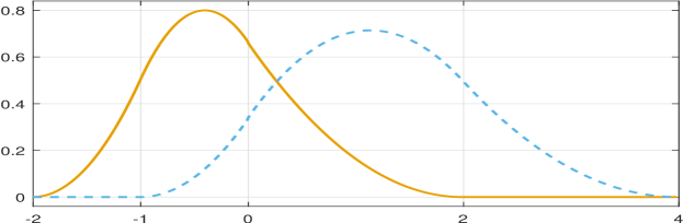
$\displaystyle n$	$\displaystyle r_{n}(\zeta_{-2})$	$\displaystyle r_{n}(\zeta_{-1})$
1	-0.9004	0.8333
2	-0.0362	0.5235
3	0.6611	0.9355
4	1.0683	1.2308
5	1.3178	1.4250

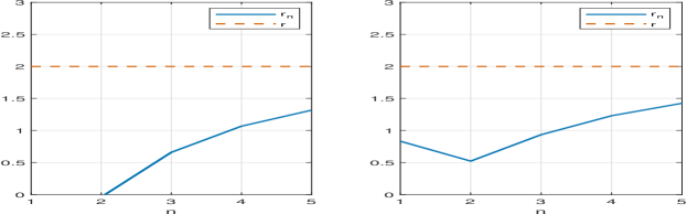
$\displaystyle n$	$\displaystyle r^{*}_{n}(\zeta_{k_{\ell}(\mathbf{Z})+1})$	$\displaystyle r^{*}_{n}(\zeta_{k_{\ell}(\mathbf{Z})+2})$
1	-0.9004	0.8333
2	0.8280	0.2136
3	2.0000	2.0001
4	2.0000	2.0000
5	2.0000	2.0000

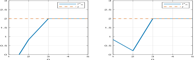
Figure 1: Semi-regular quadratic B-spline functions on the mesh $\displaystyle\bf{t}$ with $\displaystyle h_{\ell}=1$ and $\displaystyle h_{r}=2$ analyzed with the semi-regular Dubuc-Deslauriers $\displaystyle 6$-point tight wavelet frame. Top row: part of the subdivision matrix $\displaystyle\mathbf{Z}$ that corresponds to the non-shift-invariant refinable functions around $\displaystyle 0$ and the graphs of these functions $\displaystyle\zeta_{-2}$ and $\displaystyle\zeta_{-1}$. Middle row: estimates of the optimal Hölder-Zygmund exponents of $\displaystyle\zeta_{-2}$ and $\displaystyle\zeta_{-1}$ via linear regression (on the left) via the method in Proposition 4.10 (on the right). Bottom row: graphs of the estimates of the Hölder-Zygmund exponents.

On Figure 1 we give the estimates of the optimal Hölder-Zygmund exponents by both the linear regression method and by the method in Proposition 4.10. For the analysis we used the semi-regular tight wavelet frame constructed from the limits of the semi-regular Dubuc-Deslauriers $\displaystyle 6$-point subdivision scheme. This toy example already illustrates that the method proposed in Proposition 4.10 reaches the optimal exponent in few steps, while the linear regression method converges much slower.

4.3.2 Dubuc-Deslauriers $\displaystyle 4$-point scheme

In [29], the subdivision matrix $\displaystyle\mathbf{Z}$ of the semi-regular Dubuc-Deslauriers $\displaystyle 4$-point scheme is obtained by requiring that $\displaystyle\mathbf{Z}$ is $\displaystyle 2$-slanted, has at most $\displaystyle 7$ non-zero entries in each column and $\displaystyle\mathbf{Z}(2i,k)=\delta_{i,k}$, $\displaystyle i,\;k\in\mathbb{Z}$, $\displaystyle\mathbf{Z}\;\mathbf{t}^{\alpha}\;=\;(\mathbf{t}/2)^{\alpha}$ for $\displaystyle\alpha\in\{0,\dots,3\}$ with $\displaystyle\mathbf{t}$ in (1). In this case, there are $\displaystyle 5$ irregular (non-shift-invariant) refinable functions depicted on Figure 2. Due to results in [12], it is well known that the optimal exponent of all these irregular functions is equal to $\displaystyle 2$. Again, the method in Proposition 4.10 remarkably outperforms the linear regression method.

$\displaystyle\mathbf{Z}(-9:9,-3:3)\;=\;$

$$\begin{bmatrix}-1/16\\ 0\\ 9/16&-1/16\\ 1&0\\ 9/16&9/16&-1/16\\ 0&1&0\\ -1/16&9/16&9/16&-1/16\\ &0&1&0\\ &-5/64&5/8&15/32&-1/64\\ &&0&1&0\\ &&-1/5&3/4&1/2&-1/20\\ &&&0&1&0\\ &&&-1/16&9/16&9/16&-1/16\\ &&&&0&1&0\\ &&&&-1/16&9/16&9/16\\ &&&&&0&1\\ &&&&&-1/16&9/16\\ &&&&&&0\\ &&&&&&-1/16\end{bmatrix}$$

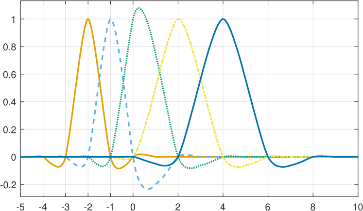
$\displaystyle n$	$\displaystyle r_{n}(\zeta_{-2})$	$\displaystyle r_{n}(\zeta_{-1})$	$\displaystyle r_{n}(\zeta_{0})$	$\displaystyle r_{n}(\zeta_{1})$	$\displaystyle r_{n}(\zeta_{2})$
1	-0.0589	-0.6276	-0.4561	-0.6674	1.4706
2	1.5123	0.4586	0.6302	0.8716	1.8356
3	1.8333	1.0375	1.1799	1.5818	2.2240
4	1.9052	1.3336	1.4487	1.8532	2.3523
5	1.9360	1.5117	1.6052	1.9587	2.3596
6	1.9516	1.6266	1.7032	2.0022	2.3239
7	1.9615	1.7052	1.7688	2.0209	2.2820
8	1.9683	1.7614	1.8148	2.0286	2.2436
9	1.9734	1.8030	1.8484	2.0310	2.2108
10	1.9774	1.8346	1.8736	2.0310	2.1833
11	1.9805	1.8592	1.8929	2.0298	2.1604
12	1.9830	1.8786	1.9082	2.0281	2.1413
13	1.9851	1.8944	1.9204	2.0262	2.1252
14	1.9868	1.9072	1.9303	2.0244	2.1116
15	1.9882	1.9179	1.9385	2.0226	2.1001
16	1.9895	1.9268	1.9453	2.0209	2.0902

$\displaystyle n$	$\displaystyle r^{*}_{n}(\zeta_{-2})$	$\displaystyle r^{*}_{n}(\zeta_{-1})$	$\displaystyle r^{*}_{n}(\zeta_{0})$	$\displaystyle r^{*}_{n}(\zeta_{1})$	$\displaystyle r^{*}_{n}(\zeta_{2})$
1	-0.0589	-0.6276	-0.4561	-0.6674	1.4706
2	3.0835	1.5448	1.7165	2.4105	2.2007
3	2.0585	2.0261	2.1006	2.7262	3.0086
4	1.8721	1.9392	1.9742	2.2284	2.4769
5	1.9764	1.9883	2.0064	2.0489	2.1474
6	1.9792	1.9897	1.9984	2.0131	2.0013
7	1.9920	1.9960	2.0004	2.0096	1.9997
8	1.9954	1.9977	1.9999	2.0041	2.0001
9	1.9979	1.9989	2.0000	2.0022	2.0000
10	1.9989	1.9995	2.0000	2.0011	2.0000
11	1.9995	1.9997	2.0000	2.0005	2.0000
12	1.9997	1.9999	2.0000	2.0003	2.0000
13	1.9999	1.9999	2.0000	2.0001	2.0000
14	1.9999	2.0000	2.0000	2.0001	2.0000
15	2.0000	2.0000	2.0000	2.0000	2.0000
16	2.0000	2.0000	2.0000	2.0000	2.0000

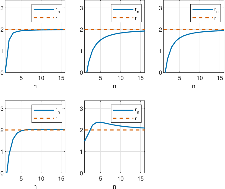
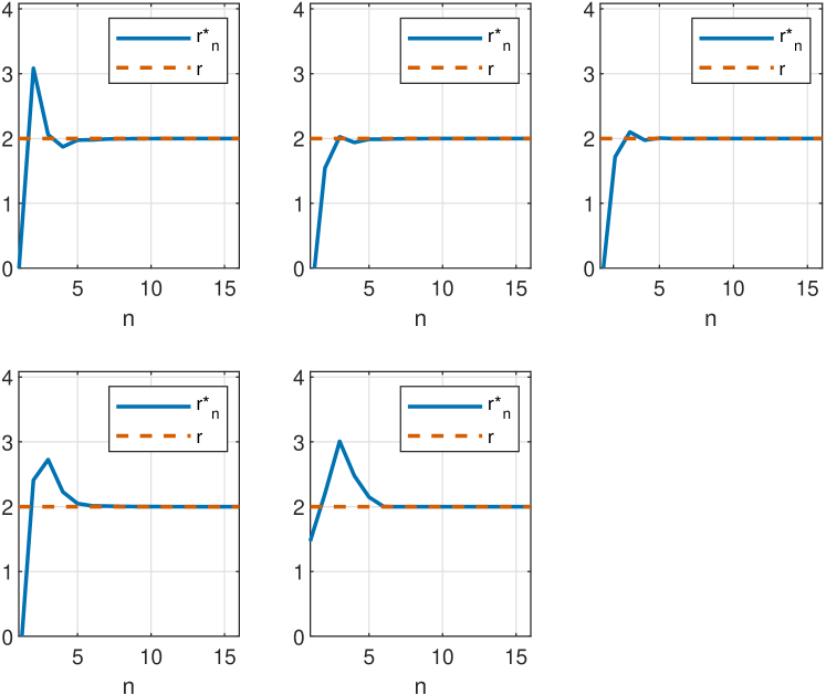
Figure 2: Semi-regular Dubuc-Deslauriers $\displaystyle 4$-point limit functions on the mesh $\displaystyle\bf{t}$ with $\displaystyle h_{\ell}=1$ and $\displaystyle h_{r}=2$ analyzed via the semi-regular Dubuc-Deslauriers $\displaystyle 6$-point tight wavelet frame. Top row: part of the subdivision matrix $\displaystyle\mathbf{Z}$ that corresponds to the non-shift-invariant refinable functions around $\displaystyle 0$ and the graphs of these functions $\displaystyle\zeta_{-2},\dots,\zeta_{2}$. Middle row: estimates of the optimal Hölder-Zygmund exponents of $\displaystyle\zeta_{-2},\dots,\zeta_{2}$ via linear regression (on the left) via the method in Proposition 4.10 (on the right). Bottom row: graphs of the estimates of the Hölder-Zygmund exponents.

4.3.3 Radial basis functions based interpolatory schemes

Using techniques similar to [28, 30], we extend the subdivision schemes [19, 20] based on radial basis functions to the semi-regular setting. Let $\displaystyle L\in\mathbb{N}$. We require that the subdivision matrix $\displaystyle\mathbf{Z}$ satisfies $\displaystyle\mathbf{Z}(2i,k)=\delta_{i,k}$ for $\displaystyle i,k\in\mathbb{Z}$. To determine the other entries of the $\displaystyle 2$-slanted matrix $\displaystyle\mathbf{Z}$ whose columns are centered at $\displaystyle\mathbf{Z}(2k,k)$, $\displaystyle k\in\mathbb{Z}$ and have support length at most $\displaystyle 4L-1$, we proceed as follows. We first choose a radial basis function $\displaystyle g(x)=g(|x|)$, $\displaystyle x\in\mathbb{R}$, which is conditionally positive definite of order $\displaystyle\eta\in\mathbb{N}$, i.e., for every set of pairwise distinct points $\displaystyle\{x_{i}\}_{i=1}^{N}\subset\mathbb{R}$ and coefficients $\displaystyle\{c_{i}\}_{i=1}^{N}\subset\mathbb{R}$, $\displaystyle N\in\mathbb{N}$, there exists a polynomial $\displaystyle\pi$ of degree at most $\displaystyle\eta-1$ such that

$$\sum_{i=1}^{N}\;c_{i}\;\pi(x_{i})\;=\;0$$

and the function $\displaystyle g$ satisfies

$$\sum_{i=1}^{N}\;\sum_{k=1}^{N}\;c_{i}\;c_{k}\;g(x_{i}-x_{k})\;\geq\;0.$$

The next step is to choose the order $\displaystyle m\in\{\eta,\dots,2L\}$ of polynomial reproduction and, for every set of $\displaystyle 2L$ consecutive points $\displaystyle\mathbf{t}(k-L+1),\;\dots,\;\mathbf{t}(k+L)$, $\displaystyle k\in\mathbb{Z}$, of the mesh $\displaystyle\mathbf{t}$ in (1), solve the linear system of equations

$$\begin{bmatrix}\mathbf{A}&\mathbf{B}\\ \\ \mathbf{B}^{T}&\mathbf{0}\end{bmatrix}\;\begin{bmatrix}\mathbf{u}\\ \\ \mathbf{v}\end{bmatrix}\;=\;\begin{bmatrix}\mathbf{r}\\ \\ \mathbf{s}\end{bmatrix}$$ (33)

with

$$\{\;\mathbf{A}(i,j)\;=\;g(\mathbf{t}(k-L+i)-\mathbf{t}(k-L+j))\;\}_{i,j=1,\dots,2L},\quad\{\;\mathbf{B}(i,j)\;=\;\mathbf{t}(k-L+i)^{j-1}\;\}_{i=1,\dots,2L,\;j=1,\dots,m},$$

$$\{\;\mathbf{r}(i)\;=\;g(x_{k}-\mathbf{t}(k-L+i))\;\}_{i=1,\dots,2L},\quad\{\;\mathbf{s}(j)\;=\;x_{k}^{j-1}\;\}_{j=1,\dots,m}\quad\hbox{and}$$

$$x_{k}\;=\;(\;\mathbf{t}(k)+\mathbf{t}(k+1)\;)/2.$$

Lastly, the vector $\displaystyle\mathbf{u}$ contains the entries of the $\displaystyle 2k+1$-th row of $\displaystyle\mathbf{Z}$ associated to the columns $\displaystyle k-L+1$ to $\displaystyle k+L$.

Remark 4.13.

$\displaystyle(i)$ Determining the rows of $\displaystyle\mathbf{Z}$ by solving the linear systems (33) for $\displaystyle k\in\mathbb{Z}$ guarantees the polynomial reproduction of degree at most $\displaystyle m-1$. Indeed, the condition $\displaystyle\mathbf{B}^{T}\;\mathbf{u}\;=\;\mathbf{s}$ forces $\displaystyle\mathbf{Z}$ to map samples over $\displaystyle\mathbf{t}$ of a polynomial of degree at most $\displaystyle m-1$ onto sample over the finer knots $\displaystyle\mathbf{t}/2$ of the same polynomial.

$\displaystyle(ii)$ If $\displaystyle m=2L$, the system of equations $\displaystyle\mathbf{B}^{T}\;\mathbf{u}\;=\;\mathbf{s}$ coincides with the one defining the Dubuc-Deslauriers $\displaystyle 2L$-point scheme in [28]. In this case, the system $\displaystyle\mathbf{B}^{T}\;\mathbf{u}\;=\;\mathbf{s}$ has a unique solution, which makes the presence of $\displaystyle\mathbf{A}$, i.e. of the radial basis function $\displaystyle g$ obsolete.

$\displaystyle(iii)$ If $\displaystyle m<2L$, the structure of the irregular limit functions around $\displaystyle 0$ reflect the transition (blending) between the two (one on the left and one on the right of $\displaystyle 0$) subdivision schemes of different regularity, see Example 4.1. This depends on the properties of the chosen underlying radial basic function $\displaystyle g$. For example, the blending produces no visible effect if $\displaystyle g$ is homogeneous, i.e. $\displaystyle g(\lambda x)=|\lambda|g(x)$, $\displaystyle\lambda\in\mathbb{R}$. In this case, for $\displaystyle\lambda>0$, the linear system of equations

$$\begin{bmatrix}\lambda\mathbf{I}&\mathbf{0}\\ \\ \mathbf{0}&\mathbf{L}\end{bmatrix}\;\begin{bmatrix}\mathbf{A}&\mathbf{B}\\ \\ \mathbf{B}^{T}&\mathbf{0}\end{bmatrix}\;\begin{bmatrix}\mathbf{I}&\mathbf{0}\\ \\ \mathbf{0}&\mathbf{L}/\lambda\end{bmatrix}\;\begin{bmatrix}\mathbf{I}&\mathbf{0}\\ \\ \mathbf{0}&\lambda\mathbf{L}^{-1}\end{bmatrix}\;\begin{bmatrix}\mathbf{u}\\ \\ \mathbf{v}\end{bmatrix}\;=\;\begin{bmatrix}\lambda\mathbf{I}&\mathbf{0}\\ \\ \mathbf{0}&\mathbf{L}\end{bmatrix}\;\begin{bmatrix}\mathbf{r}\\ \\ \mathbf{s}\end{bmatrix}$$ (34)

with the identity matrix $\displaystyle\mathbf{I}$ and $\displaystyle\mathbf{L}=\mathop{\mathrm{diag}}([\lambda^{j-1}]_{j=1,\dots,m})$ is equivalent to the system in (33) for the mesh $\displaystyle\lambda\mathbf{t}$. The structure of the linear system in (34) implies that $\displaystyle\mathbf{u}$ is the same as the one determined by (33).

$\displaystyle(iv)$ The argument in $\displaystyle(iii)$ with $\displaystyle\mathbf{L}=\mathbf{I}$ shows that the subdivision matrix obtained this way does not depend on the normalization of the radial basis function $\displaystyle g$, i.e. all functions $\displaystyle\lambda g$, $\displaystyle\lambda>0$, lead to the same subdivision scheme.

Example 4.1.

We consider the radial basis function introduced by M. Buhmann in [4]

$$g(x)\;=\;\left\{\begin{array}[]{rl}12x^{4}\log|x|\;-\;21x^{4}\;+\;32|x|^{3}\;-\;12x^{2}\;+\;1,&\textrm{ if }|x|<1,\\ \\ 0,&\textrm{ otherwise},\end{array}\right.$$ (35)

and choose $\displaystyle L=2$ and $\displaystyle m=1$. The resulting irregular functions $\displaystyle\zeta_{-2},\dots,\zeta_{2}$ are shown on Figure 3. The structure of $\displaystyle\zeta_{0}$ illustrates the blending effect (described in Remark 4.13 part $\displaystyle(iii)$) of two different subdivision schemes meeting at $\displaystyle 0$. Figure 3 also presents the estimates of the optimal Hölder-Zygmund exponents of $\displaystyle\zeta_{-2},\dots,\zeta_{2}$. These exponents are determined using the tight wavelet frame [28] based on the Dubuc-Deslauriers $\displaystyle 4$-point subdivision scheme. We again observe the phenomenon that the method in Proposition 4.10 converges faster than the linear regression.

$\displaystyle\mathbf{Z}(-9:9,-3:3)\;=\;$

$$\left[\begin{array}[]{ccccccc}0.1662&&&&&\\ 0&&&&&\\ 0.3338&0.1662&&&&&\\ 1&0&&&&&\\ 0.3338&0.3338&0.1662&&&&\\ 0&1&0&&&&\\ 0.1662&0.3338&0.3338&0.1662&&&\\ &0&1&0&&&\\ &0.1662&0.3338&0.3338&0.1662&&\\ &&0&1&0&&\\ &&0.2500&0.2500&0.2500&0.2500&\\ &&&0&1&0&\\ &&&0.2500&0.2500&0.2500&0.2500\\ &&&&0&1&0\\ &&&&0.2500&0.2500&0.2500\\ &&&&&0&1\\ &&&&&0.2500&0.2500\\ &&&&&&0\\ &&&&&&0.2500\\ \end{array}\right].$$

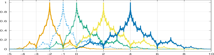
$\displaystyle n$	$\displaystyle r_{n}(\zeta_{-2})$	$\displaystyle r_{n}(\zeta_{-1})$	$\displaystyle r_{n}(\zeta_{0})$	$\displaystyle r_{n}(\zeta_{1})$	$\displaystyle r_{n}(\zeta_{2})$
1	2.3107	0.0955	-0.3137	1.9167	1.1751
2	1.3713	0.7568	0.1025	1.2398	0.7305
3	1.0062	0.5966	0.2212	0.9391	0.5609
4	0.8229	0.5853	0.2821	0.7386	0.4754
5	0.7185	0.5437	0.3146	0.6290	0.4269
6	0.6532	0.5226	0.3342	0.5552	0.3965
7	0.6097	0.5014	0.3466	0.5037	0.3763
8	0.5793	0.4860	0.3550	0.4664	0.3622
9	0.5571	0.4726	0.3608	0.4387	0.3519
10	0.5405	0.4618	0.3650	0.4175	0.3442
11	0.5278	0.4525	0.3681	0.4010	0.3383
12	0.5177	0.4448	0.3705	0.3879	0.3336
13	0.5097	0.4382	0.3723	0.3773	0.3299
14	0.5032	0.4325	0.3737	0.3686	0.3269
15	0.4978	0.4276	0.3749	0.3614	0.3244
16	0.4934	0.4234	0.3758	0.3554	0.3223

$\displaystyle n$	$\displaystyle r^{*}_{n}(\zeta_{-2})$	$\displaystyle r^{*}_{n}(\zeta_{-1})$	$\displaystyle r^{*}_{n}(\zeta_{0})$	$\displaystyle r^{*}_{n}(\zeta_{1})$	$\displaystyle r^{*}_{n}(\zeta_{2})$
1	2.3107	0.0955	-0.3137	1.9167	1.1751
2	0.4319	1.4181	0.5186	0.5630	0.2859
3	0.4673	0.0025	0.3595	0.4631	0.3133
4	0.4549	0.7000	0.4071	0.2370	0.3029
5	0.4585	0.3168	0.3879	0.3727	0.3069
6	0.4573	0.4855	0.3888	0.3053	0.3053
7	0.4577	0.3743	0.3860	0.3059	0.3059
8	0.4576	0.4187	0.3846	0.3057	0.3057
9	0.4576	0.3832	0.3839	0.3058	0.3058
10	0.4576	0.3957	0.3831	0.3057	0.3057
11	0.4576	0.3838	0.3829	0.3058	0.3058
12	0.4576	0.3872	0.3825	0.3058	0.3058
13	0.4576	0.3832	0.3824	0.3058	0.3058
14	0.4576	0.3841	0.3823	0.3058	0.3058
15	0.4576	0.3827	0.3822	0.3058	0.3058
16	0.4576	0.3829	0.3822	0.3058	0.3058

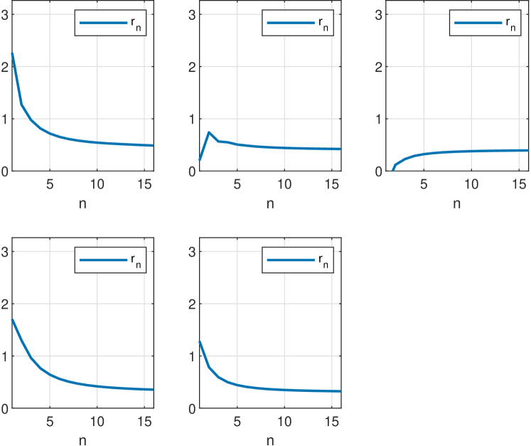
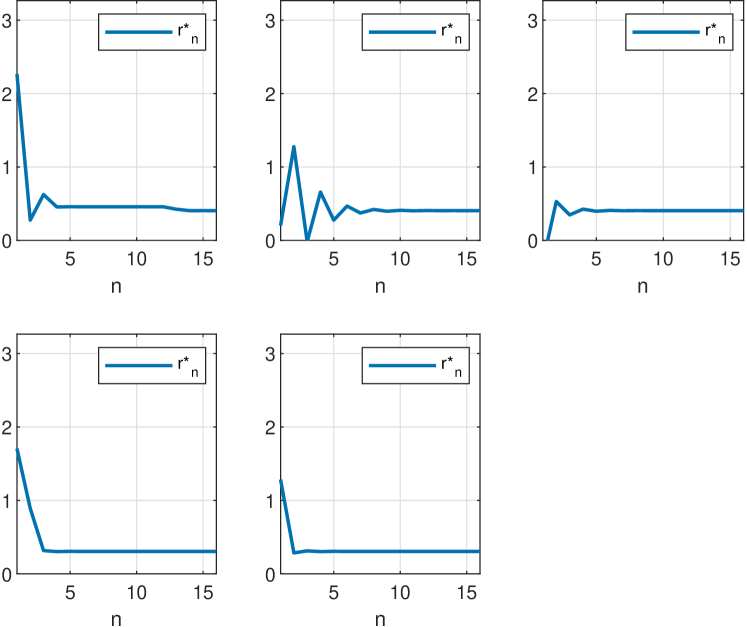
Figure 3: Semi-regular interpolatory subdivision scheme based on $\displaystyle g$ in (35), $\displaystyle L=2$, $\displaystyle m=1$, on the mesh $\displaystyle\bf{t}$ with $\displaystyle h_{\ell}=1$ and $\displaystyle h_{r}=2$ analyzed via the semi-regular Dubuc-Deslauriers $\displaystyle 4$-point tight wavelet frame. Top row: part of the subdivision matrix $\displaystyle\mathbf{Z}$ that corresponds to the non-shift-invariant refinable functions around $\displaystyle 0$ and the graphs of these functions $\displaystyle\zeta_{-2},\dots,\zeta_{2}$. Middle row: estimates of the optimal Hölder-Zygmund exponents of $\displaystyle\zeta_{-2},\dots,\zeta_{2}$ via linear regression (on the left) via the method in Proposition 4.10 (on the right). Bottom row: graphs of the estimates of the Hölder-Zygmund exponents.

Example 4.2.

Another radial basis function that we consider is the polyharmonic function $\displaystyle g(x)\;=\;|x|$, $\displaystyle x\in\mathbb{R}$. The corresponding irregular part of the interpolatory subdivision matrix $\displaystyle\mathbf{Z}$ is determined for $\displaystyle L=2$ and $\displaystyle m=3$, see Figure 4. Note that the regular part of the subdivision matrix $\displaystyle\mathbf{Z}$ (see the first and the last columns corresponding to the regular parts of the mesh) coincides with the subdivision matrix of the regular Dubuc-Deslauriers $\displaystyle 4$-point scheme. Due to the observation in Remark 4.13 part $\displaystyle(iii)$, the absence of the blending effect is due to our choice of a homogeneous function $\displaystyle g$. We would like to emphasise that the resulting subdivision scheme around $\displaystyle 0$ is not the semi-regular Dubuc-Deslauriers $\displaystyle 4$-point scheme, compare with Figure 2. Indeed, the polynomial reproduction around $\displaystyle 0$ is of one degree lower. We also lose regularity (the Dubuc-Deslauriers $\displaystyle 4$-point scheme is $\displaystyle C^{2-\epsilon}$, $\displaystyle\epsilon>0$) but overall the irregular limit functions on Figure 4 have a more uniform behavior than those on Figure 2. We again observe that the method in Proposition 4.10 yields better estimates for the optimal Hölder-Zygmund exponent, see tables on Figure 4.

$\displaystyle\mathbf{Z}(-9:9,-3:3)\;=\;$

$$\left[\begin{array}[]{ccccccc}-1/16\\ 0\\ 9/16&-1/16\\ 1&0\\ 9/16&9/16&-1/16\\ 0&1&0\\ -1/16&9/16&9/16&-1/16\\ &0&1&0\\ &-1/24&19/36&13/24&-1/36&\\ &&0&1&0\\ &&-1/9&7/12&11/18&-1/12\\ &&&0&1&0\\ &&&-1/16&9/16&9/16&-1/16\\ &&&&0&1&0\\ &&&&-1/16&9/16&9/16\\ &&&&&0&1\\ &&&&&-1/16&9/16\\ &&&&&&0\\ &&&&&&-1/16\end{array}\right].$$

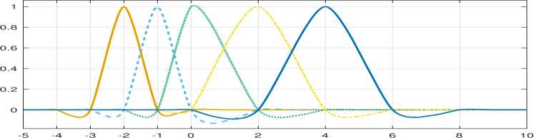
$\displaystyle n$	$\displaystyle r_{n}(\zeta_{-2})$	$\displaystyle r_{n}(\zeta_{-1})$	$\displaystyle r_{n}(\zeta_{0})$	$\displaystyle r_{n}(\zeta_{1})$	$\displaystyle r_{n}(\zeta_{2})$
1	-0.0163	-0.5174	-0.3984	-0.5637	1.4525
2	1.8110	0.6301	0.2509	0.5646	1.5324
3	2.3259	0.9516	0.7115	1.0643	1.6848
4	2.1635	1.1421	1.0006	1.3048	1.7340
5	2.0346	1.2779	1.1895	1.4400	1.7552
6	1.9538	1.3766	1.3178	1.5230	1.7640
7	1.9029	1.4495	1.4081	1.5777	1.7677
8	1.8695	1.5043	1.4740	1.6155	1.7692
9	1.8466	1.5463	1.5232	1.6429	1.7696
10	1.8303	1.5791	1.5610	1.6633	1.7695
11	1.8183	1.6050	1.5906	1.6789	1.7693
12	1.8092	1.6260	1.6141	1.6911	1.7689
13	1.8022	1.6430	1.6332	1.7008	1.7685
14	1.7967	1.6571	1.6488	1.7087	1.7681
15	1.7922	1.6689	1.6618	1.7152	1.7677
16	1.7886	1.6788	1.6727	1.7206	1.7674

$\displaystyle n$	$\displaystyle r^{*}_{n}(\zeta_{-2})$	$\displaystyle r^{*}_{n}(\zeta_{-1})$	$\displaystyle r^{*}_{n}(\zeta_{0})$	$\displaystyle r^{*}_{n}(\zeta_{1})$	$\displaystyle r^{*}_{n}(\zeta_{2})$
1	-0.0163	-0.5174	-0.3984	-0.5637	1.4525
2	3.6383	1.7777	0.9002	1.6929	1.6124
3	2.9182	1.3190	1.5699	1.8541	2.0135
4	0.9991	1.5830	1.6965	1.7672	1.7787
5	1.5859	1.7110	1.7445	1.7700	1.7838
6	1.7105	1.7467	1.7568	1.7642	1.7665
7	1.7468	1.7580	1.7612	1.7638	1.7649
8	1.7580	1.7615	1.7625	1.7633	1.7636
9	1.7615	1.7626	1.7630	1.7632	1.7633
10	1.7626	1.7630	1.7631	1.7632	1.7632
11	1.7630	1.7631	1.7632	1.7632	1.7632
12	1.7631	1.7632	1.7632	1.7632	1.7632
13	1.7632	1.7632	1.7632	1.7632	1.7632
14	1.7632	1.7632	1.7632	1.7632	1.7632
15	1.7632	1.7632	1.7632	1.7632	1.7632
16	1.7632	1.7632	1.7632	1.7632	1.7632

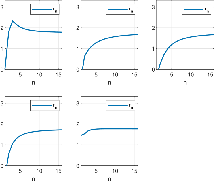
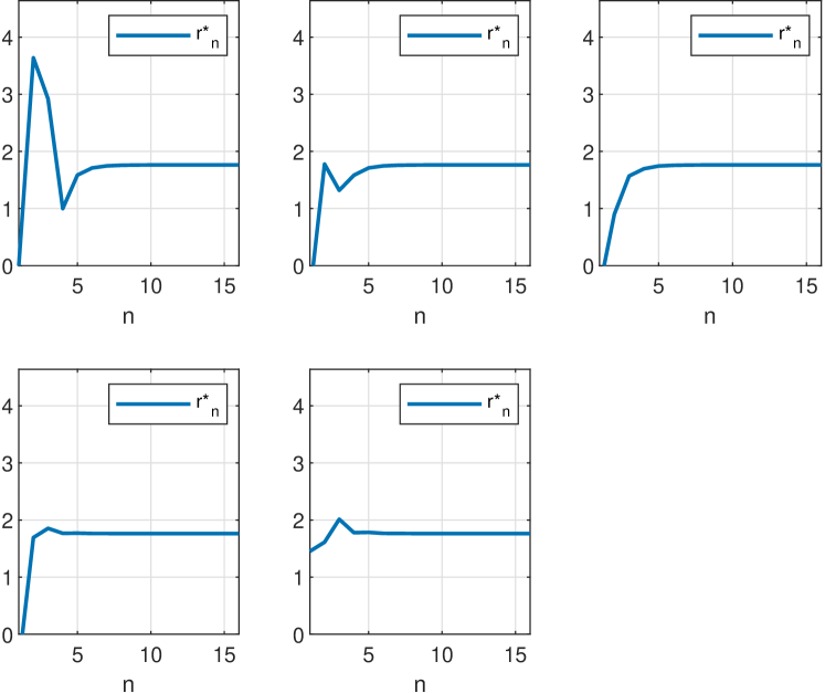
Figure 4: Semi-regular interpolatory scheme based on the polyharmonic function $\displaystyle g(x)=|x|$, $\displaystyle L=2$ and $\displaystyle m=3$ on the mesh $\displaystyle\bf{t}$ with $\displaystyle h_{\ell}=1$, $\displaystyle h_{r}=2$ analyzed with the semi-regular Dubuc-Deslauriers $\displaystyle 6$-point scheme. Top row: part of the subdivision matrix $\displaystyle\mathbf{Z}$ that corresponds to the non-shift-invariant refinable functions around $\displaystyle 0$ and the graphs of these functions $\displaystyle\zeta_{-2},\dots,\zeta_{2}$. Middle row: estimates of the optimal Hölder-Zygmund exponents of $\displaystyle\zeta_{-2},\dots,\zeta_{2}$ via linear regression (on the left) via the method in Proposition 4.10 (on the right). Bottom row: graphs of the estimates of the Hölder-Zygmund exponents.

Similar results, enlightening the viability of our method, appear for a large number of other members of the semi-regular families of subdivision schemes (i.e. B-splines, Dubuc-Deslauriers and interpolatory schemes based on (inverse) multi-quadrics, gaussians, Wendland’s functions, Wu’s functions, Buhmann’s functions, polyharmonic functions and Euclid’s hat functions [14]). For the interested reader, a MATLAB function for the generation of semi-regular RBFs-based interpolatory schemes is available at [27].

Acknowledgements: The authors thank Karlheinz Gröchenig for his fruitful suggestions and the Erwin Schrödinger International Institute for Mathematics and Physics (ESI), Vienna, Austria, for discussion stimulating environment. Maria Charina is sponsored by the Austrian Science Foundation (FWF) grant P28287-N35. Costanza Conti, Lucia Romani and Alberto Viscardi have conducted this research within Research ITalian network on Approximation (RITA).

References

References

- [1] C. Beccari, G. Casciola, and L. Romani, Polynomial-based non-uniform interpolatory subdivision with features control, J. Comput. Appl. Math., 235 (2011), pp. 4754–4769.
- [2] C. V. Beccari, G. Casciola, and L. Romani, Non-uniform interpolatory curve subdivision with edge parameters built upon compactly supported fundamental splines, BIT, 51 (2011), pp. 781–808.
- [3] L. Borup, R. Gribonval, and M. Nielsen, Tight wavelet frames in Lebesgue and Sobolev spaces, J. Funct. Spaces Appl., 2 (2004), pp. 227–252.
- [4] M. D. Buhmann, Radial basis functions, in Acta numerica, 2000, vol. 9 of Acta Numer., Cambridge Univ. Press, Cambridge, 2000, pp. 1–38.
- [5] O. Christensen, An introduction to frames and Riesz bases, Applied and Numerical Harmonic Analysis, Birkhäuser/Springer, [Cham], second ed., 2016.
- [6] C. Chui and J. de Villiers, Wavelet subdivision methods, CRC Press, Boca Raton, FL, 2011. GEMS for rendering curves and surfaces, With a foreword by Tom Lyche.
- [7] C. K. Chui, An introduction to wavelets, vol. 1 of Wavelet Analysis and its Applications, Academic Press, Inc., Boston, MA, 1992.
- [8] C. K. Chui, W. He, and J. Stöckler, Nonstationary tight wavelet frames. I. Bounded intervals, Appl. Comput. Harmon. Anal., 17 (2004), pp. 141–197.
- [9] , Nonstationary tight wavelet frames. II. Unbounded intervals, Appl. Comput. Harmon. Anal., 18 (2005), pp. 25–66.
- [10] E. Cordero and K. Gröchenig, Localization of frames. II, Appl. Comput. Harmon. Anal., 17 (2004), pp. 29–47.
- [11] I. Daubechies, Ten lectures on wavelets, vol. 61 of CBMS-NSF Regional Conference Series in Applied Mathematics, Society for Industrial and Applied Mathematics (SIAM), Philadelphia, PA, 1992.
- [12] I. Daubechies, I. Guskov, and W. Sweldens, Regularity of irregular subdivision, Constr. Approx., 15 (1999), pp. 381–426.
- [13] G. Deslauriers and S. Dubuc, Symmetric iterative interpolation processes, Constr. Approx., 5 (1989), pp. 49–68. Fractal approximation.
- [14] G. E. Fasshauer, Meshfree approximation methods with MATLAB, vol. 6 of Interdisciplinary Mathematical Sciences, World Scientific Publishing Co. Pte. Ltd., Hackensack, NJ, 2007. With 1 CD-ROM (Windows, Macintosh and UNIX).
- [15] M. Frazier and B. Jawerth, Decomposition of Besov spaces, Indiana Univ. Math. J., 34 (1985), pp. 777–799.
- [16] B. Han and Z. Shen, Characterization of Sobolev spaces of arbitrary smoothness using nonstationary tight wavelet frames, Israel J. Math., 172 (2009), pp. 371–398.
- [17] M. Holschneider and P. Tchamitchian, Régularite locale de la fonction “non-différentiable” de Riemann, in Les ondelettes en 1989 (Orsay, 1989), vol. 1438 of Lecture Notes in Math., Springer, Berlin, 1990, pp. 102–124, 209–210.
- [18] A. Kunoth, On the fast evaluation of integrals of refinable functions, in Wavelets, images, and surface fitting (Chamonix-Mont-Blanc, 1993), A K Peters, Wellesley, MA, 1994, pp. 327–334.
- [19] B.-G. Lee, Y. J. Lee, and J. Yoon, Stationary binary subdivision schemes using radial basis function interpolation, Adv. Comput. Math., 25 (2006), pp. 57–72.
- [20] Y. J. Lee and J. Yoon, Analysis of stationary subdivision schemes for curve design based on radial basis function interpolation, Appl. Math. Comput., 215 (2010), pp. 3851–3859.
- [21] P. G. Lemarié and Y. Meyer, Ondelettes et bases hilbertiennes, Rev. Mat. Iberoamericana, 2 (1986), pp. 1–18.
- [22] J. M. Lounsbery, Multiresolution analysis for surfaces of arbitrary topological type, ProQuest LLC, Ann Arbor, MI, 1994. Thesis (Ph.D.)–University of Washington.
- [23] Y. Meyer, Wavelets and operators, vol. 37 of Cambridge Studies in Advanced Mathematics, Cambridge University Press, Cambridge, 1992. Translated from the 1990 French original by D. H. Salinger.
- [24] J. Peters and U. Reif, Subdivision surfaces, vol. 3 of Geometry and Computing, Springer-Verlag, Berlin, 2008. With introductory contributions by Nira Dyn and Malcolm Sabin.
- [25] S. Pilipović, D. s. Rakić, and J. Vindas, New classes of weighted Hölder-Zygmund spaces and the wavelet transform, J. Funct. Spaces Appl., (2012), pp. Art. ID 815475, 18.
- [26] L. F. Villemoes, Wavelet analysis of refinement equations, SIAM J. Math. Anal., 25 (1994), pp. 1433–1460.
- [27] A. Viscardi, Semi-regular interpolatory rbf-based subdivision schemes. Mendeley Data, 2018.
- [28] , Semi-regular Dubuc-Deslauriers wavelet tight frames, J. Comput. Appl. Math., (submitted).
- [29] J. Warren, Binary subdivision schemes for functions over irregular knot sequences, in Mathematical methods for curves and surfaces (Ulvik, 1994), Vanderbilt Univ. Press, Nashville, TN, 1995, pp. 543–562.
- [30] J. Warren and H. Weimer, Subdivision Methods for Geometric Design: A Constructive Approach, Morgan Kaufmann Publishers Inc., San Francisco, CA, USA, 1st ed., 2001.