Eigenvalues of the Laplacian on the Goldberg-Coxeter constructions for $3$- and $4$-valent graphs

Abstract.

We are concerned with spectral problems of the Goldberg-Coxeter construction for $3$- and $4$-valent finite graphs. The Goldberg-Coxeter constructions $\operatorname{GC}_{k,l}(X)$ of a finite $3$- or $4$-valent graph $X$ are considered as “subdivisions” of $X$, whose number of vertices are increasing at order $O(k^{2}+l^{2})$, nevertheless which have bounded girth. It is shown that the first (resp. the last) $o(k^{2})$ eigenvalues of the combinatorial Laplacian on $\operatorname{GC}_{k,0}(X)$ tend to $0$ (resp. tend to $6$ or $8$ in the $3$- or $4$-valent case, respectively) as $k$ goes to infinity. A concrete estimate for the first several eigenvalues of $\operatorname{GC}_{k,l}(X)$ by those of $X$ is also obtained for general $k$ and $l$. It is also shown that the specific values always appear as eigenvalues of $\operatorname{GC}_{2k,0}(X)$ with large multiplicities almost independently to the structure of the initial $X$. In contrast, some dependency of the graph structure of $X$ on the multiplicity of the specific values is also studied.

1. Introduction

The Goldberg-Coxeter construction is a subdivision of a $3$- or $4$-valent graph, and it is defined by Dutour-Deza [5] for a plane graph based on a simplicial subdivision of regular polytopes in [1, 15]. In [5], it is pointed out that it often appears in chemistry and architecture, and its combinatorial and algebraic structures are investigated. Goldberg-Coxeter constructions of regular polyhedra generate a class of Archimedean polyhedra, and infinite sequence of polyhedra, which are called Goldberg polyhedra. For example a Goldberg-Coxeter construction of a dodecahedron generates a truncated-icosahedron, which is known as a fullerene $C_{60}$ [17, 24]. Goldberg-Coxeter constructions are also applied to Mackay-like crystals, and explain large scale of spatial fullerenes [21, 23]. Mathematical modeling of self-assembly in nature is also widely studied in [1, 18]. Recently, Fujita et al. have synthesized molecule structures with $4$-valent Goldberg polyhedra, and they explain self-assembly from viewpoints of chemistry and biology [13].

On the other hand, the stability of a molecule is explained by eigenvalues of the finite graphs which express the molecule structure by Hückel method [2]. Hence, studies for eigenvalues of Goldberg-Coxeter constructions are worth trying. DeVos, Goddyn, Mohar, and Šámal considered eigenvalues of $(3,6)$-fullerenes (cf.[4]). A $(3,6)$-fullerene $X$ is a $3$-valent plane graph whose faces are triangles and hexagons. We consider general $3$- or $4$-valent graphs, and if a graph is $(k,6)$-fullerene, then its Goldberg-Coxeter constructions are also $(k,6)$-fullerenes. The Goldberg-Coxeter construction $\operatorname{GC}_{k,l}(X)$ of a $3$- or $4$-valent graph $X$ has the parameters $k$ and $l$ both of which are integers and they are regarded to indicate a point in the triangular or square lattices, respectively. Then we are concerned with behavior of eigenvalues of $\operatorname{GC}_{k,l}(X)$ when $k$ and $l$ tend to infinity.

Throughout this paper, unless otherwise indicated, a graph is always assumed to be connected, finite and simple. For a graph $X$, let us denote by $V(X)$ the set of vertices of $X$, and by $E(X)$ the set of undirected edges of $X$. For $p\in V(X)$, the set of its neighboring vertices is denoted by $N_{X}(p)$. The combinatorial Laplacian $\Delta_{X}$, simply called the Laplacian, of a graph $X$ acts on the set $\mathbb{C}^{V(X)}$ of functions on $V(X)$ and is defined as

$$(\Delta_{X}f)(p):=\deg(p)f(p)-\sum_{q\in N_{X}(p)}f(q)\quad\text{for $f\in\mathbb{C}^{V(X)}$ and $p\in V(X)$},$$

where $\deg(p)$ denotes the degree of the vertex $p$. As is well-known, the eigenvalues of $\Delta_{X}$ for a regular graph $X$ of degree $r$ necessarily lie in the interval $[0,2r]$.

The definition of the Goldberg-Coxeter constructions extends for general $3$- or $4$-valent graph $X=(V(X),E(X))$ equipped with an orientation at each vertex, in the sense that, for each $p\in V(X)$, the set of edges emanating from $p$ is ordered. As shall be explained later (cf. Proposition 2.2), if, in particular, $X$ is “appropriately” embedded in an oriented surface, then $X$ is endowed with a natural orientation at each vertex and $\operatorname{GC}_{k,l}(X)$ remains to be also embedded in the same surface.

There is a long line of works on upper bounds for the (especially, first nonzero) eigenvalues of general planar or genus $g$ finite graphs (see [19, 25] and the references therein). In [20], it is proved that the $i$-th eigenvalue of a graph embedded in an oriented surface of genus $g$ is estimated from above by $O((g+1)\log^{2}(g+1)i/n)$, where $n$ is the number of the vertices. The following theorem does not only depend on the genus, but contains an assertion on the last several eigenvalues of $\operatorname{GC}_{k,0}(X)$.

Theorem 1.1.

Let $X=(V(X),E(X))$ be a connected, finite and simple $3$- or $4$-valent graph equipped with an orientation at each vertex, and $\operatorname{GC}_{k,0}(X)$ be the Goldberg-Coxeter construction of $X$ for $k\geq 1$. Then, for any number $o(k^{2})$ satisfying $o(k^{2})/k^{2}\to 0$ as $k\to\infty$, the first (resp. the last) $o(k^{2})$ eigenvalues of the Laplacian of $\operatorname{GC}_{k,0}(X)$ tend to $0$ (resp. tend to $6$ or $8$ in the $3$- or $4$-valent case, respectively) as $k$ goes to infinity.

Here we note that $\operatorname{GC}_{k,0}(X)$ has $k^{2}\lvert{V(X)}\rvert=O(k^{2})$ vertices and the above result is the best in matters of the convergence to $0$ or to the natural upper bound. As for the first and the last $\lvert{V(X)}\rvert$ eigenvalues, the following concrete estimates are also obtained.

Theorem 1.2.

Let $X=(V(X),E(X))$ be a connected, finite and simple $3$- or $4$-valent graph equipped with an orientation at each vertex, $X^{\prime}=\operatorname{GC}_{k,l}(X)$ be the Goldberg-Coxeter construction of $X$, where $k\geq l\geq 0$ and $k\neq 0$ and

$$0=\lambda_{1}(X)<\lambda_{2}(X)\leq\cdots\leq\lambda_{\lvert{V(X)}\rvert}(X),$$

$$0=\lambda_{1}(X^{\prime})<\lambda_{2}(X^{\prime})\leq\cdots\leq\lambda_{\lvert{V(X^{\prime})}\rvert}(X^{\prime})$$

be the eigenvalues of their Laplacians $\Delta_{X}$, $\Delta_{X^{\prime}}$, respectively. Then for $i=1,2,\dots,\lvert{V(X)}\rvert$,

(1.1) $$\lambda_{i}(\operatorname{GC}_{k,l}(X))\leq\left\{\begin{aligned} &\frac{3k}{k^{2}+kl+l^{2}}\lambda_{i}(X),&&\text{if $X$ is $3$-valent},\\ &\frac{2k}{k^{2}+l^{2}}\lambda_{i}(X),&&\text{if $X$ is $4$-valent}.\end{aligned}\right.$$

If in particular $X$ is a bipartite $3$-valent graph, then for $i=1,2,\dots,\lvert{V(X)}\rvert$,

(1.2) $$\lambda_{\lvert{V(\operatorname{GC}_{k,l}(X))}\rvert-i+1}(\operatorname{GC}_{k,l}(X))\geq 6-\frac{3k}{k^{2}+kl+l^{2}}\lambda_{i}(X).$$

In the case that $l=0$, the last $\lvert{V(X)}\rvert$ eigenvalues of $\operatorname{GC}_{k,0}(X)$ satisfy

(1.3) $$\lambda_{\lvert{V(\operatorname{GC}_{k,0}(X))}\rvert-i+1}(\operatorname{GC}_{k,0}(X))\geq\left\{\begin{aligned} &3+\sqrt{5+4\cos\frac{2\pi}{k}},&&\text{if $X$ is $3$-valent},\\ &4+4\cos\frac{2\pi}{k},&&\text{if $X$ is $4$-valent and $k$ is even},\\ &4+4\cos\frac{\pi}{k},&&\text{if $X$ is $4$-valent and $k$ is odd},\end{aligned}\right.$$

for $i=1,2,\dots,\lvert{V(X)}\rvert$.

Moreover we have the following result.

Theorem 1.3.

Let $X$ be a $3$-valent (resp. $4$-valent) graph satisfying the same assumptions as in Theorem 1.2. For any real number $\lambda\in[0,6]$ (resp. $\lambda\in[0,8]$), there exists a sequence $(\lambda_{k})_{k}$ of eigenvalues of $\operatorname{GC}_{k,0}(X)$ which converges to $\lambda$ as $k$ tends to infinity.

As the following theorems show the Goldberg-Coxeter constructions have also steady eigenvalues.

Theorem 1.4.

Let $X$ be a connected, finite and simple $3$-valent graph equipped with an orientation at each vertex, and $\operatorname{GC}_{2k,0}(X)$ be its Goldberg-Coxeter constructions for $k\in\mathbb{N}$.

1. $\operatorname{GC}_{2k,0}(X)$ has eigenvalue $4$, whose multiplicity is at least $\lceil k/2\rceil$.

2. $\operatorname{GC}_{2k,0}(X)$ has eigenvalue $2$, whose multiplicity is at least $\lfloor k/2\rfloor$.

In Theorem 1.4, $\lceil x\rceil$ (resp. $\lfloor x\rfloor$) denotes the smallest integer $\geq x$ (resp. the largest integer $\leq x$).

Theorem 1.5.

Let $X$ be a connected, finite and simple $4$-valent graph equipped with an orientation at each vertex, and $\operatorname{GC}_{2k,0}(X)$ be its Goldberg-Coxeter constructions for $k\in\mathbb{N}$. Then, for $k\geq 2$, $\operatorname{GC}_{2k,0}$ has eigenvalue $4$, whose multiplicity is at least $\lceil(k-1)/2\rceil$.

On the other hand, the multiplicities of eigenvalues $2$ and $4$ would depend on the graph structure of $X$ and the following is obtained.

Theorem 1.6.

Let $X$ be a connected, finite and simple $3$-valent graph which is embedded in a plane. Assume that the number of edges surrounding each face is divisible by $3$. Then the following hold.

1. The multiplicity of eigenvalue $4$ of $\operatorname{GC}_{2,0}(X)$ is at least $3$.

2. For any $k\in\mathbb{N}$, both $\operatorname{GC}_{k,0}(X)$ and $\operatorname{GC}_{k,k}(X)$ have eigenvalue $4$ (resp. $2$), whose multiplicity is at least $\lceil k/2\rceil$ (resp. $\lfloor k/2\rfloor$).

The result (1) of Theorem 1.6 is also obtained by observing that the $\operatorname{GC}_{2.0}(X)$ is a covering graph of the $K_{4}$ graph.

Examples of numerical computations of multiplicities of eigenvalues $2$ and $4$ are shown in Tables 1 and 2.

Table 1. The multiplicities of eigenvalue $4$ for $\operatorname{GC}_{k,0}(X)$ ($k=1,2,\ldots,10$)

X	$(1,0)$	$(2,0)$	$(3,0)$	$(4,0)$	$(5,0)$	$(6,0)$	$(7,0)$	$(8,0)$	$(9,0)$	$(10,0)$
tetrahedron	$3$	$6$	$9$	$12$	$15$	$18$	$21$	$24$	$27$	$30$
cube	$3$	$4$	$3$	$12$	$3$	$20$	$3$	$28$	$3$	$36$
dodecahedron	$0$	$6$	$0$	$18$	$0$	$30$	$0$	$42$	$0$	$54$
octahedron	$3$	$4$	$3$	$12$	$3$	$20$	$3$	$28$	$3$	$36$

Table 2. The multiplicities of eigenvalue $2$ for $\operatorname{GC}_{k,0}(X)$ ($k=1,2,\ldots,10$)

X	$(1,0)$	$(2,0)$	$(3,0)$	$(4,0)$	$(5,0)$	$(6,0)$	$(7,0)$	$(8,0)$	$(9,0)$	$(10,0)$
tetrahedron	$0$	$3$	$6$	$9$	$12$	$15$	$18$	$21$	$24$	$27$
cube	$3$	$4$	$3$	$12$	$3$	$20$	$3$	$28$	$3$	$36$
dodecahedron	$5$	$6$	$5$	$18$	$5$	$30$	$5$	$42$	$5$	$54$
octahedron	$0$	$0$	$1$	$1$	$0$	$1$	$0$	$1$	$1$	$0$

Problems on eigenvalues of combinatorial Laplacian on regular graphs are extensively investigated. In particular, an explicit formula of a limit density of eigenvalue distributions of certain sequences of regular graphs was obtained in [22], and its geometric proof using a trace formula is given in [16] (see also [3]). One of points in these works is that the sequence $\{X_{n}\}$ of $q$-regular graphs with number of vertices $\lvert{X_{n}}\rvert\to\infty$ as $n\to\infty$ is assumed to have large girths $g(X_{n})\to\infty$ as $n\to\infty$. From this assumption, the graphs $X_{n}$ get similar, as $n\to\infty$, to a universal covering graph, namely a $q$-regular tree at least locally, and then a trace formula becomes able to apply. The girths of the Goldberg-Coxeter constructions $\{\operatorname{GC}_{k,l}(X)\}_{k,l}$ with an initial graph $X$ are uniformly bounded with respect to the parameters $k$ and $l$, and hence it would not be so straightforward to apply a trace formula to obtain a limit distribution of the eigenvalue distributions.

This paper is organized as follows. In Section 2, after giving the precise definition of the Goldberg-Coxeter constructions $\operatorname{GC}_{k,l}(X)$, we study their structure which is related with the spectral problems. In particular, variants of coloring problems necessary for our purposes are collected in Subsection 2.2. Some of them might be obtained from well-known results. For example, readers are referred to the interesting papers [7, 8, 9, 10, 11, 12] due to Fisk where one can find a lot of results on various kinds of coloring problems. However, we think that there are no statements which are precisely the same and the proofs do not involve so much. Thus we decided to put their proofs here for completeness. In Section 3, we obtain two kinds of comparisons of the eigenvalues, one is that between the eigenvalues of $X$ and those of $\operatorname{GC}_{k,l}(X)$, and the other is that between the eigenvalues of the $(k,0)$-cluster and those of $\operatorname{GC}_{k,0}(X)$. In Section 4, all the eigenvalues of the $(k,0)$-cluster are found and the proofs of Theorems 1.1, 1.2 and 1.3 complete. In Section 5, we first present proofs of Theorem 1.4 and 1.5. At the end of this paper, we shall give a few criteria for a $3$-valent plane graph $X$ so that some $\operatorname{GC}_{k,0}(X)$’s have eigenvalues $2$ or $4$, which proves Theorem 1.6.

2. Goldberg-Coxeter constructions

This section studies the structure of Goldberg-Coxeter constructions, which shall be necessary in the subsequent sections.

The notion of Goldberg-Coxeter constructions is defined, due to Deza-Dutour [5, 6], for a plane graph. The definition can be extended for a nonplanar graph $X$; indeed, $X$ has only to be equipped with an “orientation at each vertex”, and if, in particular, $X$ is “appropriately” embedded on an oriented surface, then the constructions can be done on the surface (see Proposition 2.4). Let us give the precise definitions. To make description clear, we use the ring $\mathbb{Z}[\omega]$ of Eisenstein integers and the ring $\mathbb{Z}[i]$ of Gaussian integers, where $\omega=e^{\pi i/3}$ and $i=\sqrt{-1}$. $\mathbb{Z}[\omega]$ gives the triangular lattice on $\mathbb{C}$ having $0,1$ and $\omega$ as its fundamental triangle, while $\mathbb{Z}[i]$ gives the square lattice on $\mathbb{C}$ having $0,1,1+i$ and $i$ as its fundamental square.

Definition 2.1 (cf. Deza-Dutour [5, 6]).

Let $X$ be a connected, finite and simple $3$- or $4$-valent (abstract) graph equipped with an orientation at each vertex in the sense that, for each $p\in V(X)$, the set of edges emanating from $p$ is ordered. For $(k,l)\in\mathbb{Z}^{2}$, $(k,l)\neq(0,0)$, the Goldberg-Coxeter construction of $X$ with parameters $k$ and $l$ is defined through the following steps.

1. Let us first consider the equilateral triangle $\triangle=\triangle(0,z,\omega z)$ in $\mathbb{Z}[\omega]$ having the vertices $0,z=k+l\omega$ and $\omega z$ (resp. the square $\square=\square(0,z,(1+i)z,iz)$ in $\mathbb{Z}[i]$ having the vertices $0,z=k+li,(1+i)z$ and $iz$).

2. Let us take all the small triangles in $\mathbb{Z}[\omega]$ (resp. squares in $\mathbb{Z}[i]$) intersecting with $\triangle$ (resp. $\square$) in its interior and join the barycenters of the neighboring small triangles (resp. squares) to obtain a graph, which is, as an associated (abstract) graph with $p$ for each $p\in V(X)$, denoted by $\overline{\triangle}(p)=\overline{\triangle}_{k,l}(p)$ (resp. $\overline{\square}(p)=\overline{\square}_{k,l}(p)$). Let us take a correspondence between an edge emanating from $p$ and an edge of $\triangle$ (resp. $\square$) so that the given orientation at $p$ coincides with the standard orientation of $\triangle$ in $\mathbb{Z}[\omega]$ (resp. $\square$ in $\mathbb{Z}[i]$). Note that $\overline{\triangle}(p)$ (resp. $\overline{\square}(p)$) has the $2\pi/3$-rotational symmetry (resp. the $\pi/2$-rotational symmetry).

3. For each $e\in E(X)$ with endpoints $p$ and $q$, we can glue $\overline{\triangle}(p)$ and $\overline{\triangle}(q)$ (resp. $\overline{\square}(p)$ and $\overline{\square}(q)$) similarly as in the original definitions as follows:

   1. $\overline{\triangle}(p)$ (resp. $\overline{\square}(p)$) is identified, preserving the orientation, with the graph on $\triangle$ (resp. $\square$) so that $e$ is corresponding to the edge $\overline{z,\omega z}$ (resp. $\overline{z,(1+i)z}$);

   2. $\overline{\triangle}(q)$ (resp. $\overline{\square}(q)$) is identified, preserving the orientation, with the graph on $\triangle(z,(1+\omega)z,\omega z)$ (resp. $\square(z,2z,(2+i)z,iz)$) so that $e$ is corresponding to the edge $\overline{\omega z,z}$ (resp. $\overline{(1+i)z,z}$);

   3. then let us glue $\overline{\triangle}(p)$ and $\overline{\triangle}(q)$ (resp. $\overline{\square}(p)$ and $\overline{\square}(q)$) by identifying all the vertices and edges overlapping with each other.

The obtained (abstract) graph is again a $3$-valent (resp. $4$-valent) graph, which is denoted by $\operatorname{GC}_{k,l}(X)=\operatorname{GC}_{z}(X)$, where $z=k+l\omega$ (resp. $z=k+li$).

This definition, in general, may be not well-defined according to given orientation at each vertex of the graph. However, in case of plane graphs or graphs on an oriented surface, we have Proposition 2.2 below.

(a) a vertex $p$ and its adjancencies $q_{1}$, $q_{2}$, $q_{3}$

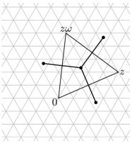
(b) step (i) $\triangle(0,z,\omega z)$

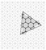
(c) step (ii) $\overline{\triangle}_{k,l}(p)$

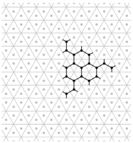
(d) $V(\triangle_{k,l}(p))$

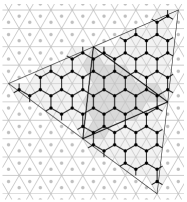
(e) glue $\overline{\triangle}_{k,l}(p)$ and $\overline{\triangle}_{k,l}(q_{i})$

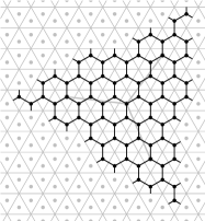
(f) $V(\triangle_{k,l}(p))\cup V(\triangle_{k,l}(q_{i}))$

Figure 1. In case of $(k,l)=(3,2)$, the Goldberg-Coxeter construction for a 3-valent graph around a vertex $p$ of the graph. By this procedure, we construct $V(\triangle_{k,l}(p))$ (see also Figure 2 and Section 2.1.1).

Proposition 2.2.

Let $X$ be a connected, finite and simple $3$- or $4$-valent graph which is embedded in an oriented surface $M$ in such a way that the closure of each face is simply connected. Then for $(k,l)\in\mathbb{Z}^{2}$, $(k,l)\neq(0,0)$, $\operatorname{GC}_{k,l}(X)$ is well-defined and is also embedded in $M$.

Proof.

The oriented tangent plane to $M$ at $p\in V(X)$ defines the orientation at $p$, and $\operatorname{GC}_{k,l}(X)$ is defined. The notion of faces is also well-defined. Since each face of $X$ is simply connected, we can take a dual graph $D_{X}$ of $X$ in $M$, all of whose faces are simply connected triangles (resp. rectangles) for the $3$-valent case (resp. $4$-valent case). The dividing step (ii) and the gluing step (iii) in Definition 2.1 are well done in $M$ via respective appropriate local charts. ∎

A Goldberg-Coxeter construction $\operatorname{GC}_{k,l}(X)$ for $3$-valent (resp. $4$-valent) graph $X$ inserts some hexagons (resp. squares), according to its parameter $k$ and $l$, between each pair of original faces of $X$. The most famous example is a fullerene $C_{60}$, called also a buckminsterfullerene or a buckyball, which is nothing but $\operatorname{GC}_{1,1}(\text{Dodecahedron})$. This construction owes its name to the pioneering work [15] due to M. Goldberg, where a so-called Goldberg polyhedron (a convex polyhedron whose $1$-skeleton is a $3$-valent graph, consisting of hexagons and pentagons with rotational icosahedral symmetry $3$-valent graph as its $1$-skeleton) is studied and is proved to be of the form $\operatorname{GC}_{k,l}(\text{Dodecahedron})$ for some $k$ and $l$. A Goldberg-Coxeter construction for $3$- or $4$-valent plane graphs occurs in many other context; see [5] and the references therein. Several examples of Goldberg-Coxeter constructions for nonplanar $3$-valent (infinite or finite quotient) graphs, such as for carbon nanotubes and Mackay-like crystals, are provided in [21].

The following proposition summarizes few fundamental properties of Goldberg-Coxeter constructions.

Proposition 2.3 (Deza-Dutour [5, 6]).

Let $X=(V(X),E(X))$ be a $3$-valent (resp. $4$-valent) graph equipped with an orientation at each vertex. Then the following hold.

1. If $X$ is embedded in an oriented surface in such a way that the closure of each face is simply connected, and the orientation at each vertex coincides with the one of the surface, then $\operatorname{GC}_{z}(\operatorname{GC}_{z^{\prime}}(X))=\operatorname{GC}_{zz^{\prime}}(X)$, for any $z,z^{\prime}\in\mathbb{Z}[\omega]$ (resp. $z,z^{\prime}\in\mathbb{Z}[i]$).

2. For any $(k,l)\in\mathbb{Z}^{2}$, $(k,l)\neq(0,0)$, we have the following graph isomorphisms:

   $$\operatorname{GC}_{k,l}(X)\simeq\operatorname{GC}_{-l,k+l}(X)\simeq\operatorname{GC}_{-k-l,k}(X)\simeq\operatorname{GC}_{-k,-l}(X)\simeq\operatorname{GC}_{l,-k-l}(X)\simeq\operatorname{GC}_{k+l,-k}(X),$$

   $$\operatorname{GC}_{k,l}(X)\simeq\operatorname{GC}_{l,k}(X).$$

   So $\{\operatorname{GC}_{k,l}(X)\mid k\geq l\geq 0,\ k\neq 0\}$ gives a system of representatives of graph isomorphism classes.

3. The number of vertices of $\operatorname{GC}_{z}(X)$ is given as $\lvert{V(\operatorname{GC}_{z}(X))}\rvert=\lvert z\rvert^{2}\lvert{V(X)}\rvert=(k^{2}+kl+l^{2})\lvert{V(X)}\rvert$, where $z=k+l\omega$ (resp. $\lvert{V(\operatorname{GC}_{z}(X))}\rvert=\lvert z\rvert^{2}\lvert{V(X)}\rvert=(k^{2}+l^{2})\lvert{V(X)}\rvert$, where $z=k+li$).

Deza-Dutour ([5, 6]) mentioned these properties only for plane graphs. However, these come from properties of triangular lattices and hence these also hold for graphs on oriented surfaces. In consideration of Proposition 2.3 (2), in the rest of this paper, we assume that $k$ is a positive integer and $l$ is a nonnegative integer satisfying $k\geq l\geq 0$ and $k\neq 0$.

2.1. Clusters for Goldberg-Coxeter constructions

A cluster is the central notion in this paper. Its definitions shall be given below in two different cases: where $X$ is $3$-valent and where $X$ is $4$-valent.

2.1.1. The case where $X$ is $3$-valent

For each $p\in V(X)$, let us construct a subgraph $\triangle_{k,l}(p)=(V(\triangle_{k,l}(p)),E(\triangle_{k,l}(p)))$ of $\overline{\triangle}_{k,l}(p)\subseteq\operatorname{GC}_{k,l}(X)$, called the $(k,l)$-cluster, so as to have $k^{2}+kl+l^{2}$ vertices and the $2\pi/3$-rotational symmetry of $\overline{\triangle}_{k,l}(p)$. For this, we just have to define $V(\triangle_{k,l}(p))$ by the set of vertices $x$ of $\overline{\triangle}_{k,l}(p)$ (considered as the graph on $\triangle\subseteq\mathbb{Z}[\omega]$) satisfying one of the following conditions:

1. $x\in\overline{\triangle}_{k,l}(p)$ corresponds to a triangle in $\mathbb{Z}[\omega]$ whose barycenter lies in the interior of $\triangle=\triangle(0,z,\omega z)$, where $z=k+l\omega$;

2. $x\in\overline{\triangle}_{k,l}(p)$ corresponds to an upward triangle in $\mathbb{Z}[\omega]$ whose barycenter lies on an edge of $\triangle$.

Here we mean an upward triangle $\triangle(a,b)$ by the triangle in $\mathbb{Z}[\omega]$ with vertices $a+b\omega$, $a+1+b\omega$ and $a+(b+1)\omega$ for $a,b\in\mathbb{Z}$ (see Figure 2). We also denote by $\rotatebox[origin={c}]{180.0}{$\triangle$}(a,b)$, called downward triangle, the triangle with vertices $a+b\omega$, $a+(b+1)\omega$ and $a-1+(b+1)\omega$.

In the case that $l=0$, $\triangle_{k,0}(p)$ is nothing but $\overline{\triangle}_{k,0}(p)$ itself, has $k^{2}$ vertices and has the dihedral symmetry $D_{3}$ (of order $6$) (see Figure 2).

In the case that $k=l>0$, it is easily seen that there are $3(k^{2}-k)$ vertices satisfying (i) and $3k$ vertices satisfying (ii). The obtained subgraph $\triangle_{k,k}(p)$ has $3k^{2}$ vertices and has the $2\pi/3$-rotational symmetry because upward triangles are mapped to upward triangles by the rotation (see Figure 2).

The following lemma makes clear the cases where there is a barycenter lying on an edge of $\triangle$ among the remaining cases.

Lemma 2.4.

Let $k>l>0$, $m:=\gcd(k,l)$, $k_{1}:=k/m$ and $l_{1}:=l/m$. An edge of the triangle $\triangle=\triangle(0,z,\omega z)$, where $z=k+l\omega$ in $\mathbb{Z}[\omega]$ passes through a barycenter of a small triangle in $\mathbb{Z}[\omega]$ if and only if

(2.1) $$k_{1}\not\equiv 0\pmod{3},\qquad k_{1}\equiv l_{1}\pmod{3}.$$

Moreover, in the case above, each edge of $\triangle$ passes through exactly $2m=2\gcd(k,l)$ barycenters. Among these $2m$ vertices, exactly $m$ vertices corresponding to upward triangles have just two adjacent triangles with barycenters lying in $\triangle$. The combined $3m$ vertices on the three edges of $\triangle$ are located in symmetric position with the rotation by $2\pi/3$ of $\triangle$.

Lemma 2.4 shows that the subgraph $\triangle_{k,l}(p)$ has $(k-l)^{2}+3kl=k^{2}+kl+l^{2}$ vertices and also has the $2\pi/3$-rotational symmetry in the remaining case that $k>l>0$.

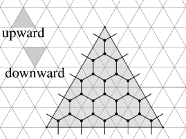
(a) $(k,l)=(5,0)$

(b) $(k,l)=(3,3)$

(c) $(k,l)=(4,1)$

Figure 2. $3$-valent $(k,l)$-clusters; $V(\triangle_{k,l}(p))$ consists of the barycenters of the gray triangles.

Here we can prove the following proposition, which guarantees that the bipartiteness is kept after a Goldberg-Coxeter construction.

Proposition 2.5.

Let $X$ be a $3$-valent bipartite graph equipped with an orientation at each vertex. Then for any $(k,l)\in\mathbb{Z}^{2}$, $(k,l)\neq(0,0)$, $\operatorname{GC}_{k,l}(X)$ is also bipartite. So the spectrum of $\operatorname{GC}_{k,l}(X)$ is symmetric with respect to $3$.

Proof.

Let a bipartition of $X$ be given and either black or white be assigned to each vertex $p\in V(X)$. Each vertex $x$ of each $\triangle_{k,l}(p)$ can be colored according to a rule that if $p$ is white, then

• paint $x$ black, provided the triangle in $\mathbb{Z}[\omega]$ corresponding to $x$ is upward;

• paint $x$ white, provided the triangle in $\mathbb{Z}[\omega]$ corresponding to $x$ is downward;

and if $p$ is black, then exchange black and white above. A white vertex is adjacent only to black vertices in $X$, and two adjacent clusters $\triangle_{k,l}(p)$ and $\triangle_{k,l}(q)$ are positioned, in $\mathbb{Z}[\omega]$, at $\pi$-rotation around the midpoint of an edge of $\triangle$, which switches upward and downward triangles. So, the rule above gives a bipartition of $\operatorname{GC}_{k,l}(X)$. ∎

2.1.2. The case where $X$ is $4$-valent

Similarly as in the $3$-valent case, we construct for each $p\in V(X)$ an appropriate subgraph $\square_{k,l}(p)=(V(\square_{k,l}(p)),E(\square_{k,l}(p)))$ of $\overline{\square}_{k,l}(p)$, still called the $(k,l)$-cluster, so as to have $k^{2}+l^{2}$ vertices. To this end, we need to clarify the cases where a barycenter of a small square in $\mathbb{Z}[i]$ lies on an edge of $\square=\square(0,z,(1+i)z,iz)$, where $z=k+li$.

For $a,b\in\mathbb{Z}$, we denote by $\square(a,b)$ the small square in $\mathbb{Z}[i]$ with vertices $a+bi,(a+1)+bi,(a+1)+(b+1)i,a+(b+1)i$, whose barycenter is given as $a+1/2+(b+1/2)i$.

Lemma 2.6.

Let $k\geq l\geq 0$, $k\neq 0$, $m:=\gcd(k,l)$, $k_{1}:=k/m$ and $l_{1}:=l/m$. An edge of the square $\square=\square(0,z,(1+i)z,iz)$, where $z=k+li$ in $\mathbb{Z}[i]$ passes through a barycenter of a small square in $\mathbb{Z}[i]$ if and only if

(2.2) $$k_{1}\not\equiv 0\pmod{2},\qquad k_{1}\equiv l_{1}\pmod{2}$$

Moreover, if this is the case, each edge of $\square$ passes through exactly $m$ barycenters.

Unlike the $3$-valent case, we cannot choose a cluster $\square_{k,l}(p)$ with $k^{2}+l^{2}$ vertices to have the $\pi/2$-rotational symmetry in the case where $k_{1}\not\equiv 0\pmod{2}$, $k_{1}\equiv l_{1}\pmod{2}$ and $m\not\equiv 0\pmod{2}$ because no vertex of $\overline{\square}_{k,l}(p)$ is positioned at the barycenter of $\square$ and $k^{2}+l^{2}=m^{2}((k_{1}-l_{1})^{2}+2k_{1}l_{1})$ is not divided by $4$. Even in such cases, $\square_{k,l}(p)$ only has to have the same number of outward edges among the four directions to every adjacent cluster.

Lemma 2.7 (cf. [14, Corollary IV.6]).

Let $X$ be a $4$-valent graph equipped with an orientation at each vertex. Then there exists an Euler circuit $\varepsilon$ of $X$ which turns either left or right at every vertex of $X$.

We note that the Euler circuit mentioned in Lemma 2.7 is an example of $A$-trails introduced in [14].

Proof.

As is well-known, any $4$-valent graph $X$ has an Euler circuit, which is by definition a closed path in $X$ which visits every edge exactly once. Let us take an Euler circuit $\varepsilon$ of $X$ and suppose that $\varepsilon$ goes straight ahead at a vertex $p\in V(X)$. The circuit $\varepsilon$ comes back to $p$ again from one of the other directions after it straight ahead at $p$ (because $X$ is $4$-valent). By following the interval in opposite directions, the obtained circuit goes straight ahead one time fewer than $\varepsilon$. This proves Lemma 2.7. ∎

The Euler circuit $\varepsilon$ obtained in Lemma 2.7 assigns a direction to each edge of $X$ such that the direction alternates between inward and outward at each vertex of $X$.

Now we can clearly define $V(\square_{k,l}(p))$ by the set of vertices $x$ of $\overline{\square}_{k,l}(p)$ satisfying one of the following conditions:

1. $x$ corresponds to a square in $\mathbb{Z}[i]$ whose barycenter lies in the interior of $\square$;

2. $x$ corresponds to a barycenter lying on the two edges of $\square$ with opposite sides which correspond to the outward edges of $X$ with respect to the Euler circuit $\varepsilon$ in Lemma 2.7.

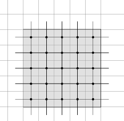
(a) $(k,l)=(5,0)$

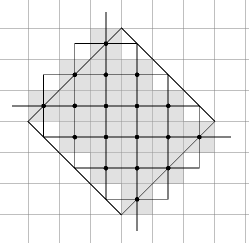
(b) $(k,l)=(3,3)$

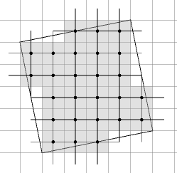
(c) $(k,l)=(5,1)$

Figure 3. $4$-valent $(k,l)$-clusters; $V(\square_{k,l}(p))$ consists of the barycenters of the gray squares.

2.2. Specific conditions on $3$-valent plane graphs

In this subsection a graph $X$ is assumed to be $3$-valent and embedded in a plane, and we study some structure of Goldberg-Coxeter constructions of $X$. Let us consider the following four conditions on $X$, which is, as shall be seen in Section 5.3, related to the multiplicities of certain eigenvalues of Goldberg-Coxeter constructions.

1. The number of edges surrounding each face is divisible by $3$.

2. For each vertex $p\in V(X)$, the numbers $1,2$ and $3$ are assigned in this order, with respect to the positive orientation, to the three edges of $X$ with $p$ as the common endpoint.

3. There exists a vertex numbering $V(\operatorname{GC}_{2,0}(X))\rightarrow\{1,2,3\}$ with the following properties:

   1. The number $0$ is assigned to the center of each $V(\triangle_{2,0}(p))$ ($p\in X$);

   2. the number assigned to $x\in V(\operatorname{GC}_{2,0}(X))$ is different from those of the adjacent vertices in $\operatorname{GC}_{2,0}(X)$ of $x$.

4. $V(X)$ can be colored by two colors, say black and white, with the following properties:

   1. A black vertex is adjacent to three white vertices;

   2. a white vertex is adjacent to exactly one black vertex, so the other two adjacent vertices are white;

   3. for any pair of black vertices $x,y\in V(X)$ which are three vertices away from each other, there is a path from $x$ to $y$ either turning left twice or turning right twice.

Remark 2.8.

We remark that

1. the condition (N) determines a special $3$-edge-coloring of $\operatorname{GC}_{2,0}(X)$, but a graph with $3$-edge-coloring does not necessarily satisfy (N),

2. a $3$-valent plane graph which satisfies the condition (F) is known to be a covering graph of the $K_{4}$ graph. (This fact is proved also from Proposition 2.9 below. )

The coherent edge numbering (CN) implies the condition (N); indeed, let $p\in V(X)$ and let $e_{1},e_{2}$ and $e_{3}$ be three edges of $X$ emanating from $p$. We assign $0$ to $p$ regarded as a vertex of $\operatorname{GC}_{2,0}(X)$, and, for $i=1,2$ and $3$, assign $i$ to the vertex of $\operatorname{GC}_{2,0}(X)$ positioned at the “opposite-side” to $e_{i}$. The resulting numbering of vertices of $\operatorname{GC}_{2,0}(X)$ satisfies (N-i) and (N-ii) (see Figure 4). Moreover, as is easily proved, (N) implies the condition (F). So the following proposition shows that (F), (CN) and (N) are mutually equivalent.

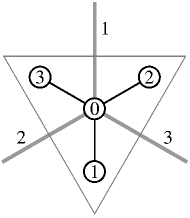
Figure 4. The gray (resp. black) segments represent edges of $X$ (resp. $\operatorname{GC}_{2,0}(X)$).

Proposition 2.9.

Let $X$ be a $3$-valent plane graph satisfying (F). Then $X$ has a coherent edge numbering $E(X)\rightarrow\{1,2,3\}$ satisfying (CN).

Proof.

For a sequence $e_{1},e_{2},\dots,e_{k}\in E(X)$ of adjacent edges in $X$ (namely $e_{i}\neq e_{i+1}$ and they have a common endpoint), we denote by $(e_{1},e_{2},\dots,e_{k})$ the path along the edges starting from $m(e_{1})$, the midpoint of $e_{1}$, and ending with $m(e_{k})$. To get a desired numbering $\nu\colon E(X)\rightarrow\{1,2,3\}$, we fix an edge $e_{0}\in E(X)$, and assign $3$ to $e_{0}$. For adjacent edges $e,e^{\prime}\in E(X)$ with the common endpoint $p$, let us define $\tau(e,e^{\prime})$ as

(2.3) $$\tau(e,e^{\prime}):=\left\{\begin{aligned} &+1,&&\text{if the path $(e,e^{\prime})$ turns right at $p$},\\ &-1,&&\text{if the path $(e,e^{\prime})$ turns left at $p$},\end{aligned}\right.$$

Note that $\tau(e,e^{\prime})=-\tau(e^{\prime},e)$. We then define $\nu\colon E(X)\rightarrow\{1,2,3\}$ for $e\in E(X)$ as

(2.4) $$\nu(e):=\sum_{i=1}^{n}\tau(e_{i-1},e_{i})\pmod{3}$$

by choosing a path $\gamma=(e_{0},e_{1},\dots,e_{n-1},e_{n}=e)$ from $e_{0}$ to $e$. What we have to prove is that $\nu(e)$ is independent of the choice of $\gamma$. To this end, let $\mathcal{P}(X,e_{0})$ be the set of sequences of adjacent edges in $X$ beginning with $e_{0}$ and let $\varphi\colon\mathcal{P}(X,e_{0})\rightarrow\{1,2,3\}$ be a map defined as

$$\varphi(\gamma):=\sum_{i=1}^{n}\tau(e_{i-1},e_{i})\pmod{3},\quad\text{for $\gamma=(e_{0},e_{1},\dots,e_{n})\in\mathcal{P}(X,e_{0})$}.$$

Note that for any $\gamma=(e_{0},e_{1},\dots,e_{n}),\gamma^{\prime}=(e_{0},e_{1}^{\prime},\dots,e_{m-1}^{\prime},e_{n})\in\mathcal{P}(X,e_{0})$, the joined (closed) path $\gamma^{\prime-1}\cdot\gamma=(e_{0},e_{1},\dots,e_{n},e_{m-1}^{\prime},\dots,e_{1}^{\prime},e_{0})$ satisfies

$$\varphi(\gamma^{\prime-1}\cdot\gamma)\equiv\varphi(\gamma)-\varphi(\gamma^{\prime})\pmod{3}.$$

Thus to prove that the map $\nu$ defined by (2.4) is well-defined, it suffices to see that $\varphi(\gamma)=3$ for any closed path $\gamma=(e_{0},e_{1},\dots,e_{n}=e_{0})$. Notice that $\varphi$ has the same image after removing a “back-tracking” part, that is, if $\gamma=(e_{0},\dots,e_{i-1},e_{i},e_{i+1},\dots,e_{0})$ contains a triplet of mutually adjacent edges $e_{i-1}$, $e_{i}$ and $e_{i+1}$, then

$$\varphi(\gamma)\equiv\varphi(e_{0},\dots,e_{i-2},e_{i+2},\dots,e_{0})\pmod{3},$$

and if $\gamma=(e_{0},\dots,e_{i-1},e_{i},e_{i+1},\dots,e_{0})$ satisfies $e_{i-1}=e_{i+1}$, then

$$\varphi(\gamma)\equiv\varphi(e_{0},\dots,e_{i-1},e_{i+2},\dots,e_{0})\pmod{3}.$$

Therefore the restriction $\varphi\colon\mathcal{CP}(X,e_{0})\rightarrow\{1,2,3\}$ of $\varphi$ to $\mathcal{CP}(X,e_{0})$, the set of closed paths with base edge $e_{0}$, descends to a homomorphism

$$\overline{\varphi}\colon\pi_{1}(X,m(e_{0}))\rightarrow\{1,2,3\},$$

where $\pi_{1}(X,m(e_{0}))$ is the fundamental group of $X$ with base point $m(e_{0})$. Since $\{1,2,3\}=\mathbb{Z}/3\mathbb{Z}$ is an abelian group, $\overline{\varphi}$ further descends to a homomorphism

$$\widetilde{\varphi}\colon H_{1}(X,\mathbb{Z})\rightarrow\{1,2,3\},$$

where $H_{1}(X,\mathbb{Z})$ is the $1$-dimensional homology group of $X$. Now any $\gamma\in H_{1}(X,\mathbb{Z})$ can be written as $\gamma=\sum_{f\colon\text{face of $X$}}a_{f}\partial f$, where $a_{f}\in\mathbb{Z}$ and $\partial f$ is the cycle consisting of edges around $f$. Our assumption implies that $\widetilde{\varphi}(\partial f)=3$ for any face $f$ of $X$. Hence we conclude that $\widetilde{\varphi}\equiv 3$, which implies that $\varphi\equiv 3$ on $\mathcal{CP}(X,e_{0})$. ∎

A relation between (F) and (C) is stated as follows.

Proposition 2.10.

Let $X$ be a $3$-valent plane graph satisfying (F). Then $X$ has a vertex coherent coloring satisfying (C-i), (C-ii) and (C-iii).

Proof.

Let $p_{0}\in V(X)$ be an arbitrary fixed vertex and color it black. Every vertex which is accessible by either turning left twice or turning right twice from a black vertex is, one after another, colored in black until no more vertices can be colored in black. The remaining vertices are colored in white. Now we have to check that (C-i) and (C-ii) are satisfied (while (C-iii) is necessarily satisfied). It is easily seen that a white vertex is adjacent to at least one black vertex; otherwise, all vertices of $X$ must be white. It is also easily checked that if a white vertex is adjacent to two or more black vertices, then two other black vertices are necessarily adjacent somewhere else. So, it suffices to show that any pair of black vertices cannot be adjacent.

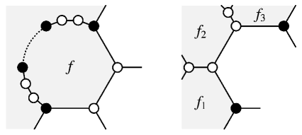
Figure 5. A Part of $\gamma$ where $\gamma$ turns left twice (left) and a part of $\gamma$ where $\gamma$ turns right twice (right). The gray regions are bounded ones surrounded by $\gamma$.

Suppose that there is a pair of adjacent black vertices, say $p,q\in V(X)$. From our way of the coloring, there is a path $\gamma$ from $p$ to $q$ which is a sequence of either twice turning left or twice turning right between black vertices. Then $\gamma\cup(q,p)$ is a closed path, which surrounds a finitely many faces, say $f_{1},f_{2},\dots,f_{n}$, after removing back-trackings. Now if $n=1$, then $\gamma$ consists of a circuit on the boundary $\partial f_{1}$ of a face $f_{1}$ and of some back-trackings with black base points on $\partial f_{1}$, which is a contradiction because the total of $\tau$ defined by (2.3) is $0\pmod{3}$ after the crossing just prior to a lap of $\gamma\cup(q,p)$. So assume that $n\geq 2$. There are just two possibilities of paths along the boundary of $\bigcup_{i=1}^{n}f_{i}$ connecting a pair of black vertices with distance $3$, as indicated in Figure 5. In either case, we can replace $\gamma\cup(q,p)$ by a closed path which does not surround a face $f_{i}$ (by ignoring back-trackings), and is still a sequence of either twice turning left or twice turning right between black vertices. Therefore the conclusion for the case where $n\geq 2$ can be deduced from the discussion given for the case $n=1$. ∎

Examples 2.11.

1. The tetrahedron and any of its Goldberg-Coxeter constructions satisfy all the conditions above.

2. $\operatorname{GC}_{2,0}(X)$ for any $3$-valent plane graph $X$ always satisfies (C-i), (C-ii) and (C-iii); indeed, we just have to color only the “center” of each $(2,0)$-cluster black, and the others white.

   

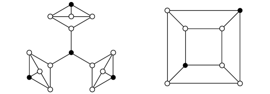
   Figure 6. Left coloring satisfies (C-i), (C-ii) and (C-iii). Right coloring on the cube satisfies (C-i) and (C-ii) but does not satisfy (C-iii).

3. $\operatorname{GC}_{1,1}(X)$ for any $3$-valent plane graph $X$ also always satisfies (C-i), (C-ii) and (C-iii); indeed, we just have to color in accordance with the rule shown in Figure 7.

   

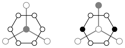
   Figure 7. Colorings for the $(1,1)$-cluster around a black (gray in this figure) vertex of $X$ (left) and a white one of $X$ (right). (The gray graphs represent for $X$, while black ones for $\operatorname{GC}_{1,1}(X)$. )

4. The cube satisfies (C-i) and (C-ii) but does not satisfy (C-iii) (see Figure 6), nor, of course, (F).

5. The dodecahedron satisfies none of the conditions above.

3. Two comparisons of the eigenvalues

In this section we give two kinds of comparisons of the eigenvalues, one is that between the eigenvalues of $X$ and those of $\operatorname{GC}_{k,l}(X)$, and the other is that between the eigenvalues of the $(k,0)$-cluster and those of $\operatorname{GC}_{k,0}(X)$. The former comparison provides the proof of Theorems 1.2, and the latter is used in the proof of Theorem 1.1. Throughout this section, let $k$ and $l$ be integers satisfying $k\geq l\geq 0$ and $k\neq 0$ in consideration of Proposition 2.3 (2).

3.1. The case where $X$ is $3$-valent

Proof of (1.1) and (1.2) in Theorem 1.2.

Let us denote by $V(p):=V(\triangle_{k,l}(p))$ for a fixed pair $(k,l)$. Let $p\in V(X)$, $q\in N_{X}(p)$ and set

(3.1) $$V_{0}(p):={} \left\{x\in V(p)\mathrel{}\middle|\mathrel{}N_{X^{\prime}}(x)\subseteq V(p)\right\},$$

$$V_{i}^{q}(p):={} \left\{x\in V(p)\mathrel{}\middle|\mathrel{}\lvert{N_{X^{\prime}}(x)\cap V(q)}\rvert=i\right\}\quad(i=1,2).$$

Note that, for any $x\in V(p)$ and $q\in N_{X}(p)$, there are at most two edges emanating from $x$ to $V(q)$. Since there is nothing to discuss when $(k,l)=(1,0)$, we only consider the other cases. Let $c=1/\sqrt{\lvert{V(p)}\rvert}=1/\sqrt{k^{2}+kl+l^{2}}$ and define a linear map $Q\colon\mathbb{C}^{V(X)}\rightarrow\mathbb{C}^{V(X^{\prime})}$ for $f\in\mathbb{C}^{V(X)}$ and for $x\in V(p)$ by

(3.2) $$(Qf)(x):=cf(p).$$

The transpose ${}^{\mathrm{t}}Q\colon\mathbb{C}^{V(X^{\prime})}\rightarrow\mathbb{C}^{V(X)}$ of $Q$ is then written as

$$({}^{\mathrm{t}}Qg)(p)=c\sum_{x\in V(p)}g(x)$$

for $g\in\mathbb{C}^{V(X^{\prime})}$ and $p\in V(X)$. It then follows that for any $f\in\mathbb{C}^{V(X)}$ and for any $p\in V(X)$,

$$({}^{\mathrm{t}}QQf)(p)=c\sum_{x\in V(p)}(Qf)(x)=c^{2}\sum_{x\in V(p)}f(p)=f(p),$$

that is ${}^{\mathrm{t}}QQ=\operatorname{id}_{\mathbb{C}^{V(X)}}$. Also, for arbitrary $f\in\mathbb{C}^{V(X)}$,

$$({}^{\mathrm{t}}Q\Delta_{X^{\prime}}Qf)(p)={} c\sum_{x\in V(p)}(\Delta_{X^{\prime}}Qf)(x)$$

$$={} c\sum_{x\in V(p)}\left\{3(Qf)(x)-\sum_{y\in N_{X^{\prime}}(x)}(Qf)(y)\right\}$$

$$={} 3c^{2}\lvert{V(p)}\rvert f(p)-c\sum_{x\in V_{0}(p)}\sum_{y\in N_{X^{\prime}}(x)}(Qf)(y)-c\sum_{x\in V(p)\setminus V_{0}(p)}\sum_{y\in N_{X^{\prime}}(x)}(Qf)(y).$$

The second term equals $-3c^{2}\lvert{V_{0}(p)}\rvert f(p)$ and the third term is computed as

$$c\sum_{x\in V(p)\setminus V_{0}(p)}\sum_{y\in N_{X^{\prime}}(x)}(Qf)(y)={} c\sum_{q\in N_{X}(p)}\sum_{x\in V_{1}^{q}(p)}\sum_{y\in N_{X^{\prime}}(x)}(Qf)(y)+c\sum_{q\in N_{X}(p)}\sum_{x\in V_{2}^{q}(p)}\sum_{y\in N_{X^{\prime}}(x)}(Qf)(y)$$

$$={} c^{2}\sum_{q\in N_{X}(p)}\lvert{V_{1}^{q}(p)}\rvert\left(2f(p)+f(q)\right)+c^{2}\sum_{q\in N_{X}(p)}\lvert{V_{2}^{q}(p)}\rvert\left(f(p)+2f(q)\right)$$

$$={} 3c^{2}(2\lvert{V_{1}^{q}(p)}\rvert+\lvert{V_{2}^{q}(p)}\rvert)f(p)+c^{2}(\lvert{V_{1}^{q}(p)}\rvert+2\lvert{V_{2}^{q}(p)}\rvert)\sum_{q\in N_{X}(p)}f(q),$$

where the last equality follows from the symmetry of $\triangle_{k,l}(p)$. Therefore we obtain

$$({}^{\mathrm{t}}Q\Delta_{X^{\prime}}Qf)(p)={} c^{2}(\lvert{V_{1}^{q}(p)}\rvert+2\lvert{V_{2}^{q}(p)}\rvert)(\Delta_{X}f)(p)$$

$$={} \frac{\mu(k,l)}{k^{2}+kl+l^{2}}(\Delta_{X}f)(p),$$

where $\mu(k,l)$ is the number of edges in $X^{\prime}$ connecting two clusters and depends only on $k$ and $l$. It is easily proved that $\mu(k,0)=k$ and $\mu(k,k)=3k$. To estimate $\mu(k,l)$ when $k>l>0$, let us estimate the number of edges crossing the edge $E=0z$. Notice first that there is at most one crossing edge emanating from an upward triangle $\triangle(a,b)$, and that there are at most two crossing edge emanating from a downward triangle $\rotatebox[origin={c}]{180.0}{$\triangle$}(a,b)$. For $c\in\mathbb{Z}$, “the zigzag path” which is obtained by joining the barycenters of $\rotatebox[origin={c}]{180.0}{$\triangle$}(a,b)$, $\triangle(a,b)$ and $\rotatebox[origin={c}]{180.0}{$\triangle$}(a+1,b-1)$ for all $a,b\in\mathbb{Z}$ with $a+b=c$ crosses the edge $E=0z$ exactly once provided $0\leq c\leq k+l-1$ and does not cross $E$ otherwise. Also, the line passing through $a\in\mathbb{Z}$ with slant $1+\omega$ crosses $E$ exactly once provided $0\leq a\leq k-l$ and does not cross $E$ otherwise. Therefore the number of edges crossing $E$ is at most $k+l+(k-l-2)=2k-2$ (see Figure 8 for an example).

(1.1) of Theorem 1.2 now immediately follows from the following.

Theorem 3.1 (Interlacing property, see for example [2]).

Let $Q$ be a real $n\times m$ matrix satisfying ${}^{\mathrm{t}}QQ=I_{m}$ and $A$ be a real symmetric $n\times n$ matrix. If the eigenvalues of $A$ and ${}^{\mathrm{t}}QAQ$ are

$$\nu_{1}(A)\leq\nu_{2}(A)\leq\dots\leq\nu_{n}(A),\quad\nu_{1}({}^{\mathrm{t}}QAQ)\leq\nu_{2}({}^{\mathrm{t}}QAQ)\leq\dots\leq\nu_{m}({}^{\mathrm{t}}QAQ),$$

respectively, then

$$\nu_{j}(A)\leq\nu_{j}({}^{\mathrm{t}}QAQ)\leq\nu_{n-m+j}(A)\quad(j=1,2,\dots,m).$$

Figure 8. $(k,l)=(9,3)$. $15$ edges cross the edge $E=0z$, ($z=9+3\omega$).

(1.2) is an immediate consequence from (1.1) and Proposition 2.5. ∎

The eigenvalues of $\operatorname{GC}_{k,0}(X)$ are estimated, independently of the graph structure of $X$, also by those of the $(k,0)$-cluster as follows.

Theorem 3.2.

Let $X$ be a $3$-valent graph satisfying the same assumptions as in Theorem 1.2, and $\nu_{1}(k)\leq\nu_{2}(k)\leq\cdots\leq\nu_{k^{2}}(k)$ (resp. $0=\lambda_{1}(k)\leq\lambda_{2}(k)\leq\cdots\leq\lambda_{k^{2}}(k)$) be the eigenvalues of the adjacency matrix (resp. of the Laplacian) of the $3$-valent $(k,0)$-cluster. Then for $j=1,2,\dots,k^{2}$,

(3.3) $$\lambda_{j}(\operatorname{GC}_{k,0}(X))\leq 3-\nu_{k^{2}-j+1}(k),$$

(3.4) $$\lambda_{\lvert{V(\operatorname{GC}_{k,0}(X))}\rvert-j+1}(\operatorname{GC}_{k,0}(X))\geq 3-\nu_{j}(k).$$

Moreover, we have

(3.5) $$\lambda_{i}(\operatorname{GC}_{k,0}(X))\leq\lambda_{t}(k)+\delta_{k^{2}-t+i}(k),\quad\text{for $1\leq i\leq t\leq k^{2}$},$$

(3.6) $$\lambda_{\lvert{V(\operatorname{GC}_{k,0}(X))}\rvert-j+1}(\operatorname{GC}_{k,0}(X))\geq\lambda_{k^{2}-s+1}(k)+\delta_{1+s-j}(k),\quad\text{for $1\leq j\leq s\leq k^{2}$},$$

where $\delta_{j}(k)$ is given as

$$\delta_{j}(k)=\left\{\begin{aligned} &0,&&\text{for $j=1,2,\dots,k^{2}-3k+3$},\\ &1,&&\text{for $j=k^{2}-3k+4,\dots,k^{2}-3$},\\ &2,&&\text{for $j=k^{2}-2,k^{2}-1,k^{2}$}\end{aligned}\right.$$

Proof.

Let $p\in V(X)$ be fixed and let $\triangle(k)=\triangle(p)$ be the $(k,0)$-cluster, which is considered as a subgraph of $X_{k}=\operatorname{GC}_{k,0}(X)$. Let us define a linear map $Q\colon\mathbb{C}^{V(X_{k})}\rightarrow\mathbb{C}^{V(\triangle(k))}$ by

$$(Qf)(x):=\left\{\begin{aligned} &f(x),&&\text{if $x\in V(\triangle(k))$},\\ &0,&&\text{if $x\not\in V(\triangle(k))$}\end{aligned}\right.$$

for $f\in\mathbb{C}^{V(X_{k})}$ and $x\in V(X_{k})$. Then a simple computation shows ${}^{\mathrm{t}}QQ=\operatorname{id}_{\mathbb{C}^{V(X_{k})}}$ and ${}^{\mathrm{t}}QA_{X_{k}}Q=A_{\triangle(k)}$, where $A$’s denote the adjacency matrices. By noting that $X_{k}=\operatorname{GC}_{k,0}(X)$ is a $3$-regular graph, the interlacing property (Theorem 3.1) proves (3.3) and (3.4). Since

$${}^{\mathrm{t}}Q\Delta_{X_{k}}Q=\Delta_{\triangle(k)}+(3\operatorname{id}_{\mathbb{C}^{V(\triangle(k))}}-D_{k}),$$

where $D_{k}\colon\mathbb{C}^{V(\triangle(k))}\rightarrow\mathbb{C}^{V(\triangle(k))}$ is defined as $(Df)(x):=\deg(x)$ for $f\in\mathbb{C}^{V(\triangle(k))}$ and $x\in V(\triangle(k))$, Combining the Courant-Weyl inequality (cf. [2, Theorem 1.3.15]) and the interlacing property proves (3.5) and (3.6). ∎

3.2. The case where $X$ is $4$-valent

The proof of (1.1) for the $4$-valent case is almost same as that for $3$-valent case, and let us omit it. The comparison between the eigenvalues of a $(k,0)$-cluster and those of $\operatorname{GC}_{k,0}(X)$ for the $4$-valent case is stated as follows.

Theorem 3.3.

Let $X$ be a $4$-valent graph satisfying the same assumptions as in Theorem 1.2, and $\nu_{1}(k)\leq\nu_{2}(k)\leq\cdots\leq\nu_{k^{2}}(k)$ (resp. $0=\lambda_{1}(k)\leq\lambda_{2}(k)\leq\cdots\leq\lambda_{k^{2}}(k)$) be the eigenvalues of the adjacency matrix (resp. of the Laplacian) of the $4$-valent $(k,0)$-cluster. Then for $j=1,2,\dots,k^{2}$,

$$\lambda_{j}(\operatorname{GC}_{k,0}(X))\leq 4-\nu_{k^{2}-j+1}(k),$$

$$\lambda_{\lvert{V(\operatorname{GC}_{k,0}(X))}\rvert-j+1}(\operatorname{GC}_{k,0}(X))\geq 4-\nu_{j}(k),$$

Moreover, we have

$$\lambda_{i}(\operatorname{GC}_{k,0}(X))\leq\lambda_{t}(k)+\delta_{k^{2}-t+i}(k),\quad\text{for $1\leq i\leq t\leq k^{2}$},$$

$$\lambda_{\lvert{V(\operatorname{GC}_{k,0}(X))}\rvert-j+1}(\operatorname{GC}_{k,0}(X))\geq\lambda_{k^{2}-s+1}(k)+\delta_{1+s-j}(k),\quad\text{for $1\leq j\leq s\leq k^{2}$},$$

where $\delta_{j}(k)$ is given as

$$\delta_{j}(k)=\left\{\begin{aligned} &0,&&\text{for $j=1,2,\dots,k^{2}-4k+4$},\\ &1,&&\text{for $j=k^{2}-4k+5,\dots,k^{2}-4$},\\ &2,&&\text{for $j=k^{2}-3,k^{2}-2,k^{2}-1,k^{2}$}.\\ \end{aligned}\right.$$

Since the proof of this theorem is again almost same as that for the $3$-valent case, let us omit it.

4. Eigenvalues of the $(k,0)$-cluster

In this section we shall find all the eigenvalues of a $(k,0)$-cluster to prove Theorem 1.1. Since the $(k,0)$-clusters are, as abstract graphs, isomorphic to each other, fixing a vertex $p\in V(X)$, we may denote it by $\triangle(k):=\triangle_{k,0}(p)=\overline{\triangle}_{k,0}(p)$ or $\square(k):=\square_{k,0}(p)=\overline{\square}_{k,0}(p)$.

4.1. The case where $X$ is $3$-valent

Definition 4.1.

$\lambda\geq 0$ is called a $D_{3}$-invariant eigenvalue (resp. $D_{3}$-alternating eigenvalue) for a $(k,0)$-cluster $\triangle(k)$ if there exists a non-zero function $u\colon V(\triangle(k))\rightarrow\mathbb{C}$, called a $D_{3}$-invariant eigenfunction (resp. $D_{3}$-alternating eigenfunction), with the following properties.

1. $u$ solves $(\Delta_{\triangle(k)}u)(x)=\lambda u(x)$ for $x\in V(\triangle(k))$

2. $u(\sigma x)=u(x)$ (resp. $u(\sigma x)=\operatorname{sgn}(\sigma)u(x)$) for $x\in V(\triangle(k))$, where $\sigma\colon\triangle(k)\rightarrow\triangle(k)$ is an element of the dihedral group $D_{3}$ and $\operatorname{sgn}(\sigma)$ denotes its signature.

Remarks 4.2.

(1) The following remark shall be repeatedly used in the sequel: by assigning the same function $u$ to the other clusters, we have a global function $u\colon\operatorname{GC}_{k,0}(X)\rightarrow\mathbb{C}$, which is an eigenfunction of $\Delta_{\operatorname{GC}_{k,0}(X)}$ with eigenvalue $\lambda$; indeed, (i) $\Delta_{\triangle(k)}u=\lambda u$ is equivalent to a Neumann problem:

(4.1) $$\left\{\begin{aligned} &(\Delta_{\operatorname{GC}_{k,0}(X)}u)(x)=\lambda u(x),&&\text{for $x\in V(p)$},\\ &u(y)-u(x)=0,&&\text{for $x\in V(p)\setminus V_{0}(p)$ and $y\in N_{\operatorname{GC}_{k,0}(X)}(x)\setminus V(p)$}\end{aligned}\right.$$

for some/any $p\in V(X)$.

(2) There is no eigenfunction on a $(k,0)$-cluster which is both $D_{3}$-invariant and $D_{3}$-alternating.

Our first task is to find all the $D_{3}$-invariant eigenspaces, which proves Theorem 1.3 as well as (1.3) in Theorem 1.2. To this end, let us first construct all the eigenfunctions on a hexagonal lattice with toroidal boundary condition. If we set $\textsc{m}:=(1+\omega)/3$, where $\omega=e^{\pi i/3}$, then the discrete set

(4.2) $$\left\{a+b\omega\mathrel{}\middle|\mathrel{}a,b\in\mathbb{Z}\right\}\cup\left\{\textsc{m}+a+b\omega\mathrel{}\middle|\mathrel{}a,b\in\mathbb{Z}\right\}$$

is naturally regarded as a hexagonal lattice. For a fixed $k\in\mathbb{N}$, let us consider the equations

(4.3) $$3v(a+b\omega)-v(\textsc{m}+a+b\omega)-v(\textsc{m}+a-1+b\omega)-v(\textsc{m}+a+(b-1)\omega)=\lambda v(a+b\omega),$$

$$3v(\textsc{m}+a+b\omega)-v(a+b\omega)-v(a+1+b\omega)-v(a+(b+1)\omega)=\lambda v(\textsc{m}+a+b\omega)$$

for a function $v$ on the parallelogram

$$P(k):=\left\{a+b\omega\mathrel{}\middle|\mathrel{}0\leq a,b\leq k-1\right\}\cup\left\{\textsc{m}+a+b\omega\mathrel{}\middle|\mathrel{}0\leq a,b\leq k-1\right\},$$

where $a$ and $b$ in (4.3) are considered modulo $k$, such as

$$3v(0)-v(\textsc{m})-v(\textsc{m}+k-1)-v(\textsc{m}+(k-1)\omega)=\lambda v(0)$$

for the former equation of (4.3) with $a=b=0$. So if $v$ solves (4.3), then it gives an eigenfunction with eigenvalue $\lambda$ on the finite $3$-valent graph $T(k)$ with $2k^{2}$ vertices obtained by adding edges between $a$ and $\textsc{m}+a+(k-1)\omega$, and between $b\omega$ and $\textsc{m}+k-1+b\omega$ for each $a,b=0,1,\dots,k-1$.

A simple computation shows that an eigenvalue is of the form

(4.4) $$\lambda_{s,t}^{\pm}=\lambda_{s,t}^{\pm}(k)=3\pm\sqrt{3+2\cos\frac{2\pi s}{k}+2\cos\frac{2\pi t}{k}+2\cos\frac{2\pi(s-t)}{k}},$$

whose corresponding eigenfunction is given as

$$\left\{\begin{aligned} v_{s,t}^{\pm}(a+b\omega)={}&e^{2\pi i(sa+tb)/k},\\ v_{s,t}^{\pm}(\textsc{m}+a+b\omega)={}&\frac{1}{3-\lambda_{s,t}^{\pm}}v_{s,t}^{\pm}(a+b\omega)\left(1+e^{2\pi is/k}+e^{2\pi it/k}\right)\end{aligned}\right.$$

($a+b\omega,\textsc{m}+a+b\omega\in P(k)$) for $s,t=0,1,\dots,k-1$, unless $\lambda_{s,t}^{\pm}=3$. If $\lambda_{s,t}^{\pm}=3$, which is possible only if $k\equiv 0\pmod{3}$ and either $(s,t)=(k/3,2k/3)$ or $(2k/3,k/3)$ among the range $0\leq s,t\leq k-1$, then

$$\left\{\begin{aligned} v_{k/3,2k/3}(a+b\omega)={}&\alpha e^{2\pi i(a+2b)/3},\\ v_{k/3,2k/3}(\textsc{m}+a+b\omega)={}&\alpha^{\prime}e^{2\pi i(a+2b)/3},\end{aligned}\right.\quad\left\{\begin{aligned} v_{2k/3,k/3}(a+b\omega)={}&\beta e^{2\pi i(2a+b)/3},\\ v_{2k/3,k/3}(\textsc{m}+a+b\omega)={}&\beta^{\prime}e^{2\pi i(2a+b)/3},\end{aligned}\right.$$

where $\alpha,\alpha^{\prime},\beta,\beta^{\prime}\in\mathbb{C}$ are arbitrary, both define eigenfunctions for the eigenvalue $3$.

We now consider the following three maps defined on the hexagonal lattice:

• the rotation around $(k-1)(1+\omega)/3$ by $2\pi/3$: $\left\{\begin{aligned} &a+b\omega\mapsto k-a-b-1+a\omega,\\ &\textsc{m}+a+b\omega\mapsto\textsc{m}+k-a-b-2+a\omega,\end{aligned}\right.$

• the reflection along the long diagonal line of $P(k)$: $\left\{\begin{aligned} &a+b\omega\mapsto b+a\omega,\\ &\textsc{m}+a+b\omega\mapsto\textsc{m}+b+a\omega,\end{aligned}\right.$

• and the reflection along the short one: $\left\{\begin{aligned} &a+b\omega\mapsto\textsc{m}+k-b-1+(k-a-1)\omega,\\ &\textsc{m}+a+b\omega\mapsto k-b-1+(k-a-1)\omega.\end{aligned}\right.$

These maps define, by considering $a$ and $b$ modulo $k$, automorphisms on $T(k)$, and generate the dihedral group $D_{6}$ of order $12$. As is easily confirmed, taking the average $\sum_{\sigma\in D_{6}}\sigma f$ (resp. $\sum_{\sigma\in D_{6}}\operatorname{sgn}(\sigma)\sigma f$) for $f\in\mathbb{C}^{P(k)}$ defines a projection onto the $D_{3}$-invariant eigenspaces (resp. $D_{3}$-alternating eigenspaces) for the $(k,0)$-cluster, where $\operatorname{sgn}(\sigma)$ is the number modulo $2$ of the reflections along the long diagonal line of $P(k)$ in an expression of $\sigma$. Now we set, for $s,t=0,1,\dots,k-1$,

(4.5) $$u_{s,t}^{\pm}:=\sum_{\sigma\in D_{6}}\sigma v_{s,t}^{\pm}\quad\text{and}\quad w_{s,t}^{\pm}:=\sum_{\sigma\in D_{6}}\operatorname{sgn}(\sigma)\sigma v_{s,t}^{\pm},$$

which respectively give a $D_{3}$-invariant eigenfunction and a $D_{3}$-alternating eigenfunction on $\triangle(k)$ unless they identically vanish on $\triangle(k)$. Note that these functions respectively generate the space of $D_{3}$-invariant eigenfunctions and the one of $D_{3}$-alternating eigenfunctions because they define functions also on $T(k)$. The following Lemma 4.3 explicitly tells us when $u_{s,t}^{\pm}$ and $w_{s,t}^{\pm}$ vanish.

Lemma 4.3.

Let $0\leq s,t\leq k-1$. $u_{s,t}^{\pm}\equiv 0$ if and only if $u_{s,t}^{\pm}$ is one of the following:

• $u_{s,k-s}^{+}$ or $u_{k-s,s}^{+}$ for $1\leq s<k/3$;

• $u_{s,k-s}^{-}$ for $k/3<s<2k/3$;

• $u_{s,2s}^{+}$ or $u_{2s,s}^{+}$ for $0\leq s<k/3$;

• $u_{s,2s}^{-}$ or $u_{2s,s}^{-}$ for $k/3<s<k/2$;

• $u_{s,2s-k}^{-}$ or $u_{2s-k,s}^{-}$ for $k/2\leq s<2k/3$;

• $u_{s,2s-k}^{+}$ or $u_{2s-k,s}^{+}$ for $2k/3<s\leq k-1$.

On the other hand, $w_{s,t}^{\pm}\equiv 0$ if and only if $w_{s,t}^{\pm}$ is one of the following:

• $w_{s,0}^{\pm}$ or $w_{0,t}^{\pm}$ for $0\leq s,t\leq k-1$;

• $w_{s,s}^{\pm}$ for $0\leq s\leq k-1$;

• $w_{s,k-s}^{+}$ or $w_{k-s,s}^{+}$ for $1\leq s<k/3$

• $w_{s,k-s}^{-}$ for $k/3<s<2k/3$;

• $w_{s,2s}^{+}$ or $w_{2s,s}^{+}$ for $0\leq s<k/3$;

• $w_{s,2s}^{-}$ or $w_{2s,s}^{-}$ for $k/3<s<k/2$;

• $w_{s,2s-k}^{-}$ or $w_{2s-k,s}^{-}$ for $k/2\leq s<2k/3$;

• $w_{s,2s-k}^{+}$ or $w_{2s-k,s}^{+}$ for $2k/3<s\leq k-1$.

In particular the associated eigenvalues $\lambda_{s,t}^{\pm}$ other than the above lists give $D_{3}$-invariant or $D_{3}$-alternating eigenvalues, respectively.

Proof.

The proof uses explicit expression of $u_{s,t}^{\pm}$ and $w_{s,t}^{\pm}$ via the coordinate (4.2).

A direct computation shows that

$$u_{s,t}^{\pm}(0)\left(1+e^{4\pi is/k}+e^{4\pi it/k}\right)\left(1+e^{-2\pi is/k}+e^{-2\pi it/k}\right)$$

$$\pm u_{s,t}^{\pm}(\textsc{m})\left(1+e^{2\pi is/k}+e^{2\pi it/k}\right)\left|\left(1+e^{2\pi is/k}+e^{2\pi it/k}\right)\right|$$

$$={} -32i\sin\frac{\pi(s+t)}{k}\sin\frac{\pi(2s-t)}{k}\sin\frac{\pi(s-2t)}{k},$$

from which the above list for $u_{s,t}^{\pm}$ is obtained.

A direct computation shows that

$$w_{s,t}^{\pm}(1)\left(1+e^{2\pi is/k}+e^{2\pi it/k}+e^{2\pi i(s+t)/k}+e^{2\pi i(s-t)/k}+e^{2\pi i(t-s)/k}\right)$$

$$\pm w_{s,t}^{\pm}(\textsc{m}+1)\left(1+e^{2\pi is/k}+e^{2\pi it/k}\right)$$

$$={} 64\sin\frac{\pi s}{k}\sin\frac{\pi t}{k}\sin\frac{\pi(s-t)}{k}\sin\frac{\pi(s+t)}{k}\sin\frac{\pi(2s-t)}{k}\sin\frac{\pi(s-2t)}{k},$$

from which the above list for $w_{s,t}^{\pm}$ is obtained. ∎

Proof of (1.3) in Theorem 1.2.

Let us prove that if $\lambda\geq 0$ is a $D_{3}$-invariant eigenvalue for the $(k,0)$-cluster, then

(4.6) $$\lambda\leq\lambda_{\lvert{V(\operatorname{GC}_{k,0}(X))}\rvert-i+1}(\operatorname{GC}_{k,0}(X))$$

holds for $i=1,2,\dots,\lvert{V(X)}\rvert$.

Let $u\colon\operatorname{GC}_{k,0}(X)\rightarrow\mathbb{C}$ be an eigenfunction for the eigenvalue $\lambda$ which is obtained, as was explained in (1) of Remarks 4.2, from a $D_{3}$-invariant eigenfunction on the $(k,0)$-cluster. We may assume that $\sum_{x\in V(p)}u(x)^{2}=1$, so that ${}^{\mathrm{t}}QQ=\operatorname{id}_{\mathbb{C}^{V(X)}}$. Replacing $c$ in (3.2) by $u$, after a straightforward computation using (i) and (ii) in Definition 4.1 for $u$, we can obtain the following equality:

(4.7) $$({}^{\mathrm{t}}Q\Delta_{\operatorname{GC}_{k,0}(X)}Qf)(p)=\left\{\sum_{x\in V_{1}^{q}(p)}u(x)^{2}+2\sum_{x\in V_{2}^{q}(p)}u(x)^{2}\right\}(\Delta_{X}f)(p)+\lambda f(p)$$

for any $f\in\mathbb{C}^{V(X)}$ and any $p\in V(X)$, where $q\in N_{X}(p)$ is an adjacent vertex to $p$. (4.6) is proved again from the interlacing property (Theorem 3.1).

(1.3) is an immediate consequence of Lemma 4.3, which claims that

$$\lambda=\lambda_{1,0}^{+}=\lambda_{0,1}^{+}=3+\sqrt{5+4\cos\frac{2\pi}{k}}$$

is the largest $D_{3}$-invariant eigenvalue for the $(k,0)$-cluster. ∎

Proof of Theorem 1.3.

It follows from the consequence of Lemma 4.3 that

• $\lambda_{j,k-j}^{-}=3-\sqrt{3+4\cos\frac{2\pi j}{k}+2\cos\frac{4\pi j}{k}}$ for $0\leq j\leq\lceil k/3\rceil-1$;

• $\lambda_{\lfloor k/3\rfloor+j,k-\lfloor k/3\rfloor-j}^{+}=3+\sqrt{3+4\cos\frac{2\pi(\lfloor k/3\rfloor+j)}{k}+2\cos\frac{4\pi(\lfloor k/3\rfloor+j)}{k}}$ for $1\leq j\leq\lceil 2k/3\rceil-\lfloor k/3\rfloor-1$;

• $\lambda_{s,0}^{+}=3+\sqrt{5+4\cos\frac{2\pi s}{k}}$ for $1\leq s\leq k-1$

are all $D_{3}$-invariant eigenvalues for the $(k,0)$-cluster. In the expression of $\lambda_{s,0}^{+}$, set $x=s/k\in[0,1)$, then the function $3+\sqrt{5+4\cos(2\pi x)}$ takes value $[4,6]$. Taking large $k$, we may approximate any number $x\in[0,1)$ by $s/k$ ($0\leq s\leq k-1$), and an arbitrary real number in $[4,6]$ is approximated by $\lambda_{s,0}^{+}$. Similary an arbitrary real number in $[0,3]$ and $[3,4]$ is approximated by $\lambda_{j,k-j}^{-}$ and $\lambda_{\lfloor k/3\rfloor+j,k-\lfloor k/3\rfloor-j}^{+}$, respectively. Hence an arbitrary real number in $[0,6]$ is approximated by these values as $k$ tends to infinity. ∎

In order to prove Theorem 1.1 using Theorem 3.2, it suffices to find all the eigenvalues of a $(k,0)$-cluster. To achieve this, we notice that the set of all the eigenvalues of a $(k,0)$-cluster contains the set of all the $D_{3}$-invariant and all the $D_{3}$-alternating eigenvalues of the $(3k,0)$-cluster; indeed, we have a well-defined injection

$$\iota\colon\mathbb{C}^{\triangle(k)}\rightarrow\mathcal{U}_{3k}\oplus\mathcal{W}_{3k}$$

which is defined by the foldings like shown in Figure 9, where $\mathcal{U}_{3k}$ (resp. $\mathcal{W}_{3k}$) denotes the space of $D_{3}$-invariant (resp. $D_{3}$-alternating) eigenfunctions on the $(3k,0)$-cluster.

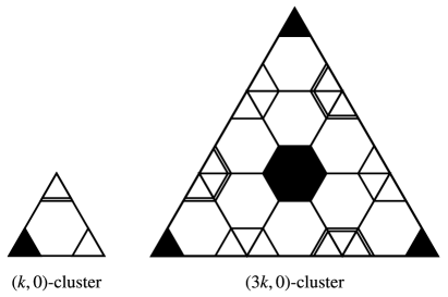
Figure 9. $\triangle(3k)$ is tiled by the foldings of $\triangle(k)$; if the function on $\triangle(k)$ is symmetric (resp. antisymmetric) w.r.t. the line $a=b$, then the obtained function lies in $\mathcal{U}_{3k}$ (resp. $\mathcal{W}_{3k}$).

Lemma 4.4.

$u_{s,t}^{\pm}\in\mathcal{U}_{3k}$ (resp. $w_{s,t}^{\pm}\in\mathcal{W}_{3k}$) lies in the image of $\iota$ if and only if $s+t$ is divisible by $3$. Moreover, if both $s$ and $t$ are divisible by $3$, then $u_{s,t}^{\pm}|_{\triangle(k)}$ (resp. $w_{s,t}^{\pm}|_{\triangle(k)}$) is also a $D_{3}$-invariant (resp. $D_{3}$-alternating) eigenfunction.

Outline of the Proof.

The proof again uses explicit expression of $u_{s,t}^{\pm}$ and $w_{s,t}^{\pm}$. Note first that $f=u_{s,t}^{\pm}$ or $w_{s,t}^{\pm}$ lies in the image of $\iota$ iff.

(4.8) $$f_{s,t}^{\pm}(a+b\omega)={} f_{s,t}^{\pm}(\textsc{m}+k-b-1+(k-a-1)\omega),$$

$$f_{s,t}^{\pm}(a+b\omega)={} f_{s,t}^{\pm}(\textsc{m}+2k-b-1+(2k-a-1)\omega)$$

for any $a,b$.

A direct computation similar to that in the proof of Lemma 4.3 shows that (4.8) for $f_{s,t}^{\pm}=u_{s,t}^{\pm}$ with $a=b=0$ implies

$$\left(1-e^{-2\pi i(s+t)/3}\right)\sin\frac{\pi(s+t)}{3k}\sin\frac{\pi(2s-t)}{3k}\sin\frac{\pi(s-2t)}{3k}=0,$$

which is valid only if $s+t$ is divisible by $3$.

A direct computation shows that (4.8) for $f_{s,t}^{\pm}=w_{s,t}^{\pm}$ with $(a,b)=(1,0)$ implies

$$\left(1-e^{-2\pi i(s+t)/3}\right)\sin^{2}\frac{\pi s}{3k}\sin^{2}\frac{\pi t}{3k}\sin^{2}\frac{\pi(s-t)}{3k}\sin\frac{\pi(s+t)}{3k}\sin\frac{\pi(2s-t)}{3k}\sin\frac{\pi(s-2t)}{3k}=0,$$

which is valid only if either $s=0$, $t=0$, $s=t$ or $s+t\equiv 0\pmod{3}$. The cases for $s=0$, $t=0$ and $s=t$ are excluded because then $w_{s,t}^{\pm}\equiv 0$. ∎

Proof of Theorem 1.1.

As is easily confirmed, $f_{s,t}^{\pm}=u_{s,t}^{\pm}$ or $w_{s,t}^{\pm}$ satisfies

$$f_{s,t}^{\pm}={} f_{t,s}^{\pm}=f_{t-s,t}^{\pm}=f_{t,t-s}^{\pm}=f_{3k-s,3k-t}^{\pm}=f_{3k-t,3k-s}^{\pm}$$

$$={} f_{3k-t+s,3k-t}^{\pm}=f_{3k-t,3k-t+s}^{\pm}=f_{3k-s,t-s}^{\pm}=f_{t-s,3k-s}^{\pm}=f_{s,3k-t+s}^{\pm}=f_{3k-t+s,s}^{\pm}$$

and therefore, by Lemmas 4.3 and 4.4, the image of $\iota$ is contained in the vector space, say $\mathcal{V}$, spanned by $u_{s,t}^{\pm}$’s for

(4.9) $$\left\{({\pm},s,t)\mathrel{}\middle|\mathrel{}\text{$s+t$ is divisible by $3$},\ 0<s<2k,\ \max\{0,2s-3k\}<t<s/2\right\}$$

$$\cup \left\{({-},2s,s)\mathrel{}\middle|\mathrel{}0\leq s<2k\right\}$$

$$\cup \left\{({+},s,2s-3k)\mathrel{}\middle|\mathrel{}3k/2\leq s<2k\right\}$$

$$\cup \left\{(\pm,s,0)\mathrel{}\middle|\mathrel{}\text{$s$ is divisible by $3$},\ 0<s<3k/2\right\}$$

and $w_{s,t}^{\pm}$’s for

(4.10) $$\left\{({\pm},s,t)\mathrel{}\middle|\mathrel{}\text{$s+t$ is divisible by $3$},\ 0<s<2k,\ \max\{0,2s-3k\}<t<s/2\right\}$$

$$\cup \left\{({-},2s,s)\mathrel{}\middle|\mathrel{}0\leq s<2k\right\}$$

$$\cup \left\{({+},s,2s-3k)\mathrel{}\middle|\mathrel{}3k/2\leq s<2k\right\}.$$

Since the number of elements of (4.9) is given as

$$\left\{\begin{aligned} &\frac{9}{2}j^{2}+\frac{15}{2}j+3,&&\text{if $k=3j+2$},\\ &\frac{9}{2}j^{2}+\frac{21}{2}j+6,&&\text{if $k=3j+3$},\\ &\frac{9}{2}j^{2}+\frac{27}{2}j+10,&&\text{if $k=3j+4$},\end{aligned}\right.$$

and that of (4.10) is given as

$$\left\{\begin{aligned} &\frac{9}{2}j^{2}+\frac{9}{2}j+1,&&\text{if $k=3j+2$},\\ &\frac{9}{2}j^{2}+\frac{15}{2}j+3,&&\text{if $k=3j+3$},\\ &\frac{9}{2}j^{2}+\frac{21}{2}j+6,&&\text{if $k=3j+4$}\end{aligned}\right.$$

($j\geq 0$), total of which is $k^{2}$ in either case, the image of $\iota$ must coincide with $\mathcal{V}$. In particular the set of $\lambda_{s,t}^{\pm}$’s for (4.9) and (4.10) is the set of all the eigenvalues of the $(k,0)$-cluster.

The function $P(3k)\ni(s,t)\mapsto\lambda_{s,t}^{\mp}\in[0,6]$ takes value near $0$ (resp. $6$) only near the four corners of $P(3k)$. The number of vertices among (4.9) (resp. (4.10)) within distance $o(k)$ from the corner is $o(k^{2})$, which are arbitrarily close to $0$ (resp. $6$) when $k$ is sufficiently large. ∎

4.2. The case where $X$ is $4$-valent

The dihedral group $D_{4}$ of order $8$ acts in a natural way on $\mathbb{C}^{\square(k)}$ and the notions of $D_{4}$-invariant eigenvalue and $D_{4}$-alternating eigenvalue are also defined exactly in the same way as in $3$-valent case. Similarly as in the $3$-valent case, we have a well-defined injection

$$\iota\colon\mathbb{C}^{\square(k)}\rightarrow\mathcal{U}_{2k}\oplus\mathcal{W}_{2k}$$

which is defined like shown in Figure 10, where $\mathcal{U}_{2k}$ (resp. $\mathcal{W}_{2k}$) denotes the space of $D_{4}$-invariant (resp. $D_{4}$-alternating w.r.t. the diagonal line of $\square(2k)$) eigenfunctions on the $(2k,0)$-cluster. We shall find all the eigenfunctions on $\square(k)$ by completely determining the image of $\iota$.

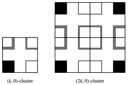
Figure 10. $\square(2k)$ is tiled by the foldings of $\square(k)$.

For $s,t=0,1,\dots,2k-1$,

(4.11) $$v_{s,t}(a+bi)=e^{\pi i(sa+tb)/k},\quad\text{for $a+bi\in S(2k):=\left\{a+bi\mathrel{}\middle|\mathrel{}0\leq a,b\leq 2k-1\right\}$,}$$

give all the eigenfunctions of the torus which is obtained by adding edges between $a$ and $a+(2k-1)i$, and between $bi$ and $2k-1+bi$ for each $a,b=0,1,\dots,2k-1$. The corresponding eigenvalues are given as

(4.12) $$\lambda_{s,t}=\lambda_{s,t}(2k)=4-2\cos\frac{\pi s}{k}-2\cos\frac{\pi t}{k}.$$

Let

$$u_{s,t}:=\sum_{\sigma\in D_{4}}\sigma v_{s,t}\quad\text{and}\quad w_{s,t}:=\sum_{\sigma\in D_{4}}\operatorname{sgn}(\sigma)\sigma v_{s,t}$$

be the projections of $v_{s,t}$ to $\mathcal{U}_{2k}$ and $\mathcal{W}_{2k}$ respectively. Note here that, unlike the $3$-valent case, $u_{s,t}$ and $w_{s,t}$ always lie in the image of $\iota$. Similar computations as in the proof of Lemma 4.3 show that $u_{s,t}\equiv 0$ if and only if $u_{s,t}$ is either

• $u_{s,k}$ for $0\leq s\leq 2k-1$; or

• $u_{k,t}$ for $0\leq t\leq 2k-1$,

and that $w_{s,t}\equiv 0$ if and only if $w_{s,t}$ is one of the following:

• $w_{s,k}$ for $0\leq s\leq 2k-1$;

• $w_{k,t}$ for $0\leq t\leq 2k-1$;

• $w_{s,s}$ for $0\leq s\leq 2k-1$;

• $w_{s,2k-s}$ for $0\leq s\leq 2k-1$.

Moreover a simple computation shows that if both $s$ and $t$ are divisible by $2$, then $u_{s,t}|_{\square(k)}$ is also a $D_{4}$-invariant eigenfunction.

Since $f_{s,t}=u_{s,t}$ or $w_{s,t}$ satisfies

$$f_{s,t}={} f_{t,s}=e^{-\pi is/k}f_{2k-s,t}=e^{-\pi is/k}f_{t,2k-s}$$

$$={} e^{-\pi it/k}f_{2k-t,s}=e^{-\pi it/k}f_{s,2k-t}=e^{-\pi i(s+t)/k}f_{2k-s,2k-t}=e^{-\pi i(s+t)/k}f_{2k-t,2k-s}$$

and therefore

(4.13) $$\left\{u_{s,t}\mathrel{}\middle|\mathrel{}t\leq s\leq k-1,\ 0\leq t\leq k-1\right\}\cup\left\{w_{s,t}\mathrel{}\middle|\mathrel{}t+1\leq s\leq k-1,\ 0\leq t\leq k-1\right\}$$

gives a complete list of the eigenfunctions of $\square(k)$ because its total number is computed as $(k^{2}/2+k/2)+(k^{2}/2-k/2)=k^{2}$.

Theorem 1.1 is now proved similarly as in the $3$-valent case only by noting that the function $S(2k)\ni(s,t)\mapsto\lambda_{s,t}\in[0,8]$ takes value near $0$ (resp. $8$) only near the four corners (resp. the center) of $S(2k)$.

Proofs of (1.3) in Theorem 1.2 and Theorem 1.3.

The same computation as above shows that the projection $u_{s,t}\in\mathcal{U}_{k}$ of $v_{s,t}$ defined on $S(k)$ vanishes if and only if $k$ is even and either

• $u_{s,k/2}$ for $0\leq s\leq k-1$; or

• $u_{k/2,t}$ for $0\leq t\leq k-1$.

Therefore

$$\lambda_{s,s}(k)=4-4\cos\frac{2\pi s}{k}\quad\text{for $0\leq s\leq k-1$ and $s\neq k/2$}$$

are all $D_{4}$-invariant eigenvalues for the $(k,0)$-cluster, and an arbitrary real number in $[0,8]$ is approximated by these values as $k$ tends to infinity, which proves Theorem 1.3.

(4.6) is valid also for a $4$-valent graph, and the inequality (1.3) is obtained by choosing $\lambda=\lambda_{(k-2)/2,(k-2)/2}(k)=4+4\cos(2\pi/k)$ if $k$ is even and $\lambda=\lambda_{(k-1)/2,(k-1)/2}(k)=4+4\cos(\pi/k)$ if $k$ is odd. ∎

5. On the eigenvalues $2$ and $4$ for Goldberg-Coxeter constructions

This section provides proofs of the theorems on multiplicities of eigenvalues $2$ and $4$ stated in Section 1. In the first two subsections, we shall prove Theorems 1.4 and 1.5. As is seen below, a reason for large multiplicities of eigenvalues $2$ and $4$ of $\operatorname{GC}_{2k,0}(X)$ is that the $(2k,0)$-clusters also have large multiplicities of eigenvalues $2$ and $4$. On the other hand, it is considered that the structure of an initial graph $X$ would affect the eigenvalue distribution of its Goldberg-Coxeter constructions. A few remarkable examples shall be provided in Section 5.3, where a proof of Theorem 1.6 is also included.

5.1. The case where $X$ is $3$-valent

From what was mentioned in (1) of Remark 4.2, Theorem 1.4 is an immediate consequence of the following lemma.

Lemma 5.1.

For $k\geq 1$ (resp. $k\geq 2$), the $3$-valent $(2k,0)$-cluster $\triangle(2k)$ has a $D_{3}$-invariant eigenvalue $4$ (resp. $2$), whose multiplicity is at least $\lceil k/2\rceil$ (resp. $\lfloor k/2\rfloor$).

Proof.

For $0\leq s,t<6k$, as is easily proved from a direct computation using (4.4), $\lambda_{s,t}^{+}(6k)$ (resp. $\lambda_{s,t}^{-}(6k)$) takes the value $4$ (resp. $2$) if and only if $s$ and $t$ satisfy either $s=3k$ or $t=3k$ or $s-t=3k$ or $s-t=-3k$. Among (4.9) with $k$ replaced with $2k$, $\lambda_{s,t}^{+}=4$ for, and only for, $s=3k$ and $t=3j$ ($0\leq j<k/2$), and $\lambda_{s,t}^{-}=2$ for, and only for, $s=3k$ and $t=3j$ ($0<j\leq k/2$). All of them are $D_{3}$-invariant by Lemma 4.4. The corresponding $u_{s,t}^{\pm}$’s are linearly independent from the consequence obtained in the proof of Theorem 1.1. ∎

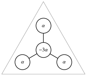
(a) with eigenvalue $4$

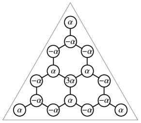
(b) with eigenvalue $2$

Figure 11. $D_{3}$-invariant eigenfunctions

5.2. The case where $X$ is $4$-valent

Similarly as in the $3$-valent case, Theorem 1.5 is a consequence of the following.

Lemma 5.2.

For $k\geq 2$, the $4$-valent $(2k,0)$-cluster $\square(2k)$ has a $D_{4}$-invariant eigenvalue $4$, whose multiplicity is at least $\lceil(k-1)/2\rceil$.

Proof.

It is easily confirmed that $\lambda_{s,t}(4k)=4$ if and only if $s$ and $t$ satisfy either $s+t=2k$ or $s+t=6k$ or $s-t=2k$ or $s-t=-2k$. The number of $u_{s,t}$’s out of (4.13) satisfying $\lambda_{s,t}(4k)=4$ is therefore computed as $\lceil(k-1)/2\rceil$. ∎

5.3. Dependence on the structure of $X$ (only for $3$-valent case)

This subsection provides the proofs of Theorem 1.6, which describes relations between the conditions (F), (CN), (N) and (C) in Section 2.2, and eigenvalues $2$ and $4$ of some $\operatorname{GC}_{k,0}(X)$’s.

Proof of (1) of Theorem 1.6.

Let us take a vertex numbering $V(\operatorname{GC}_{2,0}(X))\rightarrow\{1,2,3\}$ satisfying (N), whose existence is guaranteed by Proposition 2.9. Let $\alpha_{0},\alpha_{1},\alpha_{2}$ and $\alpha_{3}$ be complex numbers satisfying $\alpha_{0}+\alpha_{1}+\alpha_{2}+\alpha_{3}=0$. Then it is easy to see that the function $v\colon V(\operatorname{GC}_{2,0}(X))\rightarrow\mathbb{C}$ which maps a vertex with number $i$ to $\alpha_{i}$ is an eigenfunction of $\Delta_{\operatorname{GC}_{2,0}(X)}$ with eigenvalue $4$. By above reasons, we can find two more eigenfunctions which are linearly independent with $u=u_{\alpha}$ which was obtained in Theorem 1.4 (1); in fact, set $(\alpha_{0},\alpha_{1},\alpha_{2},\alpha_{3})=(0,1,-1,0),(0,1,1,-2)$ for example. ∎

Let us next consider the condition (C). Our assertions are summarized as follows.

Proposition 5.3.

Let $X$ be a $3$-valent plane graph.

1. If $X$ has a vertex coloring satisfying (C-i) and (C-ii), then for any $s\in\mathbb{N}$, $\operatorname{GC}_{2s-1,0}(X)$ has eigenvalue $4$.

2. If $X$ has a vertex coloring satisfying (C-i), (C-ii) and (C-iii), then for any $k\in\mathbb{N}$, both $\operatorname{GC}_{k,0}(X)$ and $\operatorname{GC}_{k,k}(X)$ have eigenvalue $4$ (resp. $2$), whose multiplicity is at least $\lceil k/2\rceil$ (resp. $\lfloor k/2\rfloor$).

Proof.

(1) The function $u\colon V(X)\rightarrow\mathbb{C}$ which maps a black vertex to $-3$ and a white one to $1$ is an eigenfunction of $\Delta_{X}$ with eigenvalue $4$, which proves (1) for $s=1$.

For $s\geq 2$, a quadruplet $\{\triangle(p),\triangle(q_{1}),\triangle(q_{2}),\triangle(q_{3})\}$ of $(2s-1,0)$-clusters, where $p$ is black and $N_{X}(p)=\{q_{1},q_{2},q_{3}\}$ are all white, can be glued with each other to be identified with a $(4s-2,0)$-cluster. On the other hand, it follows from a direct computation that $u_{3(2s-1),0}^{+}\in\mathcal{U}_{3(4s-2)}$ of (4.5) gives a $D_{3}$-invariant eigenfunction on $\triangle(4s-2)$ with the eigenvalue $4$ with the constant boundary value $4$. Therefore $u$ defines an eigenfunction on $\operatorname{GC}_{2s-1,0}(X)$ with eigenvalue $4$, proving (1).

(2) In the argument above to prove the existence $u$ on $\triangle(4s-2)$, if (C-iii) is further satisfied, then any $D_{3}$-invariant eigenfunction on $\triangle(4s-2)$ with eigenvalue $4$ (resp. eigenvalue $2$) gives an eigenfunction on $\operatorname{GC}_{2s-1,0}(X)$ with eigenvalue $4$ (resp. eigenvalue $2$). For exactly the same reason, any $D_{3}$-invariant eigenfunction on $\triangle(4s)$ with eigenvalue $4$ (resp. eigenvalue $2$) gives an eigenfunction $\operatorname{GC}_{2s,0}(X)$ with eigenvalue $4$ (resp. eigenvalue $2$). This and (3) in Examples 2.11 now prove (2). ∎

Proof of (2) of Theorem 1.6.

The assertion is an immediate consequence of Proposition 5.3 and Proposition 2.10. ∎

Acknowledgment

Authors are partially supported by JSPS KAKENHI Grant Number 15K17546, 15H02055, 25400068, 18K03267, 26400067, 17H06465, 17H06466, and 19K03488. This work is also supported by JST CREST Grant Number JPMJCR17J4.

References

- [1] H. S. M. Coxeter. Virus macromolecules and geodesic domes, In A spectrum of mathematics (Essays presented to H. G. Forder), pages 98–107. Auckland Univ. Press, Auckland, 1971.
- [2] D. Cvetković, P. Rowlinson and S. Simić. An introduction to the theory of graph spectra, volume 75 of London Mathematical Society Student Texts. Cambridge University Press, Cambridge, 2010.
-
[3]
G. Davidoff, P. Sarnak and A. Valette.
Elementary number theory, group theory, and Ramanujan graphs,
volume 55 of London Mathematical Society Student Texts.
Cambridge University Press, Cambridge, 2003.
doi:10.1017/CBO9780511615825. -
[4]
M. DeVos, L. Goddyn, B. Mohar, and R. Šámal,
Cayley sum graphs and eigenvalues of -fullerenes,
J. Combin. Theory Ser. B, 99, 358–369, (2009).
doi:10.1016/j.jctb.2008.08.005. - [5] M. Deza and M. Dutour Sikirić. Geometry of chemical graphs: polycycles and two-faced maps, volume 119 of Encyclopedia of Mathematics and its Applications. Cambridge University Press, Cambridge, 2008. doi:10.1017/CBO9780511721311.
-
[6]
M. Dutour and M. Deza.
Goldberg-Coxeter construction for 3- and 4-valent plane graphs.
Electron. J. Combin., 11, R20, (2004).
https://www.combinatorics.org/ojs/index.php/eljc/article/view/v11i1r20. - [7] S. Fisk, Combinatorial structure on triangulations. I. The structure of four colorings. Advances in Math., 11, 326–338, (1973).
- [8] S. Fisk, Combinatorial structures on triangulations. II. Local colorings. Advances in Math., 11, 339–350, (1973).
- [9] S. Fisk, Combinatorial structures on triangulations. III. Coloring with regular polyhedra. Advances in Math., 12, 296–305, (1974).
- [10] S. Fisk, Grötzsh’s Heawood coloring theorem. Advances in Math., 15, 162–163, (1975).
- [11] S. Fisk, Variations on coloring, surfaces and higher-dimensional manifolds. Advances in Math., 25, 226–266, (1977).
- [12] S. Fisk, Geometric coloring theory. Advances in Math., 24, 298–340, (1977).
-
[13]
D. Fujita, Y. Ueda, S. Sato, N. Mizuno, T. Kumasaka, and M. Fujita,
Self-assembly of tetravalent Goldberg polyhedra from 144 small components,
Nature, 540, 563, (2016).
doi:10.1038/nature20771. - [14] H. Fleischner, Eulerian graphs and related topics. Part 1. Vol. 1, volume 45 of Annals of Discrete Mathematics. North-Holland Publishing Co., Amsterdam, 1990.
- [15] M. Goldberg. A class of multi-symmetric polyhedra. Tohoku Mathematical Journal, First Series, 43, 104–108, (1937).
-
[16]
M. D. Horton, D. B. Newland and A. A. Terras.
The contest between the kernels in the Selberg trace formula for the -regular tree.
In The ubiquitous heat kernel, Contemp. Math., 398, 265–293, (2006).
doi:10.1090/conm/398/07492. - [17] G. Hu and W. -Y. Qui, Extended Goldberg polyhedra, MATCH Commun. Math. Comput. Chem., 59, 585–594, (2008).
-
[18]
R. Kaplan, J. Klobusicky, S. Pandey, D. H. Gracias, and G.Menon,
Building Polyhedra by Self-Assembly: Theory and Experiment,
Artificial Life, 20, 409–439, (2014).
doi:10.1162/ARTL_a_00144. - [19] J. A. Kelner, Spectral partitioning, eigenvalue bounds, and circle packings for graphs of bounded genus, SIAM J. Comput., 35, 882–902, (2006).
- [20] J. .A. Kelner, J. R. Lee, G. N. Price and S.-H. Teng, Metric uniformization and spectral bounds for graphs, Geom. Funct. Anal., 21, 1117–1143, (2011).
-
[21]
M. Kotani, H. Naito and T. Omori,
A discrete surface theory,
Comput. Aided Geom. Design, 58, 24–54, (2017).
doi:10.1016/j.cagd.2017.09.002. -
[22]
B. D. McKay.
The expected eigenvalue distribution of a large regular graph.
Linear Algebra Appl., 40, 203–216, (1981).
doi:10.1016/0024-3795(81)90150-6. -
[23]
H. Naito,
Construction of negatively curved cubic carbon crystals via standard realizations,
Springer Proc. Math. Stat., 166, 83–100, (2016).
doi:10.1007/978-4-431-56104-0_5. -
[24]
S. Schein and J. M. Gayed,
Fourth class of convex equilateral polyhedron with polyhedral symmetry related to fullerenes and viruses,
Proc. Nat. Acad. Sci., 111, 29202925, (2014).
doi:10.1073/pnas.1310939111 - [25] D. A. Spielman and S. H. Teng, Spectral partitioning works: planar graphs and finite element meshes, Linear Algebra Appl., 421, 284–305, (2007).