Automatic Processing and Solar Cell Detection in Photovoltaic Electroluminescence Images

Abstract

Electroluminescence (EL) imaging is a powerful and established technique for assessing the quality of photovoltaic (PV) modules, which consist of many electrically connected solar cells arranged in a grid. The analysis of imperfect real-world images requires reliable methods for preprocessing, detection and extraction of the cells. We propose several methods for those tasks, which, however, can be modified to related imaging problems where similar geometric objects need to be detected accurately. Allowing for images taken under difficult outdoor conditions, we present methods to correct for rotation and perspective distortions. The next important step is the extraction of the solar cells of a PV module, for instance to pass them to a procedure to detect and analyze defects on their surface. We propose a method based on specialized Hough transforms, which allows to extract the cells even when the module is surrounded by disturbing background and a fast method based on cumulated sums (CUSUM) change detection to extract the cell area of single-cell mini-module, where the correction of perspective distortion is implicitly done. The methods are highly automatized to allow for big data analyses. Their application to a large database of EL images substantiates that the methods work reliably on a large scale for real-world images. Simulations show that the approach achieves high accuracy, reliability and robustness. This even holds for low contrast images as evaluated by comparing the simulated accuracy for a low and a high contrast image.

and

1 Introduction

The automatic preprocessing of industrial images of objects is an ubiquitous and important task of quality control, in order to prepare object extraction, identification and its assessment as well as comparisons with reference images. For example, this applies to high-resolution imaging technologies to check materials on a microscopic or nano scale, where position and orientation of the sensor and the sample cannot be perfectly controlled. The same issue arises when the object of interest is surrounded by background such as a fluid or gas, or when images are taken in difficult environments, for example under outdoor (or field) conditions. The latter situation motivated and initiated the procedures proposed in this paper.

The preprocessing methods proposed and investigated in this article are tailored to electroluminescence (EL) images of photovoltaic modules and cells, especially when taken under outdoor conditions, but they are applicable to various similar imaging problems, such as the analysis of wafers in CPU production, with appropriate modifications. Nevertheless, in our exposition we will focus on the application to imaging in photovoltaics. The approach presented in this paper has been used to preprocess a large number of EL images collected in a panel-type multi-site study [1], in order to prepare them for further statistical analyses. Tailored multiple regression methods have been proposed by [2] and applied to images preprocessed using the method proposed here. In practice, one often computes certain quality features from the sampled images, and it is even possible to calculate the operating voltage of individual solar cells by EL imaging, [3]. When focusing on the problem to accept or reject a lot of photovoltaic modules (PV modules) based on statistics derived from such images, we refer to [4, 5, 6, 7]. Extensions to two-point inspection schemes have been proposed by [8].

In the photovoltaic industry, imaging is a widely established tool to assess and inspect the quality of PV modules and solar cells. For a general overview and references to established methods aiming at detecting certain defects and issues such as macro-crack detection using anisotropic diffusion as in machine vision, [9] or inspection of electrical contacts, [10], we refer to [11]. EL is one of the most established imaging technologies. It allows a microscopic view into the crystalline cell material and therefore allows to detect faults such as micro cracks, cell breaks or interconnect and soldering flaws, which are usually invisible otherwise, since they are only in effect when the photovoltaic effect is active. EL inverts that photovoltaic effect and allows to image the spatial distribution minority carrier diffusion length, [12]: If a solar cell is supplied by a DC current, radiative recombination occurs and emits photons (i.e. luminescence), which can be captured by a charge coupled device (CCD) camera that is sensitive to the relevant spectrum. Here, long exposure times are required, such that even infinitesimal movements of the camera or the PV module, for example due to wind, vibrancy or shocks, may lead to reduce image sharpness and quality.

Despite the progress, the evaluation of an EL image is usually based on expert knowledge only, [13]. This is mainly due to the lack of appropriate computerized, automatic methods for image processing and advanced image analysis, which requires accurate detection of the relevant cell areas in an image, in order to allow sound statistical analyses of defect. Otherwise, even simple statistical measures such as the percentage of low performing cell area can not be determined, and difference images will show artifacts leading to false detections. These issues, which are of particular relevance for outdoor imaging, call for tailor-made preprocessing methods as proposed in this paper.

When images are collected under field conditions, the required outdoor acquisition procedure leads to several problems that are usually not present in a lab environment. In brief, the process is as follows: First, each PV module is disconnected from the grid. Then, either it is unmounted and carried to a mobile lab or a frame is mounted, which holds the camera and protective curtains to shield the module from external light sources and allow for long-exposure imaging. That procedure is highly sensitive to mechanical deficiencies and stress (incorrect mounting of the frame, imperfect positioning of the camera, vibrancy due to wind, shocks, residual external light etc.) resulting in several image processing problems. Firstly, the module is incorrectly shown on the image, as it can be rotated in all three dimensions, such that it is neither parallel to the camera’s sensor nor its center coincides with the center of the sensor. Secondly, unlike images taken in a laboratory where a fixed and calibrated environment is used, the module’s position differs from image to image. See examples of typical EL images in Section 7.

In this paper, we discuss novel methods that allow to correct for rotation and perspective distortions, to estimate the boundaries of the PV module and to extract all PV cells, which are the relevant areas where the photovoltaic effect occurs. To the best of our knowledge, there is no published method for those problems. One could try to apply methods from machine vision and learning, [14, 15], especially deep learning neural networks which allow to approximate square integrable [16]. For image processing and analysis, convolutional layers are used to extract local information which is processed in later layers to detect geometrical shapes. The trained deep learner is then used as a surrogate model for the unknown optimal classification function and approximates the latter under weak conditions, see [17]. Recent studies, e.g. [18], provided evidence that image classification by such deep learners can be improved by data augmentation or denoising prior to classification. But such approaches, especially data augmentation to deal with noise (see [18, Sec. 6]), require a large learning sample with known - manually determined - correct positions of the solar cells. For the problem at hand this is not feasible. One could also draw on methods developed for the detection of quadrilateral documents in images, see [19] and the references therein. The detection of solar cells in EL images differs in that the number of quadrilateral areas is known and fixed, whereas in document processing either one quadrilateral is determined or, when aiming at the detection of paragraphs etc., it is estimated. Hence the number of detected areas and their relative position may severely depend on the quality of the image. Contrary, the problem studied here is different and our approach makes use of the specific structure and always extracts the right number of areas.

In our approach, we rely on two basic approaches. Firstly, we use the Hough transform, a general approach to locate objects in images, see the review [20]. We adopt and specialize it to the specific case of EL images of PV modules and combine it with statistical robust regression as well as a physical knowledge about optical distortions, namely rotation and perspective distortion. In practice, a further issue arises, namely radial distortion caused by the camera’s lens. There are fairly standard methods to correct for it. For details we refer to [21]. In practice, it is, however, not always possible to correct for this distortion, and therefore we propose preprocessing methods that are to some extent robust with respect to this issue. The second approach applies the CUSUM change-point estimator, see [22], to detect the boundaries of a solar cell. The CUSUM estimator is the Likelihood estimator for independent Gaussian data assuming common means before and after the change. It can also be interpreted as optimally fitting a model where it is assumed that there are exactly two different line segments (foreground = cell area and background), which are separated by the change-points. To the best of our knowledge, the application of that approach to the problem of detecting solar cells in PV modules has not been studied yet.

We discuss two preprocessing work-flows. The first one applies the tasks of rotation correction, perspective correction and cell extraction in a sequential way. It is especially suited for PV modules, which consist of many solar cells. The second approach is a simplified and fast procedure, mainly designed for one-cell modules, which extracts the cell area from the raw image and then applies an appropriate transformation to output a rectangular shaped image of the cell area.

The paper is organized as follows. Section 2 reviews the Hough transform often used to detect lines or, more generally, parametric curves. In Section 3, we describe a method that allows to correct for the rotation of a PV module. Section 4 discusses a method for the correction of perspective distortion. In Section 5, we consider a specialized Hough transform and propose a method for identifying the location of a PV module and its cells, such that they can be extracted from the image. The simplified fast procedure for one-cell modules is presented in Section 6. Lastly, Section 7 applies the methods and algorithms to real images.

2 Hough Transform

The Hough transform is a technique to detect objects such as lines or circles in images, see [20]. It is widely known and used in computer vision applications, [23, 24]. For its efficient computation, several algorithms have been developed, see [25]. It has also been extended to identify parametric curves as discussed and applied in [26].

As a preparation of the proposed algorithms detailed in the subsequent sections and to introduce required notation, we give a brief review of a generic Hough transform. The Hough transform method is applied to a binary image, for example obtained by thresholding a gray scale image. We consider a binary image as a subset $\Omega\subset\mathcal{D}$, where $\mathcal{D}$ is a finite subset of $\mathbb{N}^{2}$ and $\mathbb{N}$ denote the natural numbers. Each element $\omega\in\Omega$ corresponds to the coordinates of a non-zero pixel of binary image.

We call $\mathcal{H}$ a Hough space or Hough domain, if its elements are parameters representing a curve of interest. For example, if $h=(a,b)\in\mathcal{H}$ is a two-dimensional vector, it represents a line, $y=ax+b$, with intercept $b$ and slope $a$ in the image $\Omega$.

The Hough Transform is defined as a mapping which assigns to each coordinate $x\in\mathcal{D}$ a set $H_{x}$ of curves that go through the point, that is a subset of $\mathcal{H}$,

$$\mathcal{P}:\mathcal{D}\to 2^{\mathcal{H}},\mathcal{P}(x)=H_{x}.$$

where $2^{\mathcal{H}}$ is the powerset of $\mathcal{H}$. In case of the Hough line transform, we assign a set of lines going through the point $x$.

For a given image we are interested in identifying a single or several parameters of the Hough space, namely those which should be regarded as curves (or lines) present in the image. The identification of those elements in the Hough space is achieved by solving the following optimization problem.

Let $R$ be a positive number and $B_{R}(h)$ be a neighbourhood of a point $h$ in the space $\mathcal{H}$. Then, the optimization problem is given by

$$\sum\limits_{x\in\Omega}\mathds{1}\left\{B_{R}(h)\cap\mathcal{P}(x)\neq\emptyset\right\}\to\max\limits_{h\in\mathcal{H}}.$$ (1)

Here $\mathds{1}\{A\}$ is equal to $1$, if the expression $A$ is true, and $0$ otherwise.

The neighbourhood $B_{R}(h)$ is usually selected to be an Euclidean ball with radius $R$. Its role is to control the accuracy of the method in finding a curve. Points of the image which are in the neighbourhood are still regarded as lying on the parametric curve given by $h$. One is interested in a global optimum of (1) when searching for a unique curve. Finding multiple local maxima corresponds to the detection of multiple curves.

The optimization problem (1) is solved by using Algorithm 1.

1Select a grid of point in the space $\mathcal{H}$. Associate to each grid point a counter;

2 For each non-zero pixel location $x\in\Omega$ of the binary image evaluate the Hough transform $H_{x}=\mathcal{P}(x)$;

3 For each coordinate $h\in H_{x}$ increment its associated counter;

The result is evaluated by identifying the grid points with the maximal counter value and those where local maxima are present.

Algorithm 1 Hough optimisation algorithm

3 Rotation distortion correction

The procedure to correct for rotation of a PV module in an EL image is pursued by definining an objective function that attains its maximum when the PV module is correctly positioned in the image. That objective function uses the fact that after the optimal rotation the horizontal and vertical lines present in the PV module induce a pattern in the row and column sums.

Formally, let $I$ be a gray scale image, i.e. a function $I:\{1,\ldots,W\}\times\{1,\ldots,H\}\to\mathbb{R}$, where $H$ is the height and $W$ is the width of the image $I$. Define the following two vectors $R^{I}\in\mathbb{R}^{H}$, $C^{I}\in\mathbb{R}^{W}$:

$$R^{I}_{j}=\sum\limits_{i=1}^{W}I(i,j),\quad\text{for }j\in\{1,\ldots,H\},$$

$$C^{I}_{i}=\sum\limits_{j=1}^{H}I(i,j),\quad\text{for }i\in\{1,\ldots,W\}.$$

$R^{I}$ are the column sums of the pixel values and $C^{I}$ are the row sums.

A PV module is correctly positioned in an EL image when all grid lines of the PV module are parallel to the edges of the image. In that case, since the grid lines are darker than the active crystalline area, we would then observe negative peaks in the vectors $R^{I}$ and $C^{I}$. However, when a PV module is rotated then the pixels corresponding to each grid line appear in different coordinates of the vectors $R^{I}$ and $C_{I}$, and hence, no negative peaks are present in $R_{I}$ and $C_{I}$. Therefore, identifying the optimal rotation angle (i.e. when vectors $R^{I}$ and $C^{I}$ contain largest peaks) can be done by maximising variances of the vectors $R^{I}$ and $C^{I}$.

Define $T_{\alpha}(I)$ to be an operator that rotates the image $I$ by the angle $\alpha$ around the image centre. Then, the objective function $f$ is defined by

$$f(T_{\alpha}(I))\coloneqq\mathrm{sd}(R^{T_{\alpha}(I)})+\mathrm{sd}(C^{T_{\alpha}(I)}),$$

where $\mathrm{sd}$ is the sample standard deviation of a vector, i.e., for $x=(x_{1},\dots,x_{n})^{\prime}\in\mathbb{R}^{n}$

$$\mathrm{sd}(x)=\sqrt{\frac{1}{n}\sum\limits_{i=1}^{n}(x_{i}-\bar{x})^{2}},$$

and $\bar{x}$ is the sample mean. In order to correct for the PV module rotation, we solve the following optimization problem

$$f(T_{\alpha}(I))\to\max_{\alpha\in[-\pi/4,\pi/4]}.$$ (2)

The optimization problem (2) is solved with a simple golden section optimisation algorithm (see [27]), as it does not require any additional assumptions on an image $I$ or the function $f$. The golden section algorithm is given in Algorithm 2.

1Let $f$ be an objective function to be maximised on an interval $[a,b]$. Evaluate $f$ at three probe points $a$, $b$ and $x_{0}$, where $x_{0}$ is the smallest of the two points satisfying the golden-ratio relation $\frac{b-a}{b-x_{0}}=\frac{b-x_{0}}{x_{0}-a}$.

2 Evaluate $f$ at the second golden-ratio point $x_{1}$.

3 By comparing four evaluated function values select either the interval $[a,x_{1}]$ or $[x_{0},b]$ to be a new search interval.

Repeat Step 2 until the interval length is smaller than a selected $\varepsilon$. The golden-ratio choice of the probe points guarantees that the three probe points in the new interval also satisfies the golden ratio relation. Therefore, at each step only a single additional function evaluation is performed.

Algorithm 2 The golden-section optimisation algorithm

Observe that the algorithm does not require a preprocessing step to detect the edges, which would increase the computational burden. The algorithm can be applied directly to an EL image.

To summarise, the steps of the PV module rotation correction algorithm are given in Algorithm 3.

1Solve optimization problem (2) using the golden section algorithm (Algorithm 2) and obtain the optimal rotation angle $\alpha_{0}$;

Rotate the image by the angle $\alpha_{0}$.

Algorithm 3 PV module rotation correction

4 Perspective distortion correction

The module rotation transformation discussed in the previous section models a 2-dimensional rotation of a PV module in an EL image; it rotates the optical image of the module on the camera’s sensor. However, a PV module can be rotated in all three dimensions which results in a so-called perspective distortion. Physically that distortion occurs when a PV module surface is not located perpendicular to the focus line of a camera. In this section, we present a method to correct for this type of distortion. As a result, the image is transformed in such a way that all PV module grid lines are parallel to the edges of an EL image.

Correction for perspective distortion is a common subject in image processing (see [28]). In most cases, those algorithms employ easily detectable markers on an image and use their coordinates to estimate the perspective distortion parameters. In our application, placing some markers on PV module is not feasible, and therefore, we need to develop an alternative approach.

The perspective distortion is physically modelled by 8 parameters (see [29]). It preserves straight lines. Therefore, the grid lines of the PV module appear as straight (though not necessarily parallel) lines in an EL image.

In order to correct for perspective distortion, we could follow the same strategy as we use for the correction of a module rotation, see Section 3. However, the resulting optimization problem is more complex as it contains $8$ parameters. Numerical studies indicated that the formulated objective function often has local minima that do not satisfy our objective, which impede its application in practice.

Therefore, our strategy of correction for perspective distortion is as follows. We estimate grid lines using the Hough line transform and use them to estimate the perspective distortion parameters. Note that it suffices to known two vertical and two horizontal lines to determine the perspective parameters. Our estimator, however, incorporates all detected grid lines. In this way, the influence of incorrectly detected lines is reduced and the method is robust against this type of disturbance.

In order to apply the Hough line transform, we need to obtain a binary image. Instead of simple thresholding of a given image, we use specific versions of the USAN edge detection algorithm, [30, 31, 32] in order to improve the accuracy of the detection. The USAN approach aims at reproducing edges and simultaneously smoothes homogeneous areas, which increases the signal-to-noise ratio and leads to improved line detection. A further important motivation for choosing the USAN edge detector is that it can be designed to output thick edges. This is beneficial when the grid lines do not appear as straight lines, e.g. due to the radial distortion effect or low contrast. In this way the proposed method is robust with respect to radial distortion.

We apply the USAN edge detection twice with two different kernels. Firstly, we apply the edge detector with vertically positioned rectangular kernel, so that its sensitivity with respect to vertically positioned edges is high, whereas its sensitivity to detect horizontal lines is low. Secondly, we apply the USAN edge detector with horizontally positioned rectangular kernel, which is tuned to detect horizontally positioned edges. As a result, we obtain two binary images: one image with horizontal and another one with vertical edges.

The Hough line transform is then applied to the resulting edge images. The binary image with horizontal edges is used to detect the horizontal grid lines, whereas the second image with vertical edges yields the vertical grid lines. Recall that the result of the Hough line transform is a collection of lines. In order to avoid non-grid line detections, we remove those vertical and horizontal lines which have slopes and angles, respectively, lying outside preselected intervals.

At this stage of the procedure we obtain two data sets consisting of the detected horizontal and vertical lines. For each of those data sets linear regressions are conducted, where the independent variable is the ordinate of a vertical lines (or an abscissa in case of horizontal lines) and the dependent variable is the corresponding line slope angle. For details and illustrations we refer to [33]. As a result, we obtain estimates of the angle of a vertical (horizontal) grid line’s slope as a function of $x$ ($y$).

It remains to estimate the perspective distortion parameters from those functions. Obviously, it is sufficient to specify the coordinates of two quadrangles (see Figure 1). For that construction fix 4 points $M$, $N$, $P$ and $Q$. The first quadrangle is the square $A^{\prime}B^{\prime}C^{\prime}D^{\prime}$. The second quadrangle is obtained by considering the intersection of the following four lines. The first line is the line passing through the point $M$ with a slope equal to the value predicted by the simple linear regression for vertical lines, evaluated at the ordinate of the point $M$. The second line is the line passing through the point $N$ with a slope equal to the predicted value resulting from the simple linear regression for horizontal lines, evaluated at the abscissa of the point $N$. The remaining lines corresponding to the points $P$ and $Q$ are calculated analogously.

The resulting coordinates of the two rectangles are now used to feed the perspective distortion procedures. In our implementation we use the corresponding function from the ImageMagick library [34].

Figure 1: Scheme of correcting the rectangular

The method of perspective distortion correction discussed here combines USAN edge detection and Hough line transform sub-procedures. These procedures have several tuning parameters. The question arises as to how one should select those parameters. In order to be able to use one set of tuning parameters for every EL image, we standardize the image (subtract mean and divide by standard deviation of pixel value intensities) and select USAN edge detector and Hough line transform parameters manually by trial-and-error.

We summarise the perspective distortion correction procedure in Algorithm 4.

1Standardise image;

2 Apply vertical and horizontal USAN edge detection yielding $I_{v}$ and $I_{h}$;

3 Apply Hough line transform to the binary images $I_{v}$ and $I_{h}$;

4 Threshold vertical and horizontal lines with respect to the allowed slope angle intervals;

5 Compute two simple linear regressions for the vertical and horizontal slopes;

6 Use these linear regressions to compute the coordinates of quadrangles vertices in Figure 1;

Apply perspective distortion transformation using the computed quadrangles vertices.

Algorithm 4 PV module perspective distortion correction

5 Cell detection

In this section we describe a specialized version of the Hough transform discussed in Section 2, which aims at identifying the location of a PV-module and all solar cells in an EL image. Whereas the Hough transform is often used to detect small, localized objects of given shape like circles, [20], here we develop a Hough transform to identify a complex structure (the module and its grid line structure separating the cells) stretched out over a large part of the image. We use the Hough transform to seek that pattern.

Recall from our discussion above that parallel lines may be bent in a real EL image, due to the effect of radial distortion. Further, a PV module is usually rotated and not positioned perpendicular to the camera’s focus axis. The latter results in rotation and perspective distortions. Although it could be possible to design an algorithm based on the Hough transform that takes into account the radial, the rotation and the perspective distortion parameters simultaneously, the resulting model contains too many parameters and the Hough transform optimization problem becomes hard to compute.

In the first pre-processing step, we first apply the radial distortion correction procedure as described in [21], and the rotation and perspective distortion correction procedures discussed in the previous sections. Thus, the problem to identify the positions of the module and its cells in the image can be reduced to finding the pattern of grid lines, i.e. a fixed number of vertical and horizontal lines in the EL image. The problem can be split into two problems by separately detecting the vertical and horizontal lines.

Since the physical dimensions of a PV module are known, and so are the distances between the grid lines relative to the size of module, the problem of cell detection can be formulated as follows: detect $n$ parallel lines (see Figure 2) separated by intervals that are equal to $\Delta_{0},\Delta_{2},\ldots,\Delta_{n-1}$, where the value $n\in\mathbb{N}$ and the quantities

$$\delta_{l}\coloneqq\sum_{k=0}^{l}\frac{\Delta_{k}}{\sum_{j}{\Delta_{j}}},\quad l\in\{0,\ldots,n-1\}$$

are given.

Figure 2: The (relative) distances between the grid lines of a PV-module are known. This information can be used for their detection in an EL image.

In order to formulate the Hough transform method for the detection of those kinds of patterns, we need to define the Hough space and Hough transform. The domain is $\mathcal{D}=\{1,\ldots,W\}\times\{1,\ldots,H\}$, where $W$ and $H$ are width and height of the image. A binary image can be represented as $\Omega\subset\mathcal{D}$. Now define the Hough space as $\mathcal{H}=\{1,\ldots,W\}^{\times 2}$. For $h=(a,b)^{T}\in\mathcal{H}$ the first coordinate defines the position of the first line and the second coordinate defines the position of the last line in the pattern. Locations of other lines can be easily computed, because the relative distances between them are known. The Hough transform map $\mathcal{P}$ is defined as follows:

$$\mathcal{P}(x,y)\coloneqq\bigcup\limits_{l=0}^{n-1}\left\{(a,b)\in\mathcal{H}:x=a+\delta_{l}(b-a)\right\}.$$

Let us note, firstly, that the map $\mathcal{P}$ does not depend on the second coordinate $y$. Therefore, the objective function can be rewritten in the form

$$\sum\limits_{(x,y)\in\Omega}\mathds{1}\left\{B_{R}(h)\cap\mathcal{P}(x,y)\neq\emptyset\right\}=$$

$$\sum\limits_{(x,y)\in\Omega}y\mathds{1}\left\{B_{R}(h)\cap\mathcal{P}(x,y)\neq\emptyset\right\}\to\max_{h\in\mathcal{H}}.$$ (3)

The above problem can also be reformulated as follows. Instead of considering a binary image $\Omega$, we consider a vector of length $W$ consisting of tuples with an abscissa coordinate and the sum of pixel values of the column of the image corresponding to that abscissa coordinate. This means, $\bar{\Omega}=\left\{(x,y)^{T}\in\{1,\ldots,W\}\times\{1,\ldots,H\}\right\}$, where $y$ is the $x$-th column sum of the values of the binary image. The Hough transform map is the same as in the optimization problem given in (3). By solving the resulting optimization problem,we identify $n$ peaks in the series $\bar{\Omega}$ with fixed relative distances between them. An example of such a series of column means and its pattern of local peaks is shown in Figure 3.

Figure 3: The column sums indicate the grid lines.

A further improvement can be achieved by adding additional constraints on the parameter $h\in\mathcal{H}$. Firstly, it is reasonable to assume that there are two constants $L,U$ such that $L\leq h_{2}-h_{1}\leq U$, where $h_{1}$ and $h_{2}$ are the two coordinates of the vector $h$. Those constraints mean that a module has width more than $L$ and less than $U$ pixels. Secondly, we assume that the PV module is located completely inside an EL image, such that $0\leq h_{1},h_{2}\leq W$.

Hence, the final formulation of optimization problem is given by

$$\begin{split}\sum\limits_{(x,y)^{T}\in\Omega}y\mathds{1}(B_{R}(h)\cap\mathcal{P}(x,y)\neq\emptyset)\to\max_{h\in\mathcal{H}}\\ L\leq h_{2}-h_{1}\leq U,\quad 0\leq h_{1},h_{2}\leq W,\end{split}$$ (4)

where $R$ is a method parameter. The parameter $R$ determines the accuracy of the method by allowing a pattern to fit imprecisely inside a binary image in the following sense: The distance between each line and its true position can be up to $R$ pixels. In our application it turned out that even small values of $R$ (we chose $R=5$) give accurate results. Further, allowing for such an imprecision automatically provides robustness of the method, when the pattern lines are slightly distorted by, for example, uncorrected radial distortion.

We solve the optimization problem using the method described in Section 2. The most time-consuming step in this optimization is the evaluation of the transformation map $\mathcal{P}$. For the present setting, this evaluation boils down to solving a system of linear inequalities. We list these inequalities in Appendix A.

In order to apply the Hough Transform approach, introduced above for an EL image, we need to preprocess it to obtain a binary image. For the cell detection method we use the well-known Canny edge detection algorithm implemented in the OpenCV library [35].

The cell detection method uses other preprocessing method that require tuning parameters. We choose those tuning parameters in the same fashion as in Section 4 for perspective distortion correction method, namely, by standardizing the image and choosing parameters manually.

We summarise the presented method in Algorithm 5.

1Standardise image;

2 For a given module type, compute from physical characteristic $\delta_{l}$ for vertical and horizontal grid lines;

3 Apply Canny edge transformation to obtain a binary image;

4 Perform the Hough Transform optimization twice with the selected accuracy parameter $R$ for vertical and horizontal grid lines;

Cut the PV cells according to the detected grid lines.

Algorithm 5 PV module cell detection

6 One-Cell-Extraction Based on Change Point Estimation

In some cases, an image only contains one cell, for example when so-called mini modules are used. Such mini-modules are commonly used in photovoltaic research and development, in order to test new technologies. In this case, the problem breaks down to the detection of the cell boundaries to remove the background. Usually, this will result in a quadrilateral due to the effects discussed in Sections 3 and 4. We propose to correct for this by applying a mapping which maps a quadrilateral to a rectangle of arbitrary pixel resolution. In this way, we obtain a standardized cell image.

For the task of cell identification, one can use the following simplified procedure which detects separately the four corners and then extracts the associated quadrilateral representing the relevant cell area. It uses minimal a priori knowledge about the location of the cell corners in the sense that one provides four points which are near the corners but closer to the center of the image, so that the associated horizontal and vertical lines cross the boundaries of the cell. We use the pixel values on those lines to detect the boundary, which is represented as a change-point where the (average) value of the pixels changes. This observation can be exploited and motivates to use change-point estimation methods. It is worth mentioning that this approach also works, if one needs to extract the smallest quadrilateral whose sides are boundaries of the object of interest, e.g. if the corners are rounded as it is the case for the mini-modules, see Figure 7, such that they are more or less virtual.

The details are as follows. Assume that the upper left corner of the image with resolution $n\times m$ corresponds to the origin $(0,0)$ of the image. To detect the true coordinates $(x_{0,true},y_{0,true})$ of the upper left corner we fix a vertical $y$-coordinate $y_{0}$ provided by the user, which is known to be larger than the $y$-coordinate, $y_{0,true}$, of the corner. The gray values of the pixels located on the horizontal row $(x,y_{0}),x=0,\ldots,n-1$, define a sequence $X_{0},\ldots,X_{n-1}$, which has a change in the mean, namely at the index which corresponds to the pixel where the boundary of the cell area is located. This change-point can be detected by applying the cumulated sum (CUSUM) change-point estimator, which is described below. This CUSUM detector outputs $x_{c}$. Next we take some horizontal $x$-coordinate $x_{0}$, provided by the user, being larger than the $x$-coordinate, $x_{0,true}$, of the corner. Extract the pixel values located on the vertical row (line) $(x_{0},y),y=0,\ldots,m-1$, and denote them $Y_{0},\ldots,Y_{m-1}$. This sequence has a change-point at the $y$-coordinate of the boundary, and again we can detect it by applying the CUSUM detector. It outputs $y_{c}$. The resulting estimate of the coordinates of the upper left corner is $(x_{c},y_{c})$. In a similar way, we can detect the remaining corners.

The CUSUM approach to estimate the change-point works as follows: Assume it is fed with a sequence, $X_{0},\ldots,X_{n-1}$, assumed to be a random sample with finite variance, which has a change in its mean at $q$. This means, we assume that

$$E(X_{i})=\mu_{0},\quad i<q$$

and

$$E(X_{i})=\mu_{1},\quad i\geq q.$$

Here $\mu_{0}$ denotes the mean of the background pixels and $\mu_{1}$ the mean of the cell area. This model is justified as a kind of a first order approximation for practical purposes, assuming that the distance between the average of the background pixels and the average of the cell area pixels is much larger than the variation of the pixels within each of those two segments. It can be shown that the change-point can be consistently estimated by minimizing the objective function

$$RSS(k)=\sum_{i<k}(X_{i}-X_{1:k})^{2}+\sum_{i\geq k}(X_{i}-X_{k:n})^{2}$$

where $X_{1:k}$ denotes the arithmetic mean of the first $k$ observations and $X_{k:n}$ the arithmetic mean of the remaining data points. This means, we minimize the residual sum of squares calculated under the assumption that the change-point is $k$; then the mean of the pre-change observations is estimated by $X_{k:n}$ and the mean of observations after the change is estimated by $X_{k:n}$. The term $\sum_{i<k}(X_{i}-X_{1:k})^{2}$ arising in $RSS(k)$ is a measure of the variation of the background pixels, as it is $k$ times the sample variance of those values. Analogously, the second term in $RSS(k)$ is $(n-k)$ times the sample variance of cell area pixels. By minimizing $RSS(k)$ we select the best fitting model given the data, and any value $k^{*}$ minimizing $RSS(k)$ is optimal in this sense. For independent normal observations this method is the Maximum Likelihood estimator, see [22].

The output of the above algorithm is in general a quadrilateral. Let us denote the coordinates of its corners by $(x_{1},y_{1}),\dots,(x_{4},y_{4})$, ordered as upper left, upper right, lower left and lower right. Suppose that we want to output an image of resolution $W\times H$. Then the pixel at location $(x,y)$ of the output image is set to the value of the pixel $(x^{\prime},y^{\prime})$ with $x^{\prime}$ the largest integer smaller or equal to
$(1-y^{*})x_{1}+y^{*}x_{3}+x^{*}((1-y^{*})(x_{2}-x_{1})+y^{*}(x_{4}-x_{3}))$ and $y^{\prime}$ the largest integer smaller or equal to
$(1-x^{*})y_{1}+x^{*}y_{2}+y^{*}((1-x^{*})(y_{3}-y_{1})+x^{*}(y_{4}-y_{3}))$. where $x^{*}=x/W$ and $y^{*}=y/H$. This transformation maps the quadrilateral to the target rectangle and interpolates in between.

7 Application and Simulations

In this section, we apply the proposed methods to real EL images and report about extensive computer simulations. The simulations study the accuracy of the preprocessing method discussed in Sections 3 - 5, where errors propagated through the stages may aggregate. In a first Monte-Carlo study we sample from our database of real EL images and, for each sampled image, simulate distortions due to rotation, perspective and shift. In a second computer simulation we illustrate the sensitivity with respect to image quality in the sense of contrast. Here, for two selected real EL images of low and high contrast the accuracy of the preprocessing work-flow is simulated.

7.1 Application

We apply our methods to a collection of approximately 2000 EL images. Those images were collected under outdoor (field) conditions in several solar parks. They are taken with a special EL camera that is able to capture the emitted light spectrum from a PV module. The images are stored in a JPEG format and have resolution of approximately $4200\times 2800$ pixels.

Figure 4 shows the output (right image) of the rotation distortion correction method applied to an EL image (right image). Note that the method outputs a rotated image where all vertical grid lines are parallel to the image edges. Among 2000 EL images in our data set there were no images founds, for which the method did not perform visually correctly. However, as one can observe in Figure 4, the horizontal grid lines are not yet perfectly parallel to the edges of the image due to the perspective distortion.

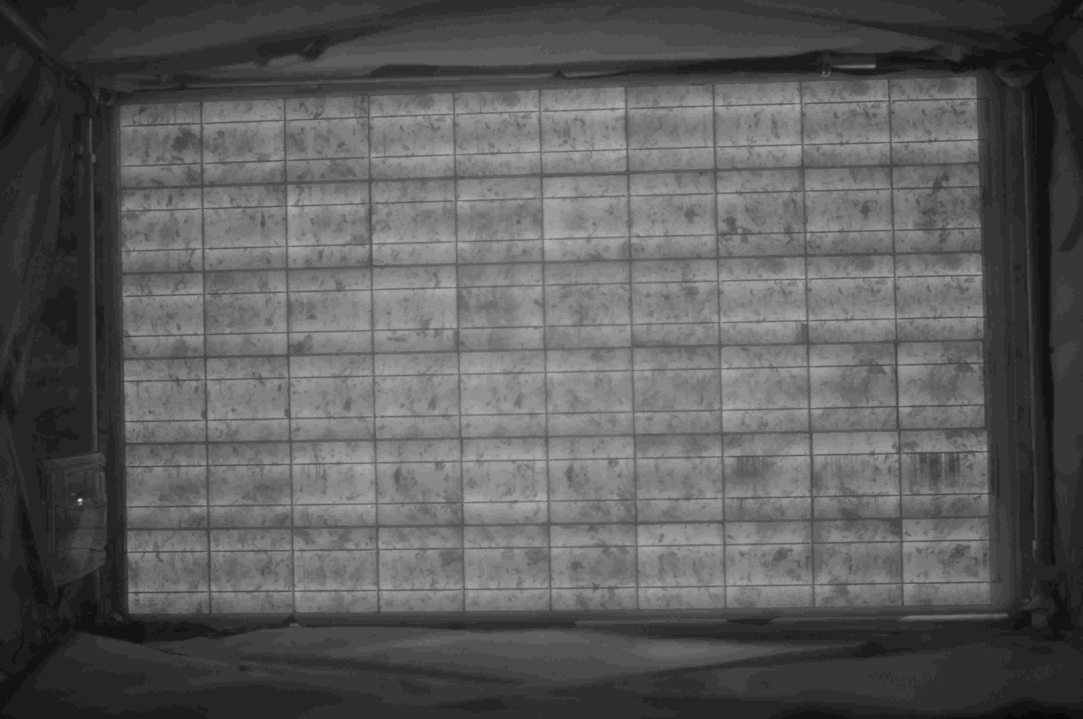
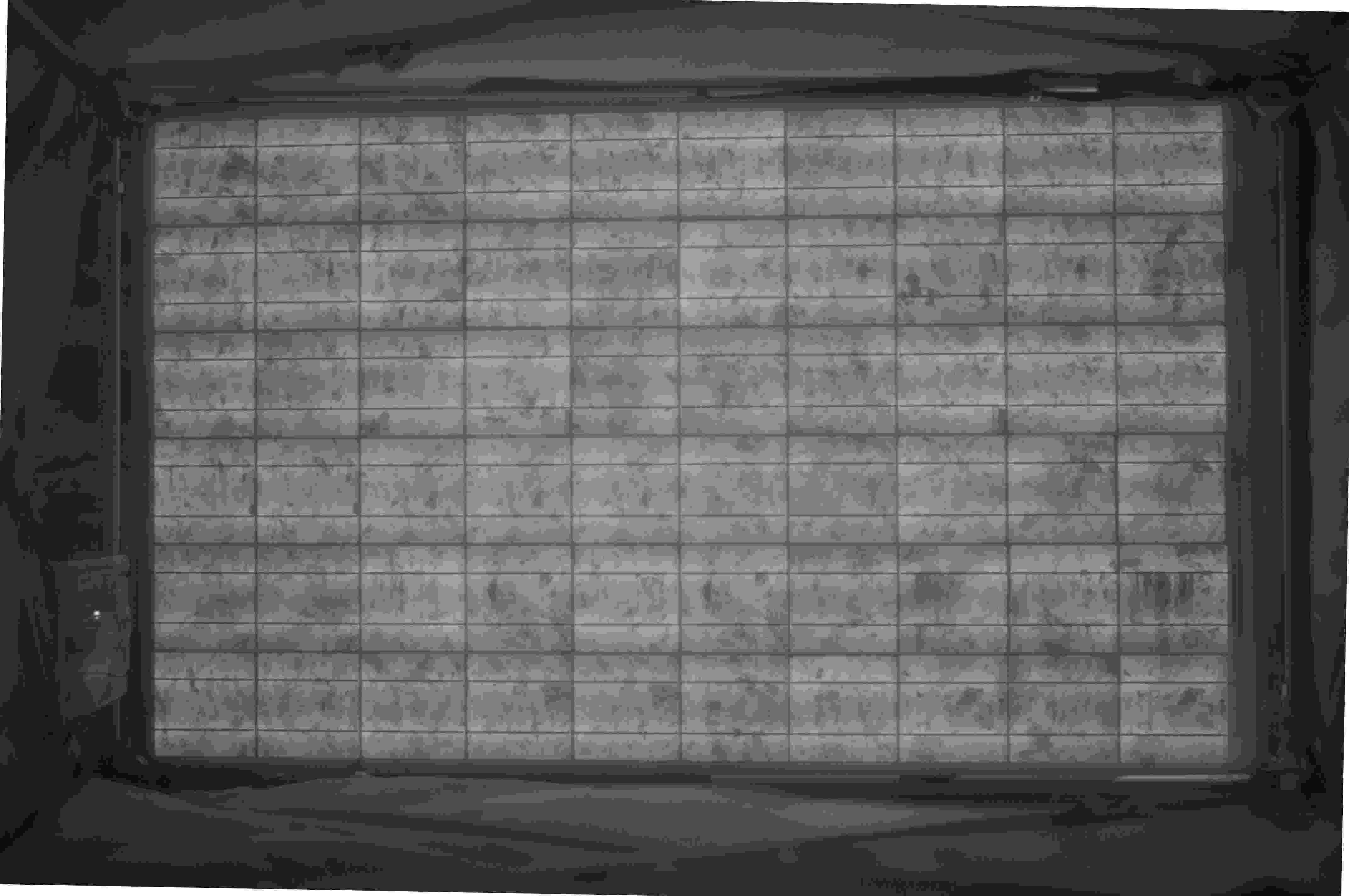
Figure 4: An example of applying rotation correction algorithm. The left image is the original EL image. The right image is the method output.

The application of the perspective distortion correction method is illustrated in Figure 5. The white grid lines are added to assist the visual verification of the achieved distortion correction. Among the 2000 EL images we analyzed, there are only a few images for which the method did not work correctly, since only one vertical or horizontal line was detected, which is not sufficient to estimate the perspective distortion parameters.

The perspective distortion correction method relies on image processing sub-procedures that have several tuning parameters. The USAN edge detector has three parameters and we select them to be equal $H=5$, $h=3$ and $p=0.4$ (see notations in [30]). The Hough Line Transform we use has two parameters: a line threshold equals $50$ and the maximum gap between points forming a line equals $75$.

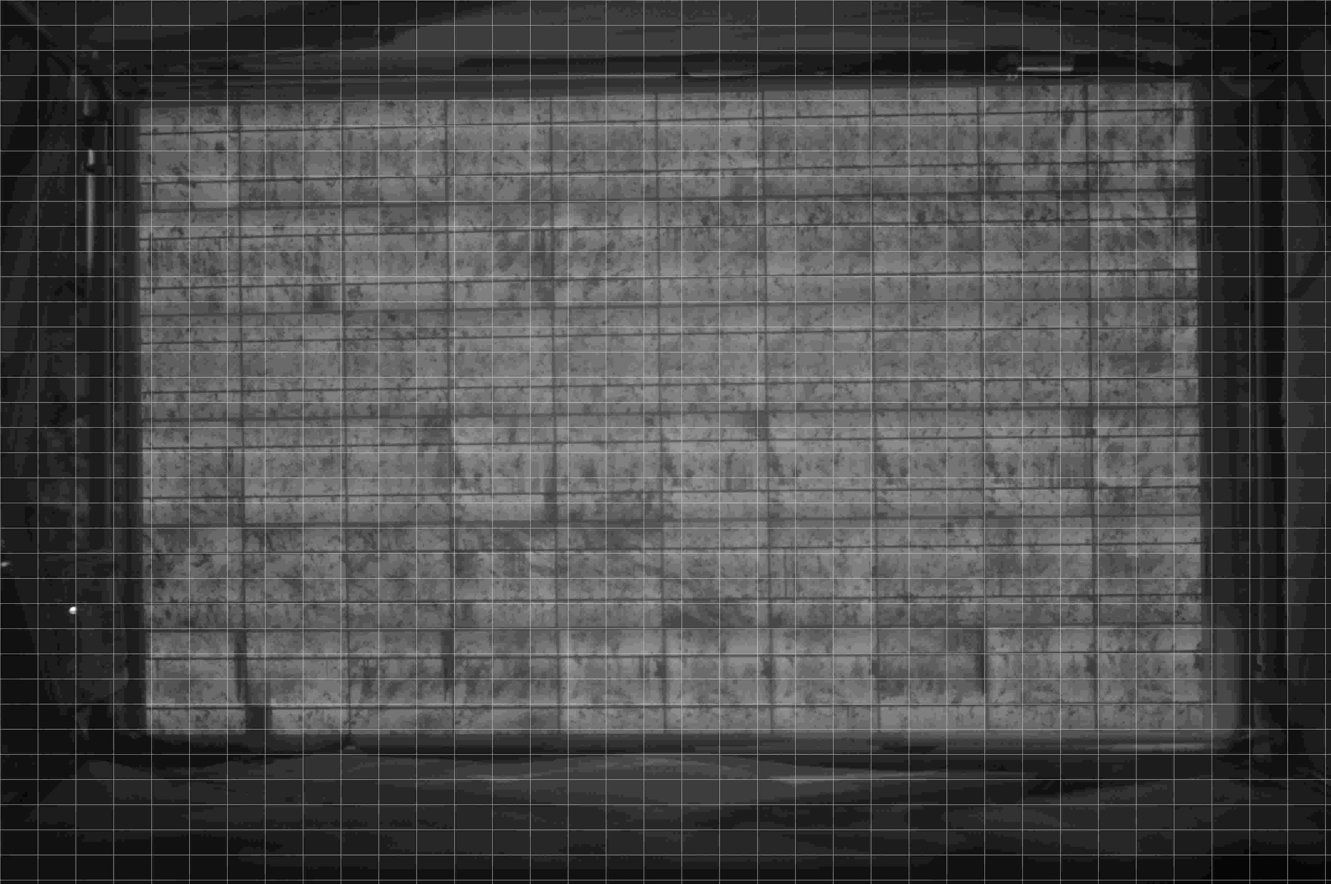
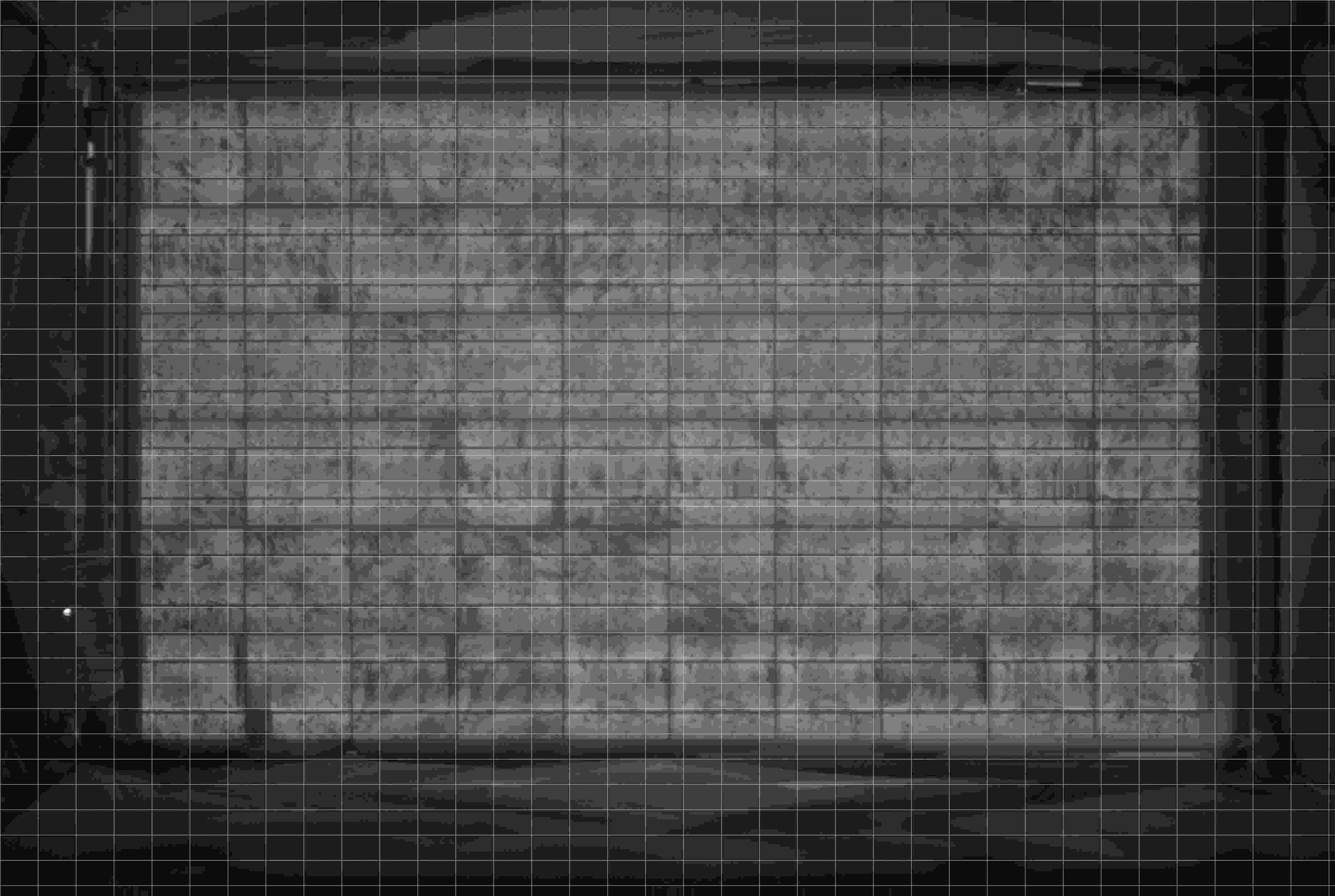
Figure 5: Outdoor EL images are affected by perspective distortion (left image), which needs to be corrected in the presence of possibly disturbing background. The right image shows the output of the proposed method. The white grid lines are added to ease visual evaluation of the result.

Figure 6 shows the application of the cell detection method to several preprocessed EL images. We also applied it to our data base. Among 2000 sample EL images there were only a couple of images where the method did not work correctly, as a consequence of low contrast of the image. It is worth noting that the method performs well even when not all cells in the module are connected to a circuit or if they are heavily damaged.

The cell detection method uses Canny edge detector, a procedure that has three tuning parameters. The lower threshold parameter is chosen to be equal 25, the upper threshold parameter equals 75 and the kernel size equals 3. Furthermore, the Hough transform has itself a single tuning parameter $R=5$. The (relative) distances between the grid lines have been measured by hand, as in our EL images database there are only 4 different types of modules.

Figure 6: Examples of cell detection algorithm. The left images are EL images with corrected perspective distortion. The right images are images with detected PV cells combined together to form the original PV module

Lastly, Figure 7 shows the application of the simplified, fast CUSUM procedure to extract the solar cell from a mini-module. It can be seen that the approach works reliable and extracts the solar cell with high accuracy.

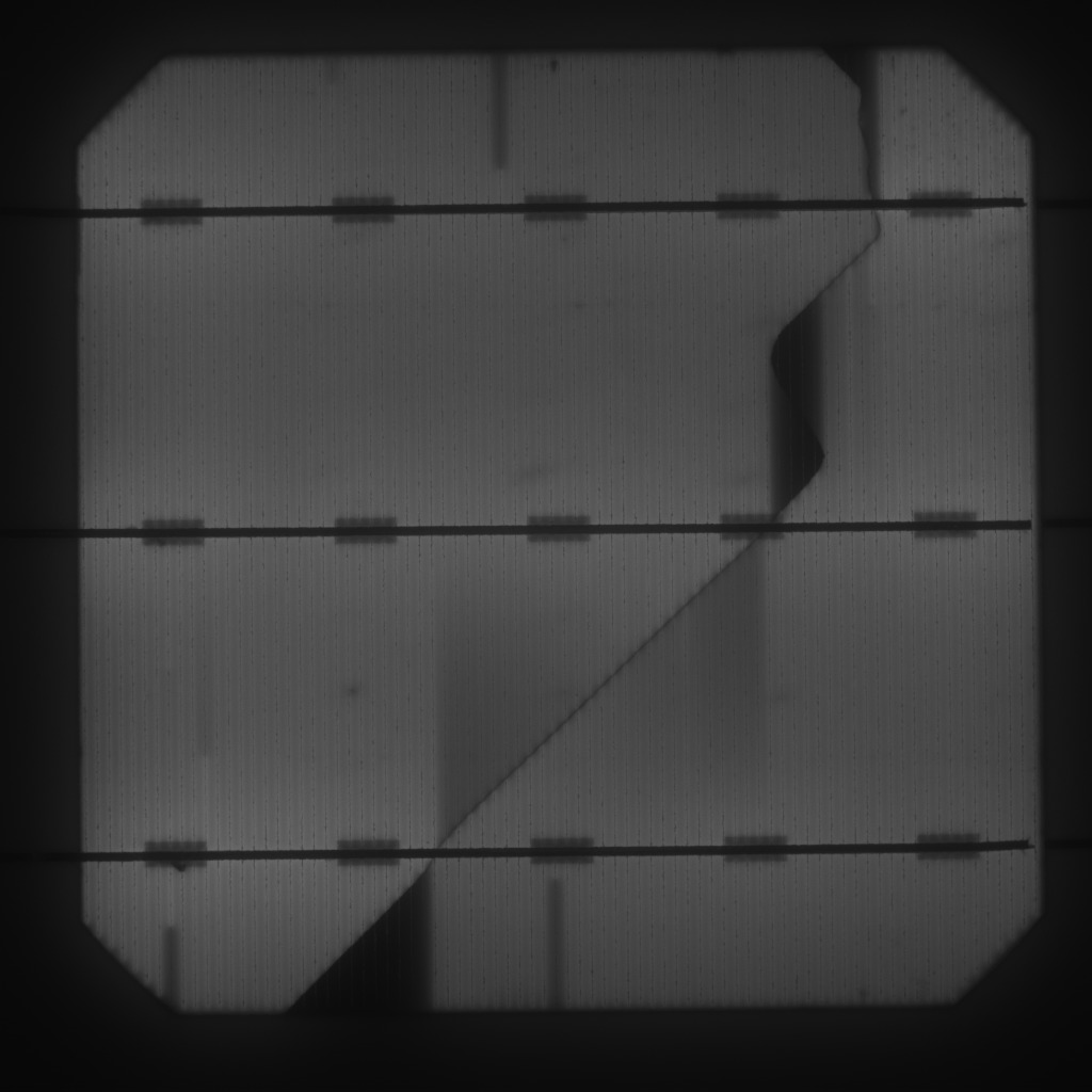
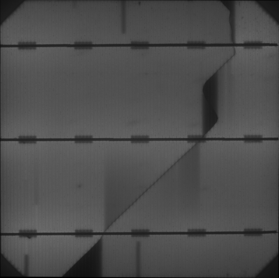
Figure 7: EL image of a mini-module (left) and the extracted and rescaled cell area using the one-cell extraction method.

7.2 Database simulation

To assess the performance of the proposed methods we employ the following scheme. First, all images of the database were corrected using the proposed preprocessing work-flow. The resulting corrected database was taken as ground truth. Next, a random sample of $100$ images was drawn. To each sampled image simulated random rotation, perspective and shift distortions were applied by drawing the characterizing parameters from probability distributions. The details of this parameterization and the choice of the distributions are given below. For every type of distortion (rotation, perspective, shift) $100$ different parameters resp. parameter vectors were drawn resulting in a total of $10^{4}$ images to which the preprocessing procedure was applied.

The accuracy of the method is measured by comparing the known (simulated) parameter vector, $\theta$, of distortion parameters with the estimated one, $\widehat{\theta}$, calculated from the preprocessing output image. As a measure we use the sum of absolute deviations (Manhattan distance),

$$SAD=\sum_{i}|\theta_{i}-\widehat{\theta}_{i}|,$$

separately calculated for rotation, perspective, module position and module size. In total, this simulation scheme provides $10^{4}$ values of each SAD, and these distributions were analyzed.

Before discussing the results, let us describe the details of the simulation step:

The rotation distortion is governed by a single parameter, the rotation angle, which is drawn from a uniform distribution on the interval $[-20,20]$ (measured in degrees).

The perspective distortion is governed by $8$ parameters, namely the coordinates of the distorted rectangle in Figure 1). We sample those $8$ parameters uniformly in a hyper-interval in such a way that the variation of the boundary lines of the rectangular PV module is approximately $\pm 5$ degrees.

Lastly, the shift was simulated with periodic boundary conditions, i.e. on a torus, in such a way that the PV module lies within the original image boundaries. This shift is parameterized by a two-dimensional vector: shifts along $x$ and $y$ axes. In addition, we considered the associated module size as a parameter.

It is worth mentioning that the ranges of the uniform distributions used here to simulate distortion effects lead to stronger distortions than present in our database of real EL images. These images were collected under outdoor conditions without demounting the PV modules, and therefore one can expect even higher accuracy when using the approach for image data collected under well-controlled conditions or in a lab.

After applying the simulated distortion effects, the preprocessing work-flow including the cell detection stage was run. Then the estimated parameter vector $\widehat{\theta}$ and its Manhattan distance to $\theta$ were determined. For the shift parameters the calculations are somewhat involved: For a PV module the distance between its top-left corner $x$ coordinate on the original module (before applying the random distortions) and its top-left corner $x$ coordinate on the output image (after applying preprocessing and cell detection) were calculated. Adding the corresponding distance of the $y$ coordinates gives the value of the SAD. At this point, it is worth recalling that the cell detection method was applied with accuracy parameter $R=5$.

The resulting distribution of the accuracy measured by SAD is depicted in Figure 8, where boxplots for the SAD of rotation, perspective, module position and module size are shown. The results demonstrate the high accuracy of the approach. For example, the measure for perspective distortion, the sum of the distances (in degree) of all four sides, is less than 1 degree except a few outliers and not larger than $0.6$ degree for $3/4$ of the cases.

Figure 8: Performance of the preprocessing methods for the database. Left to right: rotation distortion correction, perspective distortion correction and cell detection accuracy

We also remark that all preprocessing methods are applied with a fixed set of tuning parameters. The simulations not presented here indicate that there is almost no variation in performance for different EL images, and therefore, the selected set of tuning parameters adapt well for images in our database. However, there are few cases of images with relatively low visual contrast where a small difference in performance can be noticed. We address this issue in the next section.

7.3 Simulations for low and high contrast EL images

In order to investigate how the proposed approach performs depending on the image quality of an EL image, we selected two images from the database which are shown in Figure 9. On a high contrast image (right image in Figure 9) the grid lines are much better reproduced than on a low contrast image (left image). The selected low contrast image also suffers from severe vignetting, i.e. darkening of the corners, and it is somewhat underexposed. The inhomogeneity of the cell area, due to the multicrystalline silicon of that module, is also more pronounced than for the high contrast image. The question arises to which extent this has an effect on the accuracy of our method.

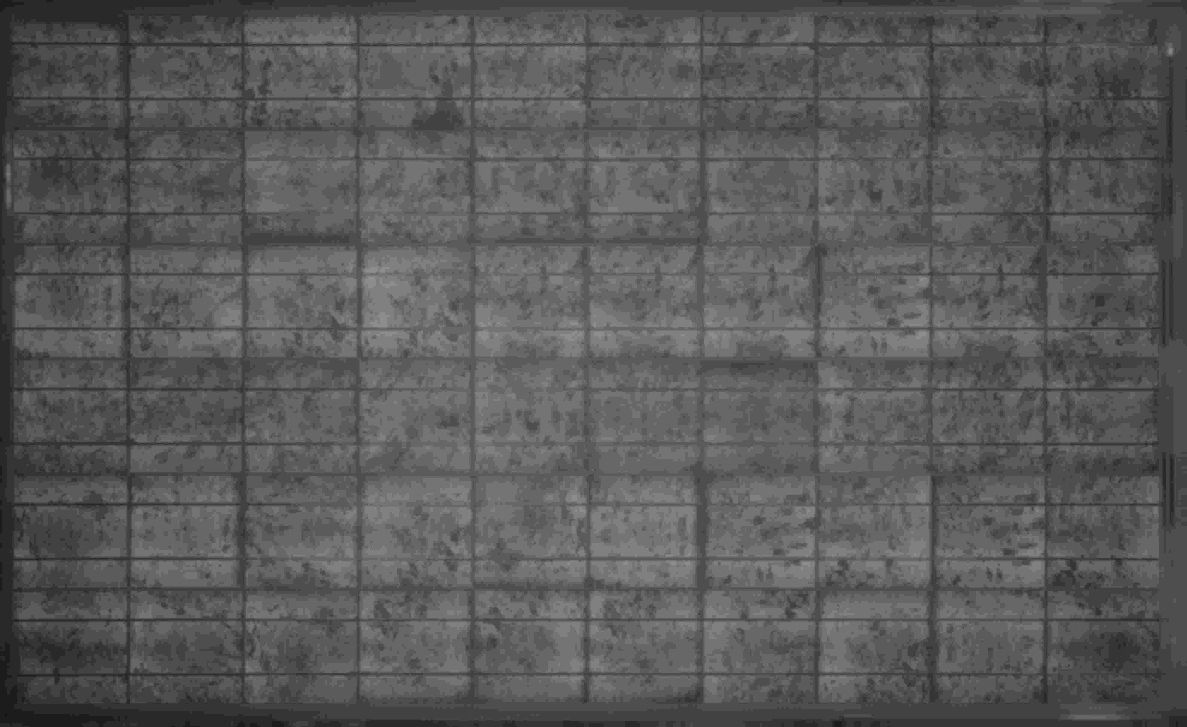
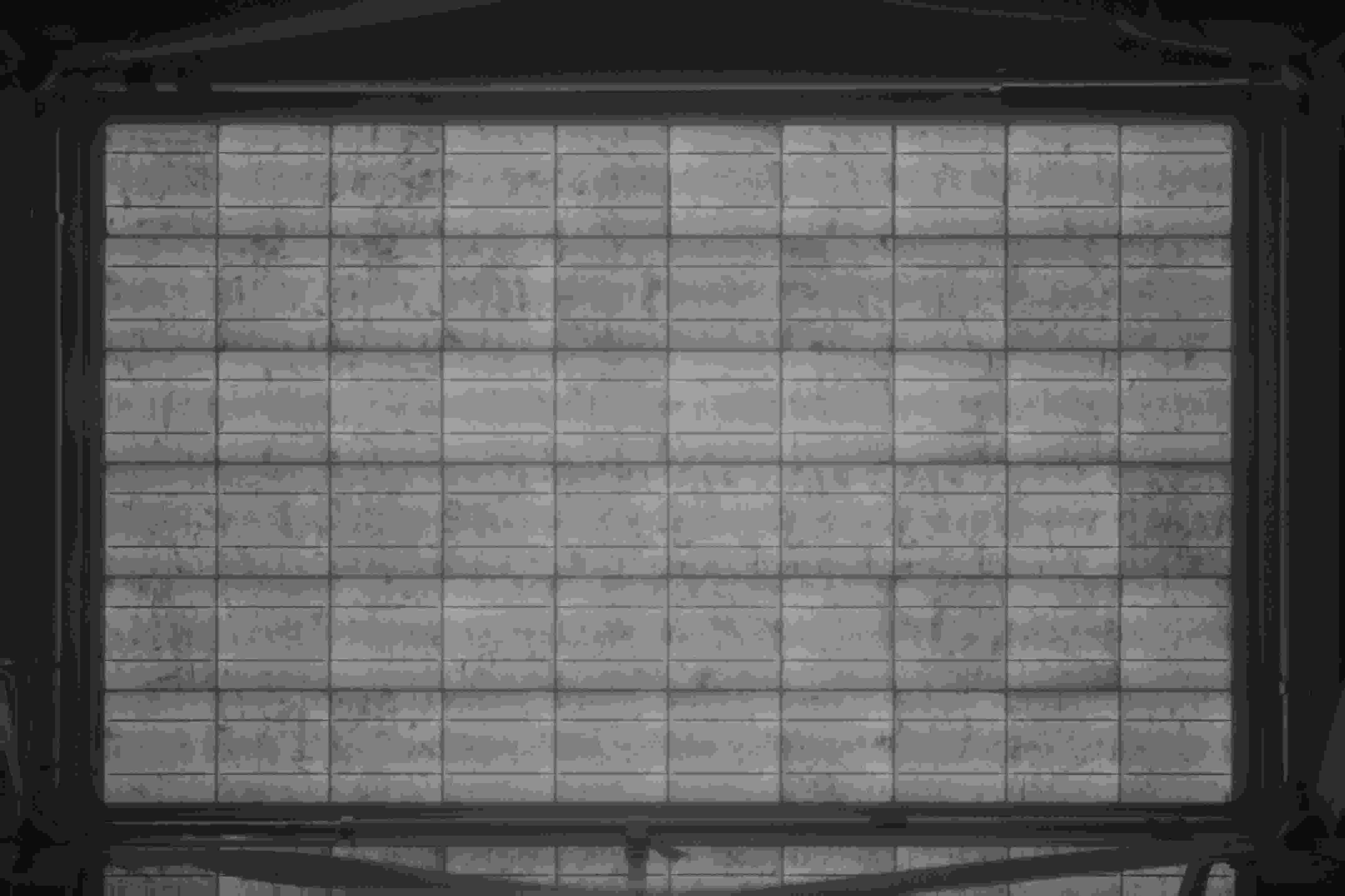
Figure 9: An example of two images with low (left image) and high (right image) contrast

The simulation scheme discussed above in detail was run for both images providing two distributions of sum of absolute differences (SAD) measure for each of the effects (rotation, perspective, module position, module size). The result is shown in Figure 10. It can be seen that image quality in terms of low contrast has an impact, but the accuracy is still very good. We may conclude that the proposed preprocessing framework is capable of dealing with low image contrast EL images. As a consequence, when mainstreaming the approach in an industrial production, one can expect reliable, robust and accurate performance even under high-throughput conditions.

Figure 10: Comparison of the performance for selected images with visually high and low contrast, respectively. Left to right: rotation distortion correction, perspective distortion correction and cell detection accuracy

8 Conclusions

Motivated by the problem to preprocess and analyze electroluminescence images of photovoltaic modules and detect all solar cells, this paper proposes a comprehensive methodology for preprocessing image data by correcting for distortions due to rotation, perspective, location and size. Further, two methods are proposed to detect and extract cells from an image, and the automatized algorithm outputs an image where the extracted and standardized cells are put together. The methods are optimized and to some extent tailor-made for photovoltaic images. But they can be certainly adapted to similar industrial imaging applications where the same problems arise. For example images of wafers consisting of electrical circuits such as CPUs, which are also arranged at fixed distances.

The approach combines specialized Hough transform algorithms, statistical tools such as robust regression and change-point estimation, as well as a priori knowledge from technical specifications, in order to provide a reliable and automatized work-flow to process such image data with high accuracy.

Extensive simulations were conducted to assess the accuracy of the methods for a database of real images from photovoltaics. One may conclude from the numerical results of these simulations that the overall procedure is accurate and reliably works even for massive image data sets. There are only a few cases where the distortions and/or the module position and size can not be recovered accurately. From a second simulation study, conducted for selected low and high contrast images, we can conclude that the approach is capable of dealing with low image quality as well. As a consequence, the approach reliably works for outdoor images and, when mainstreaming the proposal in industrial production, one can expect that it works well and reliable even under high-throughput conditions where ideal imaging conditions are difficult to guarantee.

Future work could study the adaption to other solar cell technologies, especially thin-film solar cells, take into account imaging schemes where each EL image consists of several pictures, as well as extend and adopt the approach to similar industrial imaging problems.

The authors would like to express their sincere appreciation for a grant from the German Ministry for Economic Affairs and Energie (BMWi), collaborative project PV-Scan, grant no. 0325588B. They thank Sunnyside upP, Cologne, International Solar Energy Research Center (ISC) Konstanz and TÜV Rheinland Energie GmbH, Cologne, for providing the EL image data and discussing results.

The comments and suggestions of anonymous reviewers are appreciated.

Appendix A Appendix

Denote $d_{l}\coloneqq\sqrt{(1-\delta_{l})^{2}+\delta_{l}^{2}}$, then conditions for the indicator function in (4) being non-zero are given by

$$B_{R}((a,b))\cap\mathcal{P}(x,y)\neq\emptyset\Leftrightarrow\exists l=0,\ldots,(n-1):$$

$$\left|a(1-\delta_{l})+b\delta_{l}-x\right|\leq Rd_{l},$$

subject to conditions

$$0\leq a,b\leq W,L\leq b-a\leq U.$$

$$\left\{\begin{array}[]{lll}b&\leq&\min\left(\frac{1+Rd_{l}}{\delta_{l}},W\right)\\ b&\geq&\max\left(\frac{1-W(1-\delta_{l})-Rd_{l}}{\delta_{l}},L\right)\\ a&\leq&\min\left(\frac{1-b\delta_{l}+Rd_{l}}{1-\delta_{l}},W,b-L\right)\\ a&\geq&\max\left(\frac{1-b\delta_{l}-Rd_{l}}{1-\delta_{l}},0,b-U\right)\end{array}\right..$$

References

- [1] G. Fischer, U. Hupach, J. Schmauder, A. Sepanski, A. Sommer, A. Steland and W. Vaasen, Failure assessments of PV systems demonstrate the importance of elective quality assurance, PV-Tech Power 14 (2018), 70–81.
- [2] A. Pepelyshev, E. Sovetkin and A. Steland, Panel-based stratified cluster sampling and analysis for photovoltaic outdoor measurements, Applied Stochastic Models in Business and Industry 33(1) (2017), 35–53.
- [3] T. Potthoff, K. Bothe, U. Eitner, D. Hinken and M. Köntges, Detection of the voltage distribution in photovoltaic modules by electromluminescence imaging, Progress in Photovoltaics 18 (2010), 100–106.
- [4] W. Herrmann, J. Althaus, A. Steland and H. Zähle, Statistical and experimental methods for assessing the power output specification of PV modules., Proceedings of the 21st European Photovoltaic Solar Energy Conference (2006), 2416–2420.
- [5] W. Herrmann and A. Steland, Evaluation of photovoltaic modules based on sampling inspection using smoothed empirical quantiles., Progress in Photovoltaics 18(1) (2010), 1–9.
- [6] A. Steland and H. Zähle, Sampling inspection by variables: Nonparametric setting., Statist. Neerlandica 63(1) (2009), 101–123.
- [7] A. Avellan-Hampe, A. Pepelyshev and A. Steland, Acceptance sampling plans for photovoltaic modules with two-sided specification limits., Progress in Photovoltaics (2013), in press.
- [8] A. Steland, Sampling plans for control-inspection schemes under independent and dependent sampling designs with applications to photovoltaics, Frontiers in Statistical Quality Control 11 (2015), 287–317, S. Knoth and W. Schmid.
- [9] D. Tsai, C. Chang and S. Chao, Macro-crack inspection in heterogeneously textured solar wafers using anisotropic diffusion, Image and Vision Computing 28 (2010), 491–501.
- [10] T. Sun, C. Tseng and M. Chen, Electric contacts inspection using machine vision, Image and Vision Computing 28 (2010), 890–901.
- [11] M.G. Mauk, Image processing for solar cell analysis, diagnostics and quality assurance inspection, Handbook of Research on Solar Energy Systems and Technologies Ch. 14(4) (2012), 338–375.
- [12] T. Fuyuki, H. Kondo, T. Yamazaki, Y. Takahashi and Y. Uraoka, Photographic surveying of minority carrier diffusion length in polycrystalline silicon solar cells by electroluminescence, Applied Physics Letters 86(26) (2005), 262108. doi:10.1063/1.1978979. https://doi.org/10.1063/1.1978979.
- [13] R. Evans, A. Sugianto and W. Mao, Interpreting module EL images for quality control, Proceedings of the 52nd Annual Conference of the Australian Solar Society (Australian Solar Council) (2014).
- [14] E.R. Davies, Machine Vision: Theory, Algorithms, Practicalities, 3rd edn, Morgan Kaufman, 2004.
- [15] I. Goodfellow, Y. Bengio and A. Courville, Deep Learning (Adaptive Computation and Machine Learning, MIT Press, 2016.
- [16] U. Shaham, A. Cloninger and R.R. Coifman, Provable approximation properties for deep neural networks, Appl. Comput. Harmon. Anal. 44(3) (2018), 537–557, ISSN 1063-5203. doi:10.1016/j.acha.2016.04.003. https://doi.org/10.1016/j.acha.2016.04.003.
- [17] A. Steland, Convergence of moments for approximating processes and applications to surrogate models like deep learning neural networks, International Journal of Statistics: Advances in Theory and Applications 2(1) (2018), 77–94.
- [18] M. Koziarski and B. Cyganek, Image recognition with deep neural networks in presence of noise - Dealing with and taking advantage of distortions, Integrated Computer-Aided Engineering 24(4) (2017), 337–349.
- [19] J. Fan, Detection of quadrilateral document regions from digital photographs, in: 2016 IEEE Winter Conference on Applications of Computer Vision (WACV), 2016, pp. 1–9. doi:10.1109/WACV.2016.7477661.
- [20] E.R. Davies, A generalised approach to the use of sampling for rapid object location, Int. J. Appl. Math. Comput. Sci. 18(1) (2008), 7–19, ISSN 1641-876X. doi:10.2478/v10006-008-0001-3. https://doi.org/10.2478/v10006-008-0001-3.
- [21] R. Hartley and S.B. Kang, Parameter-free radial distortion correction with center of distortion estimation, IEEE Transactions on Pattern Analysis and Machine Intelligence 29(8) (2007), 1309–1321.
- [22] D.M. Hawkins, Testing a sequence of observations for a shift in location, Journal of the American Statistical Association 72(357) (1977), 180–186.
- [23] J. Illingworth and J. Kittler, A survey of the Hough transform, Computer vision, graphics, and image processing 44(1) (1988), 87–116.
- [24] A. Goldenshluger and A. Zeevi, The Hough Transform Estimator., The Annals of Statistics 32(5) (2004), 1908–1932.
- [25] J. Matas, C. Galambos and J. Kittler, Robust detection of lines using the progressive probabilistic hough transform, Computer Vision and Image Understanding 78(1) (2000), 119–137.
- [26] D.H. Ballard, Generalizing the Hough transform to detect arbitrary shapes, Pattern recognition 13(2) (1981), 111–122.
- [27] J. Kiefer, Sequential minimax search for a maximum, Proceedings of the American Mathematical Society 4(3) (1953), 502–506.
- [28] J.F. Frazier, C.C. Reinhart and J.F. Alves, Automated license plate locator and reader including perspective distortion correction, Google Patents, 1997, US Patent 5,651,075.
- [29] T. Tan, G.D. Sullivan and K.D. Baker, On Computing The Perspective Transformation Matrix and Camera Parameters., in: BMVC, 1993, pp. 1–10.
- [30] E. Rafajłowicz, Susan Edge Detector Reinterpreted, Simplified and Modified., Proceedings of the 2007 International Workshop On Multidimensional (ND) Systems (2007).
- [31] E. Rafajłowicz, M. Pawlak and A. Steland, Nonlinear image processing and filtering: a unified approach based on vertically weighted regression, Int. J. Appl. Math. Comput. Sci. 18(1) (2008), 49–61.
- [32] A. Steland, Vertically weighted averages in Hilbert spaces and applications to imaging: fixed-sample asymptotics and efficient sequential two-stage estimation, Sequential Anal. 34(3) (2015), 295–323.
- [33] E. Sovetkin and A. Steland, On statistical preprocessing of PV field image data using robust regression, in: Advances in Mathematics and Statistical Sciences, WSEAS Press, 2015, pp. 48–51.
- [34] Image processing library, 2015, http://www.imagemagick.org/.
- [35] G. Bradski, OpenCV library, Dr. Dobb’s Journal of Software Tools (2000).