Applications of a class of Herglotz operator pencils.

Abstract

We identify a class of operator pencils, arising in a number of applications, which have only real eigenvalues. In the one-dimensional case we prove a novel version of the Sturm oscillation theorem: if the dependence on the eigenvalue parameter is of degree $k$ then the real axis can be partitioned into a union of $k$ disjoint intervals, each of which enjoys a Sturm oscillation theorem: on each interval there is an increasing sequence of eigenvalues that are indexed by the number of roots of the associated eigenfunction. One consequence of this is that it guarantees that the spectrum of these operator pencils has finite accumulation points, implying that the operators do not have compact resolvents. As an application we apply this theory to an epidemic model and several species dispersal models arising in biology.

1 Introduction

There are a number of contexts in which eigenvalue pencils arise in applied mathematics [9]. When studying the stability of standing waves and other coherent structures it is frequently the case that one must consider a non-self-adjoint eigenvalue pencil. In the context of integrable systems the scattering problem that diagonalizes an integrable nonlinear flow frequently takes the form of a eigenvalue pencil; take, for instance the Sine-Gordon equation in the laboratory frame [16] or the derivative nonlinear Schrödinger equation [8]. Additionally we will present a number of other problems arising in the analysis of biological problems where rational operator pencils arise. The difficulty with these problems, from the point of view of both analysis and numerical experimentation, is that one has no apriori information as to where the spectrum of the problem might lie. The purpose of this note is to point out a class of pencils, arising in a number of applications, which only admit real eigenvalues, namely those that depend on the spectral parameter in a Herglotz way. We show that a number of the properties of self-adjoint eigenvalue problems carry over to Herglotz operator pencils: the eigenvalues are real and semi-simple, and for second order rational Herglotz pencils we have an interesting generalization of the Sturm oscillation theorem. We begin by reminding the reader of the definition of a Herglotz function [15]. These functions are also sometimes referred to as Nevanlinna or Pick functions, but in the spectral theory literature they are most often referred to as Herglotz functions, so that is the usage that we will adopt here.

Definition 1.1.

A meromorphic function $f(\lambda)$ is Herglotz if $\operatorname{Im}(\lambda)>0$ (resp. $\operatorname{Im}(\lambda)<0$) implies that $\operatorname{Im}(f(\lambda))>0$ (resp. $\operatorname{Im}(f(\lambda))<0$))

The following is standard:

Proposition 1.2.

If $f(\lambda)$ is Herglotz then

• The zeroes and poles of $f(\lambda)$ lie on the real axis.

• If $\lambda$ is real and not a pole then $f^{\prime}(\lambda)>0$.

• The zeroes and poles of $f(\lambda)$ alternate on the real axis.

For the purposes of this paper the canonical example of a Herglotz function is the rational function

$$f(\lambda)=\sum_{i=1}^{N}\frac{A_{i}}{\alpha_{i}-\lambda}+B+C\lambda$$

with $A_{i},B,C$ real and positive and $\alpha_{i}$ real, as all of the problems we consider lead to rational operator pencils. More generally one has a representation formula for any Herglotz function

$$f(\lambda)=B+C\lambda+\int_{\mathbb{R}}\left(\frac{1}{x-\lambda}-\frac{\lambda}{1+\lambda^{2}}\right)d\mu(x)$$

for some measure $d\mu(x)$ but we are unaware of any applications that require this general representation.

2 Motivating Examples

In this section we present some examples intended to motivate the later discussion. As a first example we consider a reaction-diffusion equation of the form

(1) $$u_{t}=u_{xx}+f(u,v)$$

(2) $$v_{t}=g(u,v)$$

together with appropriate boundary conditions. Assuming that we can find a steady state solution

(3) $$u(x,t)=\bar{u}(x)$$

(4) $$v(x,t)=\bar{v}(x)$$

we consider the linearization of the evolution around the steady state $(\bar{u},\bar{v})$. This leads to the following equation for the tangent flow

(5) $$p_{t}=p_{xx}+\frac{\partial f}{\partial u}(\bar{u},\bar{v})p+\frac{\partial f}{\partial v}(\bar{u},\bar{v})q$$

(6) $$q_{t}=\frac{\partial g}{\partial u}(\bar{u},\bar{v})p+\frac{\partial g}{\partial v}(\bar{u},\bar{v})q$$

or, equivalently the linearized stability problem

(7) $$\lambda p=p_{xx}+\frac{\partial f}{\partial u}(\bar{u},\bar{v})p+\frac{\partial f}{\partial v}(\bar{u},\bar{v})q$$

(8) $$\lambda q=\frac{\partial g}{\partial u}(\bar{u},\bar{v})p+\frac{\partial g}{\partial v}(\bar{u},\bar{v})q$$

This is an ordinary, though non-selfadjoint eigenvalue problem, but after one eliminates the function $q$ it becomes a rational eigenvalue pencil.

$$\lambda p=p_{xx}+\frac{\partial f}{\partial u}(\bar{u},\bar{v})p+\frac{\partial f}{\partial v}(\bar{u},\bar{v})\frac{\partial g}{\partial u}(\bar{u},\bar{v})\frac{1}{\lambda-\frac{\partial g}{\partial v}(\bar{u},\bar{v})}$$

The main observation is that under the sign condition $f_{v}g_{u}(\bar{u},\bar{v})\geq 0$ the right hand side of the operator pencil is (for $x$ fixed), a Herglotz function which implies some very nice behavior in the eigenvalue problem, including (as we shall see) reality of the spectrum and semi-simplicity of the eigenvalues. This generalizes the case when $f_{v}=g_{u}$, for which case the flow is a gradient and the second variation is obviously self-adjoint.

One could object that the original system (7, 8) is, in fact, self-adjoint under the modified inner product $\|(p,q)\|_{2}^{2}=\int v^{2}+\frac{f_{w}}{g_{v}}w^{2}$ when the sign condition $f_{w}g_{v}>0$ is met. In some sense this must happen, since it is an old theorem of Drazin and Haynsworth [3] that any matrix having all real eigenvalues and $n$ linearly independent eigenvectors is self-adjoint under some appropriate inner product. However, in general it is unclear how to check whether there exists an inner product rendering a given operator self-adjoint. Checking that a given function is Herglotz, on the other hand, is relatively straightforward, and amounts (for a rational pencil) to checking a finite number of reality/sign conditions.

One biological model that falls into this class is the following system modeling the spread of a human disease through infective propagules [2]

(9) $$u_{t} = du_{xx}-a_{11}u+a_{12}v=du_{xx}+f(u,v)$$

(10) $$v_{t} = \tilde{g}(u)-a_{22}v=g(u,v).$$

Here, $u$ denotes the spatial density of the infectious propagules, $v$ denotes the density of the human infective class; the parameters $d,a_{ij}>0$; the function $\tilde{g}:\mathbb{R}_{+}\to\mathbb{R}_{+}$ and $\tilde{g}^{\prime}(u)>0$ for $u>0$. Then, the corresponding eigenvalue problem reads

$$dp_{xx}-a_{11}p=\lambda p-a_{12}\tilde{g}^{\prime}\frac{1}{\lambda+a_{22}}p.$$

Since $a_{12}\tilde{g}^{\prime}>0$ the condition for the reality of the spectrum follows.

Equations of similar form also arise in combustion, typically solid combustion. In this situation heat is free to diffuse but the solid reactant does not diffuse, at least on combustion time-scales. For work on this problem we refer the reader to the article of Ghazaryan, Latushkin and Schechter [5, 6], but we do note that in such combustion problems the sign condition is typically not met: in the combustion context one expects $f_{w}g_{u}<0.$

Similarly we can consider a system with three reacting species, one of which is allowed to diffuse

$$u_{t}=u_{xx}+f(u,v,w)$$

(11) $$v_{t}=g(u,v,w)$$

$$w_{t}=h(u,v,w).$$

Linearizing about a steady state solution yields the following eigenvalue problem

$$\lambda p=p_{xx}+f_{u}p+f_{v}q+f_{w}s$$

$$\lambda q=g_{u}p+g_{v}q+g_{w}s$$

$$\lambda s=h_{u}p+h_{v}q+h_{w}s$$

Solving the last two for $q,s$ in terms of $p$ results in

$$q=\frac{g_{u}(\lambda-h_{w})+h_{u}g_{w}}{(\lambda-g_{v})(\lambda-h_{w})-g_{w}h_{v}}p,~{}~{}s=\frac{(\lambda-g_{v})h_{u}+h_{v}g_{u}}{(\lambda-g_{v})(\lambda-h_{w})-g_{w}h_{v}}p$$

and substituting into the first equation yields

$$p_{xx}+f_{u}p=\left(\lambda-f_{v}\frac{g_{u}(\lambda-h_{w})+h_{u}g_{w}}{(\lambda-g_{v})(\lambda-h_{w})-g_{w}h_{v}}-f_{w}\frac{h_{u}(\lambda-g_{v})+h_{v}g_{u}}{(\lambda-g_{v})(\lambda-h_{w})-g_{w}h_{v}}\right)p\equiv H(\lambda)p$$

$$p_{xx}+f_{u}p=\left(\lambda-\frac{\alpha(x)\lambda+\beta(x)}{\lambda^{2}+\gamma(x)\lambda+\delta(x)}\right)$$

The function $\lambda-\frac{\alpha(x)\lambda+\beta(x)}{\lambda^{2}+\gamma(x)\lambda+\delta}$ is (for fixed $x$) a Herglotz function of $\lambda$ if and only if the following conditions are met

• The roots of $\lambda^{2}+\gamma(x)\lambda+\delta(x)$ are real.

• The residues of the function $\frac{\alpha(x)\lambda+\beta(x)}{\lambda^{2}+\gamma(x)\lambda+\delta}$ at the roots are positive.

The above two conditions translate into the following sign conditions on the coefficients.

• $\beta\gamma-\alpha\delta>0$

• $\beta^{2}-\alpha(\beta\gamma-\alpha\delta)<0$

Equivalently, reality of the spectrum follows if

(20) $$\left|\begin{array}[]{cc}f_{v}&f_{w}\\ g_{v}&g_{w}\end{array}\right|\left|\begin{array}[]{cc}g_{u}&g_{v}\\ h_{u}&h_{v}\end{array}\right|+\left|\begin{array}[]{cc}f_{v}&f_{w}\\ h_{v}&h_{w}\end{array}\right|\left|\begin{array}[]{cc}g_{u}&g_{w}\\ h_{u}&h_{w}\end{array}\right|>0~{}~{}\mbox{and}$$

(29) $$\left(h_{u}\left|\begin{array}[]{cc}g_{u}&g_{w}\\ h_{u}&h_{w}\end{array}\right|+g_{u}\left|\begin{array}[]{cc}g_{u}&g_{v}\\ h_{u}&h_{v}\end{array}\right|\right)\left(f_{v}\left|\begin{array}[]{cc}f_{v}&f_{w}\\ g_{v}&g_{w}\end{array}\right|+f_{w}\left|\begin{array}[]{cc}f_{v}&f_{w}\\ h_{v}&h_{w}\end{array}\right|\right)>0$$

A system in the form of (11) is considered in [4] as a model of the dynamics of two plants $v,w$ and one herbivore $u$

$$u_{t} = du_{xx}+\left(b_{1}s_{1}v+b_{2}s_{2}w\left(1-\frac{s_{2}w}{4n(1+h_{1}s_{1}v+h_{2}s_{2}w)}\right)-m\right)\frac{u}{1+h_{1}s_{1}v+h_{2}s_{2}w}$$

$$= du_{xx}+f(u,v,w)$$

$$v_{t} = r_{1}v\left(1-(v+a_{12}w)\right)-\frac{s_{1}uv}{1+h_{1}s_{1}v+h_{2}s_{2}w}=g(u,v,w),$$

$$w_{t} = r_{2}w\left(1-(w+a_{21}v)\right)-\frac{s_{2}uw}{1+h_{1}s_{1}v+h_{2}s_{2}w}\left(1-\frac{s_{2}w}{4n(1+h_{1}s_{1}v+h_{2}s_{2}w)}\right)=h(u,v,w),$$

where $d,a_{ij}>0$ and all other parameters are positive.

In [11] three models of morphogen concentrations were analyzed. Nonlinear reaction-diffusion equations were used to model morphogen gradients that arise in the patterning of Drosophila wings. In a series of works, the authors showed that the linear stability analysis of steady state solutions yields a nonlinear eigenvalue problem. They also demonstrated that the spectrum is real and stable. In this section, we will offer an alternative proof of these facts using our main result.

Following the notation in [11], the dimensionless normalized concentration of the diffusing morphogen species is denoted with $a(x,t)$ and that of the morphogens that are bound to receptors is denoted by $b(x,t)$. Then, the system reads

$$\frac{\partial a}{\partial t}=\frac{\partial^{2}a}{\partial x^{2}}-h_{0}a(1-b)+f_{0}b,~{}~{}x\in(0,1),~{}~{}t>0,~{}~{}$$

(30) $$\frac{\partial a(0,t)}{\partial t}=\nu_{0}-h_{o}a(0,t)(1-b(0,t))+f_{0}b(0,t),~{}~{}a(1,t)=0$$

(31) $$\frac{\partial b}{\partial t}=h_{0}a(1-b)-(f_{0}+g_{0})b,~{}~{}x\in[0,1],~{}~{}t>0.$$

Here, the constants $h_{0},f_{0},g_{0},\nu_{0}$ are positive and correspond to normalized rates.

If one linearizes about the time-independent steady-state solution $\left(\bar{a}(x),~{}\bar{b}(x)\right)$ considering solutions of the form

$$a(x,t)=\bar{a}(x)+e^{\lambda t}\hat{a}(x),~{}~{}b(x,t)=\bar{b}(x)+e^{\lambda t}\hat{b}(x,t),$$

and after some standard algebra to eliminate the algebraic equation for the bound morphogen $b$, the following nonlinear eigenvalue problem is obtained

(32) $$\hat{a}_{xx}-\left(\lambda+q(x,\lambda)\right)\hat{a}=0,~{}~{}\mbox{where}~{}~{}q(x,\lambda)=\frac{h_{0}(f_{0}+g_{0})}{f_{0}+g_{0}+h_{0}\bar{a}}\frac{\lambda+g_{0}}{\lambda+f_{0}+g_{0}+h_{0}\bar{a}},$$

together with appropriate boundary conditions.

One easily notices that $q(x,\lambda)$ is a Herglotz function, since

$$f_{0}+g_{0}+h_{0}\bar{a}-g_{0}=f_{0}+h_{0}\bar{a}>0.$$

Therefore,

$$Q(x,\lambda)=\lambda+q(x,\lambda)$$

is a Herglotz function as well. Using our main result it then follows that the spectrum is real.

As these examples illustrate, a wealth of biological models have similar structure. Their common theme is that some degrees of freedom permit diffusion or mobility, while others do not. In many compartmental systems arising in biological applications, some of the components are mobile (such as herbivores and pollinators) while others are not (such as plants) [4, 10, 12, 14]. In epidemic compartmental models, such distinctions between mobile and motionless compartments also arise [2, 13, 18] due to the fact that infected animals are mainly responsible for spreading the disease, or when infective propagules disperse randomly while the infected population is characterized by small mobility. Another setting where such models arise is in pattern formation, where diffusing morphogens interact with others that are bound to cell receptors [11].

The final example is more theoretical, and is motivated by work of Kapitula and Promislow [7] on the so-called Krein matrix method. Consider a self-adjoint eigenvalue problem that can be written in the following block-partitioned form

$$({\bf H}-\lambda)v=\left(\begin{array}[]{cc}{\bf A}-\lambda&{\bf B}\\ {\bf B}^{t}&{\bf C}-\lambda\end{array}\right)v=0,$$

with ${\bf A}={\bf A}^{t}$ and ${\bf C}={\bf C}^{t}$. The main idea is that, if we algebraically eliminate certain degrees of freedom, we are naturally led to a Herglotz pencil. To see this note that, if $\lambda$ is in the resolvent set of ${\bf C}$ then we have the following identity.

$${\bf U}{\bf H}{\bf U}^{t} =\left(\begin{array}[]{cc}{\bf I}&-{\bf B}({\bf C}-\lambda)^{-1}\\ 0&{\bf I}\end{array}\right)\left(\begin{array}[]{cc}{\bf A}&{\bf B}\\ {\bf B}^{t}&{\bf C}\end{array}\right)\left(\begin{array}[]{cc}{\bf I}&0\\ -({\bf C}-\lambda)^{-1}{\bf B}^{t}&{\bf I}\end{array}\right)$$

$$=\left(\begin{array}[]{cc}{\bf A}-\lambda-{\bf B}^{t}({\bf C}-\lambda)^{-1}{\bf B}&0\\ 0&({\bf C}-\lambda)\end{array}\right)$$

Therefore for $\lambda$ in the resolvent set of ${\bf C}$ the operator ${\bf U}$ is bounded and invertible and the eigenvalues of the full operator are eigenvalues of the Herglotz operator pencil ${\bf A}-\lambda-{\bf B}^{t}({\bf C}-\lambda)^{-1}{\bf B}.$ If $\lambda$ is in the spectrum of ${\bf C}$ (the complement of the resolvent set) one must do additional work to determine whether or not $\lambda$ is an eigenvalue of the full problem – see the work of Kapitula and Promislow for details. This example shows that Schur reduction of a self-adjoint eigenvalue problem leads naturally to a Herglotz operator pencil, and further motivates the idea that Herglotz pencils should behave like self-adjoint eigenvalue problems.

3 Main Results

Our basic observation is that the standard elementary argument that the spectrum of a self-adjoint operator is real carries over in a natural way to operator pencils that depend on the eigenvalue in a Herglotz way. The main claim of this paper is

Theorem 3.1.

Suppose that we have an eigenvalue pencil of the form

$${\bf H}\psi=\left(A_{0}\lambda-\sum_{k=1}\frac{A_{i}}{\lambda-\alpha_{i}}\right)\psi$$

where ${\bf H}$ is a self-adjoint operator on some domain $\operatorname{dom}({\bf H})$, and ${\bf A}_{i}$ are self-adjoint positive definite operators on $\operatorname{dom}({\bf H})$. Then the eigenvalue pencil has only real eigenvalues. Furthermore the eigenvalues are semi-simple.

Proof.

Suppose that $\lambda$ is an eigenvalue with eigenfunction $\psi$. Taking the inner product of both sides with $\psi$ we have that

$$\langle\psi,{\bf H}\psi\rangle=\langle\psi,{\bf A}_{0}\psi\rangle\lambda-\sum_{k=1}\frac{\langle\psi,{\bf A}_{k}\psi\rangle}{\lambda-\alpha_{i}}$$

From the self-adjointness of ${\bf H}$ we have that the left-hand side is purely real; the righthand side is a Herglotz function. Thus, if $\psi(x)$ is an eigenfunction the $\lambda$ is a root of some Hergoltz function $\tilde{g}_{\psi}(\lambda)$ and therefore must be real.

To see the semi-simplicity of the eigenvalues note that the condition for the existence of a Jordan chain for an operator pencil is the existence of a solution to

$${\bf M}(\lambda_{0})\psi_{0}=0$$

$${\bf M}(\lambda_{0})\psi_{1}+\frac{d{\bf M}}{d\lambda}(\lambda_{0})\psi_{0}=0$$

with $\psi_{0}$ non-zero. Taking the inner product of the second equation with $\psi_{0}$ gives

$$\langle\psi_{0},\frac{d{\bf M}}{d\lambda}(\lambda_{0})\psi_{0}\rangle=0,$$

but the Herglotz nature of the operator implies that the operator $\frac{d{\bf M}}{d\lambda}(\lambda_{0})$ is positive definite.

Next we specialize to the rational Sturm-Liouville problem

(33) $$-(D(x)p_{x})_{x}=\lambda W_{0}(x)p-\sum_{i=1}^{N}\frac{W_{i}(x)}{\lambda-\alpha_{i}}-V(x)p=g(x,\lambda)p;\quad p_{x}(0)=0=p_{x}(L)$$

As motivation for the next result we note that in the special case in which $V(x),W_{i}(x)$ and $D(x)$ are all constant we have that the solution is given by

$$p(x)=\cos\sqrt{\frac{g(\lambda)}{D}}x$$

with the eigenvalue condition $g(\lambda)=k^{2}\pi^{2}D$. Since $g(\lambda)$ is Herglotz it is monotone and takes every real value for $\lambda\in(\alpha_{i-1},\alpha_{i})$. Thus we have that for each such interval $(\alpha_{i-1},\alpha_{i})$ there is a sequence of eigenfunctions $p_{k}(x)$ which are indexed by $k$, the number of roots in $(\alpha_{i-1},\alpha_{i})$.

Equation (33) will typically not, of course, be solvable in closed form but in the WKB approximation, which is valid when $g(x,\lambda)$ is large (which occurs for $\lambda=\alpha_{I}^{-}$) we have the approximate eigenfunction

(34) $$p_{k}(x,\lambda)\approx\frac{\cos\left(\int_{0}^{x}\sqrt{\frac{g(x,\lambda)}{D(x)}}\right)}{\sqrt{D(x)}(g(x,\lambda))^{\frac{1}{4}}}$$

where the WKB quantization condition is that

(35) $$\int_{0}^{L}\sqrt{\frac{g(x,\lambda)}{D(x)}}dx=k\pi.$$

Since the quantity $\int_{0}^{L}\sqrt{\frac{g(x,\lambda)}{D(x)}}dx$ is a monotone function of $\lambda$ whenever $g(x,\lambda)$ is positive it follows that there is an increasing sequence of (approximate) eigenvalues asymptotic to $\alpha_{i}^{-}$ in each interval $(\alpha_{i-1},\alpha_{i})$.

These heuristics motivate the following version of the classical Sturm theorem.

Theorem 3.2.

Consider the rational Sturm Liouville pencil subject to Neumann boundary conditions

$$-(D(x)p_{x})_{x}=\lambda W_{0}(x)p-\sum_{i=1}^{N}\frac{W_{i}(x)}{\lambda-\alpha_{i}}-V(x)p=g(x,\lambda)p,\qquad p_{x}(a)=0=p_{x}(b)$$

with $D(x),V(x),W_{i}(x)$ continuous on $[a,b]$ and $D(x),W_{i}(x)>0$ on $[a,b]$. The quantities $\{\alpha_{i}\}_{i=1}^{N}$ will be referred to as the singular values. For ease of notation we will let $\alpha_{0}=-\infty$ and $\alpha_{N+1}=+\infty$, and will let $I_{j},~{}~{}~{}j\in 0\ldots N$ denote the interval $I_{j}=(\alpha_{j},\alpha_{j+1}).$ From the previous result the eigenvalues are real and semi-simple. Additionally the following oscillation results hold.

• Sturm Theorem For each integer $k\geq 0$ there exists one eigenvalue $\lambda_{k}^{j}$ in each interval $I_{j}=(\alpha_{j},\alpha_{j+1})~{}~{}~{}j\in 0\ldots N$ such that the corresponding eigenfunction $p_{k}^{j}(x)$ has exactly $k$ zeroes in the open interval $(a,b)$.

• By definition we have that $\lambda_{k}^{j}>\lambda_{k}^{j^{\prime}}$ if $j>j^{\prime}$. Further we have that $\lambda_{k}^{j}>\lambda_{k^{\prime}}^{j}$ if $k>k^{\prime}$.

• Each $\alpha_{i}$ except $\alpha_{0}$ is an accumulation point of eigenvalues, so $\alpha_{i},\,i\in 1\ldots N$ are in the essential spectrum.

In other words we have a Sturm oscillation type theorem that holds in every interval $(\alpha_{i},\alpha_{i+1})$: the eigenvalues in each such interval are increasing and indexed by the number of roots of the corresponding eigenfunction in $(a,b)$.

Remarks 3.3.

We first note that the fact that the pencil has finite accumulation points of eigenvalues means that the original operator is neither compact nor does it have compact resolvent. This illustrates that the problem in which some species do not diffuse is a singular perturbation of the problem in which those same species have a small diffusion coefficient, since in that case it is straightforward to see that the operator has compact resolvent.

We also note that the more general operator

$$-\frac{d}{dx}\left(D(x)u_{x}\right)=\lambda u-\sum_{i=1}^{N}\frac{W_{i}(x)}{\lambda-\alpha_{i}(x)}$$

has only real eigenvalues by the argument given previously but has essential spectrum for $\lambda\in\cup_{i=1}^{N}\operatorname{ran}(\alpha_{i}(x))$. This type of operator has been analyzed by Adamjan, Langer and Langer [1] for $N=1$, including construction of the spectral measure corresponding to the essential spectrum.

Proof.

The proof hinges on the fact that the (eigenvalue dependent) potential $g(x,\lambda)$ has the property that

• $g(x,\lambda)\rightarrow-\infty$ as $\lambda\rightarrow\alpha_{i}^{+}$

• $g(x,\lambda)\rightarrow+\infty$ as $\lambda\rightarrow\alpha_{i+1}^{-}.$

• $\frac{\partial g}{\partial\lambda}>0,$

which are essentially the conditions needed to apply the classical Sturm oscillation theorem for a one dimensional second order operator. For the convenience of the reader a proof is given in Appendix A.

Example 3.4.

To illustrate this theorem we consider the rational Sturm-Liouville pencil

$$-u_{xx}+\sin(x)u=\lambda u-\frac{.2+\cos^{2}(x)}{\lambda-2}u,\qquad u(0)=0=u(\pi)$$

which is equivalent to the system

$$-u_{xx}+\sin(x)u+v=\lambda u;\qquad u(0)=0=u(\pi)$$

(36) $$\alpha u+(.2+\cos^{2}(x))u=\lambda v$$

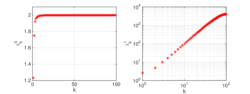
Figure 1: Eigenvalues for Eqn. (36)

There is one singular value, $\alpha_{1}=2$, and two open intervals on the real line for which ${\bf H}(\lambda)$ is defined, $(-\infty,2)$ and $(2,+\infty)$. We solved the system (36) numerically as described in Appendix B.

Using the discretization described with $n_{x}=100$ (see Appendix B for details), we will have 99 eigenvalues in the interval $I_{0}=(-\infty,2)$, denoted $\lambda^{0}_{k}$, and 99 eigenvalues in the interval $I_{1}=(2,\infty)$, denoted $\lambda^{1}_{k}$. The first set ($\lambda^{0}_{k}$) will have an accumulation point at $\alpha_{1}=2$, the second set ($\lambda^{1}_{k}$) at $\alpha_{2}=\infty$; this is shown in Fig. 1. The corresponding eigenfunctions we will index in the same way: i.e. as $u^{j}_{k}$ for the $k$th eigenvalue in interval $I_{j}$. We compare these eigenvalues with the WKB prediction $\frac{1}{\pi}\int_{0}^{\pi}\sqrt{\lambda-\sin(x)-\frac{.2+\cos^{2}(x)}{\lambda-2}}dx=k$, which we also evaluated numerically.

The numerical values of eigenvalues for $k\in 0\ldots 4$ are:

$\lambda$ Interval	$k=0$	$k=1$	$k=2$	$k=3$	$k=4$
$(-\infty,2)$ (Numerical)	1.22	1.75	1.92	1.95	1.97
$(-\infty,2)$ (WKB)	1.029	1.773	1.916	1.956	1.973
$(2,\infty)$ (Numerical)	2.59	4.88	9.65	16.53	25.41
$(2,\infty)$ (WKB)	2.68	4.88	9.73	16.69	25.67

The corresponding eigenfunctions, $u^{0}_{k}$ and $u^{1}_{k}$, are shown in Fig. 2. The left column shows the primary ($u^{0}_{k}$) and auxiliary eigenfunctions ($v^{0}_{k}$) for the interval $I_{0}$, while the right column shows $u^{1}_{k}$ and $v^{1}_{k}$. Note that $u^{j}_{k}$ has exactly $k$ zeros, as expected, and that the nodal sets of $u^{j}_{k}$ and $v^{j}_{k}$ coincide for each $j,k$. The functions $u^{0}_{k}$ and $v^{0}_{k}$ are of opposite sign, since $\lambda^{0}_{k}<2$, while $u^{1}_{k}$ and $v^{1}_{k}$ are same-signed.

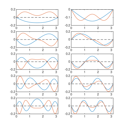
Figure 2: Left column: Eigenfunctions corresponding to $\lambda\in(-\infty,2)$. Both primary $u$ (blue) and auxiliary $v$ functions (red) are shown. From top to bottom: $u^{0}_{k}$ and $v^{0}_{k}$, for $k=0,1,2,3$ and $4$. Right column: same, but for $\lambda\in(2,\infty)$; i.e. $u^{1}_{k}$ and $v^{1}_{k}$

We next use Eqn. (34), (35) to make the following prediction for the asymptotics of the eigenvalues accumulating near $\lambda=2$:

$$\lambda_{k}^{0}\approx 2-\frac{\left(\frac{1}{\pi}\int_{0}^{\pi}\sqrt{.2+\cos^{2}(x)}\right)^{2}}{k^{2}}+O(k^{-3})\approx 2-\frac{.649}{k^{2}},$$

while the other branch of eigenvalues has the asymptotics

$$\lambda_{k}^{1}\approx k^{2}+O(1)$$

The plots in Figure 3 depicts a graph of $(\lambda_{k}^{1}-2)k^{2}$ vs $k$ for the eigenvalues in the region $(-\infty,2)$ together with a plot of $\lambda^{2}_{k}k^{-2}$ vs. $k$ for the eigenvalues in the region $(2,\infty)$. These are expected to asymptote to $.649$ and $1$ respectively. This is repeated for three different values of $\Delta x$, the discretization size, in order to assess the role of discretization error. In each case we see that the eigenvalue curve hugs the asymptote for a while before falling away due to discretization error, and that as the size of the discretization is decreased the curve hugs the presumed asymptotic value for longer, as one would expect.

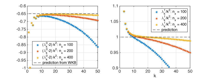
Figure 3: Asymptotics for the eigenvalues of Eqn. (36). Left: $(\lambda^{0}_{k}-2)k^{2}$, confirming a WKB calculation for eigenvalues that accumulate at $\alpha_{1}=2$. Right: $\lambda^{2}_{k}/k^{2}$ for eigenvalues that accumulate at $\alpha_{2}=\infty$, showing $k^{2}$ scaling.

4 Application: Spatial models in epidemiology

We now consider an example with detailed numerics.

Variable	Unit
$S$ susceptible host density	foxes/km2
$E$ exposed host density	foxes/km2
$I$ infected hosts density	foxes/km2
$t$ time	year
Parameter	Value
$a$ : average birth rate	1 per year
$b$ : average intrinsic death rate	0.5 per year
$1/\alpha(x)$ : average duration of clinical disease	$\approx 5$ days
$1/\sigma$ : average incubation period	28 days
$\beta(x)$ : disease transmission coefficient	$\approx 80$ km2 per year
$K$ : carrying capacity	0.25 to 4 foxes per km2
$D$ : diffusion coefficient	50 to 330 km2 per year

In [13] the following one-dimensional model for the spread of rabies among foxes was considered.

$$\frac{\partial E}{\partial t}=\beta(x)IS-\sigma E-\left(b+(a-b)\frac{N}{K}\right)E$$

$$\frac{\partial I}{\partial t}=\frac{\partial}{\partial x}\left(D(x)\frac{\partial I}{\partial x}\right)+\sigma E-\alpha(x)I-\left(b+(a-b)\frac{N}{K}\right)I$$

$$\frac{\partial S}{\partial t}=(a-b)\left(1-\frac{N}{K}\right)S-\beta(x)IS$$

$$\frac{\partial I}{\partial\eta}|_{\partial\Omega}=0,$$

where $S,E$ and $I$ are the population densities of the susceptible, exposed and infectious foxes, respectively and $N=S+E+I$ is the total fox population. When susceptible hosts contact infectious ones, they become exposed at rate $\beta(x)$. Exposed hosts remain in that class for an average period of $\sigma^{-1}$ before they transition into the infectious class. Hosts remain infectious for an average period of $\alpha(x)^{-1}$ before they die. While infectious, hosts experience random wandering; this movement is modeled as diffusion with coefficient $D(x)$. All host classes experience average birth rate $a$ and death rate $b$. They also compete for resources and so it is assumed that the environmental carrying capacity is $K$. Typical parameter values are given in the table above.

The authors [13] assumed that $\alpha,\beta,D$ are positive continuous functions depending on the spatial variable $x$. In this case there is the disease-free steady state $(E=0,I=0,S=K)$. Linearizing about the steady state gives the eigenvalue problem

$$-(\sigma+a)E+\beta(x)KI=\lambda E$$

(37) $$\frac{\partial}{\partial x}\left(D(x)\frac{\partial I}{\partial x}\right)+\sigma E-(\alpha(x)+a)I=\lambda I$$

$$\frac{\partial I}{\partial x}|_{\partial\Omega}=0.$$

Algebraically eliminating $E$ gives the eigenvalue pencil

$$\frac{\partial}{\partial x}\left(D(x)\frac{\partial I}{\partial x}\right)-(\alpha(x)+a)I=\left(\lambda-\frac{\sigma\beta(x)K}{\lambda+\sigma+a}\right)I=g(\lambda,x)I\qquad\frac{\partial I}{\partial x}|_{\partial\Omega}=0.$$

Our first observation is that the function $g(\lambda,x)=\lambda-\frac{\sigma\beta(x)K}{\lambda+\sigma+a}$ is a Herglotz function for all $x$ as long as $\sigma,\beta(x),K,a>0$, and thus the eigenvalues of this problem are all real.

This model was later considered by Wang and Zhao[18], who used the next-generation operator approach [17] to give a recipe for computing the reproduction number, $R_{0}$, and understanding its dependence on parameters in the spatially heterogeneous problem. The basic reproductive number $R_{0}$ is an important epidemiological threshold, since it determines whether the disease can invade the population (with $R_{0}>1$ indicating that the disease-free steady state is unstable) or not (with $R_{0}<1$ indicating that the disease-free steady state is locally asymptotically stable).

Defining $\tilde{\lambda}=-\lambda$, we see that the eigenvalue problem directly above can be written as:

(38) $$-\frac{d}{dx}\left(D(x)\frac{dI}{dx}\right)+(\alpha(x)+a)I+\frac{\sigma\beta(x)K}{\tilde{\lambda}-(\sigma+a)} = \tilde{\lambda}I;\;\frac{dI}{dx}|_{\partial\Omega}=0$$

to which we can immediately apply Theorem 3.2 to see that this has a smallest real eigenvalue which is simple and which will govern stability of Eqn. (37) (this is Lemma 4.1 from [18]).

Wang and Zhao analyze $R_{0}$ through a related eigenvalue problem,

(39) $$-\frac{d}{dx}\left(D(x)\frac{d\phi}{dx}\right)+(\alpha+a)\phi=\mu\frac{\sigma K\beta(x)}{\sigma+a}\phi;$$

they show that the reproduction number (for Eq. (38)) is the inverse of the principal eigenvalue of Eqn. (39): i.e. $R_{0}=\frac{1}{\mu_{1}}$. However, this requires us to solve a second eigenvalue problem, which is not obviously identical to the first.

We next show that there is a relationship between $\lambda$ and $R_{0}$, which eliminates our need to solve the second eigenvalue problem. The basic idea is to note that Eq (38) with $\tilde{\lambda}=0$ is the same as Eq (39) with $\mu=1$. It follows from the Sturm oscillation theorem that if $\mu=1$ is the $k^{th}$ eigenvalue of (39) then $\lambda=0$ is the $k^{th}$ eigenvalue of (38), because the (identical) eigenfunctions must have the same number of zeros. Moreover, $\mu=1$ lies between the $k^{th}$ and $(k+1)^{st}$ eigenvalues of (39) if and only if $\tilde{\lambda}=0$ lies between the $k^{th}$ and $(k+1)^{st}$ eigenvalues of (38). In conclusion, solutions to (38) are stable if the lowest eigenvalue of (39) satisfies $\mu_{1}>1$.

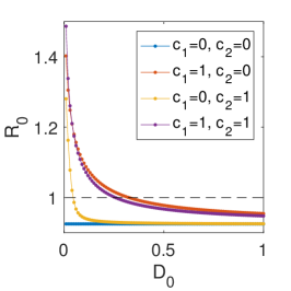
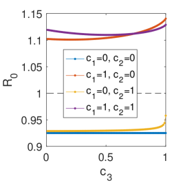
Figure 4: The impact of spatial heterogeneity on reproduction number. (A) For fixed $[\beta]$, $R_{0}$ is minimized for the homogeneous case; similarly for fixed $[\alpha]$. (B) When $\beta$ and $\alpha$ are spatially homogeneous (i.e. $\beta=[\beta]$ and $\alpha=[\alpha]$), the baseline level of diffusion, $D_{0}$, has no impact on $R_{0}$. $D(x)=D_{0}(1+\cos(\pi x))$; see text for other parameters. (C) When $\beta$ and $\alpha$ are spatially homogeneous, the level of spatial heterogeneity of diffusion has no impact on $R_{0}$. $D(x)=0.0685(1+c_{3}\cos(\pi x))$; see text for other parameters.

We next reproduce some of Wang and Zhao’s numerical results. One such finding concerns the impact of spatial heterogeneity; in particular that $\mu_{1}\leq\bar{\mu}_{1}$, where ${\mu}_{1}$ is the principal eigenvalue of their associated eigenvalue problem, and $\bar{\mu}_{1}$ is the principal eigenvalue where $\beta$ and $\alpha$ are replaced by their spatial averages (this is Lemma 4.4 in [18]). Since $R_{0}=1/\mu_{1}$, this means that $R_{0}$ is minimized for the spatially homogeneous problem. We used the constant parameters: $a=0.0027$, $\alpha=0.2$, $\sigma=0.0357$, $K=0.98$. Then $\beta(x)=0.2192(1+c_{1}\cos(\pi x))$. Fig. 4A shows that $R_{0}$ is minimized when $c_{1}=0$. Similarly, restoring $\beta=0.2192$ and varying $\alpha(x)=0.2(1+c_{2}\cos(\pi x))$, $R_{0}$ is minimized for the spatially homogenous case.

We next look at the effect of varying $D_{0}$, the baseline diffusion coefficient, when spatial heterogeneity in $\beta$ and/or $\alpha$ are present. To get a fair comparison for the role of heterogeneity, we used $\beta(x)=0.2192(1+c_{1}\cos(\pi x))$ and $\alpha(x)=\frac{2}{\pi}(1+c_{2}\left(\sin(\pi x)-\frac{2}{\pi})\right)$, so that $[\alpha]$ is preserved as $c_{2}$ changes; the variable diffusion is: $D(x)=D_{0}(1+\cos(\pi x))$. Remarkably, $D_{0}$ has no effect on $R_{0}$ when both $\beta$ and $\alpha$ are constant.

We can also vary the modulation magnitude of the diffusion, i.e. allow $D(x)=0.0685(1+c_{3}\cos(\pi x))$, where $c_{3}$ is varied. Wang found that again $R_{0}$ is constant when $\beta$ and $\alpha$ are spatially homogeneous. We confirm this in Fig. 4C, again including heterogeneity in either $\beta$, or $\alpha$, both, or neither.

Wang and Zhao next considered the problem of designing a vaccine strategy, based on the hypothesis that the impact of the vaccine could be modeled by changes to disease transmission $\beta(x)$. They suppose that

$$\beta(x)=6x(1-x)$$

and consider how $R_{0}$ would change if we modified

$$\beta\rightarrow\beta\frac{1}{1+v_{0}(x)}$$

where

$$v_{0}(x)=\left\{\begin{matrix}\frac{c_{0}}{L}&0\leq a_{0}\leq x<a_{0}+L\leq 1\\ 0&{\rm otherwise}\end{matrix}\right.$$

The authors interpret $\frac{v_{0}}{1+v_{0}}=1-\frac{1}{1+v_{0}}$ as the vaccine efficacy. The spatial function can be motivated by the idea of distributing a total quantity of $c_{0}$ over an area of size $L$, beginning at $a_{0}$.

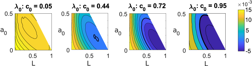
Figure 5: Optimizing a vaccine strategy to control rabies. Principal eigenvalue $\lambda_{0}$, indicating whether an initial infection will spread ($\lambda_{0}>0$) or dissipate ($\lambda_{0}<0$). In each panel, $c_{0}$ is fixed while $a_{0}$ and $L$ are varied. From left to right: $c_{0}=0.05,0.44,0.72,0.95$.

To understand the impact of a vaccine strategy, we solved Eqn. (38) by sweeping over the parameters $c_{0}$, $a_{0}$ and $L$. We surveyed $0\leq c_{0},L\leq 1$; by symmetry of $\beta(x)$ it suffices to consider $0\leq a_{0}\leq 0.5$, and we limited our consideration to $a_{0}+L\leq 1$. Other parameters were as used previously: $a=0.0027$, $b=a/2$, $\sigma=0.0357$, $K=1.5$, $\alpha(x)=\alpha_{0}=0.2$, $D(x)=D_{0}=0.1371$.

First, we can ask how much vaccine is required to prevent an epidemic; i.e. how large does $c_{0}$ need to be for $\lambda_{0}<0$. Not surprisingly, $\lambda_{0}$ decreases with $c_{0}$; the minimum value of $c_{0}$ for which stability was observed was $0.44$. However, stability also depends strongly on where the vaccine is used, as well as its spatial distribution: in Fig. 5 we show $\lambda_{0}$ as a function of $a_{0}$ and $L$, for selected values of $c_{0}$: for $c_{0}\geq 0.44$ (three rightmost panels), the boundary of the stable region is shown as bold. Note that even for the largest vaccine quantity tested ($c_{0}=0.95$), a suboptimal distribution strategy can easily fail to contain the infection (i.e. $\lambda_{0}>0$).

Finally, we can examine the optimal vaccine strategy — the configuration that minimizes $\lambda_{0}$, given a total quantity $c_{0}$. For the values of $c_{0}$ shown in Fig. 5, we found the $(a_{0},L)$ values at which $\lambda_{0}$ was minimized, and show the corresponding vaccine strategy and its effect on the disease transmission rate (i.e. the modified $\beta(x)$) in Fig. 6. In all cases, the optimal strategy is symmetric; the vaccine should always be distributed on the area where $\beta$ is largest.

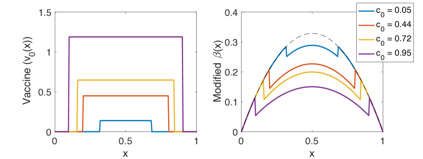
Figure 6: The optimal vaccine strategy to control rabies, given a total quantity of available vaccine $c_{0}$. Left panel: The optimal strategy obtained by minimizing over dispersal location $a_{0}$ and dispersal area $L$. Right panel: the resulting disease transmission coefficient, showing a decrease in the dispersal area. For reference, $\beta(x)$ with no vaccine is shown (black dashed line).

Appendix A Proof of the Sturm oscillation theorem for rational Herglotz pencils

We give a short proof of the Sturm property for the rational Herglotz pencil problem

$$-\partial_{x}(D(x)p_{x})=\left(-V(x)+\sum_{i=1}^{N}\frac{\beta_{i}(x)}{\lambda-\alpha_{i}}+\lambda\right)p=g(x,\lambda)p\qquad p_{x}(a)=0=p_{x}(b)$$

We take the convention that $\alpha_{0}=-\infty$ and $\alpha_{N+1}=+\infty$. Then in each interval $(\alpha_{j-1},\alpha_{j}),~{}~{}~{}j\in\{1\ldots N\}$ there exists a strictly increasing sequence of (real) eigenvalues $\{\lambda^{j}_{k}\}_{k=0}^{\infty}\in(\alpha_{j-1},\alpha_{j})$ whose only accumulation point is $\alpha_{j}$ such that the eigenfunction $\phi_{k}^{j}(x)$ has exactly $k$ (simple) roots in the interval $(a,b)$. The exact boundary conditions used are not particularly important – the same basic arguments work with Dirichlet, Robin or (with some additional modifications) periodic boundary conditions – but we work with Neumann boundary conditions since these are most appropriate for the models considered here.

The easiest way to prove the Sturm theorem is via the Prüfer angle, a change of variable for the second order linear differential equation defined by

(40) $$p(x,\lambda)=R(x,\lambda)\cos(\Theta(x,\lambda))$$

(41) $$p_{x}(x,\lambda)=R(x,\lambda)\sin(\Theta(x,\lambda)).$$

It is well-known (at least to those that well-know it) that if $p(x,\lambda)$ satisfies the second order equation

$$-\partial_{x}(D(x)p_{x})=g(x,\lambda)p$$

then the Prüfer angle $\Theta(x,\lambda)$ satisfies the equation

(42) $$\Theta_{x}=-\sin^{2}\Theta-g(x,\lambda)\cos^{2}\Theta-\frac{D_{x}R}{D}\sin\Theta\cos\Theta$$

while the radial function $R(x,\lambda)$ satisfies the equation

(43) $$R_{x}=\left(1-\frac{g}{D}\right)R\sin(\Theta)\cos(\Theta)-\frac{D_{x}}{D}R\sin^{2}\Theta.$$

We will mostly work with the angle $\Theta(x,\lambda)$: the radial function $R(x,\lambda)$ is important only insofar as equation (43) shows that $R(x,\lambda)$ cannot vanish unless it is identically zero, implying that the Prüfer coordinate change is well-defined for all $x$.

The basic idea of the proof is that the winding of the Prüfer angle is a good measure of the winding of the eigenfunctions, and that this can be understood via equations (40, 41). Since $R(x,\lambda)$ cannot vanish, the roots of $p$ correspond to places where $\Theta(x,\lambda)=k\pi$ while critical points of $p$ correspond to places where $\Theta(x,\lambda)=(k+\frac{1}{2})\pi$. We will look in particular at the solution to (42) satisfying the initial condition $\Theta(a,\lambda)=0$ (and, for concreteness sake, $R(a,\lambda)=1$), so that the corresponding $p$ satisfies $p(a,\lambda)=1,p_{x}(a,\lambda)=0.$ In this setting eigenvalues will correspond to values of $\lambda=\lambda^{*}$ such that $\Theta(b,\lambda^{*})=k\pi.$

We note several facts. First note that, for fixed values of $x$ the function $\Theta(x,\lambda)$ is a decreasing function of $\lambda$. This follows from differentiating equation 42 with respect to $\lambda$, using the fact that $\frac{dg}{d\lambda}>0$ and applying the Gronwall inequality. Next we note that, for $\lambda$ sufficiently close to $\alpha_{j-1}^{+},$ $\Theta(x,\lambda)$ must satisfy $0\leq\Theta(x,\lambda)<\frac{\pi}{2}$, with $\Theta(x,\lambda)=0$ if and only if $x=0$. To see this note that we can choose $\lambda$ close enough to $\alpha_{j-1}$ to guarantee that $g(x,\lambda)<0$. In this case we have that $\Theta_{x}|_{\Theta=0}>0$ and $\Theta_{x}|_{\Theta=\frac{\pi}{2}}<0$. This guarantees that the interval $\Theta\in(0,\frac{\pi}{2})$ is invariant in positive $x$. Finally note that, if $\Theta=-(k+\frac{1}{2})\pi$ then $\Theta_{x}=-1$, so the curve $\Theta(x,\lambda)$ always crosses the line $-(k+\frac{1}{2})\pi$ transversely and in the same direction.

The proof now follows from considering a homotopy in $\lambda$: we begin with the curve $\Theta(x,\lambda)$ with $\lambda$ sufficiently close to $\alpha_{j-1}$ so that $\Theta(x,\lambda)$ lies in the interval $(0,\frac{\pi}{2})$. Thus no value of $\lambda$ in this range can be an eigenvalue since $\Theta(b,\lambda)$ is strictly between $0$ and $\frac{\pi}{2}$, so we are below the spectrum.

Next we consider increasing $\lambda$, which will decrease $\Theta(b,\lambda)$. The first eigenvalue occurs when $\Theta(b,\lambda)=0.$ Call this value $\lambda_{0}$. While we do not know much about the shape of the curve $\Theta(x,\lambda_{0})$ we do know that it cannot cross the line $\Theta=-\frac{\pi}{2}$ since at any point where $\Theta(x,\lambda)=-(k+\frac{1}{2})\pi$ we have that $\Theta_{x}=-1$. Hence as $\lambda$ is increased the first time that the curve $\Theta(x,\lambda)$ can cross the line $\Theta=-(k+\frac{1}{2})\pi$ must be at the endpoint $x=b$.

This pattern continues as $\lambda$ increases: $\Theta(b,\lambda)$ decreases and alternately crosses the lines $\Theta=-k\pi$ and $\Theta=-(k+\frac{1}{2})\pi$: the former correspond to eigenvalues and at the latter $p(x,\lambda)$ picks up a root. Since $R(x,\lambda)$ is non-vanishing and $\Theta$ and $\Theta_{x}$ cannot vanish simultaneously it follows that the $k^{th}$ eigenfunction has exactly $k$ roots in $(a,b)$. It follows from standard estimate that away from poles of $g(x,\lambda)$ we have analytic dependence of $\Theta(b,\lambda)$ on $\lambda$ and so solutions to $\Theta(b,\lambda)=-(k+\frac{1}{2})\pi$ must be isolated. It is also clear that by choosing $\lambda$ sufficiently close to $\alpha_{j}$ we can guarantee that $\Theta_{x}$ is uniformly large and negative, and thus that $\alpha_{j}$ is an accumulation point of eigenvalues.

Appendix B Numerical Methods

We use standard methods to solve the eigenvalue problem:

(44) $$Hu+q(x)u+\sum_{i=1}^{N}\frac{\beta_{i}(x)u}{\lambda-\alpha_{i}} = \lambda u;\;0\leq x\leq L$$

where $H$ is a Sturm-Liouville operator, such as the second derivative (i.e. $Hu=-u_{xx}$). We assume that $\beta_{i}(x)>0$ on the domain $[0,L]$ and that boundary conditions are of the typical kind:

(45) $$b^{0}_{0}u(0)+b^{1}_{0}\frac{\partial u}{\partial x}(0) = 0$$

(46) $$b^{0}_{L}u(L)+b^{1}_{L}\frac{\partial u}{\partial x}(L) = 0$$

where $b^{0}_{0}\not=0$ and/or $b^{1}_{0}\not=0$, and $b^{0}_{L}\not=0$ and/or $b^{1}_{L}\not=0$. Introducing auxiliary functions $v^{(i)}=\frac{\beta_{i}(x)u}{\lambda-\alpha_{i}}$, we find that Eqn. (44) is equivalent to

(47) $$Hu+q(x)u+\sum_{i=1}^{N}v^{(i)} = \lambda u;$$

(48) $$\beta_{i}(x)u+\alpha_{i}v^{(i)} = \lambda v^{(i)},\,i=1,...,N$$

We used standard second-order discretizations to evaluate $Hu$ at $n_{x}-1$ interior points of $[0,L]$; e.g. centered differencing for $Hu=-u_{xx}$. For the spatially variable diffusion in §4, we used the stencil

$$(D(x)u_{x})_{x} \approx \frac{1}{(\Delta x)^{2}}(D_{i-1/2}u_{i-1}-(D_{i-1/2}+D_{i+1/2})u_{i}+D_{i+1/2}u_{i+1})$$

where $x_{i}=i\Delta x$, $u_{i}=u(x_{i})$, $D_{i-1/2}=D(x_{i-1/2})$, etc.; i.e. the diffusion function is evaluated at half-intervals.

Finally, the boundary conditions are incorporated with the second-order stencils

$$\frac{\partial u}{\partial x}(0)\approx\frac{-3u_{0}+4u_{1}-u_{2}}{2\Delta x};\qquad\frac{\partial u}{\partial x}(L)\approx\frac{3u_{n_{x}}-4u_{n_{x}-1}+u_{n_{x}-2}}{2\Delta x};$$

This results in a linear system of size $(N+1)(n_{x}-1)$, representing the unknown functions $u$ and $v_{i}$ at each of $n_{x}-1$ interior points; we numerically approximate its eigenvalues using standard methods (we used the eig function from Matlab R2017b).

Here, we list parameters used for specific cases in the paper.

• In Example 3.4, we used $L=\pi$ and $n_{x}=100$; i.e. $\Delta x=\pi/n_{x}$ and the number of interior points is $n_{x}-1=99$. For Figure 3, we repeated the computations with $n_{x}=200$ and $n_{x}=400$.

• For all computations presented in §4, $L=1$ and $n_{x}=200$.

References

- [1] V. Adamjan, H. Langer, and M. Langer. A spectral theory for a -rational Sturm-Liouville problem. J. Differential Equations, 171(2):315–345, 2001.
- [2] V. Capasso and R. E. Wilson. Analysis of a reaction-diffusion system modeling man-environment-man epidemics. SIAM Journal on Applied Mathematics, 57(2):327 – 346, 1997.
- [3] M. P. Drazin and E. V. Haynsworth. Criteria for the reality of matrix eigenvalues. Math. Z., 78:449–452, 1962.
- [4] Z. Feng, W. Huang, and D. L. DeAngelis. Spatially heterogeneous invasion of toxic plant mediated by herbivory. Mathematical Biosciences and Engineering, 10:1519 – 1538, 2013.
- [5] A. Ghazaryan, Y. Latushkin, and S. Schecter. Stability of travelling waves for a class of reaction-diffusion systems that arise in chemical reaction models. SIAM Journal on Mathematical Analysis, 42:2434–2472, 2010.
- [6] Y. Ghazaryan, A. andLatushkin, S. Schecter, and A. J. de Souza. Stability of gasless combustion fronts in one-dimensional solids. Archive for Rational Mechanics and Analysis, 198(3):981–1030, Dec 2010.
- [7] T. Kapitula and K. Promislow. Stability indices for constrained self-adjoint operators. Proceedings of the American Mathematical Society, 140:865–880, 2012.
- [8] D. J. Kaup and A. C. Newell. An exact solution for a derivative nonlinear schrödinger equation. Journal of Mathematical Physics, 19(4):798–801, 1978.
- [9] R. Kollar and P. D. Miller. Graphical krein signature theory and evans-krein functions. SIAM Review, 56:73–123, 2014.
- [10] M.A. Lewis. Spatial coupling of plant and herbivore dynamics: the contribution of herbivore dispersal to transient and persistent waves of damage. Theoretical Population Biology, 45:277–312, 1994.
- [11] Y. Lou, Q. Nie, and F. Y. M. Wan. Nonlinear eigenvalue problems in the stability analysis of morphogen gradients. Studies in Applied Mathematics, 113:183–215, 2004.
- [12] W. F. Morris and G. Dwyer. Population consequences of constitutive and inducible plant resistance: herbivore spatial spread. The American Naturalist, 149:1071–1090, 1997.
- [13] J. D. Murray, E. A. Stanley, and D. L. Brown. On the spatial spread of rabies among foxes. Proceedings of the Royal Society of London B, 229:111–159, 1986.
- [14] F. Sánchez-Garduno and V. F. Brena-Medina. Seaching for spatial patterns in a pollinator-plant-herbivore mathematical model. Bulletin of Mathematical Biology, 73:1118–1153, 2011.
- [15] B. Simon. Orthogonal polynomials on the unit circle. American Mathematical Soc., 2005.
- [16] L. A. Takhtajan and L. D. Faddeev. Essentially nonlinear one-dimensional model of classical field theory. Theoretical and Mathematical Physics, 21(2):1046–1057, Nov 1974.
- [17] P. van den Driessche and J. Watmough. Reproduction numbers and sub-threshold endemic equilibria for compartmental model of disease transmission. Mathematical Biosciences, 180:29–48, 2002.
- [18] W. Wang and X.-Q. Zhao. Basic reproduction numbers for reaction-diffusion epidemic models. SIAM Journal of Applied Dynamical Systems, 11(4):1652–1973, 2012.