High resolution spectroscopy of the relatively hydrogen-poor
metal rich giants in the globular cluster $\omega$ Centauri

Abstract

High-resolution optical spectra are analyzed for two of the four metal rich mildly hydrogen-poor or helium-enhanced giants discovered by Hema & Pandey (2014) along with their comparison normal (hydrogen-rich) giants. The strengths of the MgH bands in the spectra of the program stars are analyzed for their derived stellar parameters. The observed spectra of the sample (hydrogen-poor) stars (LEID 39048 and LEID 34225) show weaker MgH bands unlike in the spectra of the normal comparison giants (LEID 61067 and LEID 32169). The magnesium abundance derived from MgH bands is less by 0.3 dex or more for LEID 39048 and LEID 34225, than that derived from Mg i lines. This difference, cannot be reconciled by making the changes to the stellar parameters within the uncertainties. This difference in the magnesium abundances derived from Mg i lines and from the MgH band is unacceptable. This difference is attributed to the hydrogen-deficiency or helium-enhancement in their atmospheres. These metal rich hydrogen-poor or helium-rich giants provide an important link to the evolution of the metal-rich sub population of $\omega$ Cen. These stars provide the first direct spectroscopic evidence for the presence of the He-enhancement in the metal rich giants of $\omega$ Cen.

1 Introduction

The brightest and the most massive Galactic globular cluster (GGC) $\omega$ Cen exhibits a large spread in metallicity ([Fe/H)] and other abundance anomalies among the cluster stars (Johnson & Pilachowski, 2010; Simpson & Cottrell, 2013; Sollima et al., 2005) including the existence of multiple stellar population with the cluster dwarfs/giants having normal helium, and enhanced helium or relatively hydrogen-poor (H-poor) atmospheres (Piotto et al., 2005; Villanova et al., 2007; Dupree & Avrett, 2013).

The doubt is that these relatively H-poor or He-rich giants appear metal rich, than they really are, due to the lower continuum absorption. Note that the spectra of H-poor F- and G-type supergiants, R Coronae Borealis (RCB) and the H-deficient carbon (HdC) stars, appear metal rich when compared with the spectra of normal F- and G-type supergiants (Pandey et al., 2004). This is ascribed to the lower continuum opacity in the atmosphere due to H-deficiency. Hence, these stars appear more metal rich than they actually are (Sumangala Rao et al., 2011). The origin and evolution of these enigmatic stars, RCB/HdC, are not yet clear due to their rarity and chemical peculiarity.

A low resolution optical spectroscopic survey was conducted among the giants of $\omega$ Cen for idetifying new R Coronae Borealis (RCB) stars (Hema & Pandey, 2014). Identifying RCB stars in a globular cluster gives an idea of their position on the HR-diagram and is a potential clue to understand their origin and evolution.

Hema & Pandey (2014) survey resulted in the discovery of four mildly H-deficient giants in $\omega$ Cen. For two out of these four giants, high resolution spectra were obtained along with their comparison stars with similar stellar parameters as these two giants. In this paper we have conducted a detailed high resolution spectroscopic analyses for two mildly H-deficient giants along with their comparison stars to confirm their H-deficiency or the He-enhancement.

2 Observations and data reduction

The high-resolution optical spectra were obtained using Southern African Large Telescope (SALT) $-$ high resolution spectrograph (HRS). These spectra obtained with the SALT-HRS are having a resolving power, R ($\lambda$/$\Delta$$\lambda$) of 40000. The spectra were obatined with both blue and red camera using 2K $\times$ 4K and 4K $\times$ 4K CCDs, respectively, spanning a spectral range of 370$-$550 nm in the blue and 550$-$890 nm in the red.

The spectral reductions were carried out using the IRAF software. The traditional data reduction procedure including, bias subtraction, flat field correction, spectrum extraction, wavelength caliberation, etc. were followed.

The extracted and wavelength calibrated 1d spectra were continuum normalized. The region of the spectrum with maximum flux points and free of absorption lines were considered for continuum fitting with a smooth curve passing through these points. To improve the signal-to-noise, the observed spectra of the program stars were smoothed such that the strength of the spectral lines are not altered. The signal-to-noise ratio per pixel of the smoothed blue spectra of the program stars at about 5000Å is $\sim$ 150 and for red spectra at about 7000Å is $\sim$ 200. Since there is a overlap of wavelengths, the spectrum is continuous without gaps in the blue and red spectral range. The atlas of high-resolution spectrum of Arcturus (Hinkle et al., 2000) was used as a reference for continuum fitting and also for identifying the spectral lines.

3 Abundance Analysis

In order to conduct a detailed abundance analysis, the equivalent widths for weak and strong lines of several elements, that are clean and also not severely blended for both neutral and ionized states were meaured using different commands in IRAF.

The wavelength calibrated spectrum of a program star (LEID 39048) was used to measure the shift of the spectral lines from the rest wavelengths; Hinkle et al. (2000)’s atlas of Arcturus was used as reference. Adopting LEID 39048’s spectrum as a template, the radial velocities and the uncertainties involved were determined for other program stars using the task $fxcor$ in IRAF. Then the heliocentric corrections were applied to these radial velocities. The heliocentric velocities for the program stars are given in Table 1, and are in good agreement with the mean velocity of the cluster, $V_{r}$ = 233 km s^-1, with the dispersion ranging from 15 to 6 km s^-1 from center to outwards, respectively (Mayor et al., 1997).

For determination of stellar parameters and the elemental abundances, the LTE line analysis and spectrum synthesis code MOOG (Sneden, 1973) and the ATLAS9 (Kurucz, 1998) plane parallel, line-blanketed LTE model atmospheres were used.

The microturbulence ($\xi_{t}$) is derived using Fe i lines having similar excitation potential and a range in equivalent width, weak to strong, giving the same abundance. The effective temperature ($T_{\rm eff}$) is determined using the excitation balance of Fe i lines having a range in lower excitation potential. The $T_{\rm eff}$ and $\xi_{t}$ were fixed iteratively. The process was carried out untill both returned zero slope.

By adopting the determined $T_{\rm eff}$ and $\xi_{t}$, the surface gravity (log $g$) is derived. The surface gravity is fixed by demanding the same abundances from the lines of different ionization states of a species, known as ionization balance. The surface gravity is derived using the lines of Fe i/Fe ii, Ti i/Ti ii, and Sc i/Sc ii. Then the mean log $g$ was adopted.

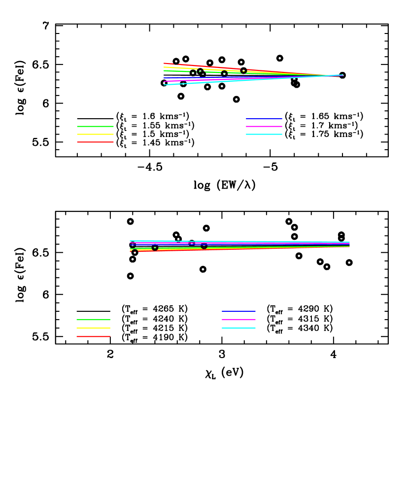
Figure 2: Figure shows the estimation of uncertainties on $T_{\rm eff}$ (lower panel) and $\xi_{t}$ (upper panel). The adopted stellar parameters for deriving $\Delta$$T_{\rm eff}$ and $\Delta$$\xi_{t}$ are, ($T_{\rm eff}$, log $g$, $\xi_{t}$): (4265 K, 1.3 cgs units, 1.6 kms^-1). The adopted uncertainties corresponding to the 1$\sigma$ error on the abundance of the zero slope are $\Delta$$T_{\rm eff}$ = $\pm$50 K and $\Delta$$\xi_{t}$ = 0.1kms^-1. See figure for the keys.

Uncertainty on the $T_{\rm eff}$ and $\xi_{t}$ is estimated by changing the $T_{\rm eff}$ in steps of 25K and $\xi_{t}$ in steps of 0.05 km s^-1. The change in $T_{\rm eff}$ and $\xi_{t}$ and the corresponding change, in the mean abundances from the the mean abundances (of zero slope), of about 1$\sigma$ error on the the mean abundances (of zero slope) is obtained. This change is adopted as the uncertainty on these parameters. The adopted $\Delta$$T_{\rm eff}$ = $\pm$50 K and $\Delta$$\xi_{t}$ = $\pm$0.1 km s^-1 (see Figure 2). The uncertainties on log $g$ is the standard deviation from the mean value of the log $g$ determined from different species, which is about $\pm$0.1 (cgs units). The adopted stellar parameters with the uncertainties are given in Table 1.

The log $g$ values for the program stars in Hema & Pandey (2014) were derived using the standard relation:

log(g_∗) $=$ 0.40($M_{\rm bol.}$ $-$ $M_{\rm bol,\odot}$) $+$ log($g_{\odot}$) $+$ 4(log($T$/$T_{\odot}$)) $+$ log($M$/$M_{\odot}$) — Eq (1)

The bolometric correction to $M_{v}$ was applied using the relation given by Alonso et al. (1999). The distance modulus for $\omega$ Cen, $(m-M)_{v}$ = 13.7, and the mass of $\omega$ Cen red giants were assumed to be 0.8$M_{\odot}$ (Johnson & Pilachowski, 2010). Using the photometric temperatures derived from ${(J-H)_{0}}$, ${(J-K)_{0}}$ and $(b-y)$ colours in Equation (1) the log $g$ values were derived.

The difference in the log $g$ values derived by us and those derived by Johnson & Pilachowski (2010) are within $\pm$0.1 (cgs units). Hence, the uncertainty on the log $g$ values adopted by Hema & Pandey (2014) was about $\pm$0.1 (cgs units) (for details see Hema & Pandey (2014)).

Color-magnitude diagram for our program stars and for the sample red giants of Johnson & Pilachowski (2010) is given in figure 1.

Table 1: Photometric and spectroscopic parameters for the program stars.

Parameters	LEID 34225	LEID 39048	LEID 61067	LEID 32169
RA	13 27 53.7	13 26 3.9	13 26 50.7	13 27 33.2
Declination	-47 24 43.3	-47 26 54.1	-47 37 1.0	-47 23 47.9
Visual Magnitude (V)	13.0	12.8	12.5	13.3
$B-V$	1.23	1.42	1.60	1.17
Metallicity([Fe/H])	-1.0	-0.65	-1.0	-1.0
Vhelio	235$\pm$0.5	238$\pm$0.5	230$\pm$0.5	230$\pm$0.5
Date of Observation	2016 May 27	2016 May 3	2016 May 15	2016 June 25
$T_{\rm eff}$	4275$\pm$50	3965$\pm$50	4040$\pm$50	4285$\pm$50
log $g$	1.30$\pm$0.1	0.95$\pm$0.1	0.85$\pm$0.1	1.35$\pm$0.1
$\xi$	1.6$\pm$0.1	1.6$\pm$0.1	1.6$\pm$0.1	1.6$\pm$0.1
$T_{\rm eff}$	4265$\pm$50	3965$\pm$50	4035$\pm$50	4285$\pm$50
log $g$	1.30$\pm$0.15	0.95$\pm$0.15	0.85$\pm$0.15	1.35$\pm$0.15
$\xi$	1.6$\pm$0.2	1.6$\pm$0.2	1.6$\pm$0.2	1.6$\pm$0.2
$T_{\rm eff}$	4266$\pm$50	3945$\pm$50	4010$\pm$50	4260$\pm$50
log $g$	1.35$\pm$0.1	1.0$\pm$0.1	0.95$\pm$0.1	1.4$\pm$0.1

^a This work
^b From Johnson & Pilachowski (2010)
^c Photometric determinations from Hema & Pandey (2014)

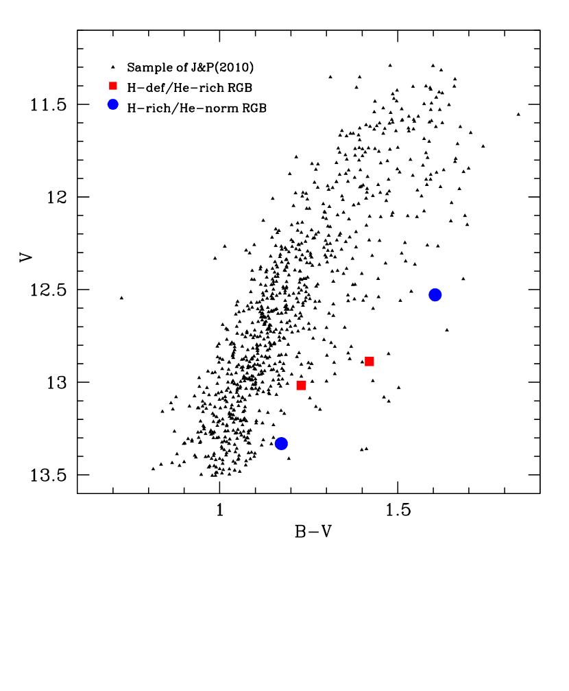
Figure 1: Figure shows the Color-magnitude diagram for our sample $\omega$ Cen red giants along with the sample red giants from Johnson & Pilachowski (2010). All the photometric data are from Johnson & Pilachowski (2010). The filled red squares are the H-deficient/He-enhanced giants and the filled blue circles are the normal giants of our sample. The filled black triangles are the sample red giants of Johnson & Pilachowski (2010). See figure for the keys.

Table 2: The linelist used for the abundance analysis of the program stars. The table gives the wavelength (Å), lower excitation potentail (eV), transition probabilities (log $gf$), and the measured equivalent widths/log $\epsilon$(E) for that line, for different species.

Wavelength	$\chi$(eV)	log $gf$	LEID 34225	LEID 39048	LEID61067	LEID32169
(Å)	(eV)		(mÅ)/log $\epsilon$(E)	(mÅ)/log $\epsilon$(E)	(mÅ)/log $\epsilon$(E)	(mÅ)/log $\epsilon$(E)
O i $\lambda$6300.31	0.00	$-$9.75	13/7.40	43/8.06	33/5.65	21/7.71
O i $\lambda$6363.78	0.02	$-$10.19	$\cdots$	21/8.15	$\cdots$	10/7.81
Mean (log $\epsilon$(O i))	$\cdots$	$\cdots$	7.4	8.1$\pm$0.06	7.73	7.76$\pm$0.07
Na i $\lambda$4751.82	2.10	$-$2.08	26/5.73	$\cdots$	79/6.46	34/5.91
Na i $\lambda$5148.84	2.10	$-$2.04	39.7/5.93	$\cdots$	76/6.31	41/5.96
Na i $\lambda$6154.23	2.10	$-$1.57	58/5.67	134/6.53	122/6.42	79/6.00
Na i $\lambda$6160.75	2.10	$-$1.27	70/5.55	149/6.47	142/6.44	98/5.97
Mean (log $\epsilon$(Na i))	$\cdots$	$\cdots$	5.72$\pm$0.16	6.50$\pm$0.04	6.40$\pm$0.07	5.96$\pm$0.04
Mg i $\lambda$4730.04	4.34	$-$2.39	$\cdots$	97/7.27	89/7.10	$\cdots$
Mg i $\lambda$5711.09	4.34	$-$1.73	105/6.70	145/7.35	121/6.86	115/6.88
Mg i $\lambda$6318.72	5.11	$-$1.73	40/6.60	83/7.52	69/7.01	39/6.61
Mg i $\lambda$6319.24	5.11	$-$1.95	29/6.61	49/7.43	56/7.01	34/6.74
Mg i $\lambda$7657.61	5.11	$-$1.28	78/6.70	126/7.47	106/7.05	85/6.81
Mean (log $\epsilon$(Mg i))	$\cdots$	$\cdots$	6.65$\pm$0.05	7.41$\pm$0.1	7.00$\pm$0.1	6.80$\pm$0.14
Al i $\lambda$6696.03	3.14	$-$1.57	100/6.37	119/6.37	110/6.30	79/6.05
Al i $\lambda$6698.67	3.14	$-$1.89	89/6.49	103/6.42	90/6.30	66/6.14
Al i $\lambda$7835.31	4.02	$-$0.64	93/6.66	99/6.56	73/6.23	59/6.15
Al i $\lambda$7836.13	4.02	$-$0.49	91/6.47	115/6.65	108/6.59	75/6.24
Mean (log $\epsilon$(Al i))	$\cdots$	$\cdots$	6.50$\pm$0.12	6.50$\pm$0.13	6.35$\pm$0.16	6.15$\pm$0.08
Si i $\lambda$5684.48	4.95	$-$1.65	58/6.91	71/7.45	59/7.01	48/6.76
Si i $\lambda$5690.42	4.93	$-$1.87	47/6.92	50/7.22	67/7.35	50/6.98
Si i $\lambda$5701.10	4.93	$-$2.05	48/7.11	40/7.19	41/7.03	31/6.79
Si i $\lambda$5772.15	5.08	$-$1.75	57/7.16	62/7.54	58/7.28	46/6.97
Si i $\lambda$5793.07	4.93	$-$2.06	41/6.97	56/7.52	54/7.29	$\cdots$
Si i $\lambda$6155.13	5.62	$-$0.78	$\cdots$	75/7.20	81/7.08	66/6.68
Si i $\lambda$6237.32	5.61	$-$1.28	$\cdots$	80/7.41	74/7.07	69/6.85
Mean (log $\epsilon$(Si i))	$\cdots$	$\cdots$	7.00$\pm$0.11	7.36$\pm$0.15	7.16$\pm$0.14	6.84$\pm$0.12
Ca i $\lambda$5260.39	2.52	$-$1.90	50/5.59	$\cdots$	78/5.82	57/5.73
Ca i $\lambda$5867.56	2.93	$-$0.80	60/5.17	$\cdots$	89/5.42	89/5.68
Ca i $\lambda$6161.29	2.52	$-$1.28	83/5.20	143/5.85	140/5.89	98/5.47
Ca i $\lambda$6162.18	1.90	$-$0.07	$\cdots$	345/5.88	295/5.58	233/5.41
Ca i $\lambda$6166.44	2.52	$-$1.11	96/5.31	158/6.00	135/5.69	106/5.49
Ca i $\lambda$6169.04	2.52	$-$0.69	122/5.43	168/5.80	146/5.53	125/5.47
Ca i $\lambda$6169.56	2.53	$-$0.27	135/5.39	191/5.85	171/5.66	142/5.50
Ca i $\lambda$6455.60	2.52	$-$1.34	90/5.62	137/6.01	111/5.66	95/5.70
Ca i $\lambda$6471.66	2.53	$-$0.59	126/5.50	172/5.84	151/5.59	136/5.67
Ca i $\lambda$6499.65	2.52	$-$0.59	124/5.45	176/5.88	$\cdots$	134/5.61
Mean (log $\epsilon$(Ca i))	$\cdots$	$\cdots$	5.40$\pm$0.16	5.9$\pm$0.08	5.65$\pm$0.14	5.57$\pm$0.12
Sc i $\lambda$4743.82	1.45	0.07	$\cdots$	$\cdots$	91/2.34	$\cdots$
Sc i $\lambda$5081.56	1.45	0.06	$\cdots$	$\cdots$	79/2.10	$\cdots$
Sc i $\lambda$5484.63	1.85	0.08	20/2.47	$\cdots$	32/2.38	$\cdots$
Sc i $\lambda$5671.83	1.45	0.64	69/2.22	$\cdots$	101/2.32	59/2.08
Sc i $\lambda$6210.67	0.00	$-$1.53	58/2.08	$\cdots$	100/2.05	69/2.27
Sc i $\lambda$6305.66	0.02	$-$1.30	85/2.17	$\cdots$	138/2.36	67/1.97
Mean (log $\epsilon$(Sc i))	$\cdots$	$\cdots$	2.24$\pm$0.16	$\cdots$	2.26$\pm$0.14	2.10$\pm$0.15
Sc ii $\lambda$5357.20	1.51	$-$2.21	19/2.36	$\cdots$	17/2.21	18/2.38
Sc ii $\lambda$5552.23	1.46	$-$2.28	$\cdots$	$\cdots$	32/2.57	18/2.36
Sc ii $\lambda$5684.21	1.51	$-$1.07	74/2.29	69/2.28	72/2.16	56/2.00
Sc ii $\lambda$6245.62	1.51	$-$0.98	80/2.27	95/2.60	86/2.25	60/1.97
Sc ii $\lambda$6300.75	1.51	$-$1.84	29/2.19	49/2.67	35/2.23	31/2.28
Sc ii $\lambda$6320.84	1.50	$-$1.77	30/2.14	45/2.51	38/2.19	$\cdots$
Sc ii $\lambda$6604.58	1.36	$-$1.48	$\cdots$	96/2.85	79/2.39	$\cdots$
Mean (log $\epsilon$(Sc ii))	$\cdots$	$\cdots$	2.25$\pm$0.09	2.60$\pm$0.2	2.28$\pm$0.14	2.20$\pm$0.2
Ti i $\lambda$5219.70	0.02	$-$2.29	140/4.49	200/4.93	185/4.84	$\cdots$
Ti i $\lambda$5295.77	1.07	$-$1.63	93/4.44	141/4.82	120/4.47	78/4.18
Ti i $\lambda$5490.15	1.46	$-$0.93	99/4.38	$\cdots$	129/4.48	87/4.17
Ti i $\lambda$5702.66	2.30	$-$0.44	$\cdots$	99/4.54	67/4.10	31/3.86
Ti i $\lambda$5716.44	2.30	$-$0.72	34/4.20	86/4.59	70/4.44	30/4.15
Ti i $\lambda$6092.79	1.89	$-$1.32	$\cdots$	$\cdots$	56/4.18	25/4.06
Ti i $\lambda$6146.23	1.87	$-$1.51	$\cdots$	$\cdots$	70/4.17	22/3.78
Ti i $\lambda$6258.11	1.44	$-$0.38	$\cdots$	197/4.75	161/4.20	105/3.74
Ti i $\lambda$6261.10	1.43	$-$0.49	$\cdots$	210/5.05	169/4.46	104/3.82
Ti i $\lambda$6303.76	1.44	$-$1.69	58/4.19	145/5.03	95/4.27	56/4.19
Ti i $\lambda$6312.24	1.46	$-$1.55	$\cdots$	139/4.94	93/4.25	37/3.90
Ti i $\lambda$6336.11	1.44	$-$1.69	$\cdots$	126/4.85	81/4.25	30/3.94
Ti i $\lambda$6599.10	0.90	$-$2.08	73/4.12	155/4.77	133/4.47	69/4.09
Ti i $\lambda$7357.73	1.44	$-$1.12	98/4.22	166/4.65	169/4.77	$\cdots$
Ti i $\lambda$8675.37	1.07	$-$1.67	$\cdots$	$\cdots$	162/4.29	100/4.09
Ti i $\lambda$8682.98	1.05	$-$1.94	$\cdots$	$\cdots$	149/4.37	66/3.94
Ti i $\lambda$8734.71	1.05	$-$2.38	$\cdots$	$\cdots$	138/4.66	$\cdots$
Mean (log $\epsilon$(Ti i))	$\cdots$	$\cdots$	4.30$\pm$0.14	4.80$\pm$0.17	4.40$\pm$0.2	4.0$\pm$0.16
Ti ii $\lambda$4583.41	1.17	$-$2.72	87/4.33	$\cdots$	99/4.52	$\cdots$
Ti ii $\lambda$4708.66	1.24	$-$2.21	111/4.43	$\cdots$	$\cdots$	90/3.98
Ti ii $\lambda$5336.78	1.58	$-$1.70	113/4.25	$\cdots$	121/4.34	107/4.16
Ti ii $\lambda$5418.77	1.58	$-$1.99	95/4.16	$\cdots$	109/4.37	81/3.91
Mean (log $\epsilon$(Ti ii))	$\cdots$	$\cdots$	4.29$\pm$0.11	$\cdots$	4.40$\pm$0.1	4.02$\pm$0.13
V i $\lambda$6039.73	1.06	$-$0.65	$\cdots$	125/3.26	113/3.13	54/2.73
V i $\lambda$6081.44	1.05	$-$0.58	66/2.81	137/3.39	124/3.23	63/2.78
V i $\lambda$6090.21	1.08	$-$0.06	74/2.44	149/3.15	132/2.90	87/2.65
V i $\lambda$6119.53	1.06	$-$0.32	72/2.63	131/3.02	118/2.86	89/2.92
V i $\lambda$6135.36	1.05	$-$0.75	41/2.58	122/3.25	102/3.02	56/2.84
V i $\lambda$6274.65	0.27	$-$1.67	$\cdots$	139/3.18	129/3.08	73/2.84
V i $\lambda$6285.16	0.28	$-$1.51	81/2.77	154/3.33	$\cdots$	73/2.84
V i $\lambda$6531.41	1.22	$-$0.84	31/2.71	86/2.97	79/2.98	47/3.00
Mean (log $\epsilon$(V i))	$\cdots$	$\cdots$	2.66$\pm$0.14	3.20$\pm$0.15	3.03$\pm$0.13	2.81$\pm$0.12
Cr i $\lambda$4708.02	3.17	0.11	68/4.50	$\cdots$	$\cdots$	$\cdots$
Cr i $\lambda$4801.05	3.12	$-$0.13	61/4.51	$\cdots$	74/4.55	79/4.89
Cr i $\lambda$4936.34	3.11	$-$0.34	52/4.54	$\cdots$	70/4.64	$\cdots$
Cr i $\lambda$5272.01	3.45	$-$0.42	40/4.82	63/4.93	53/4.83	23/4.45
Cr i $\lambda$5287.20	3.44	$-$0.90	$\cdots$	49/5.16	33/4.94	$\cdots$
Cr i $\lambda$5300.74	0.98	$-$2.12	116/4.49	160/4.89	137/4.47	113/4.44
Cr i $\lambda$5304.18	3.46	$-$0.68	$\cdots$	53/5.01	27/4.60	24/4.76
Cr i $\lambda$5628.62	3.42	$-$0.77	$\cdots$	$\cdots$	$\cdots$	$\cdots$
Cr i $\lambda$5781.16	3.01	$-$2.15	$\cdots$	$\cdots$	$\cdots$	$\cdots$
Cr i $\lambda$6882.48	3.44	$-$0.38	42/4.70	75/4.94	51/4.61	30/4.48
Cr i $\lambda$6883.00	3.44	$-$0.42	37/4.65	$\cdots$	$\cdots$	26/4.45
Mean (log $\epsilon$(Cr i))	$\cdots$	$\cdots$	4.60$\pm$0.13	5.00$\pm$0.1	4.66$\pm$0.16	4.58$\pm$0.20
Mn i $\lambda$4671.69	2.89	$-$1.66	32/4.45	65/4.83	34/4.26	$\cdots$
Mn i $\lambda$4709.71	2.89	$-$0.34	91/4.32	125/4.89	111/4.58	92/4.35
Mn i $\lambda$4739.11	2.94	$-$0.49	$\cdots$	113/4.83	88/4.24	87/4.44
Mn i $\lambda$5004.89	2.92	$-$1.64	31/4.40	$\cdots$	36/4.27	$\cdots$
Mn i $\lambda$5388.54	3.37	$-$1.62	$\cdots$	$\cdots$	26/4.63	$\cdots$
Mean (log $\epsilon$(Mn i))	$\cdots$	$\cdots$	4.39$\pm$0.06	4.85$\pm$0.04	4.40$\pm$0.2	4.40$\pm$0.07
Fe i $\lambda$6151.61	2.17	$-$3.28	85/6.12	$\cdots$	120/6.57	$\cdots$
Fe i $\lambda$6157.73	4.07	$-$1.22	81/6.61	$\cdots$	$\cdots$	80/6.61
Fe i $\lambda$6165.36	4.14	$-$1.46	49/6.34	76/6.89	49/6.26	46/6.31
Fe i $\lambda$6173.34	2.22	$-$2.89	114/6.34	146/6.84	129/6.40	$\cdots$
Fe i $\lambda$6180.20	2.73	$-$2.66	96/6.48	$\cdots$	$\cdots$	$\cdots$
Fe i $\lambda$6187.99	3.94	$-$1.67	50/6.29	80/6.88	68/6.53	55/6.42
Fe i $\lambda$6200.32	2.61	$-$2.41	118/6.50	$\cdots$	$\cdots$	108/6.33
Fe i $\lambda$6219.28	2.20	$-$2.42	144/6.41	186/6.99	161/6.49	139/6.35
Fe i $\lambda$6226.74	3.88	$-$2.19	31/6.38	$\cdots$	42/6.48	34/6.47
Fe i $\lambda$6229.23	2.84	$-$2.80	81/6.49	$\cdots$	86/6.40	$\cdots$
Fe i $\lambda$6232.64	3.65	$-$1.23	111/6.64	130/7.00	113/6.55	105/6.53
Fe i $\lambda$6246.32	3.60	$-$0.85	139/6.71	135/6.64	126/6.36	$\cdots$
Fe i $\lambda$6252.56	2.40	$-$1.67	172/6.40	190/6.63	$\cdots$	180/6.57
Fe i $\lambda$6265.14	2.18	$-$2.56	154/6.69	177/6.96	153/6.44	138/6.43
Fe i $\lambda$6270.22	2.86	$-$2.60	99/6.66	$\cdots$	112/6.73	92/6.54
Fe i $\lambda$6297.79	2.22	$-$2.74	$\cdots$	161/6.92	133/6.31	127/6.44
Fe i $\lambda$6301.50	3.65	$-$0.72	132/6.52	152/6.88	141/6.57	$\cdots$
Fe i $\lambda$6302.49	3.69	$-$1.11	99/6.33	135/7.04	117/6.56	100/6.35
Fe i $\lambda$6311.50	2.83	$-$3.17	48/6.27	77/6.69	72/6.48	55/6.40
Fe i $\lambda$6315.81	4.07	$-$1.69	57/6.62	76/7.00	56/6.51	65/6.77
Fe i $\lambda$6322.69	2.59	$-$2.41	123/6.54	145/6.86	134/6.55	113/6.37
Fe i $\lambda$6335.33	2.20	$-$2.17	150/6.24	$\cdots$	167/6.31	$\cdots$
Fe i $\lambda$6336.83	3.69	$-$0.85	$\cdots$	153/7.09	120/6.37	115/6.40
Fe i $\lambda$6344.15	2.43	$-$2.92	$\cdots$	126/6.76	$\cdots$	$\cdots$
Mean (log $\epsilon$(Fe i))	$\cdots$	$\cdots$	6.46$\pm$0.16	6.88$\pm$0.14	6.47$\pm$0.12	6.45$\pm$0.12
Fe ii $\lambda$6149.24	3.89	$-$2.78	26/6.51	$\cdots$	20/6.49	21/6.39
Fe ii $\lambda$6247.56	3.89	$-$2.43	35/6.42	$\cdots$	33/6.55	38/6.54
Mean (log $\epsilon$(Fe ii))	$\cdots$	$\cdots$	6.46$\pm$0.06	$\cdots$	6.52$\pm$0.04	6.46$\pm$0.11
Co i $\lambda$5212.69	3.51	$-$0.11	$\cdots$	51/4.21	46/4.01	$\cdots$
Co i $\lambda$5280.63	3.63	$-$0.03	36/3.98	60/4.48	33/3.83	20/3.65
Co i $\lambda$5301.04	1.71	$-$2.00	66/3.92	88/4.20	92/4.20	69/4.01
Co i $\lambda$5352.04	3.58	0.06	55/4.18	65/4.40	59/4.16	39/3.91
Co i $\lambda$5647.23	2.28	$-$1.56	41/3.78	68/4.18	66/4.03	$\cdots$
Co i $\lambda$6093.14	1.74	$-$2.44	54/4.10	81/4.45	49/3.81	46/4.02
Co i $\lambda$6455.00	3.63	$-$0.25	33/4.07	43/4.30	29/3.90	20/3.81
Mean (log $\epsilon$(Co i))	$\cdots$	$\cdots$	4.01$\pm$0.14	4.32$\pm$0.13	4.00$\pm$0.16	3.88$\pm$0.15
Ni i $\lambda$5157.98	3.61	$-$1.51	28/5.20	$\cdots$	42/5.42	28/5.23
Ni i $\lambda$5537.11	3.85	$-$2.20	$\cdots$	$\cdots$	$\cdots$	$\cdots$
Ni i $\lambda$6175.37	4.09	$-$0.55	$\cdots$	58/5.54	44/5.11	36/5.02
Ni i $\lambda$6176.81	4.09	$-$0.42	$\cdots$	70/5.48	54/5.01	43/4.86
Ni i $\lambda$6177.25	1.83	$-$3.53	$\cdots$	$\cdots$	47/4.95	40/5.07
Ni i $\lambda$6186.71	4.11	$-$0.96	$\cdots$	47/5.75	30/5.25	19/5.04
Ni i $\lambda$6204.60	4.09	$-$0.82	25/5.02	43/5.79	$\cdots$	26/5.36
Ni i $\lambda$6223.99	4.11	$-$0.91	$\cdots$	57/5.91	41/5.43	23/5.09
Ni i $\lambda$6327.60	1.68	$-$3.14	$\cdots$	124/5.82	96/5.18	89/5.30
Ni i $\lambda$6378.26	4.15	$-$0.83	28/5.16	46/5.87	41/5.40	40/5.44
Mean (log $\epsilon$(Ni i))	$\cdots$	$\cdots$	5.13$\pm$0.09	5.74$\pm$0.17	5.22$\pm$0.2	5.16$\pm$0.2
La ii $\lambda$6262.29	0.40	$-$1.22	76/1.10	93/1.32	108/1.46	70/1.03
Mean (log $\epsilon$(La ii))	$\cdots$	$\cdots$	1.10	1.32	1.46	1.03

Note. — ^a log $\epsilon$(E) is the abundance derived for that line.

^b These lines are from Ramírez & Allende Prieto (2011) and other lines are from Johnson & Pilachowski (2010).

Table 3: The list of Fe i and Fe ii lines from Ramírez & Allende Prieto (2011). The Table gives the wavelength (Å), lower excitation potentail (eV), transition probabilities (log gf), and the measured equivalent widths/log $\epsilon$(E) derived for that line in the spectrum of program star LEID 34225.

Wavelength	$\chi$	log $gf$	LEID 34225
(Å)	(eV)		(mÅ)/log $\epsilon$(E)
Fe i $\lambda$5295.31	4.42	$-$1.59	25/6.39
Fe i $\lambda$5379.57	3.69	$-$1.51	92/6.72
Fe i $\lambda$5386.33	4.15	$-$1.67	31/6.26
Fe i $\lambda$5441.34	4.31	$-$1.63	38/6.57
Fe i $\lambda$5705.46	4.30	$-$1.35	37/6.26
Fe i $\lambda$5778.45	2.59	$-$3.44	53/6.34
Fe i $\lambda$5793.91	4.22	$-$1.62	55/6.74
Fe i $\lambda$6003.01	3.88	$-$1.06	95/6.50
Fe i $\lambda$6027.05	4.08	$-$1.09	78/6.43
Fe i $\lambda$6056.00	4.73	$-$0.40	73/6.54
Fe i $\lambda$6079.01	4.65	$-$1.02	38/6.38
Fe i $\lambda$6093.64	4.61	$-$1.30	40/6.64
Fe i $\lambda$6096.66	3.98	$-$1.81	64/6.76
Fe i $\lambda$6151.62	2.17	$-$3.28	85/6.12
Fe i $\lambda$6165.36	4.14	$-$1.46	49/6.34
Fe i $\lambda$6187.99	3.94	$-$1.67	50/6.25
Fe i $\lambda$6240.65	2.22	$-$3.29	102/6.52
Fe i $\lambda$6270.22	2.86	$-$2.60	99/6.60
Fe i $\lambda$6705.10	4.61	$-$0.98	37/6.23
Fe i $\lambda$6713.74	4.79	$-$1.40	24/6.61
Fe i $\lambda$6726.67	4.61	$-$1.03	49/6.47
Fe i $\lambda$6810.26	4.61	$-$0.98	49/6.47
Fe i $\lambda$6828.59	4.64	$-$0.82	51/6.37
Fe i $\lambda$6842.69	4.64	$-$1.22	43/6.62
Fe i $\lambda$6843.66	4.55	$-$0.83	61/6.44
Fe i $\lambda$7022.95	4.19	$-$1.15	59/6.23
Fe i $\lambda$7132.99	4.08	$-$1.65	39/6.23
Mean (log $\epsilon$(Fe i))	$\cdots$	$\cdots$	6.45$\pm$0.17
Fe ii $\lambda$4576.33	2.84	$-$2.95	77/6.24
Fe ii $\lambda$4620.51	2.83	$-$3.21	60/6.47
Fe ii $\lambda$5234.62	3.22	$-$2.18	79/6.35
Fe ii $\lambda$5264.80	3.23	$-$3.13	46/6.54
Fe ii $\lambda$5425.26	3.20	$-$3.22	42/6.52
Fe ii $\lambda$6432.68	2.89	$-$3.57	39/6.40
Mean (log $\epsilon$(Fe ii))	$\cdots$	$\cdots$	6.49$\pm$0.1

Note. — ^a log $\epsilon$(E) is the abundance derived for that line.

Figure 3 show the ($T_{\rm eff}$, log $g$) plane for the program star LEID 34225, LEID 61067, LEID 32169. For LEID 39048, no lines from ionized states were available. Hence, log $g$ value determined from photometric estimates from our previous studies Hema & Pandey (2014) were adopted. The log $g$ value derived by Hema & Pandey (2014) and Johnson & Pilachowski (2010) are in excellent agreement. The uncertainties on the ($T_{\rm eff}$, log $g$) for the program stars derived by Johnson & Pilachowski (2010) are about $\pm$50 K and $\pm$0.15 (cgs), respectively, and that derived photometrically by Hema & Pandey (2014) are about $\pm$100 K and $\pm$0.1 (cgs), respectively, which are in fair agreement.

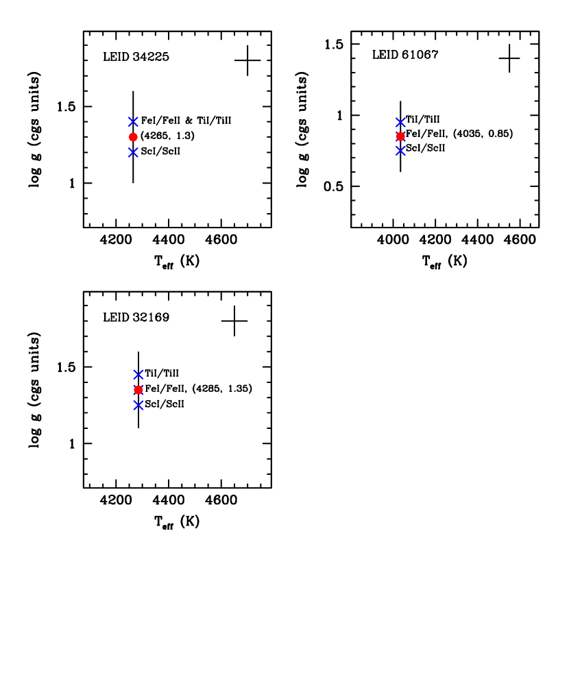
Figure 3: Figure shows the plane of $T_{\rm eff}$ and log g for LEID 34225, LEID 61067, LEID 32169. The verticle line shows the excitation balance from Fe i lines. The blue crosses on the verticle line are the log $g$ values derived from the ionization balance of Fe i/Fe ii, Sc i/Sc ii and Ti i/Ti ii. The mean/adopted ($T_{\rm eff}$, log $g$) is shown with a red dot. The error bars on the $T_{\rm eff}$ and log g are shown in the top right corner. See figure for the keys.

For abundance analyses, the linelist of Johnson & Pilachowski (2010) was used. The elements for which the lines are very few or none in Johnson & Pilachowski (2010) list, were adopted from Ramírez & Allende Prieto (2011). However, to cross examine, the stellar parameters and the Fe abundances were also derived from the Fe i and Fe ii lines of Ramírez & Allende Prieto (2011) for one of the program stars i.e. LEID 34225. These parameters derived are in line with those determined from the Fe i and Fe ii lines of Johnson & Pilachowski (2010). The linelist used for the determination of the stellar parameters and the abundances for the program stars are given in Table 2. The Fe i and Fe ii lines of Ramírez & Allende Prieto (2011) for LEID 34225 are given in Table 3. Table 4 gives the abundance ratios ([E/Fe]) for different elements of the program stars. The adopted solar abundances from Asplund et al. (2009) is also given. The typical errors on elemental abundances due to the uncertainties on the stellar parameters and the signal-to-noise are given in Table 5. The root-mean-square error due to these parameters is given along with the standard deviation in the abundances due to line-to-line scatter, in the last two columns of Table 5. An Mg i line at 5711Å in our program stars is also synthesized to support the Mg abundance derived from Mg i equivalent width analysis (see Figure 4).

Table 4: The derived abundance ratios for the program stars. The adopted solar abundances from Asplund et al. (2009) are also given.

	Sun	39048			61067			34225			32169
Elements	log$\epsilon$(E)	[E/Fe]	n		[E/Fe]	n		[E/Fe]	n		[E/Fe]	n
O i	8.69	0.03	2		0.14	1		-0.05	1		0.11	2
Na i	6.24	0.88	2		1.17	4		0.52	4		0.77	4
Mg i	7.60	0.43	5		0.41	5		0.1	4		0.26	4
Mg from MgH	$\cdots$	0.02	$\cdots$		0.26	$\cdots$		-0.28	$\cdots$		0.25	$\cdots$
Al i	6.45	0.67	4		0.92	4		1.09	4		0.75	4
Si i	7.51	0.47	7		0.64	7		0.53	5		0.38	6
Ca i	6.34	0.18	8		0.32	9		0.11	9		0.31	10
Sc i	3.15	$\cdots$	$\cdots$		0.12	6		0.13	4		0.0	3
Sc ii	$\cdots$	0.06	5		0.14	7		0.14	5		0.1	5
Ti i	4.95	0.48	11		0.46	17		0.39	7		0.1	14
Ti ii	$\cdots$	$\cdots$	$\cdots$		0.46	3		0.39	4		0.1	3
V i	3.93	-0.11	8		0.08	7		-0.23	6		-0.07	8
Cr i	5.64	-0.02	5		0.02	7		0.0	7		0.01	6
Mn i	5.43	0.04	3		-0.02	5		0.01	3		0.02	2
Fe i	7.50	-0.62	16		-1.01	19		-1.05	21		-1.05	16
Fe ii	$\cdots$	$\cdots$	$\cdots$		-1.05	2		-1.05	2		-1.06	2
Co i	4.99	-0.06	7		0.02	8		0.05	6		-0.04	5
Ni i	6.22	0.14	7		-0.01	8		-0.06	3		-0.02	9
La ii	1.10	0.62	1		1.21	1		1.04	1		1.0	1

Note. — ^a First group H-deficient star.

^b Third group H-deficient star.

^c First group normal stars.

^d n is the number of lines used in the analysis.

Table 5: Errors due to the uncertainties on the stellar parameters of LEID 34225, defined by $\Delta$(log $\epsilon_{i}$) = log $\epsilon_{i}$ (perturbed) - log $\epsilon_{i}$ (adopted). The adopted parameters are $T_{\rm eff}$ = 4265K, log $g$ = 1.3 (cgs), and $\xi_{turb}$= 1.6 km s^-1.

Species	$T_{\rm eff}$=$-$50	log $g$=$-$0.1	$\xi_{turb}$=$-$0.1	ErrorS/N	RMS	SD
	[K]	[cgs]	km s-1
O i	-0.04	-0.01	0.03	0.08	0.09	$\cdots$
Na i	-0.06	-0.05	0.01	0.09	0.11	0.16
Mg i	-0.02	-0.005	0.02	0.1	0.10	0.05
Mg(MgH)	$\cdots$	$\cdots$	$\cdots$	0.05	0.05	$\cdots$
Al i	-0.04	0.0	0.025	0.08	0.10	0.12
Si i	0.03	-0.025	0.02	0.09	0.10	0.11
Ca i	-0.08	-0.005	0.04	0.07	0.11	0.16
Sc i	-0.01	-0.04	0.04	0.09	0.10	0.16
Sc ii	-0.01	-0.045	0.02	0.08	0.09	0.09
Ti i	-0.1	-0.005	0.035	0.1	0.13	0.14
Ti ii	0.01	-0.04	0.07	0.08	0.11	0.11
V i	-0.12	-0.01	0.01	0.09	0.14	0.14
Cr i	-0.07	0.0	0.02	0.09	0.11	0.13
Mn i	-0.07	-0.005	0.015	0.1	0.11	0.06
Fe i	-0.04	-0.025	0.045	0.1	0.12	0.16
Fe ii 0.08	-0.055	0.015	0.08	0.13	0.06
Co i	-0.01	-0.025	0.015	0.09	0.10	0.14
Ni i	-0.06	-0.02	0.015	0.1	0.11	0.1
La i	-0.02	-0.06	0.1	0.09	0.14	$\cdots$

^a Root-mean-square of the error on $T_{\rm eff}$, log $g$, $\xi_{t}$ and the error on Signal-to-noise ratio of the spectrum.
^b SD, the standard deviation on the abundance due to the line-to-line scatter.
^c The error on synthesis due to the error in signal-to-noise is given. Errors due to uncertainties on the stellar parameters for MgH band is discussed in Table 6.

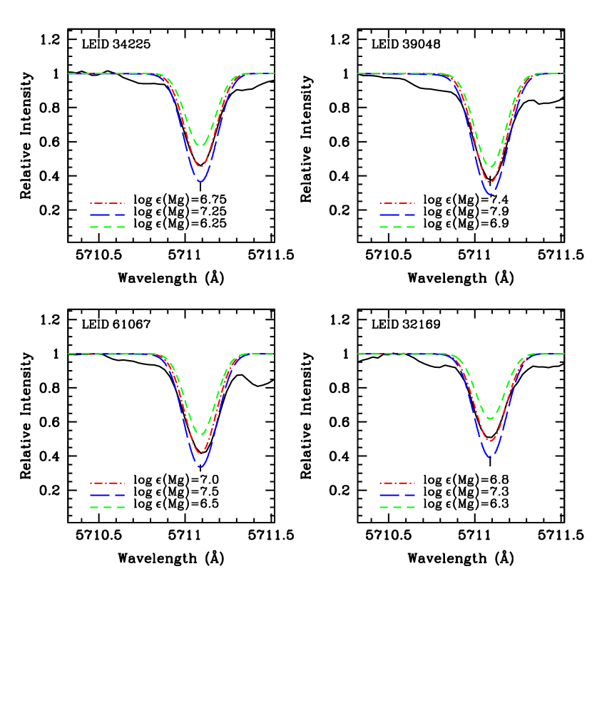
Figure 4: Figure show the synthesis of Mg i line at 5711Å for the program stars. The synthesis is shown for the best fit Mg abundance and also for other two Mg abundances for comparison. See figure for the keys.

Table 6: The derived Mg abundances from Mg i lines and the MgH band for the adopted and for the uncertainties on the stellar parameters. The adopted stellar parameters and their corresponding derived Mg abundances are given in boldface.

Stars	$T_{\rm eff}$	log $g$	[Mg/Fe] from Mg i	[Mg/Fe] from MgH
LEID 39048	3965	0.95	$+$0.42	$+$0.02
	4015	0.95	$+$0.41	$+$0.11
	3915	0.95	$+$0.44	$-$0.06
	3965	1.05	$+$0.44	$-$0.08
	3965	0.85	$+$0.42	$+$0.02
LEID 34225	4265	1.30	$+$0.10	$-$0.30
	4315	1.30	$+$0.10	$-$0.25
	4215	1.30	$+$0.06	$-$0.44
	4265	1.40	$+$0.04	$-$0.26
	4265	1.20	$+$0.06	$-$0.26

4 MgH band and the Spectrum syntheses

In our previous study (Hema & Pandey, 2014), the low-resolution optical spectra of the globular cluster $\omega$ Cen giants were analysed to identify the H-deficient stars by examining the strengths of the Mg $b$ atomic lines and the blue degraded (0,0) MgH band. Based on the strengths of these features, the observed program stars were devided into three groups, first: metal rich giants with strong Mg $b$ lines and also the MgH band; second: metal poor giants with no Mg $b$ line and no MgH band; third: metal rich giants with strong Mg $b$ lines and weak/no MgH band, in their observed spectra. Hema & Pandey (2014)’s analysis, that included comparison of stars’ spectra with similar stellar parameters and spectrum synthesis of the MgH band for the star’s adopted stellar parameters, resulted in identification of four mildly H-deficient stars: two from the first group (LEID 39048 and LEID 60073) and two from the third group (LEID 34225 and LEID 193804).

High resolution spectra of two stars, LEID 39048 – a first group star, and LEID 34225 – a third group star, including two comparison stars were obtained from SALT for confirming their H-deficiency. For example, SALT spectrum of LEID 34225 is superposed on the SALT spectrum of a comparison star, LEID 32169 (see Figure 5), note that both these stars have similar stellar parameters i.e. effective temperature, surface gravity, and metallicity. As discussed in Hema & Pandey (2014), the strengths of MgH bands in the observed spectra of LEID 39048 and LEID 34225 are weaker than that expected for their derived stellar parameters. To validate our continuum fitting in the MgH band region, we measured the equivalent width for the Fe i lines in this region and derived the abundances. The derived abundances are in excellent agreement with those derived from the other wavelength regions.

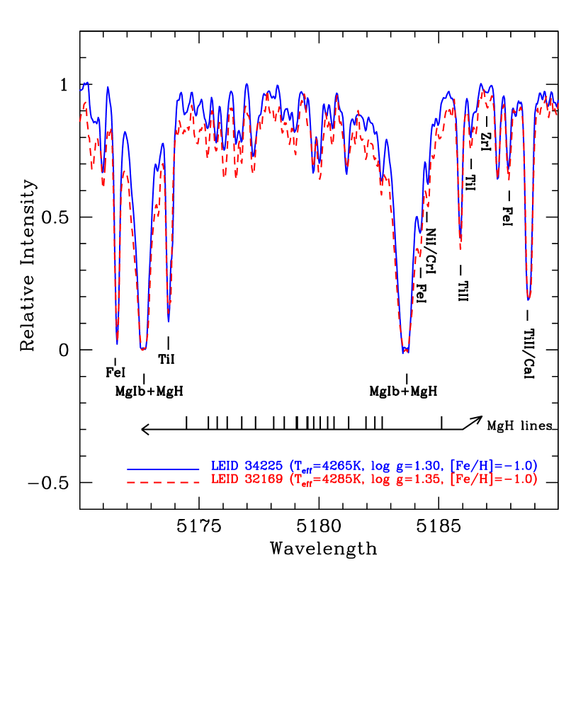
Figure 5: Figure shows the strengths of (0,0) MgH band in the spectra of first group stars: LEID 34225 (sample) and LEID 32169 (comparison). The key lines are marked.

For their derived stellar parameters, the spectra of these stars were synthesized in the window 5170Å to 5190Å to examine the strengths of Mg $b$ lines and the MgH bands in their observed spectra carefully. The spectrum synthesis for the program stars were carried out following the procedure explained in Hema & Pandey (2014). Using the LTE spectrum synthesis code $synth$ in MOOG, combined with ATLAS9 (Kurucz, 1998) plane parallel, line-blanketed LTE model atmospheres, and the molecular and the atomic line lists both, validated by synthesizing the high-resolution spectrum of Arcturus provided by Hinkle et al. (2000), were used to synthesize the spectra of our program stars. The Mg isotopic ratio, ²⁴Mg:²⁵Mg:²⁶Mg; 82:09:09 was adopted for Arcturus from McWilliam & Lambert (1988). The synthesized spectrum was convolved with a Gaussian profile with a width that represents the instrumental broadening, as the effects due to macroturbulence and the rotational velocity are very small or negligible.

The spectra were synthesized in the wavelength window from 5170 to 5190Å. The observed spectrum bluer to 5170Å falls at the edge of the order. Our examination of the observed spectra show very strong saturated Mg $b$ lines at 5167.3Å  5172.68Å  and 5183.6Å; The subordinate lines of MgH band are blended with these strong Mg $b$ lines. Hence, the subordinate lines between the wavelength region 5175Å and 5176Å  where there are pure molecular lines, were given more weight. However, a fit to these MgH features gives an overall best fit to the whole range of MgH band spanning from about 5160Å to 5190Å. The mean of the isotopic ratios derived for red giants $\omega$ Cen by Da Costa et al. (2013), which is about ²⁴Mg:²⁵Mg:²⁶Mg;70:13:15 with the uncertainty on each value of about $\pm$4, was adopted for our program stars that provides a fairly good fit through out the span of the MgH band. Note that, the Mg $b$ lines are very strong and are saturated in the spectra of our program stars, hence, these lines are not used for estimating the Mg abundance from Mg i line or MgH band. The weaker atomic Mg i lines are used for deriving the Mg i abundance (those given in Table 2) and the Mg abundance from MgH band is derived using pure MgH molecular lines which are not blended with the strong Mg $b$ lines.

The spectra of the program stars, were synthesized using their derived stellar parameters and the elemental abundances as discussed in section 3. The syntheses of the spectra for the individual program stars are discussed below.

LEID 32169: this is a first group star, which is relatively metal rich having strong Mg $b$ lines and a strong MgH band. This is a comparison for the first group mildly H-deficient stars and here for the sample star, LEID 34225. The spectrum of LEID 32169 shows a well represented MgH band. Using its derived stellar parameters: ($T_{\rm eff}$, log $g$, $\xi_{t}$, [Fe/H]): (4285$\pm$50, 1.35$\pm$0.1, 1.6$\pm$0.1, -1.0), the MgH band is synthesized by varying the Mg abundance to obtain the best fit for the observed spectrum (see Figure 6). The MgH band synthesized for the log $\epsilon$(Mg) = 6.8 dex ([Mg/Fe]=$+$0.26) provides the best fit to the observed spectrum, and this is in excellent agreement with the Mg abundance derived from Mg i lines. The Mg abundance derived from the MgH band is as expected for the star’s metallicity and also that derived from the Mg i lines.

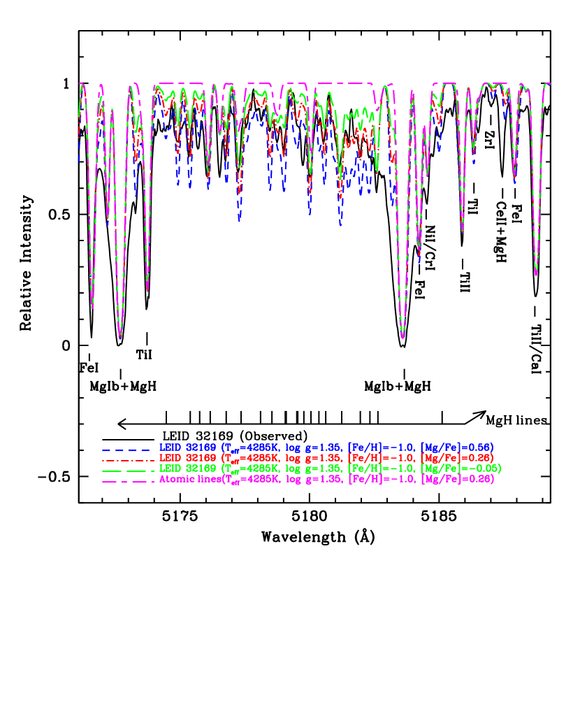
Figure 6: Figure shows the superposition of the observed and the synthesized spectra for the normal sample star LEID 32169. The spectrum is synthesized for the star’s derived stellar parameters and the Mg abundance. The synthesis is shown for the best fit [Mgi/Fe]=$+$0.26 with red dash-dotted line and the syntheses for [Mg/Fe]=$+$0.56 is shown with blue short-dashed line, and for the [Mg/Fe]=$-$0.05 is shown with green long-dashed line, for comparison. The synthesis for pure atomic lines is also shown with magenta short-long dashed line. The key lines are marked.

LEID 61067: This is a first group star, which is relatively metal rich having strong Mg $b$ lines and a strong MgH band. This is a comparison for the third group sample star LEID 39048. The observed spectrum shows the well represented MgH band for its derived stellar parameters: ($T_{\rm eff}$, log $g$, $\xi_{t}$, [Fe/H]): (4035$\pm$50 K, 0.85$\pm$0.1, 1.6$\pm$0.2, -1.0). The MgH band is synthesized by varying the Mg abundance. The spectrum synthesized for log $\epsilon$(Mg) = 6.85 dex ([Mg/Fe]=$+$0.25) provides the best fit to the observed spectrum (see Figure 7). The derived Mg abundance from Mg i lines is about 7.0$\pm$0.1 ([Mg/Fe] = $+$0.4). The Mg abundance required for obtaining the best fit for the observed spectrum is 6.85 dex and this is about 0.15 dex less than that derived from Mg i lines, but are in fair agreement within the uncertainties on the derived abundances.

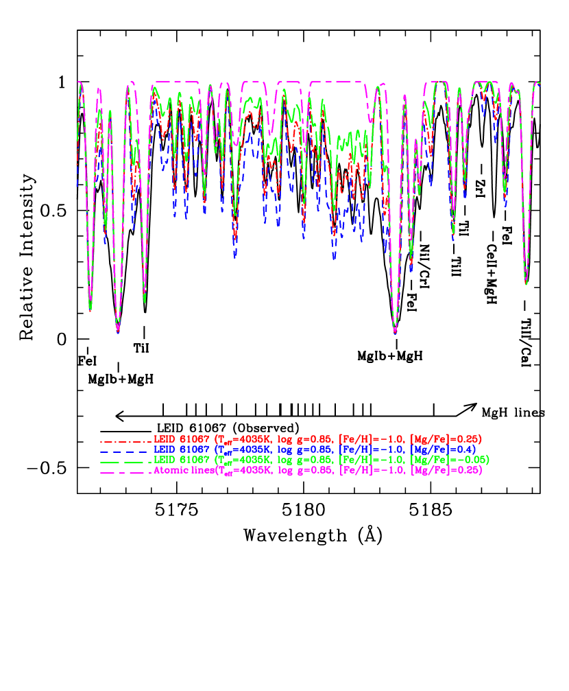
Figure 7: Figure shows the superposition of the observed and the synthesized spectra for the sample star LEID 61067. The spectrum is synthesized for the star’s derived stellar parameters and the Mg abundance. The synthesis is shown for [Mg/Fe]=$+$0.4 with blue short-dashed line, the best fit [Mg/Fe]=$+$0.25 with red dash-dotted line, and also for [Mg/Fe]=$-$0.05 with green long-dashed line for comparison. Note that the Mg abundance obtained from Mg i and MgH are in fair agreement within the errors. The synthesis for pure atomic lines is also shown with magenta short-long dashed line. The key lines are marked.

LEID 39048: This is the first group sample star, which is relatively metal rich having strong Mg $b$ lines and the MgH band. From the previous study, that is the low resolution spectroscopic studies of $\omega$ Cen giants (Hema & Pandey, 2014), this is one of the identified mildly H-deficient stars of our sample, having a very low Mg abundance as expected for its metallicity as well as from the mean Mg abundance of the $\omega$ Cen giants. The Mg abundance was estimated from the MgH band for the star’s derived stellar parameters.

In the present study we have used a high-resolution spectrum. The MgH band is synthesized for the star’s derived stellar parameters: ($T_{\rm eff}$, log $g$, $\xi_{t}$, [Fe/H]): (3965$\pm$50 K, 0.95$\pm$0.1, 1.6$\pm$0.2, -0.65), and for the Mg abundance determined from Mg i lines of 7.4 dex ([Mg/Fe]=$+$0.42). To obtain the best fit for the MgH band the Mg abundance has to be reduced by about 0.4 dex than that determined from Mg i lines. This best fit value of the Mg abundance, derived from the MgH band, is beyond the uncertainty limit on the derived Mg abundance from Mg i lines. Hence, this confirms our 2014 results using a low resolution spectrum. Figure 8 shows the synthesis for LEID 39048 for the best fit Mg abundance and also for the derived Mg abundance from Mg i lines, including a different Mg abundance, which do not provide the best fit to the observed MgH band.

Spectrum of the program stars LEID 39048 in the MgH band region was synthesized by changing the stellar parameters within the uncertainties that are discussed in section 3. Our aim was to explore whether the difference in Mg abundance, from Mg i lines and from MgH band, could be accounted by making changes in the adopted stellar parameters within the uncertainties. The synthesized MgH band for the uncertainties on effective temperature that are $+$50K and $-$50K, provides the best fit for the Mg abundance which is about 0.3 dex and 0.5 dex lower than the Mg abundance from Mg i lines, respectively (see Table 6). Similarly, the MgH band is also synthesized for the uncertainties on the log $g$ value that are $\pm$0.1. For the log $g$ values $-$0.1 and $+$0.1 of the adopted log $g$, the synthesized MgH band provides the best fit for the Mg abundance which is about 0.4 and 0.5 dex lower than that derived from the Mg i lines, respectively (see Table 6).

Similar excercise was done with the uncertainties on the microturbulence; the strength of the synthesized MgH band show no appreciable difference with the change in microturbulence.

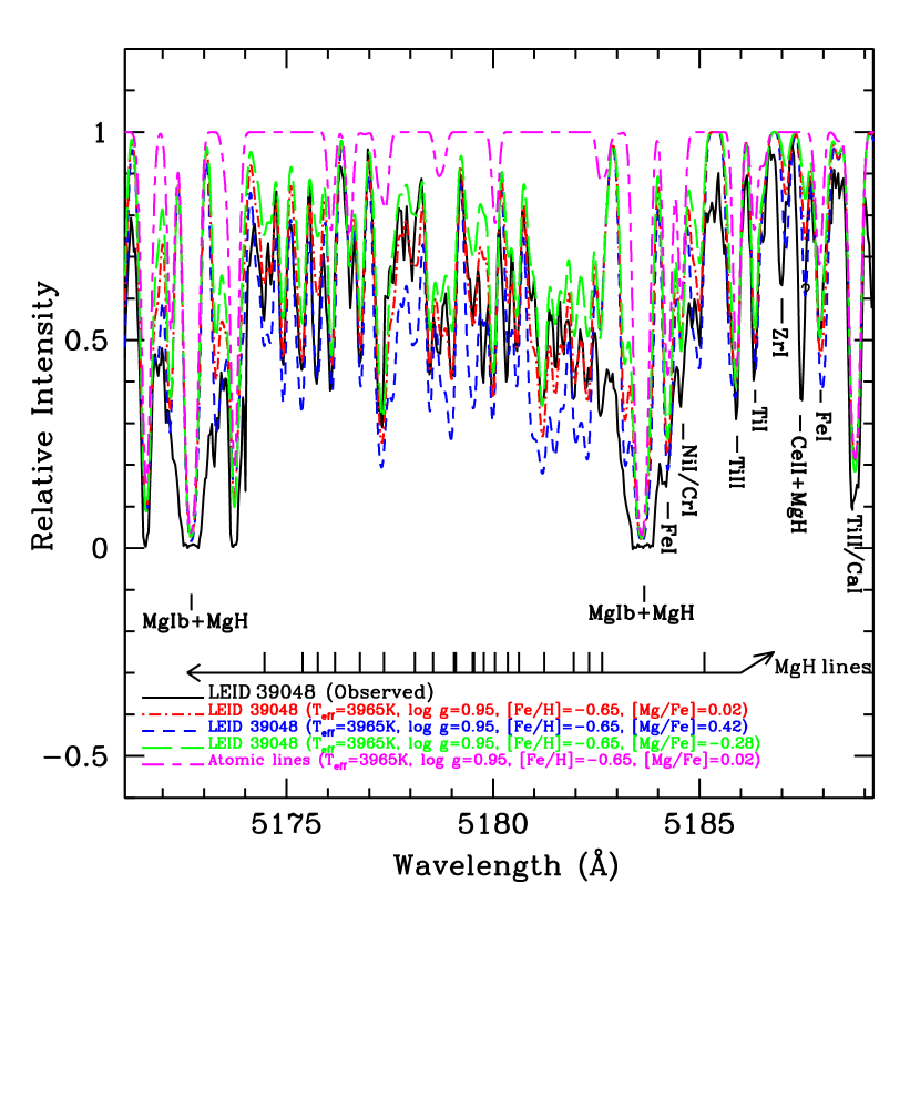
Figure 8: Figure shows the superposition of the observed and the synthesized spectra for the sample star LEID 39048. The spectrum is synthesized for the star’s derived stellar parameters and the Mg abundance. The synthesis is shown for [Mg/Fe]=$+$0.42 from Mg i lines with blue short-dashed line, the best fit [Mg/Fe]=$+$0.02 with red dash-dotted line, and also for [Mg/Fe]=$-$0.28 with green long-dashed line, for comparison. The synthesis for pure atomic lines. is also shown with magenta short-long dashed line. The key lines are marked.

LEID 34225: This is a third group sample star which is relatively metal rich having strong Mg $b$ lines and the MgH band. From our previous study (Hema & Pandey, 2014), that is the low resolution spectroscopic studies of $\omega$ Cen giants, this is one of the mildly H-deficient stars of our sample giving a very low Mg abundance than expected for its metallicity and also from the mean Mg abundance of the $\omega$ Cen giants. This low Mg abundance was derived by synthesizing the MgH band for the star’s adopted stellar parameters using the observed low resolution spectrum.

A high-resolution spectrum is used in the present study. The MgH band is synthesized for the star’s derived stellar parameters: ($T_{\rm eff}$, log $g$, $\xi_{t}$, [Fe/H]): (4265$\pm$50 K, 1.30$\pm$0.1, 1.6$\pm$0.1, -1.0) and for the Mg abundance determined from Mg i lines of 6.65$\pm$0.05 dex ([Mg/Fe]=0.1). To obtain the best fit to the observed high-resolution spectrum, the Mg abundance has to be reduced by about 0.4 dex than that derived from Mg i lines. This best fit value of the Mg abundance is outside the uncertainty limits on the Mg abundance from Mg i lines. Hence, this confirms our 2014 results. Figure 9 shows the synthesis of the MgH band for the best fit Mg abundance, for the derived Mg abundance from Mg i lines, and also for a lower Mg abundance than that provided the best fit.

The spectra of the MgH band region were synthesized by changing the stellar parameters within the uncertainties that are discussed in section 3. Our aim was to explore whether the difference in Mg abundance, from Mg i lines and from MgH band, could be accounted by making changes in the adopted stellar parameters within the uncertainties. The synthesized MgH band for the uncertainties on effective temperature that are $+$50K and $-$50K, provides the best fit for the Mg abundance which is about 0.3 dex and 0.5 dex lower than the Mg abundance from Mg i lines, respectively (see Table 6). Similarly, the MgH band is also synthesized for the uncertainty on the log $g$ value that are $\pm$0.1. For the log $g$ values, $-$0.1 and $+$0.1 of the adopted log $g$, the synthesized MgH band provides the best fit for the Mg abundance which is about 0.3 dex lower than that derived from the Mg i lines, respectively (see Table 6).

Similar excercise was done with the uncertainties on the microturbulence; The strength of the synthesized MgH band show no appreciable difference with the change in microturbulence.

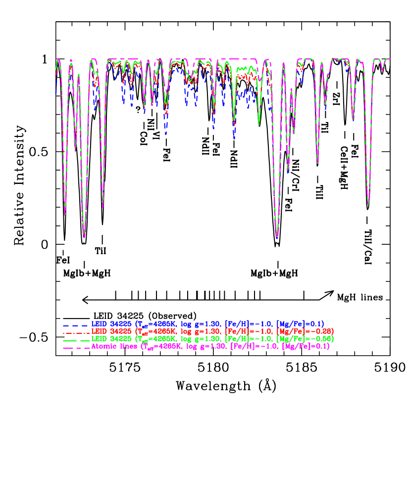
Figure 9: Figure shows the superposition of the observed and the synthesized spectra for the sample star LEID 34225. The spectrum is synthesized for the star’s derived stellar parameters and the Mg abundance. The synthesis is shown for [Mg/Fe] = $+$0.1 from Mg i lines with blue short-dashed line, the best fit [Mg/Fe] of $-$0.28 with the red dash-dotted line, and also for [Mg/Fe] of $-$0.56 with green long-dashed line for comparison. The synthesis for pure atomic lines is also shown with magenta short-long dashed line. The key lines are marked.

5 Discussion

The aim of Hema & Pandey (2014) was to identify the H-deficient stars of RCB type, which show a severe H-deficiency. The features that directly indicate the H-deficiency are H-Balmer lines, CH-band, etc. H$\beta$ and CH-band were not covered in the observed low-resolution spectra, however, saturated H$\alpha$ line is present. Hence, the (0,0) MgH band was used for the analysis. The region of (0,0) MgH band also includes the strong Mg $b$ lines, and these indicate the appropriate metallicity and the Mg abundance of the program stars. The four stars that were identified as H-poor, were confirmed by the spectrum synthesis. Though the accurate stellar parameters and the metallicity were available for the program stars, the Mg abundances were not known. In this study, the stellar parameters and the elemental abundances, especially the Mg abundance from Mg i lines, were rederived using the high-resolution spectra of the program stars obtained from SALT-HRS.

In the observed high-resolution spectra, initially we looked for the strengths of the H-Balmer line and the CH-band. But the H-Balmer lines in the observed spectra of the program stars are strong and as expected for the stars’ stellar parameters. The CH-band couldn’t be detected in the spectra of these stars, due to poor signal at about 4300Å. Hence, the analyses is based on the strength of the (0,0) MgH band in the observed SALT spectra. The two stars are mildly H-poor as expected. According to Hema & Pandey (2014), the third group sample star LEID 34225 has strong Mg $b$ lines and weak/no MgH band. The same traits are observed in the high-resolution spectrum of this star. And, the first group sample star LEID 39048 having strong Mg $b$ lines and strong MgH band, is also in line with its SALT high-resolution spectrum. The observed MgH band of the program stars was analysed mainly by spectrum synthesis.

For LEID 32169, a normal (H-rich) comparison star, the best fit of the synthesized spectrum of the MgH band, for the star’s adopted stellar parameters, to the observed spectrum is obtained for the Mg abundance of 6.8 dex (see Figure 6). The Mg abundance derived from the Mg i lines and the MgH band are in excellent agreement, as expected. Similarly, for LEID 61067, a normal (H-rich) comparison star, the best fit of the synthesized spectrum of the MgH band, for the star’s adopted stellar parameters, to the observed spectrum is obtained for the Mg abundance of 6.85 (see Figure 7). This Mg abundance from MgH band is about 0.15 dex less than the derived Mg abundance from the Mg i lines. This difference in abundance is within the uncertainties, which is about $\pm$0.1 dex on the derived Mg abundance from Mg i lines.

For LEID 39048, a candidate H-deficient star of our sample, the best fit of the synthesized spectrum of the MgH band, for the star’s adopted stellar parameters, to the observed spectrum is obtained for the Mg abundance of 7.0 dex ([Mg/Fe]=0.02 dex) (see Figure 8). This Mg abundance is about 0.4 dex less than that derived from the Mg i lines. This difference between the derived Mg abundance from Mg i lines and that from MgH band is greater than the uncertainty on the Mg abundances from Mg i lines. The spectra were also synthesized by changing the stellar parameters within the uncertainties, the derived Mg abundance from Mg i lines and that from the MgH band do not match even within the uncertainties. The Mg abundance required to fit the observed spectrum for the adopted stellar parameters and the uncertainties on them, always require the Mg abundance that is lower by about or more than 0.3 dex than that derived from the Mg i lines (see Table 6). This difference between the Mg abundance from Mg i lines and the MgH band is not acceptable, as the Mg abundance from Mg i lines and that from the MgH band are expected to be same within the uncertainties (as seen from the analysis of the spectra of the normal comparison stars – see above).

Similarly, for LEID 34225, another candidate H-deficient star of our sample, the best fit of the synthesized spectrum, for the star’s adopted stellar parameters, to the observed spectrum is obtained for the Mg abundance of 6.28 dex ([Mg/Fe]=$-$0.3) (see Figure 9). This Mg abundance is about 0.4 dex less than that derived from the Mg i lines. The spectra were also synthesized by changing the stellar parameters within the uncertainties. The Mg abundance required to fit the observed spectrum for the adopted stellar parameters and the uncertainties on them, always require the Mg abundance that is lower by about or more than 0.3 dex than that derived from the Mg i lines (see Table 6). This difference between the Mg abundance from Mg i lines and the MgH band is not acceptable, as the Mg abundance from Mg i lines and that from the MgH band are expected to be same within the uncertainties.

The galactic globular cluster $\omega$ Cen is well known for hosting multiple stellar populations not only in the red giant branch stars, but also in the main-sequence, and sub giant branches. Among the red giant stars, about four distinct subpopulations are identified by Calamida et al. (2009), viz. metal-poor; ([Fe/H] $\leq$ $-$1.49), metal-intermediate; ($-$1.49 $<$ [Fe/H] $\leq$ $-$0.93), metal-rich; ($-$0.95 $<$ [Fe/H] $\leq$ $-$0.15), and solar metallicity; ([Fe/H] $\approx$ 0). Among the subgiant branch stars, there are about three distinct subpopulations identified by Villanova et al. (2007), viz. SGB-metal poor; ([Fe/H] $\sim$ $-$1.7), SGB-Metal-intermediate; ($-$1.7 $<$ [Fe/H] $<$ $-$1.4), and SGB-a; ([Fe/H] $\sim$ $-$1.1). Based on the metallcity, two main-sequences (MS) are identified by Piotto et al. (2005), viz. a red MS with ([Fe/H] $\sim$ $-$1.6), and a blue MS with ([Fe/H] $\sim$ $-$1.3). There are also multiple stellar population studies in horizontal branch (HB) stars by Tailo et al. (2016). They identify the HB stars as, metal-poor; ($-$2.25 $\leq$ [Fe/H] $\leq$ $-$1.4), metal-intermediate; ($-$1.4 $\leq$ [Fe/H] $\leq$ $-$1.1), and metal-rich; ([Fe/H] $\geq$ $-$1.1).

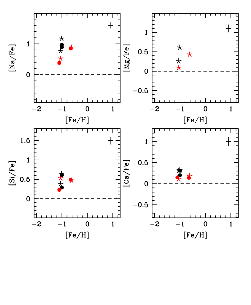
Figure 10: The abundance ratios with respect to solar versus metallicity for the program stars are shown. The red stars are the mildly H-deficient stars and the black stars are the normal comparison stars. The filled circles represents the elemental abundances derived by Johnson & Pilachowski (2010) for the program stars, the red circles the mildly H-deficient/He-enhanced stars and black circles the normal (H-rich) stars. The horizontal dotted lines shows the solar scaled abundance values. The error bars on the abundance ratios are shown with crossed thicklines in the top right corner.

According to these subpopulations, from the main-sequence, through SGB, RGB, there is a metal rich group having the metallicity ([Fe/H] $\sim$ $-$1.1$\pm$0.3), derived spectroscopically, which suggests that they are closely related. From the detailed studies of the main-sequence branches, it is revealed that, the bMS stars are helium enriched with an amount (0.35 $<$ Y $<$ 0.45) and are metal rich by about 0.3 dex than the majority red main-sequence stars which are He-normal (Y = 0.28). However, there are no helium enchancement studies reported for SGB stars, but the SGBs with metallicities similar to the bMS stars are observed. And, these are identified as SGB-a group by Villanova et al. (2007). Villanova et al. (2007) have compared their results of the abundance analyses of SGB-a stars with that of the bMS stars from Piotto et al. (2005). The drived abundances, [C/Fe], [N/Fe], and [Ba/Fe], for bMS stars and SGB-a are very similar, ascertaining the connection between these groups. Pancino et al. (2011) has studied metal rich subgiants for determining their lithium abundance along with the $\alpha$-peak elements, [Al/Fe] and [Ba/Fe]. These abundance ratios: [$\alpha$/Fe], [Al/Fe] and [Ba/Fe] for their sample are in agreement with the literature. They suspect that, all the H-burning processes, where He is produced, happens at temperatures where Li is destroyed. Therefore, He-rich stars should have a very low lithium content. In their sample, they have found a lithium abundance which is lower than that expected for these metal-rich subgiants (see Pancino et al. (2011)for details). Hence, it is an indirect clue that, the metal-rich subgiant stars are He-rich.

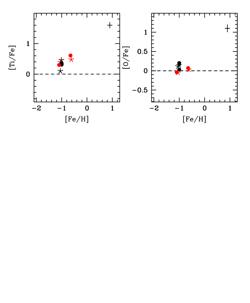
Figure 11: The abundance ratios with respect to solar versus metallicity for the program stars are shown. The red stars are the mildly H-deficient stars and the black stars are the normal comparison stars. The filled circles represents the elemental abundances derived by Johnson & Pilachowski (2010) for the program stars, the red circles the mildly H-deficient/He-enhanced stars and black circles the normal (H-rich) stars. The horizontal dotted lines shows the solar scaled abundance values. The error bars on the abundance ratios are shown with crossed thicklines in the top right corner.

In connection to evolution of the metal rich stars, our program stars provide further link to this evolutionary track. Our program stars are metal rich with the metallicity ([Fe/H] $\geq$ $-$1.1). Using the high-resolution spectra, a detailed abundance analyses is carried out. In order to check the similarities of our program stars with the metal rich stars of MS;bMS, and SGB;SGB-a, we compared their elemental abundances. Mainly the $\alpha$- and the Fe-peak elements are compared as these remain unaltered in the course of the evolution of these stars. The elemental abundances determined for the program stars agree within $\pm$0.2 dex with those derived by Johnson & Pilachowski (2010). This uncertainty arises as the spectra used are obtained from different instruments with different resolution. The solar-scaled elemental abundances plotted vs. metallicity for the program stars are shown in Figure 10, 11 and 12. The abundance ratios from Johnson & Pilachowski (2010) are shown with filled circles. Johnson & Pilachowski (2010) have adopted the solar abundances from Anders & Grevesse (1989) and we have adopted the solar abundances from Asplund et al. (2009); differences due to the adopted solar abundances are taken into account. The $\alpha$ processed elements, such as Mg, Si and Ca show enhacement by about 0.2 to 0.7 dex which is in fair agreement with those derived by Johnson & Pilachowski (2010) for the metal-rich RGB stars of $\omega$ Cen (see Figure 10). [Na/Fe] shows enhancement of about 0.5-1.2 dex for the program stars, which is as expected for the metal rich stars from Johnson & Pilachowski (2010) (see Figure 10). [Ti/Fe] shows an enhancement on an average of 0.35 dex for the program stars (see Figure 11). Johnson & Pilachowski (2010) finds that for the metal rich RGBs [Ti/Fe] $\approx$ 0.3 dex. The Fe-peak elements such as, Cr, Mn, Co, and Ni do not show any enhancement (see Figure 12). Johnson & Pilachowski (2010) has given the abundances of Ni for the RGBs which is in good agreement with that of our program stars.

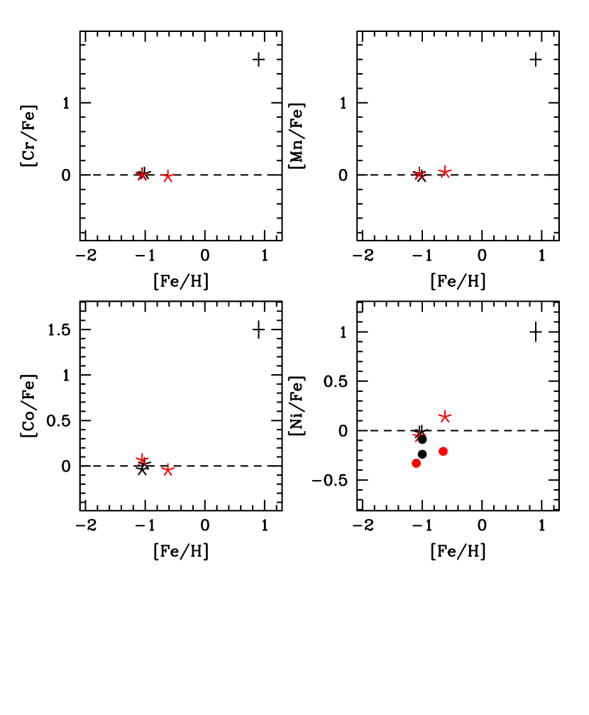
Figure 12: The abundance ratios with respect to solar versus metallicity for the program stars are shown. The red stars are the mildly H-deficient stars and the black stars are the normal comparison stars. The filled circles represents the elemental abundances derived by Johnson & Pilachowski (2010) for the program stars, the red circles the mildly H-deficient/He-enhanced stars and black circles the normal (H-rich) stars. The horizontal dotted lines shows the solar scaled abundance values. The error bars on the abundance ratios are shown with crossed thicklines in the top right corner.

However, [O/Fe] for our program stars are similar to solar, and do not show any depletion/enhancement, and are also similar to [O/Fe] $\approx$ $-$0.15 (see figure 11) for metal-rich RGBs derived by Johnson & Pilachowski (2010). Marino et al. (2011) has conducted a high-resolution spectroscopic studies for red giant stars of $\omega$ Cen for deriving Fe, Na, O and n-capture elements. They have studied the Na-O anticorrelation for the giants of different metallicity. The giants in the metal-rich regime do not show any Na-O anti-correlation unlike metal-poor and metal-intermediate giants. This is also observed in our program stars. Lanthanum abundance derived for our program stars is from a single line and are in line with the [La/Fe] vs. [Fe/H] plots given by Johnson & Pilachowski (2010); Marino et al. (2011, 2012); D’Orazi et al. (2011).

For the SGB-a stars, Villanova et al. (2007) has derived the abundances for Ca and for Ti along with C, N and Ba. The enhancements, [Ca/Fe] and [Ti/Fe] of 0.48 dex and 0.44 dex, respectively, for SGB-a stars by Villanova et al. (2007), are in good agreement with the enhancements, [Ca/Fe] and [Ti/Fe] of 0.35 dex and 0.3 dex, respectively, for our program stars. Similarly, Pancino et al. (2011) have determined the [$\alpha$/Fe] =$+$0.4 dex, [Al/Fe] = $+$0.32 dex, [Fe-peak/Fe] $\sim$ 0.0 dex which are in excellent agreement with those determined by Villanova et al. (2007) and also those determined for metal-rich giants by Johnson & Pilachowski (2010) and in this study. These abundance similarities links the SGB-a stars with the metal rich RGB stars of $\omega$ Cen.

A very important link between: bMS, SGB-a, metal-rich RGBs, come from the helium enhancement. An unacceptable lower Mg abundance derived for our sample stars, LEID 39048 and LEID 34225, from the MgH bands, (the weaker MgH bands), than that expected for their derived stellar parameters, and the Mg abundances from Mg i lines and the uncertainties on these parameters, suggests the lower hydrogen/He-enhancement in their atmospheres.

Hence, similar to bMS stars, our sample stars which are metal rich RGBs, show mild deficiency in hydrogen or enhanced helium. All metal rich RGBs may not be H-poor/He-enhanced, but a sub-group of them are. Dupree et al. (2011) have reported the first direct evidence for an enhancement of helium in the metal-poor RGBs of $\omega$ Cen by analyzing the near-infrared He i 10830Å transition in about 12 red giants. From their studies they notice that the He-enhanced giants show enhanced [Al/Fe] and [Na/Fe], than the He-normal giants (see their Figure 10). Figure 13 shows the plot [Al/Fe] vs. [Na/Fe] for our program stars along with Dupree et al. (2011)’s sample stars. Our program stars follow the similar trend as that of Dupree et al. (2011)’s sample stars.

Figure 13: The abundance ratios of [Al/Fe] vs. [Na/Fe] are shown. The open and filled circles are He-normal and He-enhanced giants, respectively from Dupree et al. (2011) and the open and filled triangles are the He-normal and He-enhanced giants, respectively, from this work (TW).

A detailed spectroscopic studies are not available for horizontal branch stars. However, the helium enhancement in horizontal branch stars may also be due to helium-flash or any other processes, and may not be wholly intrinsic (Moehler et al., 2002).

6 Conclusions

This study based on the evaluation of the strengths of the MgH bands in the observed high-resolution spectra and for the stars’ adopted stellar parameters, confirms that LEID 39048 and LEID 34225 are mildly H-deficient/He-enhanced. Discovery and the detailed abundance analysis of these stars provides a direct evidence for the presence of He-enhanced metal rich giants in $\omega$ Cen. These stars provides crucial link to the evolution of the metal rich sub-population of MS, sub giant and red giants.

References

- Alonso et al. (1999) Alonso, A., Arribas, S., & Martínez-Roger, C. 1999, A&AS, 140, 261
- Anders & Grevesse (1989) Anders, E., & Grevesse, N. 1989, Geochim. Cosmochim. Acta, 53, 197
- Asplund et al. (2009) Asplund, M., Grevesse, N., Sauval, A. J., & Scott, P. 2009, ARA&A, 47, 481
- Calamida et al. (2009) Calamida, A., et al. 2009, ApJ, 706, 1277
- Da Costa et al. (2013) Da Costa, G. S., Norris, J. E., & Yong, D. 2013, ApJ, 769, 8
- D’Orazi et al. (2011) D’Orazi, V., Gratton, R. G., Pancino, E., Bragaglia, A., Carretta, E., Lucatello, S., & Sneden, C. 2011, A&A, 534, A29
- Dupree & Avrett (2013) Dupree, A. K., & Avrett, E. H. 2013, ApJ, 773, L28
- Dupree et al. (2011) Dupree, A. K., Strader, J., & Smith, G. H. 2011, ApJ, 728, 155
- Hema & Pandey (2014) Hema, B. P., & Pandey, G. 2014, ApJ, 792, L28
- Hinkle et al. (2000) Hinkle, K., Wallace, L., Valenti, J., & Harmer, D. 2000, Visible and Near Infrared Atlas of the Arcturus Spectrum 3727-9300 A
- Johnson & Pilachowski (2010) Johnson, C. I., & Pilachowski, C. A. 2010, ApJ, 722, 1373
- Kurucz (1998) Kurucz, R. L. 1998, http://kurucz.harvard.edu/
- Marino et al. (2011) Marino, A. F., et al. 2011, ApJ, 731, 64
- Marino et al. (2012) —. 2012, ApJ, 746, 14
- Mayor et al. (1997) Mayor, M., et al. 1997, AJ, 114, 1087
- McWilliam & Lambert (1988) McWilliam, A., & Lambert, D. L. 1988, MNRAS, 230, 573
- Moehler et al. (2002) Moehler, S., Sweigart, A. V., Landsman, W. B., & Dreizler, S. 2002, A&A, 395, 37
- Pancino et al. (2011) Pancino, E., Mucciarelli, A., Bonifacio, P., Monaco, L., & Sbordone, L. 2011, A&A, 534, A53
- Pandey et al. (2004) Pandey, G., Lambert, D. L., Rao, N. K., Gustafsson, B., Ryde, N., & Yong, D. 2004, MNRAS, 353, 143
- Piotto et al. (2005) Piotto, G., et al. 2005, ApJ, 621, 777
- Ramírez & Allende Prieto (2011) Ramírez, I., & Allende Prieto, C. 2011, ApJ, 743, 135
- Simpson & Cottrell (2013) Simpson, J. D., & Cottrell, P. L. 2013, MNRAS, 433, 1892
- Sneden (1973) Sneden, C. A. 1973, PhD thesis, THE UNIVERSITY OF TEXAS AT AUSTIN.
- Sollima et al. (2005) Sollima, A., Ferraro, F. R., Pancino, E., & Bellazzini, M. 2005, MNRAS, 357, 265
- Sumangala Rao et al. (2011) Sumangala Rao, S., Pandey, G., Lambert, D. L., & Giridhar, S. 2011, ApJ, 737, L7
- Tailo et al. (2016) Tailo, M., Di Criscienzo, M., D’Antona, F., Caloi, V., & Ventura, P. 2016, MNRAS, 457, 4525
- Villanova et al. (2007) Villanova, S., et al. 2007, ApJ, 663, 296