The Sparse Variance Contamination Model

Abstract

We consider a Gaussian contamination (i.e., mixture) model where the contamination manifests itself as a change in variance. We study this model in various asymptotic regimes, in parallel with the work of Ingster (1997) and Donoho and Jin (2004), who considered a similar model where the contamination was in the mean instead.

1 Introduction

The detection of rare effects becomes important in settings where a small proportion of a population may be affected by a given treatment, for example. The situation is typically formalized as a contamination model. Although such models have a long history (e.g., in the theory of robust statistics), we adopt the perspective of Ingster [5] and Donoho and Jin [4], who consider such models in asymptotic regimes where the contamination proportion tends to zero at various rates. This line of work has mostly focused on models where the effect is a shift in mean, with some rare exceptions [2, 3]. In this paper, instead, we model the effect as a change in variance.

We consider the following contamination model:

$$(1-\varepsilon)\mathcal{N}(0,1)+\varepsilon\mathcal{N}(0,\sigma^{2}),$$ (1)

where $\varepsilon\in[0,1/2)$ is the contamination proportion and $\sigma>0$ is the standard deviation of the contaminated component. (Note that this is a Gaussian mixture model with two components.) Following [5, 4], we consider the following hypothesis testing problem: based on $X_{1},\dots,X_{n}$ drawn iid from (1), decide

$$\mathcal{H}_{0}:\varepsilon=0\quad\text{versus}\quad\mathcal{H}_{1}:\varepsilon>0,\,\sigma\neq 1.$$ (2)

As usual, we study the behavior of the likelihood ratio test, which is optimal in this simple versus simple hypothesis testing problem. We also study some testing procedures that, unlike the likelihood ratio test, do not require knowledge of the model parameters $(\varepsilon,\sigma)$:

• The chi-squared test rejects for large values of $\big{|}\sum_{i}X_{i}^{2}-n\big{|}$. This is the typical variance test when the sample is known to be zero mean.

• The extremes test rejects for combines the test that rejects for small values of $\min_{i}|X_{i}|$ and the test that rejects for large values of $\max_{i}|X_{i}|$ using Bonferroni’s method.

• The higher criticism test [4] amounts to applying one of the tests proposed by Anderson and Darling [1] for normality. One variant is based on rejecting for large values of

  $$\sup_{x\geq 0}\frac{\sqrt{n}\,|F_{n}(x)-\Psi(x)|}{\sqrt{\Psi(x)(1-\Psi(x))}},$$ (3)

  where $\Psi(x):=2\Phi(x)-1$, where $\Phi$ denotes the standard normal distribution, and $F_{n}(x):=\frac{1}{n}\sum_{i=1}^{n}\mathbb{I}\{|X_{i}|\leq x\}$.

The testing problem (2) was partially addressed by Cai, Jeng, and Jin [3], who consider a contamination model where the effect manifests itself as a shift in mean and a change in variance. However, in their setting the variance is fixed, while we let the variance change with the sample size in an asymptotic analysis that is now standard in this literature.

Our analysis reveals three distinct situations:

1. Near zero ($\sigma\to 0$): In the sparse regime, the higher criticism test is as optimal as the likelihood ratio test, while the chi-squared test is powerless and the extremes test is suboptimal.

2. Near one ($\sigma\to 1$): In the dense regime, the chi-squared test and the higher criticism test are as optimal as the likelihood ratio test, while the extremes test has no power.

3. Away from zero and one: In the sparse regime, the extremes test and the higher criticism test are as optimal as the likelihood ratio test, while the chi-squared test is asymptotically powerless if $\sigma$ is bounded.

In the tradition of Ingster [5], we set

$$\varepsilon=n^{-\beta},\quad\beta\in(0,1)\text{ fixed}.$$ (4)

The setting where $\beta\leq 1/2$ is often called the dense regime while the setting where $\beta>1/2$ is often called the sparse regime. (Note that the setting where $\beta>1$ is uninteresting since in that case there is no contamination with probability tending to 1.)

2 The likelihood ratio test

We start with bounding the performance of the likelihood ratio test. As this is the most powerful test by the Neyman-Pearson Lemma, this bound also applies to any other test. We say that a testing procedure is asymptotically powerless if the sum of its probabilities of Type I and Type II errors (its risk) has limit inferior at least 1 in the large sample asymptote.

2.1 Near zero

Consider the testing problem (2) in the regime where $\sigma=\sigma_{n}\to 0$ as $n\to\infty$. More specifically, we adopt the following parameterization as it brings into focus the first-order asymptotics:

$$\sigma=n^{-\gamma},\quad\gamma>0\text{ fixed}.$$ (5)

Theorem 1.

For the testing problem (2) with parameterization (4) and (5), the likelihood ratio test (and then any other test procedure) is asymptotically powerless when

$$\gamma<2\beta-1.$$ (6)

Proof.

The likelihood ratio is

$$L:=\prod_{i=1}^{n}L_{i},$$ (7)

where $L_{i}$ is the likelihood ratio for observation $X_{i}$, which in this case is

$$L_{i} =\frac{\frac{1-\varepsilon}{\sqrt{2\pi}}\exp(-\frac{1}{2}X_{i}^{2})+\frac{\varepsilon}{\sqrt{2\pi}\sigma}\exp(-\frac{1}{2\sigma^{2}}X_{i}^{2})}{\frac{1}{\sqrt{2\pi}}\exp(-\frac{1}{2}X_{i}^{2})}$$ (8)

$$=1-\varepsilon+\frac{\varepsilon}{\sigma}\exp\bigg{(}\frac{\sigma^{2}-1}{2\sigma^{2}}X_{i}^{2}\bigg{)}$$ (9)

The risk of the likelihood ratio test is equal to

$${\rm risk}(L):=1-\frac{1}{2}\operatorname{\mathbb{E}}_{0}|L-1|.$$ (10)

Our goal is to show that ${\rm risk}(L)=1+o(1)$ under the stated conditions. When $\sigma$ is below and bounded away from $\sqrt{2}$, it turns out that a crude method, the so-called 2nd moment method which relies on the Cauchy-Schwarz Inequality, is enough to lower bound the risk. Indeed, by the Cauchy-Schwarz Inequality,

$${\rm risk}(L)\geq 1-\frac{1}{2}\sqrt{\operatorname{\mathbb{E}}_{0}[L^{2}]-1},$$ (11)

and we are left with the task of finding conditions under which $\operatorname{\mathbb{E}}_{0}[L^{2}]\leq 1+o(1)$.

We have

$$\operatorname{\mathbb{E}}_{0}[L^{2}]=\prod_{i=1}^{n}\operatorname{\mathbb{E}}_{0}[L_{i}^{2}]=(\operatorname{\mathbb{E}}_{0}[L_{1}^{2}])^{n},$$ (12)

where

$$\operatorname{\mathbb{E}}_{0}[L_{1}^{2}] =\operatorname{\mathbb{E}}_{0}\bigg{[}\bigg{(}1-\varepsilon+\frac{\varepsilon}{\sigma}\exp\bigg{(}\frac{\sigma^{2}-1}{2\sigma^{2}}X_{1}^{2}\bigg{)}\bigg{)}^{2}\bigg{]}$$ (13)

$$=1-\varepsilon^{2}+\frac{\varepsilon^{2}}{\sigma^{2}}\operatorname{\mathbb{E}}_{0}\bigg{[}\exp\bigg{(}\frac{\sigma^{2}-1}{\sigma^{2}}X_{1}^{2}\bigg{)}\bigg{]}$$ (14)

$$=1-\varepsilon^{2}+\varepsilon^{2}\big{[}\sigma^{2}(2-\sigma^{2})\big{]}^{-1/2}$$ (15)

$$=1+\varepsilon^{2}\Big{(}\big{[}\sigma^{2}(2-\sigma^{2})\big{]}^{-1/2}-1\Big{)}.$$ (16)

Therefore,

$$\operatorname{\mathbb{E}}_{0}[L^{2}]=\bigg{[}1+\varepsilon^{2}\Big{(}\big{[}\sigma^{2}(2-\sigma^{2})\big{]}^{-1/2}-1\Big{)}\bigg{]}^{n}\leq\exp\bigg{[}n\varepsilon^{2}\Big{(}\big{[}\sigma^{2}(2-\sigma^{2})\big{]}^{-1/2}-1\Big{)}\bigg{]},$$ (17)

so that $\operatorname{\mathbb{E}}_{0}[L^{2}]\leq 1+o(1)$ when

$$n\varepsilon^{2}\Big{(}\big{[}\sigma^{2}(2-\sigma^{2})\big{]}^{-1/2}-1\Big{)}\to 0.$$ (18)

Plugging in the parameterization (4) and (5), we immediately see that this condition is fulfilled when (6) holds, and this concludes the proof. ∎

2.2 Near one

Consider the testing problem (2) in the regime where $\sigma^{2}\to 1$. More specifically, we adopt the following parameterization:

$$|\sigma-1|=n^{-\gamma},\quad\gamma>0\text{ fixed}.$$ (19)

Theorem 2.

For the testing problem (2) with parameterization (4) and (19), the likelihood ratio test (and then any other test procedure) is asymptotically powerless when

$$\gamma>1/2-\beta.$$ (20)

Proof.

Restarting the proof of Theorem 1 at (18), and plugging in the parameterization (4) and (19), we immediately see that $\operatorname{\mathbb{E}}_{0}[L^{2}]\leq 1+o(1)$ when (20) holds. ∎

2.3 Away from zero and one

Consider the testing problem (2) in the regime where $\sigma$ is fixed away from 0 and 1. (Some of the results developed in this section are special cases of results in [3].)

Theorem 3.

For the testing problem (2) with parameterization (4) and $\sigma>0$ is fixed, the likelihood ratio test (and therefore any other test) is asymptotically powerless when $\beta>1/2$ and

$$\sigma<1/\sqrt{1-\beta}.$$ (21)

Proof.

We use a refinement of the second moment method, sometimes called the truncated second moment method, which is based on bounding the moments of a thresholded version of the likelihood ratio. Define the indicator variable $D_{i}=\mathbb{I}\{|X_{i}|\leq\sqrt{2\log n}\}$ and the corresponding truncated likelihood ratio

$$\bar{L}=\prod_{i=1}^{n}\bar{L}_{i},\quad\bar{L}_{i}:=L_{i}D_{i}.$$ (22)

Using the triangle inequality, the fact that $\bar{L}\leq L$, and the Cauchy-Schwarz Inequality, we have the following upper bound:

$$\operatorname{\mathbb{E}}_{0}[|L-1|] \leq\operatorname{\mathbb{E}}_{0}[|\bar{L}-1|]+\operatorname{\mathbb{E}}_{0}[L-\bar{L}]$$ (23)

$$\leq\big{[}\operatorname{\mathbb{E}}_{0}[\bar{L}^{2}]-1+2(1-\operatorname{\mathbb{E}}_{0}[\bar{L}])\big{]}^{1/2}+(1-\operatorname{\mathbb{E}}_{0}[\bar{L}])\ ,$$ (24)

so that ${\rm risk}(L)\geq 1+o(1)$ when $\operatorname{\mathbb{E}}_{0}[\bar{L}^{2}]\leq 1+o(1)$ and $\operatorname{\mathbb{E}}_{0}[\bar{L}]\geq 1+o(1)$.

For the first moment, we have

$$\operatorname{\mathbb{E}}_{0}[\bar{L}]=\prod_{i=1}^{n}\operatorname{\mathbb{E}}_{0}[\bar{L}_{i}]=\operatorname{\mathbb{E}}_{0}[\bar{L}_{1}]^{n},$$ (25)

so that it suffices to prove that $\operatorname{\mathbb{E}}_{0}[\bar{L}_{1}]\geq 1-o(1/n)$. We develop

$$\operatorname{\mathbb{E}}_{0}[\bar{L}_{1}] =\operatorname{\mathbb{E}}_{0}\bigg{[}\bigg{(}1-\varepsilon+\frac{\varepsilon}{\sigma}\exp\bigg{(}\frac{\sigma^{2}-1}{2\sigma^{2}}X_{1}^{2}\bigg{)}\bigg{)}D_{1}\bigg{]}$$ (26)

$$=(1-\varepsilon)(1-2\bar{\Phi}(\sqrt{2\log n}))+\varepsilon(1-2\bar{\Phi}(\sqrt{2\log n}/\sigma))$$ (27)

$$=(1-\varepsilon)(1-O(n^{-1}/\sqrt{\log n}))+\varepsilon(1-O(n^{-1/\sigma^{2}}/\sqrt{\log n}))$$ (28)

$$=1-o(1/n)-o(\varepsilon n^{-1/\sigma^{2}}),$$ (29)

where $\bar{\Phi}$ is the standard normal survival function. We used the well-known fact that $\bar{\Phi}(t)\sim e^{-t^{2}/2}/\sqrt{2\pi}t$ as $t\to\infty$. Since $\varepsilon=n^{-\beta}$ with $\beta>1/2$, and (21) holds, we have $\varepsilon n^{-1/\sigma^{2}}=o(1/n)$, so that $\operatorname{\mathbb{E}}_{0}[\bar{L}_{1}]\geq 1-o(1/n)$.

For the second moment, we have

$$\operatorname{\mathbb{E}}_{0}[\bar{L}^{2}]=\prod_{i=1}^{n}\operatorname{\mathbb{E}}_{0}[\bar{L}_{i}^{2}]=\operatorname{\mathbb{E}}_{0}[\bar{L}_{1}^{2}]^{n},$$ (30)

so that it suffices to prove that $\operatorname{\mathbb{E}}_{0}[\bar{L}_{1}^{2}]\leq 1+o(1/n)$. We develop

$$\operatorname{\mathbb{E}}_{0}[\bar{L}_{1}^{2}] =\operatorname{\mathbb{E}}_{0}\bigg{[}\bigg{(}1-\varepsilon+\frac{\varepsilon}{\sigma}\exp\bigg{(}\frac{\sigma^{2}-1}{2\sigma^{2}}X_{1}^{2}\bigg{)}\bigg{)}^{2}D_{1}\bigg{]}$$ (31)

$$=(1-\varepsilon)^{2}(1-2\bar{\Phi}(\sqrt{2\log n}))+2(1-\varepsilon)\varepsilon\,(1-2\bar{\Phi}(\sqrt{2\log n}/\sigma))+\frac{\varepsilon^{2}}{\sigma^{2}}\operatorname{\mathbb{E}}_{0}\bigg{[}\exp\bigg{(}\frac{\sigma^{2}-1}{\sigma^{2}}X_{1}^{2}\bigg{)}D_{1}\bigg{]}$$ (32)

$$\leq 1-\varepsilon^{2}+\frac{\varepsilon^{2}}{\sqrt{2\pi}\sigma^{2}}\int_{-\sqrt{2\log n}}^{\sqrt{2\log n}}\exp\bigg{(}\bigg{(}\frac{\sigma^{2}-1}{\sigma^{2}}-\frac{1}{2}\bigg{)}x^{2}\bigg{)}{\rm d}x$$ (33)

$$\leq 1+O\bigg{(}\varepsilon^{2}\exp\bigg{(}\frac{(\sigma^{2}-2)_{+}}{\sigma^{2}}\log n\bigg{)}\sqrt{\log n}\bigg{)}.$$ (34)

Hence, it suffices that $-2\beta+(\sigma^{2}-2)_{+}/\sigma^{2}<-1$, which is equivalent to (21). ∎

3 Other tests

Having studied the performance of the likelihood ratio test, we now turn to studying the performance of the chi-squared test, the extremes test, and the higher criticism test. These tests are more practical in that they do not require knowledge of the parameters driving the alternative, $(\varepsilon,\sigma)$, to be implemented.

3.1 The chi-squared test

The chi-squared test is the classical variance test. It happens to only be asymptotically powerful in the dense regime when $\sigma$ is bounded away from 1.

Proposition 1.

For the testing problem (2) with parameterization (4), the chi-squared test is asymptotically powerful when $\beta<1/2$ and either $\sigma$ is bounded away from 1 or (19) holds with $\gamma<1/2-\beta$. The chi-squared test is asymptotically powerless when $\beta>1/2$ and $\sigma$ is bounded.

Proof.

We divide the proof into the two regimes.

Dense regime ($\beta<1/2$). We show that there is a chi-squared test that is asymptotically powerful when $\beta<1/2$. To do so, we use Chebyshev’s inequality. Under $\mathcal{H}_{0}$, $W:=\sum_{i=1}^{n}X_{i}^{2}$ has the chi-squared distribution with $n$ degrees of freedom. But using only the fact that $\operatorname{\mathbb{E}}_{0}(W)=n$ and $\operatorname{Var}_{0}(W)=2n$, by Chebyshev’s inequality, we have

$$\operatorname{\mathbb{P}}_{0}(|W-n|\geq a_{n}\sqrt{n})\to 0,$$ (35)

for any sequence $(a_{n})$ diverging to infinity. Under $\mathcal{H}_{1}$, $\operatorname{\mathbb{E}}_{1}(W)=n(1-\varepsilon+\varepsilon\sigma^{2})$ and $\operatorname{Var}_{1}(W)=2n(1-\varepsilon+\varepsilon\sigma^{4})$. Note that $\operatorname{Var}_{1}(W)\leq 2n$ eventually. By Chebyshev’s inequality,

$$\operatorname{\mathbb{P}}_{1}(|W-n(1-\varepsilon+\varepsilon\sigma^{2})|\geq a_{n}\sqrt{n})\to 0.$$ (36)

We choose $a_{n}=\log n$ and consider the test with rejection region $\{|W-n|\geq a_{n}\sqrt{n}\}$. This test is asymptotically powerful when, eventually,

$$|n(1-\varepsilon+\varepsilon\sigma^{2})-n|\geq 2a_{n}\sqrt{n},$$ (37)

meaning,

$$|\sigma^{2}-1|\varepsilon\sqrt{n}\geq 2a_{n}.$$ (38)

This is the case when $\beta<1/2$ with no condition on $\sigma$ other than remaining bounded away from 1, and also when (19) holds and $\gamma<1/2-\beta$.

Sparse regime ($\beta>1/2$). To prove that the chi-squared procedure is asymptotically powerless when $\beta>1/2$, we argue in terms of convergence in distribution rather than the simple bounding of moments. Under $\mathcal{H}_{0}$, the usual Central Limit Theorem implies that $(W-n)/\sqrt{2n}$ converges weakly to the standard normal distribution. Under $\mathcal{H}_{1}$, the same is true using the Lyapunov Central Limit Theorem for triangular arrays. Indeed, even though the distribution of $X_{1},\dots,X_{n}$ depends on $(n,\varepsilon)$, uniformly

$$\frac{\sum_{i=1}^{n}\operatorname{\mathbb{E}}_{1}\big{[}(X_{i}^{2}-1)^{4}\big{]}}{\Big{(}\sum_{i=1}^{n}\operatorname{\mathbb{E}}_{1}\big{[}(X_{i}^{2}-1)^{2}\big{]}\Big{)}^{2}}=\frac{n\operatorname{\mathbb{E}}_{1}\big{[}(X_{1}^{2}-1)^{4}\big{]}}{n^{2}\Big{(}\operatorname{\mathbb{E}}_{1}\big{[}(X_{1}^{2}-1)^{2}\big{]}\Big{)}^{2}}\asymp 1/n\to 0,$$ (39)

so that $(W-\operatorname{\mathbb{E}}_{1}(W))/\sqrt{\operatorname{Var}_{1}(W)}$ converges weakly to the standard normal distribution. Since

$$\frac{W-\operatorname{\mathbb{E}}_{1}(W)}{\sqrt{\operatorname{Var}_{1}(W)}}=\bigg{(}\frac{W-n}{\sqrt{2n}}+\frac{n-\operatorname{\mathbb{E}}_{1}(W)}{\sqrt{2n}}\bigg{)}\frac{\sqrt{2n}}{\sqrt{\operatorname{Var}_{1}(W)}},$$ (40)

with

$$\operatorname{\mathbb{E}}_{1}(W)=n(1-\varepsilon+\varepsilon\sigma^{2})=n+o(\sqrt{n}),\quad\text{(since $\beta>1/2$)},$$ (41)

and

$$\operatorname{Var}_{1}(W)=\sum_{i=1}^{n}\operatorname{\mathbb{E}}_{1}\big{[}(X_{i}^{2}-1)^{2}\big{]}=2n(1-\varepsilon+\varepsilon\sigma^{4})\sim 2n,\quad\text{(since $\sigma$ is bounded)},$$ (42)

it is also the case that $(W-n)/\sqrt{2n}$ converges weakly to the standard normal distribution. Hence, there is no test based on $W$ that has any asymptotic power. ∎

3.2 The extremes test

The extremes test, as the name indicates, focuses on the extreme observations, disregarding the rest of the sample. It happens to be suboptimal in the setting where $\sigma\to 0$, while it achieves the detection boundary in the sparse regime in the setting where $\sigma$ is fixed.

Proposition 2.

For the testing problem (2) with parameterization (4) and (5), the extremes test is asymptotically powerful when $\gamma>\beta$ (and asymptotically powerless when $\gamma<\beta$). If instead $\sigma>0$ is fixed, the extremes test is asymptotically powerful when $\sigma>1/\sqrt{1-\beta}$ (and asymptotically powerless when $\sigma<1/\sqrt{1-\beta}$).

Proof.

Under $\mathcal{H}_{0}$, for any $a_{n}\to\infty$, we have

$$\operatorname{\mathbb{P}}_{0}\big{(}\min_{i}|X_{i}|\geq 1/na_{n}\big{)} =\big{[}\operatorname{\mathbb{P}}_{0}\big{(}|X_{1}|\geq 1/na_{n}\big{)}\big{]}^{n}$$ (43)

$$=\big{[}2\bar{\Phi}(1/na_{n})\big{]}^{n}$$ (44)

$$=\big{[}1-O(1/na_{n})\big{]}^{n}\to 1.$$ (45)

Similarly, as is well-known,

$$\operatorname{\mathbb{P}}_{0}\big{(}\max_{i}|X_{i}|\leq\sqrt{2\log n}\big{)}\to 1.$$ (46)

We thus consider the test with rejection region $\{\min_{i}|X_{i}|\leq 1/n\log n\}\cup\{\max_{i}|X_{i}|\geq\sqrt{2\log n}\}$.

We now consider the alternative. We first consider the case where (5) holds. We focus on the main sub-case where, in addition, $\gamma<1$. Let $I\subset\{1,\dots,n\}$ index the contaminated observations, meaning those sampled from $\mathcal{N}(0,\sigma^{2})$. In our mixture model, $|I|$ is binomial with parameters $(n,\varepsilon)$. Let $Z_{1},\dots,Z_{n}$ be iid standard normal variables and set $b_{n}=\sigma n\log n$. We have

$$\operatorname{\mathbb{P}}_{1}\big{(}\min_{i}|X_{i}|\leq 1/n\log n\big{)} \geq\operatorname{\mathbb{P}}_{1}\big{(}\min_{i\in I}|X_{i}|\leq 1/n\log n\big{)}$$ (47)

$$=1-\operatorname{\mathbb{E}}\big{[}\operatorname{\mathbb{P}}\big{(}\min_{i\in I}|Z_{i}|\geq 1/b_{n}\mid I\big{)}\big{]}$$ (48)

$$=1-\operatorname{\mathbb{E}}\big{[}(2\bar{\Phi}(1/b_{n}))^{|I|}\big{]}$$ (49)

$$=1-\big{[}1-\varepsilon+\varepsilon 2\bar{\Phi}(1/b_{n})\big{]}^{n}.$$ (50)

Since we have assumed that $\gamma<1$ in (5), we have $1/b_{n}\to 0$, and therefore

$$2\bar{\Phi}(1/b_{n})=1-\frac{2+o(1)}{\sqrt{2\pi}b_{n}}.$$ (51)

This in turn implies that

$$\big{[}1-\varepsilon+\varepsilon 2\bar{\Phi}(1/b_{n})\big{]}^{n}=\bigg{[}1-\frac{(2+o(1))\varepsilon}{\sqrt{2\pi}b_{n}}\bigg{]}^{n}\to 0$$ (52)

when $n\varepsilon/b_{n}\to\infty$, which is the case when $\gamma>\beta$.

Assume instead that $\gamma<\beta$. Fix a level $\alpha\in(0,1)$ and consider the extremes test at that level. Based on the same calculations, this test has rejection region $\{\min_{i}|X_{i}|\leq c_{n}\}\cup\{\max_{i}|X_{i}|\geq d_{n}\}$, where $c_{n}$ and $d_{n}$ are defined by $[2\bar{\Phi}(c_{n})]^{n}=1-\alpha/2$ and $[2\Phi(d_{n})-1]^{n}=1-\alpha/2$, respectively. Note that

$$c_{n}\sim-\sqrt{\pi/2}\,\log(1-\alpha/2)/n,\quad d_{n}\sim\sqrt{2\log n}.$$ (53)

For the minimum, we have

$$\operatorname{\mathbb{P}}_{1}\big{(}\min_{i}|X_{i}|\leq c_{n}\big{)} \leq\operatorname{\mathbb{P}}_{1}\big{(}\min_{i\nin I}|X_{i}|\leq c_{n}\big{)}+\operatorname{\mathbb{P}}_{1}\big{(}\min_{i\in I}|X_{i}|\leq c_{n}\big{)}.$$ (54)

Let $Z_{1},\dots,Z_{n}$ be iid standard normal variables. Clearly,

$$\operatorname{\mathbb{P}}_{1}\big{(}\min_{i\nin I}|X_{i}|\leq c_{n}\big{)}\leq\operatorname{\mathbb{P}}\big{(}\min_{i}|Z_{i}|\leq c_{n}\big{)}=\alpha/2,$$ (55)

and, as was derived above,

$$\operatorname{\mathbb{P}}_{1}\big{(}\min_{i\in I}|X_{i}|\leq c_{n}\big{)} =\operatorname{\mathbb{P}}_{1}\big{(}\min_{i\in I}|Z_{i}|\leq c_{n}/\sigma\big{)}$$ (56)

$$=1-\big{[}1-\varepsilon+\varepsilon 2\bar{\Phi}(c_{n}/\sigma)\big{]}^{n},$$ (57)

with

$$\big{[}1-\varepsilon+\varepsilon 2\bar{\Phi}(c_{n}/\sigma)\big{]}^{n}=\bigg{[}1-\frac{(2+o(1))\varepsilon c_{n}}{\sqrt{2\pi}\sigma}\bigg{]}^{n}\to 1,$$ (58)

since $\varepsilon c_{n}/\sigma\asymp n^{-1-\beta+\gamma}=o(1/n)$. Thus, $\operatorname{\mathbb{P}}_{1}(\min_{i}|X_{i}|\leq c_{n})\to 0$. And since $\max_{i}|X_{i}|$ under the alternative is stochastically bounded from above by its distribution under the null (since $\sigma<1$), we also have $\operatorname{\mathbb{P}}_{1}(\max_{i}|X_{i}|\geq d_{n})\to 0$. Hence, the extremes test (at level $\alpha$ arbitrary) has asymptotic power $\alpha$, meaning it is asymptotically powerless. (It is no better than random guessing.)

Next, we consider the case where $\sigma$ is fixed. Following similar arguments, now with $b_{n}=\sigma^{-1}\sqrt{2\log n}$, we have

$$\operatorname{\mathbb{P}}_{1}\big{(}\max_{i}|X_{i}|\geq\sqrt{2\log n}\big{)} \geq\operatorname{\mathbb{P}}_{1}\big{(}\max_{i\in I}|X_{i}|\geq\sqrt{2\log n}\big{)}$$ (59)

$$=1-\operatorname{\mathbb{E}}\big{[}\operatorname{\mathbb{P}}\big{(}\max_{i\in I}|Z_{i}|\leq b_{n}\mid I\big{)}\big{]}$$ (60)

$$=1-\operatorname{\mathbb{E}}\big{[}(2\Phi(b_{n})-1)^{|I|}\big{]}$$ (61)

$$=1-\big{[}1-\varepsilon+\varepsilon(2\Phi(b_{n})-1)\big{]}^{n}.$$ (62)

We have

$$2\Phi(b_{n})-1\asymp 1-o(n^{-1/\sigma^{2}}),$$ (63)

so that

$$\big{[}1-\varepsilon+\varepsilon(2\Phi(b_{n})-1)\big{]}^{n}\asymp\big{[}1-o(\varepsilon n^{-1/\sigma^{2}})\big{]}^{n}\to 0$$ (64)

when $n\varepsilon n^{-1/\sigma^{2}}\to\infty$, which is the case when $\sigma>1/\sqrt{1-\beta}$.

Using a similar line of arguments, it can also be shown that the test is asymptotically powerless when $\sigma<1/\sqrt{1-\beta}$ is fixed. ∎

3.3 The higher criticism test

The higher criticism, which looks at the entire sample via excursions of its empirical process, happens to achieve the detection boundary in all regimes, and is thus (first-order) comparable to the likelihood ratio test while being adaptive to the model parameters.

Proposition 3.

For the testing problem (2) with parameterization (4), the higher criticism test is asymptotically powerful when either (5) holds with $\gamma>2\beta-1$, or (19) holds with $\gamma<1/2-\beta$, or $\sigma>1/\sqrt{1-\beta}$ is fixed, or $\beta<1/2$ and $\sigma\neq 1$ is fixed.

Proof.

Let $H$ denote the higher criticism statistic (3). Jaeschke [6] derived the asymptotic distribution of $H$ under the null, and this weak convergence result in particular implies that

$$\operatorname{\mathbb{P}}_{0}\big{(}H\geq\sqrt{3\log\log n}\big{)}\to 0.$$ (65)

For simplicity, because it is enough for our purposes, we consider the test with rejection region $\{H\geq\log n\}$. Note that the test is asymptotically powerful if, under the alternative, there is $t_{n}\geq 0$ such that

$$\frac{\sqrt{n}\,|F_{n}(t_{n})-\Psi(t_{n})|}{\sqrt{\Psi(t_{n})(1-\Psi(t_{n}))}}\geq\log n$$ (66)

with probability tending to 1. To establish this, we will apply Chebyshev’s inequality. Indeed, $F_{n}(t)$ is binomial with parameters $n$ and $\Lambda(t):=(1-\varepsilon)\Psi(t)+\varepsilon\Psi(t/\sigma)$, so that

$$\frac{\sqrt{n}\,|F_{n}(t_{n})-\Lambda(t_{n})|}{\sqrt{\Lambda(t_{n})(1-\Lambda(t_{n}))}}\leq\log n$$ (67)

with probability tending to 1. When this is the case, we have

$$\frac{\sqrt{n}\,|F_{n}(t_{n})-\Psi(t_{n})|}{\sqrt{\Psi(t_{n})(1-\Psi(t_{n}))}}\geq u_{n}-(\log n)\sqrt{v_{n}},$$ (68)

where

$$u_{n}:=\frac{\sqrt{n}\,\varepsilon\,|\Psi(t_{n}/\sigma)-\Psi(t_{n})|}{\sqrt{\Psi(t_{n})(1-\Psi(t_{n}))}},\quad v_{n}:=\frac{\Lambda(t_{n})(1-\Lambda(t_{n}))}{\Psi(t_{n})(1-\Psi(t_{n}))},$$ (69)

and only need to prove that

$$u_{n}\geq(\sqrt{v_{n}}+1)\log n.$$ (70)

First, assume that (5) holds with $\gamma>2\beta-1$. We focus on the interesting sub-case where $\gamma<\beta$. Fix $q$ such that $q>\gamma$ and $1/2-\beta-q/2+\gamma>0$ and set $t_{n}=n^{-q}$. Then, using the fact that $\varepsilon/\sigma=n^{\gamma-\beta}=o(1)$, we have

$$\Psi(t_{n})\asymp t_{n},\quad\Psi(t_{n}/\sigma)\asymp t_{n}/\sigma,\quad\Lambda(t_{n})\asymp t_{n}+\varepsilon t_{n}/\sigma\asymp t_{n},$$ (71)

so that

$$u_{n}\asymp\sqrt{n}\varepsilon(t_{n}/\sigma)/\sqrt{t_{n}}=n^{1/2-\beta-q/2+\gamma}\gg\log n,\quad v_{n}\asymp 1,$$ (72)

and therefore (70) is fulfilled, eventually.

Next, we assume that (19) holds with $\gamma<1/2-\beta$. Here we set $t_{n}=1$, and get $0<\Psi(t_{n})=\Psi(1)<1$, and

$$|\Psi(t_{n}/\sigma)-\Psi(t_{n})|\sim|(1/\sigma-1)\Psi^{\prime}(1)|\asymp|\sigma-1|,\quad\Lambda(t_{n})\asymp 1,$$ (73)

so that

$$u_{n}\asymp\sqrt{n}\varepsilon|\sigma-1|=n^{1/2-\beta-\gamma}\gg\log n,\quad v_{n}\asymp 1,$$ (74)

and therefore (70) is fulfilled, eventually.

The same arguments apply to the case where $\beta<1/2$ and $\sigma\neq 1$ is fixed. (It essentially corresponds to the previous case with $\gamma=0$.)

The remaining case is where $\sigma>1/\sqrt{1-\beta}$ is fixed, with $\beta>1/2$ (for otherwise it is included in the previous case). We choose $t_{n}=\sqrt{2q\log n}$, with $q:=\beta/(1-1/\sigma^{2})$, and get

$$t_{n}\bar{\Psi}(t_{n})\asymp e^{-t_{n}^{2}/2}=n^{-q},\quad t_{n}\bar{\Psi}(t_{n}/\sigma)\asymp e^{-t_{n}^{2}/2\sigma^{2}}=n^{-q/\sigma^{2}},$$ (75)

and

$$t_{n}\bar{\Lambda}(t_{n})\asymp e^{-t_{n}^{2}/2}+\varepsilon e^{-t_{n}^{2}/2\sigma^{2}}=n^{-q}+n^{-\beta-q/\sigma^{2}}=2n^{-q},$$ (76)

so that

$$u_{n}\asymp\frac{\sqrt{n}\varepsilon e^{-t_{n}^{2}/2\sigma^{2}}/t_{n}}{\sqrt{e^{-t_{n}^{2}/2}/t_{n}}}\asymp n^{1/2-\beta-q/\sigma^{2}+q/2}/(\log n)^{1/4}\gg\log n,\quad v_{n}\asymp 1,$$ (77)

and therefore (70) is fulfilled, eventually. ∎

4 Some numerical experiments

We performed some numerical experiments to investigate the finite sample performance of the tests considered here: the likelihood ratio test, the chi-squared test, the extremes test, the higher criticism test. The sample size $n$ was set large to $10^{5}$ in order to capture the large-sample behavior of these tests. We tried four scenarios with different combinations of $(\beta,\sigma)$. The p-values for each test are calibrated as follows:

1. For the likelihood ratio test and the higher criticism test, we simulated the null distribution based on $10^{4}$ Monte Carlo replicates.

2. For the extremes test and the chi-squared test, we used the exact null distribution, which in each case is available in closed form.

For each combination of $(\beta,\sigma)$, we repeated the whole process 200 times and recorded the fraction of p-values smaller than 0.05, representing the empirical power at the 0.05 level. The result of this experiment is reported in Figure 1 and is largely congruent with the theory developed earlier in the paper.

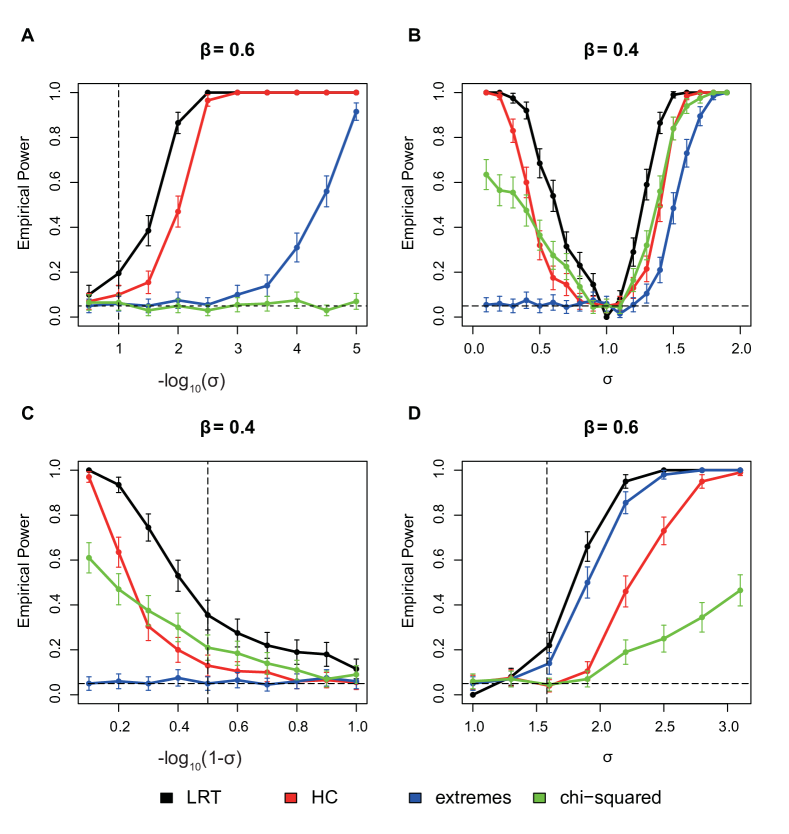
Figure 1: Empirical power comparison with 95% error bars. A. Sparse regime where $\beta=0.6$ and $\sigma\to 0$. B. Dense regime where $\beta=0.4$ and $\sigma$ fixed. Note that the LR test is here asymptotically powerful at any $\sigma\neq 1$. C. Dense regime where $\beta=0.4$ and $\sigma\to 1$. D. Sparse regime where $\beta=0.6$ and $\sigma>1$. Each time, the horizontal line marks the level (set at 0.05) and the vertical line marks the asymptotic detection boundary derived earlier in the paper.

References

• Anderson and Darling [1952] T. W. Anderson and D. A. Darling. Asymptotic theory of certain “goodness of fit” criteria based on stochastic processes. The Annals of Mathematical Statistics, 23(2):193–212, 1952.
• Cai and Wu [2014] T. T. Cai and Y. Wu. Optimal detection of sparse mixtures against a given null distribution. IEEE Transactions on Information Theory, 60(4):2217–2232, 2014.
• Cai et al. [2011] T. T. Cai, X. J. Jeng, and J. Jin. Optimal detection of heterogeneous and heteroscedastic mixtures. Journal of the Royal Statistical Society: Series B (Statistical Methodology), 73(5):629–662, 2011.
• Donoho and Jin [2004] D. Donoho and J. Jin. Higher criticism for detecting sparse heterogeneous mixtures. The Annals of Statistics, 32(3):962–994, 2004.
• Ingster [1997] Y. I. Ingster. Some problems of hypothesis testing leading to infinitely divisible distributions. Mathematical Methods of Statistics, 6(1):47–69, 1997.
• Jaeschke [1979] D. Jaeschke. The asymptotic distribution of the supremum of the standardized empirical distribution function on subintervals. The Annals of Statistics, 7(1):108–115, 1979.