Power Corrections for N-Jettiness Subtractions at ${\cal O}(\alpha_{s})\!\!$

Abstract

We continue the study of power corrections for $N$-jettiness subtractions by analytically computing the complete next-to-leading power corrections at ${\mathcal{O}}(\alpha_{s})$ for color-singlet production. This includes all nonlogarithmic terms and all partonic channels for Drell-Yan and gluon-fusion Higgs production. These terms are important to further improve the numerical performance of the subtractions, and to better understand the structure of power corrections beyond their leading logarithms, in particular their universality. We emphasize the importance of computing the power corrections differential in both the invariant mass, $Q$, and rapidity, $Y$, of the color-singlet system, which is necessary to account for the rapidity dependence in the subtractions. This also clarifies apparent disagreements in the literature. Performing a detailed numerical study, we find excellent agreement of our analytic results with a previous numerical extraction.

1 Introduction

The precision study of the Standard Model at the LHC, as well as increasingly sophisticated searches for physics beyond the Standard Model, require precision predictions for processes in a complicated hadron collider environment. When calculating higher-order QCD corrections, the presence of infrared divergences require techniques to isolate and cancel all divergences. Completely analytic calculations are only possible for some of the simplest cases, e.g. Anastasiou:2003ds ; Dulat:2017brz ; Mistlberger:2018etf , while for more complicated processes, in particular those involving jets in the final state, numerical techniques are typically required.

At next-to-leading order (NLO) the FKS Frixione:1995ms ; Frixione:1997np and CS Catani:1996jh ; Catani:1996vz ; Catani:2002hc subtraction schemes provide generic subtractions for arbitrary processes, and have been used to great success. At next-to-next-to-leading order (NNLO), due to the more complicated structure of infrared singularities, the development of general subtraction schemes has proven more difficult. While subtraction schemes have been demonstrated both for color-singlet production Catani:2007vq ; Caola:2017dug ; Herzog:2018ily ; Magnea:2018hab ; DelDuca:2016csb ; DelDuca:2016ily ; Kardos:2018kqd , as well as for several processes involving jets in the final state GehrmannDeRidder:2005cm ; Czakon:2010td ; Boughezal:2011jf ; Czakon:2014oma ; Boughezal:2015dva ; Boughezal:2015aha ; Gaunt:2015pea , significant work is still required before efficient NNLO subtractions can be achieved for arbitrary colored final states.

$N$-jettiness subtractions Boughezal:2015dva ; Gaunt:2015pea are based on the $N$-jettiness resolution variable $\mathcal{T}_{N}$ Stewart:2009yx ; Stewart:2010tn , and are applicable to generic $N$-jet final states. They have successfully been applied to NNLO calculations for a variety of color-singlet final states Campbell:2016jau ; Campbell:2016yrh ; Boughezal:2016wmq ; Campbell:2017aul ; Heinrich:2017bvg , as well as final states involving a single jet Boughezal:2015dva ; Boughezal:2015aha ; Boughezal:2015ded ; Boughezal:2016dtm ; Campbell:2017dqk ; Abelof:2016pby . They are also a key ingredient in one of the first methods for combining NNLO calculations with parton showers Alioli:2012fc ; Alioli:2015toa . The leading-power subtraction terms are given by an all-orders factorization formula derived in refs. Stewart:2009yx ; Stewart:2010tn using soft-collinear effective theory (SCET) Bauer:2000ew ; Bauer:2000yr ; Bauer:2001ct ; Bauer:2001yt ; Bauer:2002nz . Required ingredients are explicitly known to NNLO with up to a single jet in the final state Becher:2006qw ; Stewart:2010qs ; Becher:2010pd ; Berger:2010xi ; Jouttenus:2011wh ; Kelley:2011ng ; Monni:2011gb ; Hornig:2011iu ; Kang:2015moa ; Gaunt:2014xga ; Gaunt:2014cfa ; Boughezal:2015eha ; Li:2016tvb ; Boughezal:2017tdd ; Campbell:2017hsw .

An important feature of $N$-jettiness subtractions is that power corrections in the resolution variable can be calculated in an expansion about the soft and collinear limits, allowing the numerical performance of the subtractions to be systematically improved. Recently there has been significant interest in understanding subleading power corrections to collider cross sections Laenen:2008ux ; Laenen:2010uz ; Bonocore:2014wua ; Bonocore:2015esa ; Kolodrubetz:2016uim ; Bonocore:2016awd ; Moult:2016fqy ; Boughezal:2016zws ; Moult:2017jsg ; Moult:2017rpl ; Feige:2017zci ; DelDuca:2017twk ; Chang:2017atu ; Beneke:2017ztn ; Boughezal:2018mvf ; Bahjat-Abbas:2018hpv . Advances in the understanding of subleading power limits using SCET Moult:2017rpl ; Feige:2017zci have allowed the leading logarithmic (LL) next-to-leading power (NLP) corrections to be computed at NLO and NNLO Moult:2016fqy ; Moult:2017jsg , with independent calculations of the same terms done by a second group in refs. Boughezal:2016zws ; Boughezal:2018mvf . The leading logarithms have also been resummed to all orders for pure glue QCD for 2-jettiness in $H\to gg$ Moult:2018jjd .

The inclusion of the leading logarithms was found to improve the numerical accuracy, and thereby the computational efficiency, of $N$-jettiness subtractions for color-singlet production by up to an order of magnitude Moult:2016fqy ; Moult:2017jsg . The analytic calculation of the next-to-leading logarithmic (NLL) power corrections is important for several reasons. Theoretically, it greatly furthers our understanding of the power corrections, since the perturbative structure becomes significantly more nontrivial at NLL as compared to at LL. From a practical perspective, they provide further substantial improvements in the numerical performance of the subtractions. In particular, they make the subtractions much more robust in cases where there are accidental cancellations between different channels or where the NLL terms are numerically enhanced relative to the LL terms.

In this paper, we compute the full NLP corrections at ${\mathcal{O}}(\alpha_{s})$ for both Drell-Yan and gluon-fusion Higgs production in all partonic channels, including the nonlogarithmic terms (which are the NLL terms at ${\mathcal{O}}(\alpha_{s})$). One focus of this paper is to derive a master formula for the NLP corrections to $0$-jettiness at ${\mathcal{O}}(\alpha_{s})$ and to discuss in detail the subleading-power calculation, in particular the treatment of measurements at subleading power, which in our case are the invariant mass $Q$ and rapidity $Y$ of the color-singlet system. More generally, one can consider measuring any observable that does not vanish for the partonic process at lowest order in perturbation theory, which we refer to as Born measurements. Our analysis lays the ground for extending the calculation of the NLP corrections to higher powers, higher orders in $\alpha_{s}$, and to more complicated processes.

We also perform a detailed numerical study comparing our analytic results with the full nonsingular result extracted numerically from MCFM8 Campbell:1999ah ; Campbell:2010ff ; Campbell:2015qma ; Boughezal:2016wmq , which allows us both to verify our analytic calculation and to probe the typical size of the higher-power corrections in various different partonic channels. We find that the NLL power corrections can exhibit a much more pronounced $Y$ dependence from PDF effects than is the case at LL, which demonstrates the importance of calculating the power corrections fully differential in the Born phase space.

Our discussion of the Born measurements also allows us to clarify an apparent disagreement in the recent literature regarding the LL power corrections. As we discuss in more detail in sec. 6, since the calculations in refs. Boughezal:2016zws ; Boughezal:2018mvf are not differential in the color-singlet rapidity $Y$, their results can only be used fully integrated over $Y$. In contrast, the results computed here, which agree with those previously derived by a subset of the present authors in refs. Moult:2016fqy ; Moult:2017jsg , are differential in $Y$. When integrating over all $Y$, integration by parts is used to explicitly show that these LL results are equivalent to those of refs. Boughezal:2016zws ; Boughezal:2018mvf . In sec. 6 we also compare our new differential NLL results with the integrated results of ref. Boughezal:2018mvf .

The outline of this paper is as follows: In sec. 2, we briefly review $N$-jettiness subtractions for color-singlet production and define our notation. In sec. 3, we discuss in some detail the treatment of Born measurements at subleading power. In sec. 4, we derive a formula to NLP for the soft and collinear power corrections for $0$-jettiness. Although our primary focus is on NLO, the general strategy is valid to higher orders as well. In sec. 5, we use our master formula to derive explicit results for the NLP power corrections at NLO for both Drell-Yan and gluon-fusion Higgs production. In sec. 6, we provide a detailed comparison with the literature for those partonic channels where results are available. In sec. 7, we present a detailed numerical study, and compare our analytic results with a previous numerical extraction. We conclude in sec. 8.

2 N-Jettiness Subtractions, Definitions and Notation

In this section we briefly review $N$-jettiness subtractions Boughezal:2015dva ; Gaunt:2015pea in the context of color-singlet production, and discuss the structure of the power corrections to the subtraction scheme. This also allows us to define the notation that will be used in the rest of this paper. For a detailed discussion, we refer the reader to ref. Gaunt:2015pea .

To compute a cross section for color-singlet production $\sigma(X)$, where $X$ denotes some set of cuts on the Born phase space, we write the cross section as an integral over the differential cross section in the resolution variable $\mathcal{T}_{0}$

$$\sigma(X) =\sigma(X,\mathcal{T}_{\mathrm{cut}})+\int_{\mathcal{T}_{\mathrm{cut}}}\!\mathrm{d}\mathcal{T}_{0}\,\frac{\mathrm{d}\sigma(X)}{\mathrm{d}\mathcal{T}_{0}}\,,$$ (1)

where

$$\sigma(X,\mathcal{T}_{\mathrm{cut}}) \equiv\int^{\mathcal{T}_{\mathrm{cut}}}\!\mathrm{d}\mathcal{T}_{0}\,\frac{\mathrm{d}\sigma(X)}{\mathrm{d}\mathcal{T}_{0}}\,.$$ (2)

For a general measure, the 0-jettiness $\mathcal{T}_{0}$ can be defined as Stewart:2010pd ; Jouttenus:2011wh

$$\mathcal{T}_{0}=\sum_{i}\min\biggl{\{}\frac{2q_{a}\cdot k_{i}}{Q_{a}}\,,\frac{2q_{b}\cdot k_{i}}{Q_{b}}\biggr{\}}\,,$$ (3)

where the sum runs over all hadronic momenta $k_{i}$ in the final state. Here, $q_{a,b}$ are projected Born momenta (referred to as label momenta in SCET), which are given in terms of the total leptonic invariant mass $Q$ and rapidity $Y$ as

$$q_{a}^{\mu}=x_{a}E_{\mathrm{cm}}\frac{n^{\mu}}{2}=Qe^{Y}\frac{n^{\mu}}{2}\,,\qquad q_{b}^{\mu}=x_{b}E_{\mathrm{cm}}\frac{\bar{n}^{\mu}}{2}=Qe^{-Y}\frac{\bar{n}^{\mu}}{2}\,,$$ (4)

where

$$n^{\mu}=(1,0,0,1)\,,\quad\bar{n}^{\mu}=(1,0,0,-1)$$ (5)

are lightlike vectors along the beam directions. The choice in eq. (4) corresponds to parameterizing the Born phase space in terms of $Q$ and $Y$, and this choice already enters in the leading-power factorization theorem, where the beam functions are evaluated at $x_{a,b}=Qe^{\pm Y}$.

The $Q_{a,b}$ measures in eq. (3) determine the different definitions of 0-jettiness. Two different definitions, originally introduced in refs. Stewart:2009yx ; Berger:2010xi as beam thrust, are the leptonic and hadronic definitions given by

leptonic: $$Q_{a} =Q_{b}=Q\,,\qquad \mathcal{T}_{0}^{\mathrm{lep}} =\sum_{i}\min\biggl{\{}\frac{x_{a}E_{\mathrm{cm}}}{Q}n\cdot k_{i}\,,\,\frac{x_{b}E_{\mathrm{cm}}}{Q}\bar{n}\cdot k_{i}\biggr{\}}$$

$$=\sum_{i}\min\biggl{\{}e^{Y}n\cdot k_{i}\,,\,e^{-Y}\bar{n}\cdot k_{i}\biggr{\}}$$

hadronic: $$Q_{a,b} =x_{a,b}E_{\mathrm{cm}}\,, \mathcal{T}_{0}^{\mathrm{cm}} =\sum_{i}\min\Bigl{\{}n\cdot k_{i}\,,\,\bar{n}\cdot k_{i}\Bigr{\}}\,.$$ (6)

It has been shown Moult:2016fqy that the power corrections for the hadronic definition are poorly behaved, and grow exponentially with rapidity, while the $e^{\pm Y}$ factor in the measure for the leptonic definition exactly avoids this effect.

For later convenience, we write the dimensionful and dimensionless $0$-jettiness resolution variables in terms of a $Y$-dependent parameter $\rho(Y)$ as

$$\mathcal{T}_{0}^{x} =\sum_{i}\min\Bigl{\{}\rho_{x}\,k_{i}^{+},\rho_{x}^{-1}\,k_{i}^{-}\Bigr{\}}\,,\qquad\tau^{x}\equiv\frac{\mathcal{T}_{0}^{x}}{Q}\,,$$ (7)

with

leptonic: $$\rho_{\mathrm{lep}}=e^{Y}\,,\qquad\tau^{\mathrm{lep}}=\frac{\mathcal{T}_{0}^{\mathrm{lep}}}{Q}\,,$$

hadronic: $$\rho_{\mathrm{cm}}=1\,,\qquad\tau^{\mathrm{cm}}=\frac{\mathcal{T}_{0}^{\mathrm{cm}}}{Q}\,.$$ (8)

In the following, we will mostly drop the subscript $0$ on $\mathcal{T}_{0}$, since there should be no cause for confusion that our results are for 0-jettiness. For generic results that apply to both the leptonic and hadronic definitions we also drop the superscript and simply use $\mathcal{T}$ and $\tau$, keeping a generic parameter $\rho$ when necessary.

To implement the $N$-jettiness subtractions, we now add and subtract a subtraction term to the cross section (suppressing the dependence on the Born measurements $X$ for simplicity)

$$\sigma =\sigma^{\mathrm{sub}}(\mathcal{T}_{{\mathrm{cut}}})+\int_{\mathcal{T}_{\mathrm{cut}}}\!\mathrm{d}\mathcal{T}_{0}\,\frac{\mathrm{d}\sigma}{\mathrm{d}\mathcal{T}_{0}}+\bigl{[}\sigma(\mathcal{T}_{\mathrm{cut}})-\sigma^{\mathrm{sub}}(\mathcal{T}_{\mathrm{cut}})\bigr{]}$$

$$\equiv\sigma^{\mathrm{sub}}(\mathcal{T}_{\mathrm{cut}})+\int_{\mathcal{T}_{\mathrm{cut}}}\!\mathrm{d}\mathcal{T}_{0}\,\frac{\mathrm{d}\sigma}{\mathrm{d}\mathcal{T}_{0}}+\Delta\sigma(\mathcal{T}_{\mathrm{cut}})\,.$$ (9)

Since $\mathcal{T}_{0}$ is a zero jet resolution variable, for $\tau=\mathcal{T}_{0}/Q\to 0$ we can expand the differential cross section $\mathrm{d}\sigma/\mathrm{d}\tau$ and its cumulative $\sigma(\tau_{\mathrm{cut}})$ about the soft and collinear limits from $\tau\to 0$ and $\tau_{\mathrm{cut}}\to 0$ as

$$\frac{\mathrm{d}\sigma}{\mathrm{d}\tau} =\frac{\mathrm{d}\sigma^{(0)}}{\mathrm{d}\tau}+\frac{\mathrm{d}\sigma^{(2)}}{\mathrm{d}\tau}+\frac{\mathrm{d}\sigma^{(4)}}{\mathrm{d}\tau}+\dotsb\,,$$ (10)

$$\sigma(\tau_{\mathrm{cut}}) =\sigma^{(0)}(\tau_{\mathrm{cut}})+\sigma^{(2)}(\tau_{\mathrm{cut}})+\sigma^{(4)}(\tau_{\mathrm{cut}})+\dotsb\,.$$

Here $\mathrm{d}\sigma^{(0)}/\mathrm{d}\tau$ and $\sigma^{(0)}(\tau_{\mathrm{cut}})$ contain all leading-power terms,

$$\frac{\mathrm{d}\sigma^{(0)}}{\mathrm{d}\tau}\sim\delta(\tau)+\biggl{[}\frac{\ln^{j}\tau}{\tau}\biggr{]}_{+}\,,\qquad\sigma^{(0)}(\tau_{\mathrm{cut}})\sim\ln^{j}\tau_{\mathrm{cut}}\,.$$ (11)

These terms must be included in the subtraction term to obtain a finite result, namely

$$\sigma^{\mathrm{sub}}(\mathcal{T}_{\mathrm{cut}})=\sigma^{(0)}(\tau_{\mathrm{cut}}=\mathcal{T}_{\mathrm{cut}}/Q)\,[1+\mathcal{O}(\tau_{\mathrm{cut}})]\,.$$ (12)

The further terms in the series expansion in eq. (10) are suppressed by powers of $\tau$

$$\tau\frac{\mathrm{d}\sigma^{(2k)}}{\mathrm{d}\tau} \sim\mathcal{O}(\tau^{k}\ln^{j}\tau)\,,\qquad\sigma^{(2k)}(\tau_{\mathrm{cut}})\sim\mathcal{O}(\tau_{\mathrm{cut}}^{k}\ln^{j}\tau_{\mathrm{cut}})\,.$$ (13)

While these terms with $k\geq 1$ do not need to be included in the subtraction term, the size of the neglected term, $\Delta\sigma(\tau_{\mathrm{cut}})$ is determined by the leading-power corrections that are left out of $\sigma^{\rm sub}$. Therefore, including additional power corrections in $\sigma^{\rm sub}$ can significantly improve the performance of the subtraction. Indeed, general scaling arguments imply that up to an order of magnitude in performance can be gained for each subleading power logarithm that is included in the subtractions Gaunt:2015pea . For the leading logarithms, this was explicitly confirmed for most partonic channels in the numerical studies in refs. Moult:2016fqy ; Moult:2017jsg . Here, we extend the calculation to the NLL terms at ${\mathcal{O}}(\alpha_{s})$, which yields the nonlogarithmic terms, hence giving the complete NLP result. The remaining NLO power corrections then scale at worst as $\alpha_{s}\tau_{{\mathrm{cut}}}^{2}\log\tau_{{\mathrm{cut}}}$, and will be very small, as we will see in our numerical studies.

3 Born Measurements at Subleading Power

We begin by discussing in some detail the treatment of the Born measurements, $Q^{2}$ and $Y$, which plays an important role at subleading powers. We will use the soft and collinear expansions from SCET, which provide a convenient language when discussing the power expansion of QCD amplitudes at fixed order. We will not need to employ any of the field theory technology from SCET for our analysis here.

3.1 General Setup and Notation

Consider the production of a color-singlet final state $L$ of fixed invariant mass $Q$ and rapidity $Y$, together with an arbitrary measurement $\mathcal{T}$ that only acts on hadronic radiation and gives $\mathcal{T}=0$ at Born level. Since the observable $\mathcal{T}$ resolves soft and collinear emissions it will induce large logarithms $\ln(\mathcal{T}/Q)$. Our goal is to expand the cross section in $\mathcal{T}$ (or $\tau=\mathcal{T}/Q$) in order to systematically understand its logarithmic structure.

Consider proton-proton scattering with the underlying partonic process

$$a(p_{a})+b(p_{b})\to L(p_{1},\cdots)+X(k_{1},\cdots)\,,$$ (14)

where $L$ is the leptonic (color-singlet) final state and $X$ denotes additional QCD radiation. Its cross section reads

$$\frac{\mathrm{d}\sigma}{\mathrm{d}Q^{2}\mathrm{d}Y\mathrm{d}\mathcal{T}} =\int_{0}^{1}\!\!\mathrm{d}\zeta_{a}\mathrm{d}\zeta_{b}\,\frac{f_{a}(\zeta_{a})\,f_{b}(\zeta_{b})}{2\zeta_{a}\zeta_{b}E_{\mathrm{cm}}^{2}}\int\!\biggl{(}\prod_{i}\frac{\mathrm{d}^{d}k_{i}}{(2\pi)^{d}}(2\pi)\delta_{+}(k_{i}^{2})\biggr{)}\int\!\!\frac{\mathrm{d}^{d}q}{(2\pi)^{d}}\,|{\mathcal{M}}(p_{a},p_{b};\{k_{i}\},q)|^{2}$$

$$\quad\times(2\pi)^{d}\delta^{(d)}(p_{a}+p_{b}-k-q)\,\delta(Q^{2}-q^{2})\,\delta\biggl{(}Y-\frac{1}{2}\ln\frac{q^{-}}{q^{+}}\biggr{)}\,\delta\bigl{[}\mathcal{T}-\hat{\mathcal{T}}(\{k_{i}\})\bigr{]}\,.$$ (15)

Here, the incoming momenta are given by

$$p_{a}^{\mu}=\zeta_{a}E_{\mathrm{cm}}\frac{n^{\mu}}{2}\,,\qquad p_{b}^{\mu}=\zeta_{b}E_{\mathrm{cm}}\frac{\bar{n}^{\mu}}{2}\,,$$ (16)

$k=\sum_{i}k_{i}$ is the total outgoing hadronic momentum, and $q$ is the total leptonic momentum. Since our measurements are not sensitive to the details of the leptonic final state, we have absorbed the leptonic phase space integral into the matrix element,

$$|{\mathcal{M}}(p_{a},p_{b};\{k_{i}\},q)|^{2} =\int\mathrm{d}\Phi_{L}(q)\,|{\mathcal{M}}(p_{a},p_{b};\{k_{i}\},\{p_{j}\})|^{2}\,,$$

$$\mathrm{d}\Phi_{L}(q) =\prod_{j}\frac{\mathrm{d}^{d}p_{j}}{(2\pi)^{d}}(2\pi)\delta_{+}(p_{j}^{2}-m_{j}^{2})\,(2\pi)^{d}\delta^{(d)}\Bigl{(}q-\sum_{j}p_{j}\Bigr{)}\,.$$ (17)

The matrix element ${\mathcal{M}}$ contains the renormalization scale $\mu^{2\epsilon}$, which as always is associated with the renormalized coupling $\alpha_{s}(\mu)$, and may also contain virtual corrections. For now the measurement function $\hat{\mathcal{T}}(\{k_{i}\})$ is kept arbitrary.

We can now solve the $Q^{2}$ and $Y$ measurements to fix the incoming momenta as

$$\zeta_{a}(k) =\frac{1}{E_{\mathrm{cm}}}\biggl{(}k^{-}+e^{+Y}\sqrt{Q^{2}+k_{T}^{2}}\biggr{)}\,,$$

$$\zeta_{b}(k) =\frac{1}{E_{\mathrm{cm}}}\biggl{(}k^{+}+e^{-Y}\sqrt{Q^{2}+k_{T}^{2}}\biggr{)}\,.$$ (18)

Taking the Jacobian factors from solving the $\delta$ functions into account, eq. (3.1) becomes

$$\frac{\mathrm{d}\sigma}{\mathrm{d}Q^{2}\mathrm{d}Y\mathrm{d}\mathcal{T}} =\int\!\biggl{(}\prod_{i}\frac{\mathrm{d}^{d}k_{i}}{(2\pi)^{d}}(2\pi)\delta_{+}(k_{i}^{2})\biggr{)}\frac{f_{a}(\zeta_{a})\,f_{b}(\zeta_{b})}{2\zeta_{a}\zeta_{b}E_{\mathrm{cm}}^{4}}A(Q,Y;\{k_{i}\})\delta\bigl{[}\mathcal{T}-\hat{\mathcal{T}}(\{k_{i}\})\bigr{]}\,,$$ (19)

where we defined

$$A(Q,Y;\{k_{i}\})\equiv|{\mathcal{M}}(p_{a},p_{b},\{k_{i}\},q=p_{a}+p_{b}-k)|^{2}$$ (20)

to stress that the squared matrix element only depends on the Born measurements $Q$ and $Y$, which fix the incoming momenta through eqs. (16) and (3.1), and the emission momenta $k_{i}$. Note that we have left implicit in our notation in eq. (19) the dependence of $\zeta_{a,b}$ on $k$ through eq. (3.1). They are restricted to $\zeta_{a,b}\in[0,1]$, which is implicit in the support of the proton PDFs.

3.2 Power Expansion in Soft and Collinear Limits

Instead of solving the $\mathcal{T}$ measurement function to express (some of the) $k_{i}$ in terms of $\mathcal{T}$, we find that a convenient strategy to organize the expansion in $\mathcal{T}$ is to multipole expand the final state momenta. At this stage we need only assume that $\mathcal{T}$ is a $\text{SCET}_{\text{I}}$ observable, which is true for many definitions of $N$-jettiness. For such observables, it is known from $\text{SCET}_{\text{I}}$ that we can organize the cross section in terms of a power counting parameter $\lambda\sim\sqrt{\tau}$. All momenta $k_{i}$ can then be categorized as either collinear or soft modes (since we work in $\text{SCET}_{\text{I}}$ these are often called ultrasoft, although we will not make this distinction), whose momenta scale as

$$n{-}\text{collinear}:\quad k_{n}\sim Q\,(\lambda^{2},1,\lambda)\,,$$ (21)

$$\bar{n}{-}\text{collinear}:\quad k_{\bar{n}}\sim Q\,(1,\lambda^{2},\lambda)\,,$$

$$\text{soft}:\hskip 51.21504ptk_{s}\sim Q\,(\lambda^{2},\lambda^{2},\lambda^{2})\,,$$

where we decomposed each momentum into lightcone coordinates

$$k^{\mu}=k^{-}\frac{n^{\mu}}{2}+k^{+}\frac{\bar{n}^{\mu}}{2}+k_{\perp}^{\mu}\equiv(k^{+},k^{-},k_{\perp})\,.$$ (22)

Here $n$ and $\bar{n}$ are lightlike vectors satisfying $n\cdot\bar{n}=2$. The components of the momenta that scale like $\lambda^{2}$ are referred to as residual momenta. The soft momenta are homogeneous, and have purely residual scaling. Overlap between the soft and collinear modes occurring in integrals over final state momenta is removed by the zero-bin subtraction procedure Manohar:2006nz .

The benefit of this decomposition is that it allows one to expand eq. (19) in $\lambda$, agnostic of the actual measurement $\mathcal{T}$. The LP result is then simply obtained by expanding the cross section through $\lambda^{0}$, the NLP result by expanding through $\lambda^{2}$, etc. Note that when performing this expansion, all other factors, such as $Q,E_{\rm cm}\sim\lambda^{0}$.

While the expansion of the matrix element is of course process dependent, we can give general expressions for the incoming momentum fractions eq. (3.1), independent of the process and observable $\mathcal{T}$. If $k$ is a soft momentum, then the expansion required at NLP is given by

$$\zeta_{a}(k) =x_{a}\biggl{(}1+\frac{k^{-}e^{-Y}}{Q}\biggr{)}+{\mathcal{O}}(\lambda^{4})\,,$$

$$\zeta_{b}(k) =x_{b}\biggl{(}1+\frac{k^{+}e^{+Y}}{Q}\biggr{)}+{\mathcal{O}}(\lambda^{4})\,,$$ (23)

where we factored out the Born momentum fractions

$$x_{a}=\frac{Qe^{+Y}}{E_{\mathrm{cm}}}\,,\qquad x_{b}=\frac{Qe^{-Y}}{E_{\mathrm{cm}}}\,.$$ (24)

In the $n$-collinear limit, we obtain

$$\zeta_{a}(k) =x_{a}\biggl{[}\biggl{(}1+\frac{k^{-}e^{-Y}}{Q}\biggr{)}+\frac{k_{T}^{2}}{2Q^{2}}\biggr{]}+{\mathcal{O}}(\lambda^{4})\,,$$

$$\zeta_{b}(k) =x_{b}\biggl{[}1+\biggl{(}\frac{k^{+}e^{+Y}}{Q}+\frac{k_{T}^{2}}{2Q^{2}}\biggr{)}\biggr{]}+{\mathcal{O}}(\lambda^{4})\,.$$ (25)

For clarity, we have grouped terms of the same power counting in round brackets. Similarly, one can obtain the $\bar{n}$-collinear limit, or any combination as might appear when combining multiple emissions.

4 Master Formula for Power Corrections to Next-to-Leading Power

In this section we derive a master formula for the NLP corrections. This formula applies to any $\text{SCET}_{\text{I}}$ observable in color-singlet production. In sec. 5, we will apply it to derive explicit results for Drell-Yan and gluon-fusion Higgs production.

4.1 General Setup for Color-Singlet $\text{SCET}_{\text{I}}$ Observables

For reference, we start with the LO cross section for the production of a color-singlet final state $L$ of invariant mass $Q^{2}$ and rapidity $Y$, together with an (up to now arbitrary) measurement $\mathcal{T}$ acting only on hadronic radiation,

$$\frac{\mathrm{d}\sigma^{\mathrm{LO}}}{\mathrm{d}Q^{2}\mathrm{d}Y\mathrm{d}\mathcal{T}} =\frac{f_{a}(x_{a})\,f_{b}(x_{b})}{2x_{a}x_{b}E_{\mathrm{cm}}^{4}}A^{\mathrm{LO}}(Q,Y)\,\delta(\mathcal{T})\,,$$ (26)

where $x_{a,b}=\frac{Q}{E_{\mathrm{cm}}}e^{\pm Y}$ and $A^{\mathrm{LO}}$ is the squared matrix element in the Born kinematics, see eq. (20). For future reference, we also define the LO partonic cross section, $\hat{\sigma}^{\rm LO}(Q,Y)$, by

$$\frac{\mathrm{d}\sigma^{\mathrm{LO}}}{\mathrm{d}Q^{2}\mathrm{d}Y\mathrm{d}\mathcal{T}} =\hat{\sigma}^{\mathrm{LO}}(Q,Y)\,f_{a}(x_{a})\,f_{b}(x_{b})\,\delta(\mathcal{T})\,,\qquad\hat{\sigma}^{\mathrm{LO}}(Q,Y)=\frac{A^{\mathrm{LO}}(Q,Y)}{2x_{a}x_{b}E_{\mathrm{cm}}^{4}}\,.$$ (27)

Next, consider an additional real emission to the Born process. Eq. (19) yields

$$\frac{\mathrm{d}\sigma}{\mathrm{d}Q^{2}\mathrm{d}Y\mathrm{d}\mathcal{T}} =\int\!\frac{\mathrm{d}^{d}k}{(2\pi)^{d}}\,(2\pi)\delta_{+}(k^{2})\,\frac{f_{a}(\zeta_{a})\,f_{b}(\zeta_{b})}{2\zeta_{a}\zeta_{b}E_{\mathrm{cm}}^{4}}\,A(Q,Y;\{k\})\,\delta\bigl{[}\mathcal{T}-\hat{\mathcal{T}}(\{k\})\bigr{]}\,,$$ (28)

where we remind the reader that the incoming momenta $p_{a,b}$ are given by eq. (3.1),

$$p_{a}^{\mu} =\zeta_{a}(k)E_{\mathrm{cm}}\frac{n^{\mu}}{2}=\biggl{(}k^{-}+e^{+Y}\sqrt{Q^{2}+k_{T}^{2}}\biggr{)}\frac{n^{\mu}}{2}\,,$$

$$p_{b}^{\mu} =\zeta_{b}(k)E_{\mathrm{cm}}\frac{\bar{n}^{\mu}}{2}=\biggl{(}k^{+}+e^{-Y}\sqrt{Q^{2}+k_{T}^{2}}\biggr{)}\frac{\bar{n}^{\mu}}{2}\,.$$ (29)

From these solutions, we see the interesting feature that at subleading power, regardless of the type of final-state emission, the momenta entering both PDFs are modified.

Since we do not measure the azimuthal angle of $k$, it can be integrated over,

$$\int\!\frac{\mathrm{d}^{d}k}{(2\pi)^{d}}\,(2\pi)\delta_{+}(k^{2})=\frac{\Omega_{2-2\epsilon}}{4(2\pi)^{d-1}}\int_{0}^{\infty}\frac{\mathrm{d}k^{+}\mathrm{d}k^{-}}{(k^{+}k^{-})^{\epsilon}}=\frac{(4\pi)^{-2+\epsilon}}{\Gamma(1-\epsilon)}\int_{0}^{\infty}\frac{\mathrm{d}k^{+}\mathrm{d}k^{-}}{(k^{+}k^{-})^{\epsilon}}\,.$$ (30)

Eq. (28) simplifies to

$$\frac{\mathrm{d}\sigma}{\mathrm{d}Q^{2}\mathrm{d}Y\mathrm{d}\mathcal{T}} =\int_{0}^{\infty}\frac{\mathrm{d}k^{+}\mathrm{d}k^{-}}{(k^{+}k^{-})^{\epsilon}}\frac{f_{a}(\zeta_{a})\,f_{b}(\zeta_{b})}{(4\pi)^{2}2\zeta_{a}\zeta_{b}E_{\mathrm{cm}}^{4}}\,\frac{(4\pi)^{\epsilon}}{\Gamma(1-\epsilon)}\,A(Q,Y;\{k\})\,\delta\bigl{[}\mathcal{T}-\hat{\mathcal{T}}(\{k\})\bigr{]}\,.$$ (31)

So far, this expression is still exact. In the next step, we wish to expand the NLO cross section in $\lambda\sim\mathcal{T}/Q$. When $\mathcal{T}$ is a $\text{SCET}_{\text{I}}$ observable, we can use the EFT knowledge from $\text{SCET}_{\text{I}}$ to expand the momentum $k$ in both collinear and soft limits, as discussed in sec. 3.

At NLP, we need to expand eq. (31) consistently through ${\mathcal{O}}(\lambda^{2})$. The ${\mathcal{O}}(\lambda^{2})$ power corrections arise from the following sources:

• The incoming momenta $\zeta_{a,b}$: While collinear and soft limits yield quite different power expansions, both give a well-defined expansion in $\lambda$. We thus simply define the expansion

  $$\zeta_{a,b}=x_{a,b}\biggl{[}\frac{1}{z_{a,b}}+\Delta_{a,b}^{(2)}+{\mathcal{O}}(\lambda^{4})\biggr{]}\,,$$ (32)

  where $z_{a,b}\sim\lambda^{0}$ and $\Delta_{a,b}^{(2)}\sim\lambda^{2}$. We have pulled out the Born momentum fractions $x_{a,b}$ and written $1/z_{a,b}$ as a fraction for later convenience. Explicit expressions can be obtained from eqs. (3.2) and (3.2), and will be given below.

• PDFs: Since the momenta $\zeta_{a,b}$ enter the PDFs, these also have to be power expanded,

  $$f_{a,b}(\zeta_{a,b}) =f_{a,b}\biggl{(}\frac{x_{a,b}}{z_{a,b}}\biggr{)}+x_{a,b}\Delta_{a,b}^{(2)}\,f^{\prime}_{a,b}\biggl{(}\frac{x_{a,b}}{z_{a,b}}\biggr{)}+{\mathcal{O}}(\lambda^{4})$$

  $$\equiv f_{a,b}+x_{a,b}\Delta_{a,b}^{(2)}\,f^{\prime}_{a,b}+{\mathcal{O}}(\lambda^{4})\,.$$ (33)

• Flux factor: Similar to the PDFs, we have to expand the flux factor

  $$\frac{1}{\zeta_{a}\zeta_{b}}=\frac{z_{a}z_{b}}{x_{a}x_{b}}\biggl{[}1-z_{a}\Delta^{(2)}-z_{b}\Delta^{(2)}_{b}\biggr{]}\,.$$ (34)

• Matrix element: The expansion of the matrix element depends both on the process and the considered limit. Here, we define the LP and NLP expansions by

  $$A(Q,Y;\{k\})=A^{(0)}(Q,Y;\{k\}))+A^{(2)}(Q,Y;\{k\})+\cdots\,.$$ (35)

  In the soft limit $A^{(0)}\sim\lambda^{-4}$ and $A^{(2)}\sim\lambda^{-2}$, while in the collinear limit $A^{(0)}\sim\lambda^{-2}$ and $A^{(2)}\sim\lambda^{0}$. In both cases we have the scaling $\int\mathrm{d}k^{+}\mathrm{d}k^{-}A^{(2j)}\sim\lambda^{2j}$, which is why the soft and collinear corrections enter at the same order.

  For example, for a $2\to 2$ process, the matrix element can be written in terms of the Mandelstam variables

  $$s_{ab} =2p_{a}\cdot p_{b}=\frac{Q^{2}}{z_{a}z_{b}}\left[1+z_{a}\Delta^{(2)}_{a}+z_{b}\Delta^{(2)}_{b}+{\mathcal{O}}(\lambda^{4})\right]\,,$$

  $$s_{ak} =-2p_{a}\cdot k=-k^{+}Qe^{+Y}\left(\frac{1}{z_{a}}+\Delta^{(2)}_{a}+{\mathcal{O}}(\lambda^{4})\right)\,,$$

  $$s_{bk} =-2p_{b}\cdot k=-k^{-}Qe^{-Y}\left(\frac{1}{z_{b}}+\Delta^{(2)}_{b}+{\mathcal{O}}(\lambda^{4})\right)\,.$$ (36)

  Since these terms now have a definite power counting, one can simply insert eq. (• ‣ 4.1) into $A(Q,Y;\{k\})$ and expand to the required order in $\lambda$.

• Measurement: Depending on the observable, the measurement function $\hat{\mathcal{T}}$ may also receive power corrections. Since $0$-jettiness is defined in terms of $n$, $\bar{n}$, $Q$ and $Y$, none of which receive power corrections in our approach, we do not have such corrections, and will therefore not write them explicitly in the following formulae. More generally, these could be obtained from expanding $\delta\bigl{[}\mathcal{T}-\hat{\mathcal{T}}(\{k\})\bigr{]}$.

Inserting all these expansions into eq. (31) and expanding consistently to ${\mathcal{O}}(\lambda^{2})$, we obtain the LP result

$$\frac{\mathrm{d}\sigma^{(0)}}{\mathrm{d}Q^{2}\mathrm{d}Y\mathrm{d}\mathcal{T}} =\int_{0}^{\infty}\frac{\mathrm{d}k^{+}\mathrm{d}k^{-}}{(k^{+}k^{-})^{\epsilon}}\frac{z_{a}z_{b}\,f_{a}f_{b}}{(4\pi)^{2}2x_{a}x_{b}E_{\mathrm{cm}}^{4}}\frac{(4\pi)^{\epsilon}}{\Gamma(1-\epsilon)}A^{(0)}(Q,Y;\{k\})\,\delta\bigl{[}\mathcal{T}-\hat{\mathcal{T}}(\{k\})\bigr{]}$$ (37)

and the NLP master formula

$$\frac{\mathrm{d}\sigma^{(2)}}{\mathrm{d}Q^{2}\mathrm{d}Y\mathrm{d}\mathcal{T}} =\int_{0}^{\infty}\frac{\mathrm{d}k^{+}\mathrm{d}k^{-}}{(k^{+}k^{-})^{\epsilon}}\frac{z_{a}z_{b}}{(4\pi)^{2}2x_{a}x_{b}E_{\mathrm{cm}}^{4}}\frac{(4\pi)^{\epsilon}}{\Gamma(1-\epsilon)}\delta\bigl{[}\mathcal{T}-\hat{\mathcal{T}}(\{k\})\bigr{]}$$

$$\quad\times\Bigl{\{}A^{(0)}(Q,Y;\{k\})\Bigl{[}f_{a}f_{b}\Bigl{(}-z_{a}\Delta_{a}^{(2)}-z_{b}\Delta_{b}^{(2)}\Bigr{)}+x_{a}\Delta_{a}^{(2)}f^{\prime}_{a}f_{b}+x_{b}\Delta_{b}^{(2)}f_{a}f^{\prime}_{b}\Bigr{]}$$

$$\qquad+f_{a}f_{b}\,A^{(2)}(Q,Y;\{k\})\Bigr{\}}\,,$$ (38)

where $z_{a,b}\equiv z_{a,b}(k)$ and $\Delta_{a,b}^{(2)}\equiv\Delta_{a,b}^{(2)}(k)$ are defined by eq. (32). Note that the LP limits of the matrix elements are universal, and hence eq. (37) holds independently of the process, i.e. it only depends on the observable $\mathcal{T}$. Although the focus of this paper is on the power corrections, in appendix A we provide a brief derivation of the leading-power terms. Likewise, the $A^{(0)}$ term together with the square bracketed factor on the second line of eq. (4.1) is universal, such that all the process dependence arises from the last $A^{(2)}$ term. We will discuss this in more detail in sec. 4.4.

In the following, we will evaluate eq. (4.1) in both the soft and collinear limit for $0$-jettiness, eq. (7), whose measurement function for one emission is given by

$$\delta\bigl{[}\mathcal{T}-\hat{\mathcal{T}}(k)\bigr{]}=\Theta(\rho k^{+}-\rho^{-1}k^{-})\delta(\mathcal{T}-\rho^{-1}k^{-})+\Theta(\rho^{-1}k^{-}-\rho k^{+})\delta(\mathcal{T}-\rho k^{+})\,.$$ (39)

The value of $\rho$ depends on the specific definition of $\mathcal{T}$, as given in eq. (2).

4.2 Collinear Master Formula for 0-Jettiness

The expansion of the incoming momenta $\zeta_{a,b}$ for an $n$-collinear emission $k\sim(\lambda^{2},1,\lambda)$ has been given in eq. (3.2),

$$\zeta_{a}(k) =x_{a}\biggl{[}\biggl{(}1+\frac{k^{-}e^{-Y}}{Q}\biggr{)}+\frac{k_{T}^{2}}{2Q^{2}}\biggr{]}+{\mathcal{O}}(\lambda^{4})\,,$$

$$\zeta_{b}(k) =x_{b}\biggl{[}1+\biggl{(}\frac{k^{+}e^{+Y}}{Q}+\frac{k_{T}^{2}}{2Q^{2}}\biggr{)}\biggr{]}+{\mathcal{O}}(\lambda^{4})\,,$$ (40)

so the explicit expressions for the expansion eq. (32) are

$$z_{a} =\biggl{(}1+\frac{k^{-}e^{-Y}}{Q}\biggr{)}^{-1}\,,\quad \Delta^{(2)}_{a}=\frac{k_{T}^{2}}{2Q^{2}}\,,$$

$$z_{b} =1\,,\quad \Delta^{(2)}_{b}=\biggl{(}\frac{k^{+}e^{+Y}}{Q}+\frac{k_{T}^{2}}{2Q^{2}}\biggr{)}\,.$$ (41)

Since an $n$-collinear emission satisfies $k^{-}\gg k^{+}$, the 0-jettiness measurement eq. (39) simplifies to

$$\delta\bigl{[}\mathcal{T}-\hat{\mathcal{T}}(k)\bigr{]}=\delta(\mathcal{T}-\rho k^{+})\,.$$ (42)

Note that the integration in eq. (4.1) also includes the region $k^{-}\to 0$, where the assumption $k^{-}\gg k^{+}$ is invalid. Indeed, this region corresponds to the soft expansion. It is guaranteed by the zero-bin subtraction procedure that this overlap regime between the soft and collinear limits is not double counted Manohar:2006nz . An important benefit of $0$-jettiness and our setup here is that the zero-bin contribution that removes the overlap is scaleless and vanishes in pure dimensional regularization, such that we do not need to consider it further.

Eq. 42 fixes the $k^{+}$ integral in eq. (4.1). It is also useful to write the remaining $k^{-}$ integration in terms of $z_{a}$ using eq. (4.2), giving

$$k^{-}=Qe^{Y}\frac{1-z_{a}}{z_{a}}\,,\qquad\int_{0}^{\infty}\mathrm{d}k^{-}=\int_{x_{a}}^{1}\frac{\mathrm{d}z_{a}}{z_{a}^{2}}\,Qe^{Y}\,.$$ (43)

Here the lower bound on the integration follows from the physical support of the PDF $f_{a}(x_{a}/z_{a})$. Plugging back into eq. (4.1), we obtain the $n$-collinear master formula

$$\frac{\mathrm{d}\sigma_{n}^{(2)}}{\mathrm{d}Q^{2}\mathrm{d}Y\mathrm{d}\mathcal{T}} =\int_{x_{a}}^{1}\frac{\mathrm{d}z_{a}}{z_{a}}\,\frac{1}{2x_{a}x_{b}E_{\mathrm{cm}}^{4}}\frac{Qe^{Y}}{\rho}\biggl{(}\frac{Q\mathcal{T}e^{Y}}{\rho}\biggr{)}^{-\epsilon}\frac{z_{a}^{\epsilon}}{(1-z_{a})^{\epsilon}}\frac{(4\pi)^{\epsilon}}{(4\pi)^{2}\Gamma(1-\epsilon)}$$

$$\quad\times\biggl{\{}\frac{\mathcal{T}e^{Y}}{Q\rho}A^{(0)}(Q,Y,\{k\})\biggl{[}f_{a}\,f_{b}\,\frac{(1-z_{a})^{2}-2}{2z_{a}}+\frac{1-z_{a}}{2z_{a}}\,x_{a}f^{\prime}_{a}\,f_{b}+\frac{1+z_{a}}{2z_{a}}\,f_{a}\,x_{b}f^{\prime}_{b}\biggr{]}$$

$$\qquad+f_{a}\,f_{b}\,A^{(2)}(Q,Y,\{k\})\biggr{\}}\,,$$ (44)

where $k$ is given by

$$k^{\mu}=Qe^{Y}\frac{1-z_{a}}{z_{a}}\frac{n^{\mu}}{2}+\frac{\mathcal{T}}{\rho}\frac{\bar{n}^{\mu}}{2}+\sqrt{Q\mathcal{T}\frac{e^{Y}}{\rho}\frac{1-z_{a}}{z_{a}}}n_{\perp}^{\mu}\,.$$ (45)

It only remains to plug in the expansions of the matrix element $A^{(0)}$ and $A^{(2)}$ and to expand in $\epsilon$. Note that even in the $n$-collinear case considered here, both the $n$ and $\bar{n}$-collinear incoming momenta receive power corrections, see eq. (4.1), leading to derivatives of both PDFs in eq. (4.2).

The analogous results for the $\bar{n}$-collinear limit are obtained in the same manner, giving

$$\frac{\mathrm{d}\sigma_{\bar{n}}^{(2)}}{\mathrm{d}Q^{2}\mathrm{d}Y\mathrm{d}\mathcal{T}} =\int_{x_{b}}^{1}\frac{\mathrm{d}z_{b}}{z_{b}}\,\frac{1}{2x_{a}x_{b}E_{\mathrm{cm}}^{4}}\frac{Q\rho}{e^{Y}}\biggl{(}\frac{Q\mathcal{T}\rho}{e^{Y}}\biggr{)}^{-\epsilon}\frac{z_{b}^{\epsilon}}{(1-z_{b})^{\epsilon}}\frac{(4\pi)^{\epsilon}}{(4\pi)^{2}\Gamma(1-\epsilon)}$$

$$\quad\times\biggl{\{}\frac{\mathcal{T}\rho}{Qe^{Y}}A^{(0)}(Q,Y,\{k\})\biggl{[}f_{a}f_{b}\frac{(1-z_{b})^{2}-2}{2z_{b}}+\frac{1+z_{b}}{2z_{b}}\,x_{a}f^{\prime}_{a}\,f_{b}+\frac{1-z_{b}}{2z_{b}}\,f_{a}\,x_{b}f^{\prime}_{b}\biggr{]}$$

$$\qquad+f_{a}\,f_{b}\,A^{(2)}(Q,Y,\{k\})\biggr{\}}\,,$$ (46)

where $k$ is given by

$$k^{\mu}=\mathcal{T}\rho\,\frac{n^{\mu}}{2}+\frac{Q}{e^{Y}}\frac{1-z_{b}}{z_{b}}\frac{\bar{n}^{\mu}}{2}+\sqrt{Q\mathcal{T}\frac{\rho}{e^{Y}}\frac{1-z_{b}}{z_{b}}}n_{\perp}^{\mu}\,.$$ (47)

4.3 Soft Master Formula for 0-Jettiness

The expansion of the incoming momenta $\zeta_{a,b}$ for a soft emission $k\sim(\lambda^{2},\lambda^{2},\lambda^{2})$ has been given in eq. (3.2),

$$\zeta_{a}(k) =x_{a}\biggl{(}1+\frac{k^{-}e^{-Y}}{Q}\biggr{)}+{\mathcal{O}}(\lambda^{4})\,,$$

$$\zeta_{b}(k) =x_{b}\biggl{(}1+\frac{k^{+}e^{+Y}}{Q}\biggr{)}+{\mathcal{O}}(\lambda^{4})\,,$$ (48)

so the explicit expressions for the expansion eq. (32) are

$$z_{a} =1\,,\qquad \Delta^{(2)}_{a}=\frac{k^{-}e^{-Y}}{Q}\,,$$

$$z_{b} =1\,,\qquad \Delta^{(2)}_{b}=\frac{k^{+}e^{+Y}}{Q}\,.$$ (49)

Plugging back into eq. (4.1), we get

$$\frac{\mathrm{d}\sigma_{s}^{(2)}}{\mathrm{d}Q^{2}\mathrm{d}Y\mathrm{d}\mathcal{T}} =\int_{0}^{\infty}\frac{\mathrm{d}k^{+}\mathrm{d}k^{-}}{(k^{+}k^{-})^{\epsilon}}\frac{1}{(4\pi)^{2}2x_{a}x_{b}E_{\mathrm{cm}}^{4}}\frac{(4\pi)^{\epsilon}}{\Gamma(1-\epsilon)}\delta\bigl{[}\mathcal{T}-\hat{\mathcal{T}}(\{k\})\bigr{]}\biggl{\{}\frac{1}{Q}A^{(0)}(Q,Y,\{k\})$$

$$\qquad\times\biggl{[}f_{a}\,f_{b}\,(-k^{-}e^{-Y}-k^{+}e^{+Y})+k^{-}e^{-Y}\,x_{a}f^{\prime}_{a}\,f_{b}+k^{+}e^{+Y}\,f_{a}\,x_{b}f^{\prime}_{b}\biggr{]}$$

$$\quad+f_{a}\,f_{b}\,A^{(2)}(Q,Y,\{k\})\biggr{\}}\,.$$ (50)

Here, the measurement is given by eq. (39),

$$\delta\bigl{[}\mathcal{T}-\hat{\mathcal{T}}(k)\bigr{]}=\Theta(\rho k^{+}-\rho^{-1}k^{-})\delta(\mathcal{T}-\rho^{-1}k^{-})+\Theta(\rho^{-1}k^{-}-\rho k^{+})\delta(\mathcal{T}-\rho k^{+})\,.$$ (51)

We can further simplify eq. (4.3) by utilizing the fact that $A^{(0)}$ and $A^{(2)}$ have a well defined dependence on $k^{+}$ or $k^{-}$ because of power counting and mass dimension,

$$A^{(0)}(Q,Y,\{k\})=\frac{\overline{A}^{(0)}(Q,Y)}{k^{+}k^{-}}\,,\quad A^{(2)}(Q,Y,\{k\})=\frac{\overline{A}_{+}^{(2)}(Q,Y)}{k^{+}}+\frac{\overline{A}_{-}^{(2)}(Q,Y)}{k^{-}}\,.$$ (52)

Here the $\overline{A}$’s are process-dependent expressions that depend on the Born measurements $Q$ and $Y$, but are independent of both $k^{+}$ and $k^{-}$. This implies that the $k^{\pm}$ integrals in eq. (4.3) have the generic structure

$$\int_{0}^{\infty}\frac{\mathrm{d}k^{+}\mathrm{d}k^{-}}{(k^{+}k^{-})^{\epsilon}}\frac{\delta\bigl{[}\mathcal{T}-\hat{\mathcal{T}}(k)\bigr{]}}{(k^{+})^{\alpha}(k^{-})^{\beta}}=\rho^{\alpha-\beta}\mathcal{T}^{1-\alpha-\beta-2\epsilon}\biggl{(}\frac{1}{\epsilon+\alpha-1}+\frac{1}{\epsilon+\beta-1}\biggr{)}\,.$$ (53)

We then find the soft NLP master formula

$$\frac{\mathrm{d}\sigma_{s}^{(2)}}{\mathrm{d}Q^{2}\mathrm{d}Y\mathrm{d}\mathcal{T}} =\frac{1}{(4\pi)^{2}2x_{a}x_{b}E_{\mathrm{cm}}^{4}}\frac{(4\pi)^{\epsilon}}{\Gamma(1-\epsilon)}\frac{1}{\epsilon}\frac{\mathcal{T}^{-2\epsilon}}{Q}\frac{1-2\epsilon}{1-\epsilon}\,\biggl{\{}\overline{A}^{(0)}(Q,Y)$$

$$\qquad\times\biggl{[}f_{a}(x_{a})\,f_{b}(x_{b})\biggl{(}-\frac{\rho}{e^{Y}}-\frac{e^{Y}}{\rho}\biggr{)}+\frac{\rho}{e^{Y}}\,x_{a}f^{\prime}_{a}(x_{a})\,f_{b}(x_{b})+\frac{e^{Y}}{\rho}\,f_{a}(x_{a})\,x_{b}f^{\prime}_{b}(x_{b})\biggr{]}$$

$$\quad+f_{a}(x_{a})\,f_{b}(x_{b})\,\biggl{[}\rho Q\,\overline{A}_{+}^{(2)}(Q,Y)+\frac{Q}{\rho}\,\overline{A}_{-}^{(2)}(Q,Y)\biggr{]}\biggr{\}}\,.$$ (54)

4.4 Universality of Power Corrections for 0-Jettiness

Having derived our master formulas, in this section we comment on the universality of the power corrections. In both the collinear and soft limits the power corrections arising from the derivatives of the PDFs and from the expansion of the flux factor are proportional to the LP matrix element $A^{(0)}(Q,Y)$, see eqs. (4.2) and (4.3). Since the factorization properties of $A^{(0)}(Q,Y)$ are universal, most of the NLP corrections are universal as well, in the sense that they essentially reduce to the LO cross section times a universal factor, as we will make explicit below. The only process-dependent piece arises from the NLP expansion $A^{(2)}(Q,Y)$ of the matrix element. We stress that this limit is defined in our particular choice of Born measurements $Q^{2}$ and $Y$. Using different observables, e.g. $q^{\pm}$, the NLP corrections to $\zeta_{a,b}$ in eq. (3.1) would change, inducing also a change of the NLP matrix element.

4.4.1 Universality of Collinear Limit

We begin by considering the $n$-collinear limit of a real emission amplitude in detail. We consider the Born process

$$\kappa_{a}(q_{a})+\kappa_{b}(q_{b})\to L(q_{a}+q_{b})\,,$$ (55)

where $\kappa_{i}$ denotes all quantum numbers, including flavor, of the incoming partons, and $L$ is the leptonic final state of momentum $q=q_{a}+q_{b}$. The incoming momenta for the hard collision are given by

$$q_{a}^{\mu}=x_{a}E_{\mathrm{cm}}\frac{n^{\mu}}{2}=Qe^{+Y}\frac{n^{\mu}}{2}\,,\qquad q_{b}^{\mu}=x_{b}E_{\mathrm{cm}}\frac{\bar{n}^{\mu}}{2}=Qe^{-Y}\frac{\bar{n}^{\mu}}{2}\,.$$ (56)

Now consider that parton $a$ arises from an $n$-collinear splitting of a parton with flavor $a^{\prime}$,

$$\kappa^{\prime}_{a}(q^{\prime}_{a})+\kappa_{b}(q_{b})\to L(q^{\prime}_{a}+q_{b}-k)+\kappa_{1}(k)\,.$$ (57)

To describe this at leading power, we only need the ${\mathcal{O}}(\lambda^{0})$ relations for the momenta of the incoming partons, which can be read off from eqs. (4.2) and (4.2),

$${q^{\prime}}_{a}^{\mu} =\frac{q_{a}^{\mu}}{z_{a}}+{\mathcal{O}}(\lambda^{2})=\frac{Qe^{Y}}{z_{a}}\frac{n^{\mu}}{2}+{\mathcal{O}}(\lambda^{2})\,.$$ (58)

The $n$-collinear emission is given by eq. (45),

$$k^{\mu}=Qe^{Y}\frac{1-z_{a}}{z_{a}}\frac{n^{\mu}}{2}+\frac{\mathcal{T}}{\rho}\frac{\bar{n}^{\mu}}{2}+\sqrt{Q\mathcal{T}\frac{e^{Y}}{\rho}\frac{1-z_{a}}{z_{a}}}n_{\perp}^{\mu}\,.$$ (59)

It follows that the leptonic momentum $q^{\prime}=q^{\prime}_{a}+q^{\prime}_{b}-k=q+{\mathcal{O}}(\lambda^{2})$ is equal to the Born momentum $q=q_{a}+q_{b}$, and hence the collinear splitting does not affect the leptonic phase space at LP.

The LP limit only exists if the splitting $\kappa^{\prime}_{a}\to\kappa_{a}+\kappa^{\prime}_{1}$ is allowed, in which case it is given by the ${\mathcal{O}}(\lambda^{-2})$ piece of the squared amplitude,

$$A_{a^{\prime}b\to Lk}(Q,Y,\{k\})=\frac{8\pi\alpha_{s}\mu_{\rm MS}^{2\epsilon}}{Qe^{Y}k^{+}}P_{aa^{\prime}}(z_{a},\epsilon)A_{ab\to L}^{\mathrm{LO}}(Q,Y)+{\mathcal{O}}(\lambda^{0})\,,$$ (60)

where the $1/k^{+}$ gives rise to the $\lambda^{-2}$ behavior of the amplitude. Here the $P_{aa^{\prime}}$ are the $\epsilon$-dimensional splitting functions which are summarized in appendix A.

Recall that in our case, the measurement fixes $k^{+}=\mathcal{T}/\rho$. In the notation of eq. (35), we hence have for the LP matrix element

$$A_{a^{\prime}b\to Lk}^{(0)}(Q,Y,\{k\})=8\pi\alpha_{s}\mu_{\rm MS}^{2\epsilon}\frac{\rho}{Q\mathcal{T}e^{Y}}P_{aa^{\prime}}(z_{a},\epsilon)A_{ab\to L}^{\mathrm{LO}}(Q,Y)\,.$$ (61)

These results enable us to explicitly give the universal part of the NLP result in the collinear limit. Inserting into the collinear master formula eq. (4.2) and converting to the $\overline{\text{MS}}$ scheme, we find

$$\frac{\mathrm{d}\sigma_{n}^{(2)}}{\mathrm{d}Q^{2}\mathrm{d}Y\mathrm{d}\mathcal{T}}$$ (62)

$$=\hat{\sigma}^{\mathrm{LO}}(Q,Y)\frac{\alpha_{s}}{4\pi}\frac{e^{Y}}{Q\rho}\times\biggl{(}\frac{Q\mathcal{T}}{\mu^{2}}\frac{e^{Y}}{\rho}\biggr{)}^{-\epsilon}\frac{e^{\epsilon\gamma_{E}}}{\Gamma(1-\epsilon)}\int_{x_{a}}^{1}\frac{\mathrm{d}z_{a}}{z_{a}}\,\frac{z_{a}^{\epsilon}}{(1-z_{a})^{\epsilon}}P_{aa^{\prime}}(z_{a},\epsilon)$$

$$\quad\times\biggl{[}f_{a^{\prime}}\biggl{(}\frac{x_{a}}{z_{a}}\biggr{)}f_{b}(x_{b})\frac{(1-z_{a})^{2}-2}{z_{a}}+\frac{1-z_{a}}{z_{a}}x_{a}f^{\prime}_{a^{\prime}}\biggl{(}\frac{x_{a}}{z_{a}}\biggr{)}f_{b}(x_{b})+\frac{1+z_{a}}{z_{a}}f_{a^{\prime}}\biggl{(}\frac{x_{a}}{z_{a}}\biggr{)}x_{b}f^{\prime}_{b}(x_{b})\biggr{]}$$

$$\quad+\int_{x_{a}}^{1}\frac{\mathrm{d}z_{a}}{z_{a}}\,\frac{f_{a}(x_{a}/z_{a})\,f_{b}(x_{b})}{2x_{a}x_{b}E_{\mathrm{cm}}^{4}}\frac{Qe^{Y}}{\rho}\biggl{(}\frac{Q\mathcal{T}e^{Y}}{\rho}\biggr{)}^{-\epsilon}\frac{z_{a}^{\epsilon}}{(1-z_{a})^{\epsilon}}\frac{(4\pi)^{\epsilon}}{(4\pi)^{2}\Gamma(1-\epsilon)}\,A^{(2)}(Q,Y,\{k\})\,.$$

Here, we factored out the LO partonic cross section eq. (27), which is only possible because the collinear splitting leaves the leptonic momentum invariant at LP. We have made explicit the universal piece and nonuniversal components. As already discussed, the full nonuniversal structure arises from the NLP matrix element $A^{(2)}(Q,Y,\{k\})$ in the last line.

It would also be interesting to understand if there is a universal structure to $A^{(2)}(Q,Y)$. This has recently been studied in ref. Nandan:2016ohb for pure $n$ gluon scattering amplitudes at the level of the Cachazo-He-Yuan scattering equations Cachazo:2013hca ; Cachazo:2013iea , where it was proven that in the subleading power collinear limits the tree-level amplitude factorizes into a convolution of the $n-1$ gluon integrand and a universal collinear kernel. It would be interesting to understand this at the level of the amplitude itself, as well as for fermions. Unlike at leading power, we do not expect that there are universal subleading power splitting functions that are simply functions of $z$, but there may exist splitting functions that involve differential or integral operators, as occurs in the soft limit at subleading power Low:1958sn ; Burnett:1967km . Understanding this will be particularly important for generalizing the calculation of the power corrections to more complicated processes.

4.4.2 Universality of Soft Limit

As for the collinear case, the LP soft limit of the matrix element is universal. Following similar steps as in sec. 4.4.1, one can express the LP soft limit by

$$A_{ab\to Lk}^{(0)}(Q,Y;\{k\})=\frac{16\pi\alpha_{s}\mu_{\rm MS}^{2\epsilon}\mathbf{C}}{k^{+}k^{-}}\times A_{ab\to L}^{\mathrm{LO}}(Q,Y)\,,$$ (63)

which only exists for $ab=gg,q\bar{q}$ and where $\mathbf{C}=C_{A},C_{F}$ is the appropriate Casimir constant. We thus obtain

$$\frac{\mathrm{d}\sigma_{s}^{(2)}}{\mathrm{d}Q^{2}\mathrm{d}Y\mathrm{d}\mathcal{T}} =\frac{\hat{\sigma}^{\mathrm{LO}}}{Q}\frac{\alpha_{s}\mathbf{C}}{\pi}\biggl{[}\frac{1}{\epsilon}-\ln\frac{\mathcal{T}^{2}}{\mu^{2}}-1\biggr{]}\biggl{[}f_{a}(x_{a})f_{b}(x_{b})\biggl{(}-\frac{\rho}{e^{Y}}-\frac{e^{Y}}{\rho}\biggr{)}$$

$$\hskip 142.26378pt+\frac{\rho}{e^{Y}}\,x_{a}f^{\prime}_{a}(x_{a})\,f_{b}(x_{b})+\frac{e^{Y}}{\rho}\,f_{a}(x_{a})\,x_{b}f^{\prime}_{b}(x_{b})\biggr{]}$$

$$\quad+\frac{f_{a}(x_{a})\,f_{b}(x_{b})}{(4\pi)^{2}2x_{a}x_{b}E_{\mathrm{cm}}^{4}}\frac{(4\pi)^{\epsilon}}{\Gamma(1-\epsilon)}\frac{1}{\epsilon}\mathcal{T}^{-2\epsilon}\frac{1-2\epsilon}{1-\epsilon}\biggl{[}\rho|\overline{A}_{+}^{(2)}(Q,Y)|^{2}+\frac{1}{\rho}|\overline{A}_{-}^{(2)}(Q,Y)|^{2}\biggr{]}\,.$$ (64)

As for the collinear case, this emphasizes that the terms arising from the expansion of the PDFs and flux factor are universal, in the sense that they only depend on the universal LP soft limit of the amplitude. The only nonuniversal contributions are $|\overline{A}_{\pm}^{(2)}|^{2}$. However, these terms can in fact be derived from universal formulae Low:1958sn ; Burnett:1967km ; DelDuca:1990gz involving differential operators. This has been recently studied in the threshold limit, where one only requires soft contributions DelDuca:2017twk . However, when one is away from the threshold limit as considered here, one in general requires collinear contributions, which as discussed above, are not (yet) known to be universal.

5 Power Corrections at NLO for Color Singlet Production

In this section we give explicit results for the full NLP correction for $0$-jettiness at NLO for Higgs and Drell-Yan production in all partonic channels. Since we only consider cases that are $s$-channel processes at Born level, the LO matrix element only depends on $Q$ and one can factor out the LO partonic cross section $\hat{\sigma}^{\mathrm{LO}}(Q)$. We write the NLP cross section as

$$\frac{\mathrm{d}\sigma^{(2,n)}}{\mathrm{d}Q^{2}\mathrm{d}Y\mathrm{d}\mathcal{T}} =\hat{\sigma}^{\mathrm{LO}}(Q)\,\Bigl{(}\frac{\alpha_{s}}{4\pi}\Bigr{)}^{n}\int_{x_{a}}^{1}\frac{\mathrm{d}z_{a}}{z_{a}}\int_{x_{b}}^{1}\frac{\mathrm{d}z_{b}}{z_{b}}\biggl{[}f_{i}\biggl{(}\frac{x_{a}}{z_{a}}\biggr{)}f_{j}\biggl{(}\frac{x_{b}}{z_{b}}\biggr{)}C_{f_{i}f_{j}}^{(2,n)}(z_{a},z_{b},\mathcal{T})$$ (65)

$$\quad+\frac{x_{a}}{z_{a}}f^{\prime}_{i}\biggl{(}\frac{x_{a}}{z_{a}}\biggr{)}f_{j}\biggl{(}\frac{x_{b}}{z_{b}}\biggr{)}C_{f_{i}^{\prime}f_{j}}^{(2,n)}(z_{a},z_{b},\mathcal{T})+f_{i}\biggl{(}\frac{x_{a}}{z_{a}}\biggr{)}\frac{x_{b}}{z_{b}}f^{\prime}_{j}\biggl{(}\frac{x_{b}}{z_{b}}\biggr{)}C_{f_{i}f_{j}^{\prime}}^{(2,n)}(z_{a},z_{b},\mathcal{T})\biggr{]}\,,$$

where as always

$$x_{a}=\frac{Qe^{Y}}{E_{\mathrm{cm}}}\,,\quad x_{b}=\frac{Qe^{-Y}}{E_{\mathrm{cm}}}\,.$$ (66)

We will always express the real emission amplitudes in terms of the Mandelstam variables

$$s_{ab}=2p_{a}\cdot p_{b}\,,\quad s_{ak}=-2p_{a}\cdot k\,,\quad s_{bk}=-2p_{b}\cdot k\,.$$ (67)

This allows us to straightforwardly obtain the LP and NLP expansion using eq. (• ‣ 4.1). We will give an explicit example of the derivation of the soft and collinear master formulas for the $gg\to Hg$ channel, and only summarize the results in the other channels.

5.1 Gluon-Fusion Higgs Production

We begin by considering Higgs production in gluon fusion in the $m_{t}\to\infty$ limit. At NLP, there are three different partonic channels, $gg\to Hg$, $q\bar{q}\to Hg$ and $qg\to Hq$, which we consider separately. The calculation for $gg\to Hg$ is shown in full detail as an illustration of our master formulae. The LL power corrections were computed in Boughezal:2016zws ; Moult:2017jsg . Ref. Moult:2017jsg also computed the $q\bar{q}\to Hg$ NLL power corrections. The NLL power corrections for all partonic channels for gluon fusion Higgs were computed in Boughezal:2018mvf . We will compare with these results in sec. 6.

Throughout this section we consider on-shell Higgs production, for which the partonic cross section is given by

$$\hat{\sigma}^{\mathrm{LO}}(Q,Y)=\frac{A^{\mathrm{LO}}(Q,Y)}{2x_{a}x_{b}E_{\mathrm{cm}}^{4}}=2\pi\delta(Q^{2}-m_{H}^{2})\frac{|{\mathcal{M}}_{gg\to H}^{\mathrm{LO}}(Q)|^{2}}{2Q^{2}E_{\mathrm{cm}}^{2}}\,.$$ (68)

The LO matrix element in $d=4-2\epsilon$ dimensions is given by Dawson:1990zj ; Djouadi:1991tka

$$|{\mathcal{M}}^{\mathrm{LO}}_{gg\to H}(Q)|^{2} =\frac{\alpha_{s}^{2}Q^{4}}{576\pi^{2}v^{2}}\biggl{(}\frac{4\pi\mu_{\rm MS}^{2}}{m_{t}^{2}}\biggr{)}^{2\epsilon}\frac{\Gamma^{2}(1+\epsilon)}{1-\epsilon}\,.$$ (69)

5.1.1 $gg\to Hg$

The spin- and color-averaged squared amplitude for $g(p_{a})+g(p_{b})\to H(q)+g(k)$ is given by Dawson:1990zj

$$A_{gg\to Hg}(Q,Y,\{k\}) =A^{\mathrm{LO}}_{gg\to H}(Q)\times\frac{8\pi\alpha_{s}C_{A}\mu_{\rm MS}^{2\epsilon}}{Q^{4}(1-\epsilon)}$$

$$\quad\times\biggl{[}(1-2\epsilon)\frac{Q^{8}+s_{ab}^{4}+s_{ak}^{4}+s_{bk}^{4}}{s_{ab}s_{ak}s_{bk}}+\frac{\epsilon}{2}\frac{(Q^{4}+s_{ab}^{2}+s_{ak}^{2}+s_{bk}^{2})^{2}}{s_{ab}s_{ak}s_{bk}}\biggr{]}\,.$$ (70)

$n$-Collinear Limit

Expanding eq. (5.1.1) using eqs. (• ‣ 4.1) and (4.2), the LP and NLP limits of the matrix element are obtained as

$$A^{(0)}_{gg\to Hg}(Q,Y;\{k\}) =16\pi\alpha_{s}C_{A}\mu_{\rm MS}^{2\epsilon}A^{\mathrm{LO}}_{gg\to H}(Q)\frac{(1-z_{a}+z_{a}^{2})^{2}}{(1-z_{a})z_{a}}\frac{\rho e^{-Y}}{Q\mathcal{T}}\,,$$ (71)

$$A^{(2)}_{gg\to Hg}(Q,Y;\{k\}) =16\pi\alpha_{s}C_{A}\mu_{\rm MS}^{2\epsilon}A^{\mathrm{LO}}_{gg\to H}(Q)\frac{1}{Q^{2}z_{a}^{2}}\biggl{[}1+5z_{a}^{2}-z_{a}^{3}+2z_{a}^{4}-z_{a}^{5}-2z_{a}^{2}\frac{1}{1-\epsilon}\biggr{]}\,.$$

Since our scaling variable is $\lambda\sim\sqrt{\mathcal{T}/Q}$, we clearly see that $A^{(0)}\sim\lambda^{-2}$ and $A^{(2)}\sim\lambda^{0}$, as required at LP and NLP.

Inserting these expansions into eq. (4.2) and converting to the $\overline{\text{MS}}$ scheme yields

$$\frac{\mathrm{d}\sigma_{n}^{(2)}}{\mathrm{d}Q^{2}\mathrm{d}Y\mathrm{d}\mathcal{T}} =\hat{\sigma}^{\mathrm{LO}}_{gg\to H}(Q)\times\frac{\alpha_{s}C_{A}}{\pi}\int_{x_{a}}^{1}\frac{\mathrm{d}z_{a}}{z_{a}}\frac{1}{Q}\frac{e^{Y}}{\rho}\biggl{(}\frac{\mathcal{T}Q}{\mu^{2}}\frac{e^{Y}}{\rho}\biggr{)}^{-\epsilon}\frac{z_{a}^{\epsilon}}{(1-z_{a})^{\epsilon}}\frac{e^{\epsilon\gamma_{E}}}{\Gamma(1-\epsilon)}$$

$$\quad\times\biggl{\{}\frac{(1-z_{a}+z_{a}^{2})^{2}}{(1-z_{a})z_{a}}\biggl{[}f_{a}\,f_{b}\frac{(1-z_{a})^{2}-2}{2z_{a}}+x_{a}f^{\prime}_{a}\,f_{b}\,\frac{1-z_{a}}{2z_{a}}+f_{a}\,x_{b}f^{\prime}_{b}\,\frac{1+z_{a}}{2z_{a}}\biggr{]}$$

$$\hskip 28.45274pt+f_{a}\,f_{b}\frac{1}{z_{a}^{2}}\biggl{[}1+5z_{a}^{2}-z_{a}^{3}+2z_{a}^{4}-z_{a}^{5}-2z_{a}^{2}\frac{1}{1-\epsilon}\biggr{]}\biggr{\}}\,.$$ (72)

To expand this in $\epsilon$, we collect all powers of $(1-z_{a})$ and then use the distributional identity

$$(1-z_{a})^{-1-\epsilon}=-\frac{\delta(1-z_{a})}{\epsilon}+{\mathcal{L}}_{0}(1-z_{a})+{\mathcal{O}}(\epsilon)\,,$$ (73)

where ${\mathcal{L}}_{0}(1-z)=1/(1-z)_{+}$ is the usual plus distribution. We also combine the two separate $f_{a}f_{b}$ pieces, as at this level there is no use to further distinguish the universal and process dependent pieces. This yields

$$\frac{\mathrm{d}\sigma_{n}^{(2)}}{\mathrm{d}Q^{2}\mathrm{d}Y\mathrm{d}\mathcal{T}} =\hat{\sigma}^{\mathrm{LO}}_{gg\to H}(Q)\times\frac{\alpha_{s}}{4\pi}\,4C_{A}\,\frac{e^{Y}}{Q\rho}\int_{x_{a}}^{1}\frac{\mathrm{d}z_{a}}{z_{a}}$$

$$\quad\times\biggl{\{}f_{g}\biggl{(}\frac{x_{a}}{z_{a}}\biggr{)}\,f_{g}(x_{b})\biggl{[}\biggl{(}\frac{1}{\epsilon}-\ln\frac{Q\mathcal{T}e^{Y}}{\mu^{2}\rho}\biggr{)}\,\delta(1-z_{a})$$

$$\hskip 108.12054pt+\frac{1-2z_{a}+8z_{a}^{2}-14z_{a}^{3}+12z_{a}^{4}-10z_{a}^{5}+3z_{a}^{6}}{2z_{a}^{2}}{\mathcal{L}}_{0}(1-z_{a})\biggr{]}$$

$$\qquad+\frac{x_{a}}{z_{a}}f^{\prime}_{g}\biggl{(}\frac{x_{a}}{z_{a}}\biggr{)}\,f_{g}(x_{b})\,\frac{(1-z_{a}+z_{a}^{2})^{2}}{2z_{a}}$$

$$\qquad+f_{g}\biggl{(}\frac{x_{a}}{z_{a}}\biggr{)}\,x_{b}f^{\prime}_{g}(x_{b})\,\biggl{[}\biggl{(}-\frac{1}{\epsilon}+\ln\frac{Q\mathcal{T}e^{Y}}{\mu^{2}\rho}\biggr{)}\,\delta(1-z_{a})$$

$$\hskip 122.34692pt+\frac{(1+z_{a})(1-z_{a}+z_{a}^{2})^{2}}{2z_{a}^{2}}\,{\mathcal{L}}_{0}(1-z_{a})\biggr{]}\biggr{\}}\,.$$ (74)

Comparing to eq. (65), we can read off the $n$-collinear kernels,

$$C_{f_{g}f_{g},n}^{(2,1)}(z_{a},z_{b},\mathcal{T}) =4C_{A}\,\frac{e^{Y}}{Q\rho}\biggl{[}\biggl{(}\frac{1}{\epsilon}-\ln\frac{Q\mathcal{T}e^{Y}}{\mu^{2}\rho}\biggr{)}\,\delta(1-z_{a})$$

$$\quad+\frac{1-2z_{a}+8z_{a}^{2}-14z_{a}^{3}+12z_{a}^{4}-10z_{a}^{5}+3z_{a}^{6}}{2z_{a}^{2}}\,{\mathcal{L}}_{0}(1-z_{a})\,\biggr{]}\delta(1-z_{b})\,,$$

$$C_{f^{\prime}_{g}f_{g},n}^{(2,1)}(z_{a},z_{b},\mathcal{T}) =4C_{A}\,\frac{e^{Y}}{Q\rho}\,\frac{(1-z_{a}+z_{a}^{2})^{2}}{2z_{a}}\,\delta(1-z_{b})\,,$$

$$C_{f_{g}f^{\prime}_{g},n}^{(2,1)}(z_{a},z_{b},\mathcal{T}) =4C_{A}\,\frac{e^{Y}}{Q\rho}\,\biggl{[}\biggl{(}-\frac{1}{\epsilon}+\ln\frac{Q\mathcal{T}e^{Y}}{\mu^{2}\rho}\biggr{)}\,\delta(1-z_{a})$$

$$\quad+\frac{(1+z_{a})(1-z_{a}+z_{a}^{2})^{2}}{2z_{a}^{2}}\,{\mathcal{L}}_{0}(1-z_{a})\biggr{]}\delta(1-z_{b})\,.$$ (75)

Soft Limit

To expand the matrix element in the soft limit, we use eqs. (• ‣ 4.1) and (4.3) to obtain

$$A_{gg\to Hg}(Q,Y,\{k\})=A^{\mathrm{LO}}_{gg\to H}(Q)\times 16\pi\alpha_{s}C_{A}\frac{\mu_{\rm MS}^{2\epsilon}}{k^{+}k^{-}}+{\mathcal{O}}(\lambda^{0})\,.$$ (76)

Note that the first term scales as $(k^{+}k^{-})^{-1}\sim\lambda^{-4}$, while there is no ${\mathcal{O}}(\lambda^{-2})$ component. The NLP term in the expansion of the amplitude thus vanishes, and in the notation of eq. (52) we have

$$\overline{A}_{gg\to Hg}^{(0)}(Q)=A^{\mathrm{LO}}_{gg\to H}(Q)\times 16\pi\alpha_{s}C_{A}\mu_{\rm MS}^{2\epsilon}\,,\qquad\overline{A}_{gg\to Hg}^{(2)}(Q)=0\,.$$ (77)

Inserting into eq. (4.3) and converting to the $\overline{\text{MS}}$ scheme yields

$$\frac{\mathrm{d}\sigma_{s}^{(2)}}{\mathrm{d}Q^{2}\mathrm{d}Y\mathrm{d}\mathcal{T}} =\hat{\sigma}_{gg\to H}^{\mathrm{LO}}(Q)\frac{\alpha_{s}}{4\pi}\times 4C_{A}\,\frac{1}{Q}\biggl{(}\frac{1}{\epsilon}-\ln\frac{\mathcal{T}^{2}}{\mu^{2}}-1\biggr{)}$$ (78)

$$\quad\times\biggl{[}f_{g}(x_{a})f_{g}(x_{b})\biggl{(}-\frac{\rho}{e^{Y}}-\frac{e^{Y}}{\rho}\biggr{)}+\frac{\rho}{e^{Y}}\,x_{a}f^{\prime}_{g}(x_{a})\,f_{g}(x_{b})+\frac{e^{Y}}{\rho}\,f_{g}(x_{a})\,x_{b}f^{\prime}_{g}(x_{b})\biggr{]}\,.$$

Since there is no NLP matrix element, one can also obtain this from the universal expression for the soft limit in eq. (4.4.2). Comparing to eq. (65), we can read off the soft kernel,

$$C_{f_{g}f_{g},s}^{(2,1)}(z_{a},z_{b},\mathcal{T}) =4C_{A}\,\frac{1}{Q}\biggl{(}-\frac{e^{Y}}{\rho}-\frac{\rho}{e^{Y}}\biggr{)}\,\biggl{(}\frac{1}{\epsilon}-\ln\frac{\mathcal{T}^{2}}{\mu^{2}}-1\biggr{)}\,\delta(1-z_{a})\,\delta(1-z_{b})\,\,,$$

$$C_{f^{\prime}_{g}f_{g},s}^{(2,1)}(z_{a},z_{b},\mathcal{T}) =4C_{A}\,\frac{1}{Q}\frac{\rho}{e^{Y}}\,\biggl{(}\frac{1}{\epsilon}-\ln\frac{\mathcal{T}^{2}}{\mu^{2}}-1\biggr{)}\,\delta(1-z_{a})\,\delta(1-z_{b})\,\,,$$

$$C_{f_{g}f^{\prime}_{g},s}^{(2,1)}(z_{a},z_{b},\mathcal{T}) =4C_{A}\,\frac{1}{Q}\frac{e^{Y}}{\rho}\,\biggl{(}\frac{1}{\epsilon}-\ln\frac{\mathcal{T}^{2}}{\mu^{2}}-1\biggr{)}\,\delta(1-z_{a})\,\delta(1-z_{b})\,.$$ (79)

Final Result

Adding the $n$-collinear kernel eq. (5.1.1), the $\bar{n}$-collinear kernel which follows from symmetry, and the soft kernel eq. (5.1.1), all poles in $\epsilon$ cancel as expected, and we obtain

$$C_{f_{g}f_{g}}^{(2,1)}(z_{a},z_{b},\mathcal{T}) =4C_{A}\,\frac{e^{Y}}{Q\rho}\biggl{[}\biggl{(}\ln\frac{\mathcal{T}\rho}{Qe^{Y}}+1\biggr{)}\delta(1-z_{a})$$

$$\quad+\frac{1-2z_{a}+8z_{a}^{2}-14z_{a}^{3}+12z_{a}^{4}-10z_{a}^{5}+3z_{a}^{6}}{2z_{a}^{2}}\,{\mathcal{L}}_{0}(1-z_{a})\biggr{]}\delta(1-z_{b})$$

$$\quad+\biggl{(}a\leftrightarrow b\,,\,\frac{\rho}{e^{Y}}\to\frac{e^{Y}}{\rho}\biggr{)}\,,$$

$$C_{f^{\prime}_{g}f_{g}}^{(2,1)}(z_{a},z_{b},\mathcal{T}) =4C_{A}\,\frac{\rho}{Qe^{Y}}\,\delta(1-z_{a})\biggl{[}\biggl{(}-\ln\frac{\mathcal{T}e^{Y}}{Q\rho}-1\biggr{)}\delta(1-z_{b})$$

$$\hskip 113.81102pt+\frac{(1+z_{b})(1-z_{b}+z_{b}^{2})^{2}}{2z_{b}^{2}}\,{\mathcal{L}}_{0}(1-z_{b})\biggr{]}$$

$$\quad+4C_{A}\frac{e^{Y}}{Q\rho}\frac{(1-z_{a}+z_{a}^{2})^{2}}{2z_{a}}\delta(1-z_{b})\,,$$

$$C_{f_{g}f_{g}^{\prime}}^{(2,1)}(z_{a},z_{b},\mathcal{T}) =4C_{A}\,\frac{e^{Y}}{Q\rho}\biggl{[}\biggl{(}-\ln\frac{\mathcal{T}\rho}{Qe^{Y}}-1\biggr{)}\delta(1-z_{a})$$

$$\hskip 56.9055pt+\frac{(1+z_{a})(1-z_{a}+z_{a}^{2})^{2}}{2z_{a}^{2}}\,{\mathcal{L}}_{0}(1-z_{a})\biggr{]}\delta(1-z_{b})$$

$$\quad+4C_{A}\frac{\rho}{Qe^{Y}}\delta(1-z_{a})\frac{(1-z_{b}+z_{b}^{2})^{2}}{2z_{b}}\,.$$ (80)

Substituting these results into eq. (65) yields the NLP cross section for $gg\to Hg$ at NLO.

5.1.2 $gq\to Hq$

The $gq\to Hq$ channel has power corrections at both LL and NLL. The spin- and color-averaged squared amplitude for $g(p_{a})+q(p_{b})\to H(q)+q(k)$ is given by Dawson:1990zj

$$A_{gq\to Hq}(Q,Y,\{k\})=-A^{\mathrm{LO}}_{gg\to H}(Q)\times 8\pi\alpha_{s}C_{F}\mu_{\rm MS}^{2\epsilon}\frac{1}{Q^{4}s_{bk}}\Bigl{[}s_{ab}^{2}+s_{ak}^{2}-\epsilon(s_{ab}+s_{ak})^{2}\Bigr{]}\,.$$ (81)

Soft Limit

The LP soft limit vanishes, since a leading-power soft interaction (which is eikonal) cannot change a $n$-collinear quark into a $n$-collinear gluon and soft quark. However this does occur at NLP in the soft expansion and yields

$$A^{(2)}_{gq\to Hq}(Q,Y,\{k\}) =A^{\mathrm{LO}}_{gg\to H}(Q)\times 8\pi\alpha_{s}C_{F}\mu_{\rm MS}^{2\epsilon}\frac{1-\epsilon}{Qk^{-}e^{-Y}}\,,$$ (82)

and the soft kernel is given by

$$C_{f_{g}f_{q},s}^{(1,2)}(z_{a},z_{b},\mathcal{T})=2C_{F}\,\frac{e^{Y}}{Q\rho}\,\biggl{(}\frac{1}{\epsilon}-\ln\frac{\mathcal{T}^{2}}{\mu^{2}}-2\biggr{)}\delta(1-z_{a})\,\delta(1-z_{b})\,.$$ (83)

$\bar{n}$-Collinear Limit

The $\bar{n}$-collinear limit has both a LP and NLP contribution, given by

$$A^{(0)}_{gq\to Hq}(Q,Y,\{k\}) =A^{\mathrm{LO}}_{gg\to H}(Q)\times 8\pi\alpha_{s}C_{F}\frac{e^{Y}}{\rho}\frac{1+(1-z_{b})^{2}-\epsilon z_{b}^{2}}{Q\mathcal{T}z_{b}}\,,$$

$$A^{(2)}_{gq\to Hq}(Q,Y,\{k\}) =A^{\mathrm{LO}}_{gg\to H}(Q)\times 4\pi\alpha_{s}C_{F}\mu_{\rm MS}^{2\epsilon}\frac{4-z_{b}^{3}+z_{b}^{4}-\epsilon z_{b}^{2}(4-z_{b}+z_{b}^{2})}{Q^{2}z_{b}^{2}}\,.$$ (84)

The $\bar{n}$-collinear kernel is obtained as

$$C_{f_{g}f_{q},\bar{n}}^{(1,2)}(z_{a},z_{b},\mathcal{T}) =C_{F}\,\frac{\rho}{Qe^{Y}}\,\delta(1-z_{a})\,\frac{2-2z_{b}+5z_{b}^{2}-5z_{b}^{3}+2z_{b}^{4}}{z_{b}^{2}}\,,$$

$$C_{f^{\prime}_{g}f_{q},\bar{n}}^{(1,2)}(z_{a},z_{b},\mathcal{T}) =C_{F}\,\frac{\rho}{Qe^{Y}}\,\delta(1-z_{a})\,\frac{(1+z_{b})[1+(1-z_{b})^{2}]}{z_{b}^{2}}\,,$$

$$C_{f_{g}f_{q}^{\prime},\bar{n}}^{(1,2)}(z_{a},z_{b},\mathcal{T}) =C_{F}\,\frac{\rho}{Qe^{Y}}\,\delta(1-z_{a})\,\frac{(1-z_{b})[1+(1-z_{b})^{2}]}{z_{b}}\,.$$ (85)

$n$-Collinear Limit

The $n$-collinear limit vanishes at LP. The NLP expansion of the matrix element gives

$$A^{(2)}_{gq\to Hq}(Q,Y,\{k\}) =A^{\mathrm{LO}}_{gg\to H}(Q)\times\frac{8\pi\alpha_{s}C_{F}\mu_{\rm MS}^{2\epsilon}(1-\epsilon)}{Q^{2}(1-z_{a})z_{a}}\,.$$ (86)

The only nonvanishing kernel is

$$C_{f_{g}f_{q},n}^{(1,2)}(z_{a},z_{b},\mathcal{T}) =2C_{F}\,\frac{e^{Y}}{Q\rho}\biggl{[}\biggl{(}\frac{-1}{\epsilon}+\ln\frac{Q\mathcal{T}e^{Y}}{\mu^{2}\rho}+1\biggr{)}\,\delta(1-z_{a})+\frac{{\mathcal{L}}_{0}(1-z_{a})}{z_{a}}\biggr{]}\delta(1-z_{b})\,.$$ (87)

Final Result

Combining the $n$-collinear, $\bar{n}$-collinear, and soft kernels, the $1/\epsilon$ pole vanishes, and we obtain the final results,

$$C_{f_{g}f_{q}}^{(1,2)}(z_{a},z_{b},\mathcal{T}) =2C_{F}\,\frac{e^{Y}}{Q\rho}\biggl{[}\biggl{(}-\ln\frac{\mathcal{T}\rho}{Qe^{Y}}-1\biggr{)}\,\delta(1-z_{a})+\frac{{\mathcal{L}}_{0}(1-z_{a})}{z_{a}}\biggr{]}\delta(1-z_{b})$$

$$\quad+C_{F}\,\frac{\rho}{Qe^{Y}}\,\delta(1-z_{a})\,\frac{2-2z_{b}+5z_{b}^{2}-5z_{b}^{3}+2z_{b}^{4}}{z_{b}^{2}}\,,$$

$$C_{f^{\prime}_{g}f_{q}}^{(1,2)}(z_{a},z_{b},\mathcal{T}) =C_{F}\,\frac{\rho}{Qe^{Y}}\,\delta(1-z_{a})\,\frac{(1+z_{b})[1+(1-z_{b})^{2}]}{z_{b}^{2}}\,,$$

$$C_{f_{g}f_{q}^{\prime}}^{(1,2)}(z_{a},z_{b},\mathcal{T}) =C_{F}\,\frac{\rho}{Qe^{Y}}\,\delta(1-z_{a})\,\frac{(1-z_{b})[1+(1-z_{b})^{2}]}{z_{b}}\,.$$ (88)

Substituting these results into eq. (65) yields the NLP cross section for $gq\to Hq$ at NLO.

5.1.3 $qg\to Hq$

The final results needed in eq. (65) for $qg\to Hq$ follow from eq. (5.1.2) by flipping $a\leftrightarrow b$, $e^{Y}/\rho\leftrightarrow\rho/e^{Y}$ and $f_{g}\leftrightarrow f_{q}$,

$$C_{f_{q}f_{g}}^{(1,2)}(z_{a},z_{b},\mathcal{T}) =2C_{F}\,\frac{\rho}{Qe^{Y}}\,\delta(1-z_{a})\biggl{[}\biggl{(}-\ln\frac{\mathcal{T}e^{Y}}{Q\rho}-1\biggr{)}\,\delta(1-z_{b})+\frac{{\mathcal{L}}_{0}(1-z_{b})}{z_{b}}\biggr{]}$$

$$\quad+C_{F}\,\frac{e^{Y}}{Q\rho}\,\frac{2-2z_{a}+5z_{a}^{2}-5z_{a}^{3}+2z_{a}^{4}}{z_{a}^{2}}\,\delta(1-z_{b})\,,$$

$$C_{f^{\prime}_{q}f_{g}}^{(1,2)}(z_{a},z_{b},\mathcal{T}) =C_{F}\,\frac{e^{Y}}{Q\rho}\,\frac{(1-z_{a})[1+(1-z_{a})^{2}]}{z_{a}}\,\delta(1-z_{b})\,,$$

$$C_{f_{q}f_{g}^{\prime}}^{(1,2)}(z_{a},z_{b},\mathcal{T}) =C_{F}\,\frac{e^{Y}}{Q\rho}\,\frac{(1+z_{a})[1+(1-z_{a})^{2}]}{z_{a}^{2}}\,\delta(1-z_{b})\,.$$ (89)

5.1.4 $q\bar{q}\to Hg$

The $q\bar{q}\to Hg$ channel first contributes at NLL. It was first given in Moult:2017jsg and then in Boughezal:2018mvf , which agreed, but we reproduce it here for completeness. The squared matrix element, including the average on the initial state spin and colors, is given by Dawson:1990zj

$$A_{q\bar{q}\to Hg}(Q,Y,\{k\}) =A^{\mathrm{LO}}_{gg\to H}(Q)\times\frac{64\pi}{3}\alpha_{s}C_{F}\mu_{\rm MS}^{2\epsilon}\frac{1-\epsilon}{Q^{4}s_{ab}}\bigl{[}s_{ak}^{2}+s_{bk}^{2}-\epsilon(s_{ak}+s_{bk})^{2}\bigr{]}\,,$$ (90)

With our choice of Born measurements, the soft limit vanishes both at LP and NLP, leaving only the collinear NLP correction. The LP collinear limit also vanishes, leaving only the NLP $n$-collinear limit

$$A^{(2)}_{q\bar{q}\to Hg}(Q,Y,\{k\})=A^{\mathrm{LO}}_{gg\to H}(Q)\times\frac{64\pi}{3}\alpha_{s}C_{F}\mu_{\rm MS}^{2\epsilon}(1-\epsilon)^{2}\frac{(1-z_{a})^{2}}{Q^{2}z_{a}}\,,$$ (91)

and the $\bar{n}$-collinear result is obtained by replacing $z_{a}\leftrightarrow z_{b}$. Combining both, we obtain the kernel for eq. (65)

$$C_{f_{q}f_{\bar{q}}}^{(2,1)}(z_{a},z_{b},\mathcal{T})=\frac{16C_{F}}{3}\,\frac{1}{Q}\biggl{[}\frac{e^{Y}}{\rho}\,\frac{(1-z_{a})^{2}}{z_{a}}\,\delta(1-z_{b})+\frac{\rho}{e^{Y}}\,\delta(1-z_{a})\,\frac{(1-z_{b})^{2}}{z_{b}}\biggr{]}\,.$$ (92)

5.2 Drell-Yan Production

We now consider the Drell-Yan process $pp\to Z/\gamma^{*}\to l^{+}l^{-}$ , and for brevity denote it as $pp\to V$. At NLO we have the partonic channels $q\bar{q}\to Vg$ and $qg\to Vq$. The LL power corrections for these channels were calculated to NNLO in Moult:2016fqy ; Boughezal:2016zws .

For Drell-Yan, it is important to be able to include off-shell effects. The LO partonic cross section as a function of the leptonic invariant mass $Q$ is given by

$$\hat{\sigma}^{\mathrm{LO}}(Q)=\frac{4\pi\alpha_{em}^{2}}{3N_{c}Q^{2}E_{\mathrm{cm}}^{2}}\biggl{[}Q_{q}^{2}+\frac{(v_{q}^{2}+a_{q}^{2})(v_{l}^{2}+a_{l}^{2})-2Q_{q}v_{q}v_{l}(1-m_{Z}^{2}/Q^{2})}{(1-m_{Z}^{2}/Q^{2})^{2}+m_{Z}^{2}\Gamma_{Z}^{2}/Q^{4}}\biggr{]}\,.$$ (93)

Here, $v_{l,q}$ and $a_{l,q}$ are the standard vector and axial couplings of the leptons and quarks to the $Z$ boson, and we have integrated over the $l^{+}l^{-}$ phase space.

5.2.1 $q\bar{q}\to Vg$

We first consider the partonic channel $q\bar{q}\to Vg$. The squared amplitude is given by Gonsalves:1989ar

$$|{\mathcal{M}}_{q\bar{q}\to Vg}|^{2} =|{\mathcal{M}}_{q\bar{q}\to V}|^{2}\times\frac{8\pi\alpha_{s}C_{F}\mu_{\rm MS}^{2\epsilon}}{Q^{2}}\left[(1-\epsilon)\left(\frac{s_{ak}}{s_{bk}}+\frac{s_{bk}}{s_{ak}}\right)+\frac{2s_{ab}Q^{2}}{s_{ak}s_{bk}}-2\epsilon\right]\,.$$ (94)

Soft Limit

With our setup, the soft limit of the matrix element has no NLP correction,

$$A_{q\bar{q}\to Vg}(Q,Y,\{k\})=A^{\mathrm{LO}}_{q\bar{q}\to V}(Q)\times\frac{16\pi\alpha_{s}C_{F}\mu_{\rm MS}^{2\epsilon}}{k^{+}k^{-}}+{\mathcal{O}}(\lambda^{0})\,,$$ (95)

and the soft kernels are given by

$$C_{f_{q}f_{\bar{q}},s}^{(2,1)}(z_{a},z_{b},\mathcal{T}) =4C_{F}\biggl{(}-\frac{e^{Y}}{Q\rho}-\frac{\rho}{Qe^{Y}}\biggr{)}\biggl{(}\frac{1}{\epsilon}-\ln\frac{\mathcal{T}^{2}}{\mu^{2}}-1\biggr{)}\delta(1-z_{a})\,\delta(1-z_{b})\,,$$

$$C_{f^{\prime}_{q}f_{\bar{q}},s}^{(2,1)}(z_{a},z_{b},\mathcal{T}) =4C_{F}\,\frac{\rho}{Qe^{Y}}\,\biggl{(}\frac{1}{\epsilon}-\ln\frac{\mathcal{T}^{2}}{\mu^{2}}-1\biggr{)}\delta(1-z_{a})\,\delta(1-z_{b})\,,$$

$$C_{f_{q}f^{\prime}_{\bar{q}},s}^{(2,1)}(z_{a},z_{b},\mathcal{T}) =4C_{F}\,\frac{e^{Y}}{Q\rho}\,\biggl{(}\frac{1}{\epsilon}-\ln\frac{\mathcal{T}^{2}}{\mu^{2}}-1\biggr{)}\delta(1-z_{a})\,\delta(1-z_{b})\,.$$ (96)

Collinear Limit

The $n$-collinear expansion of the matrix element yields (at NLP, we only need $\epsilon\to 0$)

$$A^{(0)}_{q\bar{q}\to Vg}(Q,Y,\{k\}) =A^{\mathrm{LO}}_{q\bar{q}\to V}(Q)\times 8\pi\alpha_{s}C_{F}\mu_{\rm MS}^{2\epsilon}\frac{\rho}{e^{Y}}\frac{1+z_{a}^{2}-\epsilon(1-z_{a})^{2}}{Q\mathcal{T}(1-z_{a})}\,,$$ (97)

$$A^{(2)}_{q\bar{q}\to Vg}(Q,Y,\{k\}) =A^{\mathrm{LO}}_{q\bar{q}\to V}(Q)\times 4\pi\alpha_{s}C_{F}\frac{1-z_{a}+z_{a}^{2}-z_{a}^{3}}{Q^{2}z_{a}}\,.$$ (98)

The $n$-collinear kernel is

$$C_{f_{q}f_{\bar{q}},n}^{(2,1)}(z_{a},z_{b},\mathcal{T}) =4C_{F}\,\frac{e^{Y}}{Q\rho}\,\biggl{[}\biggl{(}\frac{1}{\epsilon}-\ln\frac{Q\mathcal{T}e^{Y}}{\mu^{2}\rho}\biggr{)}\delta(1-z_{a})$$

$$\hskip 56.9055pt+\frac{1}{2}(z_{a}-2)(1+z_{a}^{2})\,{\mathcal{L}}_{0}(1-z_{a})\biggr{]}\delta(1-z_{b})\,,$$

$$C_{f^{\prime}_{q}f_{\bar{q}},n}^{(2,1)}(z_{a},z_{b},\mathcal{T}) =4C_{F}\,\frac{e^{Y}}{Q\rho}\,\frac{1+z_{a}^{2}}{4}\delta(1-z_{b})\,,$$

$$C_{f_{q}f^{\prime}_{\bar{q}},n}^{(2,1)}(z_{a},z_{b},\mathcal{T}) =4C_{F}\,\frac{e^{Y}}{Q\rho}\,\biggl{[}\biggl{(}-\frac{1}{\epsilon}+\ln\frac{Q\mathcal{T}e^{Y}}{\mu^{2}\rho}\biggr{)}\delta(1-z_{a})$$

$$\hskip 56.9055pt+\frac{(1+z_{a})(1+z_{a}^{2})}{4z_{a}}\,{\mathcal{L}}_{0}(1-z_{a})\biggr{]}\delta(1-z_{b})\,.$$ (99)

Final Result

Adding the $n$, $\bar{n}$ and $s$ kernel, we get

$$C_{f_{q}f_{\bar{q}}}^{(2,1)}(z_{a},z_{b},\mathcal{T}) =4C_{F}\,\frac{e^{Y}}{Q\rho}\,\biggl{[}\biggl{(}\ln\frac{\mathcal{T}\rho}{Qe^{Y}}+1\biggr{)}\,\delta(1-z_{a})+\frac{1}{2}(z_{a}-2)(1+z_{a}^{2})\,{\mathcal{L}}_{0}(1-z_{a})\biggr{]}\delta(1-z_{b})$$

$$\quad+\biggl{(}\frac{e^{Y}}{\rho}\to\frac{\rho}{e^{Y}}\,,a\leftrightarrow b\biggr{)}\,,$$

$$C_{f^{\prime}_{q}f_{\bar{q}}}^{(2,1)}(z_{a},z_{b},\mathcal{T}) =4C_{F}\,\frac{\rho}{Qe^{Y}}\,\delta(1-z_{a})\biggl{[}\biggl{(}-\ln\frac{\mathcal{T}e^{Y}}{Q\rho}-1\biggr{)}\,\delta(1-z_{b})+\frac{(1+z_{b})(1+z_{b}^{2})}{4z_{b}}\,{\mathcal{L}}_{0}(1-z_{b})\biggr{]}$$

$$\quad+4C_{F}\,\frac{e^{Y}}{Q\rho}\,\frac{1+z_{a}^{2}}{4}\,\delta(1-z_{b})\,,$$

$$C_{f_{q}f^{\prime}_{\bar{q}}}^{(2,1)}(z_{a},z_{b},\mathcal{T}) =4C_{F}\frac{e^{Y}}{Q\rho}\biggl{[}\biggl{(}-\ln\frac{\mathcal{T}\rho}{Qe^{Y}}-1\biggr{)}\,\delta(1-z_{a})+\frac{(1+z_{a})(1+z_{a}^{2})}{4z_{a}}\,{\mathcal{L}}_{0}(1-z_{a})\biggr{]}\delta(1-z_{b})$$

$$\quad+4C_{F}\,\frac{\rho}{Qe^{Y}}\,\delta(1-z_{a})\,\frac{1+z_{b}^{2}}{4}\,.$$ (100)

Substituting these results into eq. (65) yields the NLP cross section for $q\bar{q}\to Vg$ at NLO.

5.2.2 $qg\to Vq$

Next we consider the partonic channel $qg\to Vq$. The squared amplitude is given by Gonsalves:1989ar

$$A_{qg\to Vq}(Q,Y,\{k\})=-A^{\mathrm{LO}}_{q\bar{q}\to V}(Q)\times\frac{8\pi\alpha_{s}T_{F}\mu_{\rm MS}^{2\epsilon}}{Q^{2}(1-\epsilon)}\left[(1-\epsilon)\left(\frac{s_{ab}}{s_{bk}}+\frac{s_{bk}}{s_{ab}}\right)+\frac{2s_{ak}Q^{2}}{s_{ab}s_{bk}}-2\epsilon\right]\,.$$ (101)

Soft Limit

The LP soft limit vanishes, and the NLP soft expansion is given by

$$A^{(2)}_{qg\to Vq}(Q,Y,\{k\})=A^{\mathrm{LO}}_{q\bar{q}\to V}(Q)\times 8\pi\alpha_{s}T_{F}\mu_{\rm MS}^{2\epsilon}\frac{e^{Y}}{Qk^{-}}\,.$$ (102)

The soft kernel is given by

$$C_{f_{q}f_{g},s}^{(2,1)}=2T_{F}\frac{e^{Y}}{Q\rho}\biggl{(}\frac{1}{\epsilon}-\ln\frac{\mathcal{T}^{2}}{\mu^{2}}-1\biggr{)}\delta(1-z_{a})\,\delta(1-z_{b})\,.$$ (103)

$n$-Collinear Limit

The $n$-collinear limit does not contribute at LP, since the LP interaction can not change the $\bar{n}$-collinear gluon into a $\bar{n}$-collinear antiquark. The NLP matrix element is given by

$$A^{(2)}_{qg\to Vq}(Q,Y,\{k\}) =A^{\mathrm{LO}}_{q\bar{q}\to V}(Q)\times 8\pi\alpha_{s}T_{F}\frac{1+(1-z_{a})^{2}-\epsilon z_{a}^{2}}{(1-\epsilon)(1-z_{a})Q^{2}}\,,$$ (104)

and the collinear kernel is

$$C_{f_{q}f_{g},n}^{(2,1)}(z_{a},z_{b},\mathcal{T}) =2T_{F}\,\frac{e^{Y}}{Q\rho}\,\biggl{[}\biggl{(}\frac{-1}{\epsilon}+\ln\frac{Q\mathcal{T}e^{Y}}{\mu^{2}\rho}\biggr{)}\,\delta(1-z_{a})$$

$$\hskip 56.9055pt+[1+(1-z_{a})^{2}]\,{\mathcal{L}}_{0}(1-z_{a})\biggr{]}\delta(1-z_{b})\,.$$ (105)

$\bar{n}$-Collinear Limit

The $\bar{n}$-collinear limit is IR finite, so we work in $d=4$,

$$A^{(0)}_{qg\to Vq}(Q,Y,\{k\}) =A^{\mathrm{LO}}_{q\bar{q}\to V}(Q)\times 8\pi\alpha_{s}T_{F}\frac{e^{Y}}{\rho}\frac{1-2z_{b}+2z_{b}^{2}}{Q\mathcal{T}}\,,$$ (106)

$$A^{(2)}_{qg\to Vq}(Q,Y,\{k\}) =A^{\mathrm{LO}}_{q\bar{q}\to V}(Q)\times 4\pi\alpha_{s}T_{F}\frac{1+z_{b}+4z_{b}^{2}-8z_{b}^{3}+4z_{b}^{4}}{Q^{2}z_{b}}\,.$$ (107)

The $\bar{n}$-collinear kernel is given by

$$C_{f_{q}f_{g},\bar{n}}^{(2,1)}(z_{a},z_{b},\mathcal{T}) =T_{F}\,\frac{\rho}{Qe^{Y}}\,\delta(1-z_{a})\,(1-z_{b})(1+8z_{b}-6z_{b}^{2})\,,$$

$$C_{f^{\prime}_{q}f_{g},\bar{n}}^{(2,1)}(z_{a},z_{b},\mathcal{T}) =T_{F}\,\frac{\rho}{Qe^{Y}}\,\delta(1-z_{a})\,\frac{(1+z_{b})(1-2z_{b}+2z_{b}^{2})}{z_{b}}\,,$$

$$C_{f_{q}f_{g}^{\prime},\bar{n}}^{(2,1)}(z_{a},z_{b},\mathcal{T}) =T_{F}\,\frac{\rho}{Qe^{Y}}\,\delta(1-z_{a})\,(1-z_{b})(1-2z_{b}+2z_{b}^{2})\,.$$ (108)

Final Result

Adding the $s,n,\bar{n}$ kernels, the pole in $\epsilon$ cancels and we get

$$C_{f_{q}f_{g}}^{(2,1)}(z_{a},z_{b},\mathcal{T}) =2T_{F}\,\frac{e^{Y}}{Q\rho}\,\biggl{[}\biggl{(}-\ln\frac{\mathcal{T}\rho}{Qe^{Y}}-1\biggr{)}\,\delta(1-z_{a})+[1+(1-z_{a})^{2}]\,{\mathcal{L}}_{0}(1-z_{a})\biggr{]}\delta(1-z_{b})$$

$$\quad+T_{F}\,\frac{\rho}{Qe^{Y}}\,\delta(1-z_{a})\,(1-z_{b})(1+8z_{b}-6z_{b}^{2})\,,$$

$$C_{f^{\prime}_{q}f_{g}}^{(2,1)}(z_{a},z_{b},\mathcal{T}) =T_{F}\,\frac{\rho}{Qe^{Y}}\,\delta(1-z_{a})\,\frac{(1+z_{b})(1-2z_{b}+2z_{b}^{2})}{z_{b}}\,,$$

$$C_{f_{q}f_{g}^{\prime}}^{(2,1)}(z_{a},z_{b},\mathcal{T}) =T_{F}\,\frac{\rho}{Qe^{Y}}\,\delta(1-z_{a})\,(1-z_{b})(1-2z_{b}+2z_{b}^{2})\,.$$ (109)

Substituting these results into eq. (65) yields the NLP cross section for $qg\to Vq$ at NLO.

5.2.3 $gq\to Vq$

For completeness, we also give the explicit results for the $gq\to Vq$ channel, which can easily be obtained from eq. (5.2.2) by flipping $a\leftrightarrow b$, $e^{Y}/\rho\leftrightarrow\rho/e^{Y}$ and $f_{q}\leftrightarrow f_{g}$,

$$C_{f_{g}f_{q}}^{(2,1)}(z_{a},z_{b},\mathcal{T}) =2T_{F}\,\frac{\rho}{Qe^{Y}}\,\delta(1-z_{a})\biggl{[}\biggl{(}-\ln\frac{\mathcal{T}e^{Y}}{Q\rho}-1\biggr{)}\,\delta(1-z_{b})+[1+(1-z_{b})^{2}]\,{\mathcal{L}}_{0}(1-z_{b})\biggr{]}$$

$$\quad+T_{F}\,\frac{e^{Y}}{Q\rho}\,(1-z_{a})(1+8z_{a}-6z_{a}^{2})\,\delta(1-z_{b})\,,$$

$$C_{f^{\prime}_{g}f_{q}}^{(2,1)}(z_{a},z_{b},\mathcal{T}) =T_{F}\,\frac{e^{Y}}{Q\rho}\,(1-z_{a})(1-2z_{a}+2z_{a}^{2})\,\delta(1-z_{b})\,,$$

$$C_{f_{g}f^{\prime}_{q}}^{(2,1)}(z_{a},z_{b},\mathcal{T}) =T_{F}\,\frac{e^{Y}}{Q\rho}\,\frac{(1+z_{a})(1-2z_{a}+2z_{a}^{2})}{z_{a}}\,\delta(1-z_{b})\,.$$ (110)

6 Comparison with Integrated Results in the Literature

In this section, we compare our NLO results to previous results in the literature. The LL results presented by a subset of the present authors in refs. Moult:2016fqy ; Moult:2017jsg fully agree with the results obtained in this paper.

The results in refs. Boughezal:2016zws ; Boughezal:2018mvf are given only integrated over the color-singlet rapidity $Y$, and hence take quite a different form at the integrand level. To compare to them, we integrate our results over $Y$, which allows us to use integration by parts to bring our results into the same integrated form as those in refs. Boughezal:2016zws ; Boughezal:2018mvf . For leptonic $\mathcal{T}$, whose definition involves $Y$, we find that ref. Boughezal:2018mvf uses a different definition, and hence we cannot make a meaningful comparison. For hadronic $\mathcal{T}$, whose definition is independent of $Y$, we find explicit agreement for the LL results after integrating over $Y$.

At NLL, the results obtained here for the power corrections differential in $Y$, for both the leptonic and hadronic definitions and all partonic channels, are new. After integrating over $Y$ we find almost complete agreement with the hadronic results of ref. Boughezal:2018mvf , up to a relatively simple term.

Since there are a number of differences in our treatment compared to refs. Boughezal:2016zws ; Boughezal:2018mvf , we provide a detailed comparison in this section. In sec. 6.1 we discuss our different treatments of the NLO phase space and of the Born measurements, and show that the rapidity dependence cannot be easily reconstructed from the results in refs. Boughezal:2016zws ; Boughezal:2018mvf . In sec. 6.2 we provide an explicit comparison of the results for the $gg\to Hg$ channel integrated over rapidity at LL and NLL, both analytically and numerically.

6.1 Treatment of the NLO Phase Space

The derivation in ref. Boughezal:2018mvf differs from ours here (and that in refs. Moult:2016fqy ; Moult:2017jsg ) in that it is not differential in the rapidity $Y$. To explore the differences arising from this, we give a brief derivation of the NLO phase space following the same steps as ref. Boughezal:2018mvf . Note that in the following we always work with an on-shell process, in contrast to our more general setup in sec. 4. We also only consider the case $k^{+}<k^{-}$, since the case $k^{+}>k^{-}$ follows by symmetry.

We start with the expression for the NLO phase space as given in ref. Boughezal:2018mvf ,

$$\frac{\mathrm{d}\text{PS}_{\text{NLO}}}{\mathrm{d}\mathcal{T}} =\frac{\mathcal{T}^{-\epsilon}(4\pi\mu_{\rm MS}^{2})^{-\epsilon}}{8\pi\Gamma(1-\epsilon)}\int\!\mathrm{d}\xi_{a}\mathrm{d}\xi_{b}\,\frac{f_{g}(\xi_{a})f_{g}(\xi_{b})}{2\xi_{a}\xi_{b}E_{\mathrm{cm}}^{2}}\biggl{(}\frac{Q_{a}\xi_{a}}{x_{a}}\biggr{)}^{1-\epsilon}$$

$$\quad\times\int\mathrm{d}z_{a}(1-z_{a})^{-\epsilon}\delta\Bigl{(}\xi_{a}\xi_{b}z_{a}E_{\mathrm{cm}}^{2}-m_{H}^{2}-\frac{Q_{a}\xi_{a}}{x_{a}}\mathcal{T}\Bigr{)}\,,$$ (111)

where $s=E_{\mathrm{cm}}^{2}$, $Q_{a}$ is defined in eq. (2) and $x_{a}$ arises from the $\mathcal{T}$ measurement.

We can derive a similar expression in our notation, including in addition the rapidity measurement as done in our main derivation. Denoting the incoming momenta at NLO by $q^{\prime}_{a,b}$, we have from eq. (3.1)

$$\frac{\mathrm{d}\text{PS}^{\mathrm{NLO}}}{\mathrm{d}Y\mathrm{d}\mathcal{T}} =\int_{0}^{1}\mathrm{d}\xi_{a}\mathrm{d}\xi_{b}\frac{f_{a}(\xi_{a})f_{b}(\xi_{b})}{2\xi_{a}\xi_{b}E_{\mathrm{cm}}^{2}}\mu_{\rm MS}^{2\epsilon}\int\frac{\mathrm{d}^{d}k}{(2\pi)^{d}}(2\pi)\delta_{+}(k^{2})\int\frac{\mathrm{d}^{d}q}{(2\pi)^{d}}(2\pi)\delta_{+}(q^{2}-Q^{2})$$

$$\quad\times\,(2\pi)^{d}\delta(q^{\prime}_{a}+q^{\prime}_{b}-q-k)\delta\biggl{(}Y-\frac{1}{2}\ln\frac{q^{-}}{q^{+}}\biggr{)}\delta[\mathcal{T}-\hat{\mathcal{T}}(k)]$$

$$=\frac{1}{8\pi}\frac{(4\pi\mu_{\rm MS}^{2})^{\epsilon}}{\Gamma(1-\epsilon)}\int_{0}^{1}\mathrm{d}\xi_{a}\mathrm{d}\xi_{b}\frac{f_{a}(\xi_{a})f_{b}(\xi_{b})}{2\xi_{a}\xi_{b}E_{\mathrm{cm}}^{2}}\int_{0}^{\infty}\frac{\mathrm{d}k^{+}\mathrm{d}k^{-}}{(k^{+}k^{-})^{\epsilon}}\delta[\mathcal{T}-\hat{\mathcal{T}}(k)]$$

$$\quad\times\delta(\xi_{a}\xi_{b}E_{\mathrm{cm}}^{2}-\xi_{a}E_{\mathrm{cm}}k^{+}-\xi_{b}E_{\mathrm{cm}}k^{-}-Q^{2})\,\delta\biggl{(}Y-\frac{1}{2}\ln\frac{\xi_{a}E_{\mathrm{cm}}-k^{-}}{\xi_{b}E_{\mathrm{cm}}-k^{+}}\biggr{)}\,.$$ (112)

As in eq. (6.1), we assume that $k^{+}<k^{-}$ to set $\hat{\mathcal{T}}(k)=\rho k^{+}$, which gives

$$\frac{\mathrm{d}\text{PS}^{\mathrm{NLO}}}{\mathrm{d}Y\mathrm{d}\mathcal{T}} =\frac{1}{8\pi}\frac{(4\pi\mu_{\rm MS}^{2})^{\epsilon}}{\Gamma(1-\epsilon)}\int_{0}^{1}\mathrm{d}\xi_{a}\mathrm{d}\xi_{b}\frac{f_{a}(\xi_{a})f_{b}(\xi_{b})}{2\xi_{a}\xi_{b}E_{\mathrm{cm}}^{2}}\int_{0}^{\infty}\frac{\mathrm{d}k^{-}}{\rho}\biggl{(}\frac{\rho}{\mathcal{T}k^{-}}\biggr{)}^{\epsilon}$$ (113)

$$\quad\times\delta(\xi_{a}\xi_{b}E_{\mathrm{cm}}^{2}-Q^{2}-\xi_{a}E_{\mathrm{cm}}\mathcal{T}/\rho-\xi_{b}E_{\mathrm{cm}}k^{-})\,\delta\biggl{(}Y-\frac{1}{2}\ln\frac{\xi_{a}E_{\mathrm{cm}}-k^{-}}{\xi_{b}E_{\mathrm{cm}}-\mathcal{T}/\rho}\biggr{)}\,.$$

Following ref. Boughezal:2018mvf , we now change variables via $k^{-}=\xi_{a}E_{\mathrm{cm}}(1-z_{a})$,

$$\frac{\mathrm{d}\text{PS}^{\mathrm{NLO}}}{\mathrm{d}Y\mathrm{d}\mathcal{T}} =\frac{\mathcal{T}^{-\epsilon}}{8\pi}\frac{(4\pi\mu_{\rm MS}^{2})^{\epsilon}}{\Gamma(1-\epsilon)}\int_{0}^{1}\mathrm{d}\xi_{a}\mathrm{d}\xi_{b}\frac{f_{a}(\xi_{a})f_{b}(\xi_{b})}{2\xi_{a}\xi_{b}E_{\mathrm{cm}}^{2}}\biggl{(}\frac{\xi_{a}E_{\mathrm{cm}}}{\rho}\biggr{)}^{1-\epsilon}\int\mathrm{d}z_{a}\,(1-z_{a})^{-\epsilon}$$

$$\quad\times\delta(z_{a}\xi_{a}\xi_{b}E_{\mathrm{cm}}^{2}-\xi_{a}E_{\mathrm{cm}}\mathcal{T}/\rho-Q^{2})\,\delta\biggl{(}Y-\frac{1}{2}\ln\frac{z_{a}\xi_{a}}{\xi_{b}-\frac{\mathcal{T}}{\rho E_{\mathrm{cm}}}}\biggr{)}\,.$$ (114)

Up to the rapidity measurement from the final $\delta$ function, we find complete agreement with eq. (6.1) if we identify

$$\rho\equiv\rho(Y)=\frac{x_{a}E_{\mathrm{cm}}}{Q_{a}(x_{a})}\,.$$ (115)

At this step, our treatment differs from the one in ref. Boughezal:2018mvf . Since we explicitly implement measurement $\delta$ functions for both $Q$ and $Y$, we can uniquely solve for $\xi_{a}$ and $\xi_{b}$ in terms of $Q$ and $Y$ or equivalently $x_{a}$ and $x_{b}$,

$$\xi_{a} =\frac{e^{+Y}}{2z_{a}^{2}E_{\mathrm{cm}}}\biggl{[}\frac{\mathcal{T}e^{Y}}{\rho}(1-z_{a})+\sqrt{\biggl{(}\frac{\mathcal{T}e^{Y}}{\rho}\biggr{)}^{2}(1-z_{a})^{2}+4Q^{2}z_{a}^{2}}\biggr{]}\,,$$

$$\xi_{b} =\frac{e^{-Y}}{2z_{a}E_{\mathrm{cm}}}\biggl{[}\frac{\mathcal{T}e^{Y}}{\rho}(1+z_{a})+\sqrt{\biggl{(}\frac{\mathcal{T}e^{Y}}{\rho}\biggr{)}^{2}(1-z_{a})^{2}+4Q^{2}z_{a}^{2}}\biggr{]}\,.$$ (116)

This holds for both $\rho=1$ and $\rho=e^{Y}$. This is equivalent to eq. (3.1) (where we used the notation $\zeta_{a,b}$ instead of $\xi_{a,b}$ here). The reason this expression looks different is just because in eq. (3.1) we performed this step before fixing $k^{+}$ in terms of $\mathcal{T}$ and before changing variables from $k^{-}$ to $z_{a}$ via $k^{-}=\xi_{a}E_{\mathrm{cm}}(1-z_{a})$.

Following a similar strategy as in sec. 4, one can now replace $\xi_{a,b}$ in eq. (6.1) by the solution eq. (6.1), take the Jacobian from solving the $\delta$ functions into account, and then simply expand in $\mathcal{T}$. The main difference to the derivation in sec. 4 is that here, one directly expands the phase space in $\mathcal{T}$, while in sec. 4 we expanded in terms of the generic power-counting parameter $\lambda$.

In ref. Boughezal:2018mvf , there is only the $Q^{2}$ measurement but no rapidity measurement, i.e. $Y$ is implicitly integrated over. Hence, there is only one constraint for the two variables $\xi_{a},\xi_{b}$, whose solution is not unique. They choose to perform the variable transformation from $\xi_{a,b}$ to new variables $\tilde{x}_{a,b}$ defined by

$$\xi_{a}=\frac{\tilde{x}_{a}^{2}\tilde{x}_{b}E_{\mathrm{cm}}^{2}}{z_{a}\tilde{x}_{a}\tilde{x}_{b}E_{\mathrm{cm}}^{2}-Q_{a}(\tilde{x}_{a})\mathcal{T}}\,,\qquad\xi_{b} =\tilde{x}_{b}\,.$$ (117)

We write $\tilde{x}_{a,b}$ here to distinguish these from the Born variables $x_{a,b}=Qe^{\pm Y}/E_{\mathrm{cm}}$ that appear in the Born-projected momenta in eq. (4). While they satisfy $\tilde{x}_{a}\tilde{x}_{b}=Q^{2}/E_{\mathrm{cm}}^{2}$ due to the $Q^{2}$ measurement constraint, $(1/2)\ln(\tilde{x}_{a}/\tilde{x}_{b})$ is not equal to the rapidity $Y$, which would require the solution in eq. (6.1).

In ref. Boughezal:2018mvf , the $\tilde{x}_{a,b}$ defined by eq. (117) also enter in the definition of the 0-jettiness measure in eq. (3) in place of $x_{a,b}$. As a result, the nonhadronic $\mathcal{T}$ definition in ref. Boughezal:2018mvf is not the same as the usual leptonic $\mathcal{T}$ with $\rho=e^{Y}$ that we use. Their hadronic definition is the same as ours, as it has no $x_{a,b}$ dependence. Therefore in the following we restrict our comparison to the hadronic definition.

We also note that one cannot easily recover the rapidity dependence from the integrands of the final results in ref. Boughezal:2018mvf . To see this explicitly, consider inserting the rapidity measurement by comparing eqs. (6.1) and (6.1), which gives

$$\delta\biggl{(}Y-\frac{1}{2}\ln\frac{z_{a}\xi_{a}}{\xi_{b}-\frac{\mathcal{T}}{\rho E_{\mathrm{cm}}}}\biggr{)} =\delta\biggl{(}Y-\frac{1}{2}\ln\frac{z_{a}\xi_{a}^{(0)}}{\xi_{b}^{(0)}}\biggr{)}$$ (118)

$$\quad+\frac{\mathcal{T}}{2}\delta^{\prime}\biggl{(}Y-\frac{1}{2}\ln\frac{z_{a}\xi_{a}^{(0)}}{\xi_{b}^{(0)}}\biggr{)}\biggl{(}\frac{{\xi^{\prime}}_{b}^{(0)}}{\xi_{b}^{(0)}}-\frac{{\xi^{\prime}}_{a}^{(0)}}{\xi_{a}^{(0)}}-\frac{1}{\xi_{b}^{(0)}\rho E_{\mathrm{cm}}}\biggr{)}+{\mathcal{O}}(\mathcal{T}^{2})\,.$$

On the right-hand side we have carried out the power expansion about $\mathcal{T}\to 0$ and the superscript ⁽⁰⁾ denotes the results for these variables at LP, while $\xi_{a}^{\prime(0)}=d\xi_{a}/d\mathcal{T}\big{|}_{\mathcal{T}\to 0}$, etc. This accounts for the fact that in general the $\xi_{a,b}$ can depend on $\mathcal{T}$ themselves. Equation (118) shows that one cannot use the LP expression $\delta[Y-(1/2)\ln(z_{a}\xi_{a}^{(0)}/\xi_{b}^{(0)})]=\delta[Y-(1/2)\ln(\tilde{x}_{a}/\tilde{x}_{b})]$ to recover the $Y$ dependence from the $\tilde{x}_{a,b}$ dependence of the results in ref. Boughezal:2018mvf , as this does not account for the additional power corrections induced by the $Y$ measurement in the second line of eq. (118). This implies that the results in ref. Boughezal:2018mvf and also those in ref. Boughezal:2016zws cannot be used when being differential in rapidity or integrated over bins of rapidity, but only integrated over all $Y$. This was also confirmed to us by the authors.

6.2 Explicit Comparison to Results in the Literature for $gg\to Hg$

Our final results take a quite different form than those in refs. Boughezal:2016zws ; Boughezal:2018mvf . For us, both $\xi_{a}$ and $\xi_{b}$ receive power corrections resulting in derivatives for both PDFs. In contrast, the variable transformation in eq. (117) for the case of $k^{+}<k^{-}$ does not yield power corrections for $\xi_{b}$ and hence no derivatives of $f_{b}$, while the expansion of $\xi_{a}$ yields derivatives of $f_{a}$ (and vice versa for $k^{+}>k^{-}$). Due to this different form, one cannot directly compare the integrands of the two results, but one needs to use integration by parts to bring the results into the same form, as we will now show explicitly. In particular, we will show that the results of refs. Moult:2016fqy ; Moult:2017jsg , obtained also here, do agree with the results of refs. Boughezal:2016zws ; Boughezal:2018mvf at LL when integrating over all $Y$.

Integrating our result over $Y$, and transforming the integration variables to $x_{a,b}=Qe^{\pm Y}/E_{\mathrm{cm}}$, we obtain from eq. (65)

$$\frac{\mathrm{d}\sigma^{(2,1)}}{\mathrm{d}\mathcal{T}} =\frac{\alpha_{s}}{4\pi}\int_{0}^{1}\mathrm{d}x_{a}\mathrm{d}x_{b}\,2\pi\delta(x_{a}x_{b}E_{\mathrm{cm}}^{2}-m_{H}^{2})\frac{|{\mathcal{M}}_{gg\to H}^{\mathrm{LO}}(m_{H})|^{2}}{2x_{a}x_{b}E_{\mathrm{cm}}^{2}}\int_{x_{a}}^{1}\frac{\mathrm{d}z_{a}}{z_{a}}\int_{x_{b}}^{1}\frac{\mathrm{d}z_{b}}{z_{b}}\,$$

$$\quad\times\biggl{[}f_{i}\biggl{(}\frac{x_{a}}{z_{a}}\biggr{)}f_{j}\biggl{(}\frac{x_{b}}{z_{b}}\biggr{)}C_{f_{i}f_{j}}^{(2,1)}(z_{a},z_{b},\mathcal{T})+\frac{x_{a}}{z_{a}}f^{\prime}_{i}\biggl{(}\frac{x_{a}}{z_{a}}\biggr{)}f_{j}\biggl{(}\frac{x_{b}}{z_{b}}\biggr{)}C_{f_{i}^{\prime}f_{j}}^{(2,1)}(z_{a},z_{b},\mathcal{T})$$

$$\hskip 28.45274pt+\frac{x_{b}}{z_{b}}f_{i}\biggl{(}\frac{x_{a}}{z_{a}}\biggr{)}f^{\prime}_{j}\biggl{(}\frac{x_{b}}{z_{b}}\biggr{)}C_{f_{i}f_{j}^{\prime}}^{(2,1)}(z_{a},z_{b},\mathcal{T})\biggr{]}\,.$$ (119)

We will show the integration by parts explicitly for the $f_{i}f^{\prime}_{j}$ piece. Let us denote the piece we wish to integrate by parts by $D^{(2,1)}$, which can be chosen freely. To integrate over $Y_{1}<Y<Y_{2}$, we switch the integration variables $x_{a},x_{b}$ back to $Q^{2}$ and $Y$, use that

$$\frac{x_{b}}{z_{b}}f^{\prime}_{j}\biggl{(}\frac{x_{b}}{z_{b}}\biggr{)}=\frac{Qe^{-Y}}{E_{\mathrm{cm}}z_{b}}f^{\prime}_{j}\biggl{(}\frac{Qe^{-Y}}{E_{\mathrm{cm}}z_{b}}\biggr{)}=-\frac{\mathrm{d}}{\mathrm{d}Y}f_{j}\biggl{(}\frac{Qe^{-Y}}{E_{\mathrm{cm}}z_{b}}\biggr{)}\,,$$ (120)

and integrate by parts with respect to $Y$. Combining the resulting pieces with those in eq. (6.2), we find

$$\frac{\mathrm{d}\sigma^{(2,1)}}{\mathrm{d}\mathcal{T}} =\frac{\alpha_{s}}{4\pi}\int_{0}^{1}\mathrm{d}x_{a}\mathrm{d}x_{b}\,2\pi\delta(x_{a}x_{b}E_{\mathrm{cm}}^{2}-m_{H}^{2})\frac{|{\mathcal{M}}_{gg\to H}^{\mathrm{LO}}(m_{H})|^{2}}{2x_{a}x_{b}E_{\mathrm{cm}}^{2}}\int_{x_{a}}^{1}\frac{\mathrm{d}z_{a}}{z_{a}}\int_{x_{b}}^{1}\frac{\mathrm{d}z_{b}}{z_{b}}\,$$

$$\quad\times\biggl{\{}f_{i}\biggl{(}\frac{x_{a}}{z_{a}}\biggr{)}f_{j}\biggl{(}\frac{x_{b}}{z_{b}}\biggr{)}\biggl{[}C_{f_{i}f_{j}}^{(2,1)}(z_{a},z_{b},\mathcal{T})+\frac{\mathrm{d}}{\mathrm{d}Y}D^{(2,1)}(z_{a},z_{b},\mathcal{T})\biggr{]}$$

$$\hskip 28.45274pt+\frac{x_{a}}{z_{a}}f^{\prime}_{i}\biggl{(}\frac{x_{a}}{z_{a}}\biggr{)}f_{j}\biggl{(}\frac{x_{b}}{z_{b}}\biggr{)}\biggl{[}C_{f_{i}^{\prime}f_{j}}^{(2,1)}(z_{a},z_{b},\mathcal{T})+D^{(2,1)}(z_{a},z_{b},\mathcal{T})\biggr{]}$$

$$\hskip 28.45274pt+\frac{x_{b}}{z_{b}}f_{i}\biggl{(}\frac{x_{a}}{z_{a}}\biggr{)}f^{\prime}_{j}\biggl{(}\frac{x_{b}}{z_{b}}\biggr{)}\Bigl{[}C_{f_{i}f_{j}^{\prime}}^{(2,1)}(z_{a},z_{b},\mathcal{T})-D^{(2,1)}(z_{a},z_{b},\mathcal{T})\Bigr{]}\biggr{\}}$$

$$-\frac{\alpha_{s}}{4\pi}\int\mathrm{d}Q^{2}\,2\pi\delta(Q^{2}-m_{H}^{2})\frac{|{\mathcal{M}}_{gg\to H}^{\mathrm{LO}}(m_{H})|^{2}}{2Q^{2}E_{\mathrm{cm}}^{2}}\int_{\frac{Qe^{Y}}{E_{\mathrm{cm}}}}^{1}\frac{\mathrm{d}z_{a}}{z_{a}}\int_{\frac{Qe^{-Y}}{E_{\mathrm{cm}}}}^{1}\frac{\mathrm{d}z_{b}}{z_{b}}$$

$$\qquad\times f_{i}\biggl{(}\frac{Qe^{Y}}{E_{\mathrm{cm}}z_{a}}\biggr{)}f_{j}\biggl{(}\frac{Qe^{-Y}}{E_{\mathrm{cm}}z_{b}}\biggr{)}D^{(2,1)}(z_{a},z_{b},\mathcal{T})\bigg{|}_{Y=Y_{1}}^{Y=Y_{2}}\,.$$ (121)

The dependence on $D^{(2,1)}$ exactly cancels in this expression. We can choose $D^{(2,1)}$ freely to obtain different forms of the $Y$-integrated result. The last term in eq. (6.2) is the boundary contribution, which vanishes as $Y_{1,2}\to\pm\infty$, i.e. only if one is fully inclusive in $Y$. They do in general contribute when placing acceptance cuts on $Y$.

We now work out explicitly the required integration by parts both at LL and NLL to bring our results into the integrated form as given in refs. Boughezal:2016zws ; Boughezal:2018mvf . For concreteness, we focus on the $gg\to Hg$ channel. For the reasons mentioned earlier, we can only compare the results for the hadronic $\mathcal{T}$ definition.

6.2.1 Comparison at LL

At LL, our results in eq. (5.1.1) simplify to

$$C_{f_{g}f_{g}}^{(2,1),\text{LL}}(z_{a},z_{b},\mathcal{T}) =4C_{A}\biggl{[}\frac{e^{Y}}{Q\rho}\ln\frac{\mathcal{T}\rho}{Qe^{Y}}+\frac{\rho}{Qe^{Y}}\ln\frac{\mathcal{T}e^{Y}}{Q\rho}\biggr{]}\delta(1-z_{a})\delta(1-z_{b})\,,$$

$$C_{f^{\prime}_{g}f_{g}}^{(2,1),\text{LL}}(z_{a},z_{b},\mathcal{T}) =-4C_{A}\frac{\rho}{Qe^{Y}}\ln\frac{\mathcal{T}e^{Y}}{Q\rho}\delta(1-z_{a})\delta(1-z_{b})\,,$$

$$C_{f_{g}f_{g}^{\prime}}^{(2,1),\text{LL}}(z_{a},z_{b},\mathcal{T}) =-4C_{A}\frac{e^{Y}}{Q\rho}\ln\frac{\mathcal{T}\rho}{Qe^{Y}}\delta(1-z_{a})\delta(1-z_{b})\,.$$ (122)

These agree with the earlier results obtained by a subset of the current authors in refs. Moult:2016fqy ; Moult:2017jsg . Note that for strict LL accuracy, one can also write the logarithms as $\ln(\mathcal{T}/Q)\pm\ln(\rho/e^{Y})$ and only keep the $\ln(\mathcal{T}/Q)$ at LL, while including the $\pm\ln(\rho/e^{Y})$ pieces in the NLL contributions. (This is the convention used in refs. Moult:2016fqy ; Moult:2017jsg and in sec. 7.) Here, we keep them as part of the LL result, as they are relevant for the comparison with ref. Boughezal:2018mvf .

Up to a trivial change in notation, the LL result given in ref. Boughezal:2018mvf for hadronic $\mathcal{T}$ is

$$\frac{\mathrm{d}\sigma^{\text{NLP\cite[cite]{\@@bibref{Authors Phrase1YearPhrase2}{Boughezal:2018mvf}{\@@citephrase{(}}{\@@citephrase{)}}}}}_{\text{LL}}}{\mathrm{d}\mathcal{T}^{\mathrm{cm}}} =\frac{\alpha_{s}C_{A}}{\pi}\int_{0}^{1}\mathrm{d}\tilde{x}_{a}\mathrm{d}\tilde{x}_{b}\,2\pi\delta(\tilde{x}_{a}\tilde{x}_{b}E_{\mathrm{cm}}^{2}-m_{H}^{2})\,\frac{|{\mathcal{M}}^{\mathrm{LO}}_{gg\to H}(m_{H})|^{2}}{2\tilde{x}_{a}\tilde{x}_{b}E_{\mathrm{cm}}^{2}}$$ (123)

$$\quad\times\biggl{[}-\tilde{x}_{a}f^{\prime}_{g}(\tilde{x}_{a})f_{g}(\tilde{x}_{b})\,\frac{\tilde{x}_{a}E_{\mathrm{cm}}}{m_{H}^{2}}\ln\frac{\mathcal{T}^{\mathrm{cm}}}{\tilde{x}_{a}E_{\mathrm{cm}}}-\tilde{x}_{b}f_{g}(\tilde{x}_{a})f^{\prime}_{g}(\tilde{x}_{b})\,\frac{\tilde{x}_{b}E_{\mathrm{cm}}}{m_{H}^{2}}\ln\frac{\mathcal{T}^{\mathrm{cm}}}{\tilde{x}_{b}E_{\mathrm{cm}}}\biggr{]}\,.$$

As discussed before, the $\tilde{x}_{a,b}$ here are not equal to the Born variables $x_{a,b}$.

Inserting our LL result in eq. (6.2.1) with $\rho=1$ into eq. (6.2), we have

$$\frac{\mathrm{d}\sigma^{(2,1)}_{\text{LL}}}{\mathrm{d}\mathcal{T}^{\mathrm{cm}}} =\frac{\alpha_{s}C_{A}}{\pi}\int_{0}^{1}\mathrm{d}x_{a}\mathrm{d}x_{b}\,2\pi\delta(x_{a}x_{b}E_{\mathrm{cm}}^{2}-m_{H}^{2})\,\frac{|{\mathcal{M}}^{\mathrm{LO}}_{gg\to H}(m_{H})|^{2}}{2x_{a}x_{b}E_{\mathrm{cm}}^{2}}$$

$$\quad\times\biggl{[}f_{g}(x_{a})f_{g}(x_{b})\biggl{(}\frac{e^{Y}}{m_{H}}\ln\frac{\mathcal{T}^{\mathrm{cm}}e^{-Y}}{m_{H}}+\frac{e^{-Y}}{m_{H}}\ln\frac{\mathcal{T}^{\mathrm{cm}}e^{Y}}{m_{H}}\biggr{)}$$

$$\qquad-x_{a}f^{\prime}_{g}(x_{a})f_{g}(x_{b})\frac{e^{-Y}}{m_{H}}\ln\frac{\mathcal{T}^{\mathrm{cm}}e^{Y}}{m_{H}}-x_{b}f_{g}(x_{a})f^{\prime}_{g}(x_{b})\frac{e^{Y}}{m_{H}}\ln\frac{\mathcal{T}^{\mathrm{cm}}e^{-Y}}{m_{H}}\biggr{]}\,,$$ (124)

where $e^{Y}=\sqrt{x_{a}/x_{b}}$. At the integrand level, the two results clearly have a different form, as was also remarked in refs. Moult:2017jsg ; Boughezal:2018mvf .

To show explicitly that eqs. (123) and (6.2.1) do agree, we integrate by parts to move the $f_{g}f_{g}$ contribution in eq. (6.2.1) into the $f_{g}f^{\prime}_{g}$ and $f^{\prime}_{g}f_{g}$ terms. Using eq. (6.2), we can achieve this by choosing

$$D^{(2,1)}(z_{a},z_{b},\mathcal{T}^{\mathrm{cm}}) =4C_{A}\biggl{(}-\frac{e^{Y}}{m_{H}}\ln\frac{\mathcal{T}^{\mathrm{cm}}e^{-Y}}{m_{H}}+\frac{e^{-Y}}{m_{H}}\ln\frac{\mathcal{T}^{\mathrm{cm}}e^{Y}}{m_{H}}\biggr{)}\delta(1-z_{a})\,\delta(1-z_{b})\,.$$ (125)

Integrating over $Y_{1}<Y<Y_{2}$ and using that $e^{Y}=\sqrt{x_{a}/x_{b}}$ and $m_{H}=\sqrt{x_{a}x_{b}}E_{\mathrm{cm}}$, eq. (6.2.1) becomes

$$\frac{\mathrm{d}\sigma^{(2,1)}_{\text{LL}}(Y_{1},Y_{2})}{\mathrm{d}\mathcal{T}^{\mathrm{cm}}} =\frac{\alpha_{s}C_{A}}{\pi}\int_{0}^{1}\mathrm{d}x_{a}\mathrm{d}x_{b}\,2\pi\delta(x_{a}x_{b}E_{\mathrm{cm}}^{2}-m_{H}^{2})\,\frac{|{\mathcal{M}}_{gg\to H}^{\mathrm{LO}}(m_{H})|^{2}}{2x_{a}x_{b}E_{\mathrm{cm}}^{2}}$$ (126)

$$\qquad\times\biggl{[}-x_{a}f^{\prime}_{g}(x_{a})f_{g}(x_{b})\frac{x_{a}E_{\mathrm{cm}}}{m_{H}^{2}}\ln\frac{\mathcal{T}^{\mathrm{cm}}}{x_{a}E_{\mathrm{cm}}}-x_{b}f_{g}(x_{a})f^{\prime}_{g}(x_{b})\frac{x_{b}E_{\mathrm{cm}}}{m_{H}^{2}}\ln\frac{\mathcal{T}^{\mathrm{cm}}}{x_{b}E_{\mathrm{cm}}}\biggr{]}$$

$$\quad+\frac{\alpha_{s}C_{A}}{\pi}\frac{2\pi|{\mathcal{M}}_{gg\to H}^{\mathrm{LO}}(m_{H})|^{2}}{2m_{H}^{2}E_{\mathrm{cm}}^{2}}f_{g}\biggl{(}\frac{m_{H}e^{Y}}{E_{\mathrm{cm}}}\biggr{)}f_{g}\biggl{(}\frac{m_{H}e^{-Y}}{E_{\mathrm{cm}}}\biggr{)}$$

$$\qquad\times\biggl{[}\frac{e^{Y}}{m_{H}}\ln\frac{\mathcal{T}^{\mathrm{cm}}e^{-Y}}{m_{H}}-\frac{e^{-Y}}{m_{H}}\ln\frac{\mathcal{T}^{\mathrm{cm}}e^{Y}}{m_{H}}\biggr{]}\bigg{|}_{Y_{1}}^{Y_{2}}$$

$$\quad+\frac{\alpha_{s}C_{A}}{\pi}\!\int_{0}^{1}\!\!\mathrm{d}x_{a}\mathrm{d}x_{b}\,2\pi\delta(x_{a}x_{b}E_{\mathrm{cm}}^{2}\!-m_{H}^{2})\,\frac{|{\mathcal{M}}_{gg\to H}^{\mathrm{LO}}(m_{H})|^{2}}{2x_{a}x_{b}E_{\mathrm{cm}}^{2}}f_{g}(x_{a})f_{g}(x_{b})\frac{e^{Y}\!+\!e^{-Y}}{m_{H}}\,.$$

The first two lines exactly reproduce eq. (123). The following two lines are the boundary term from integration by parts, which vanishes as $Y_{1,2}\to\pm\infty$. The last line is a NLL effect and can be neglected for the LL comparison. (It is induced by the integration by parts acting on the $Y$ dependence kept inside the argument of the logarithms.) Therefore, the two expressions in eqs. (123) and (6.2.1) agree at LL and at integrated level if and only if one integrates over all rapidity.

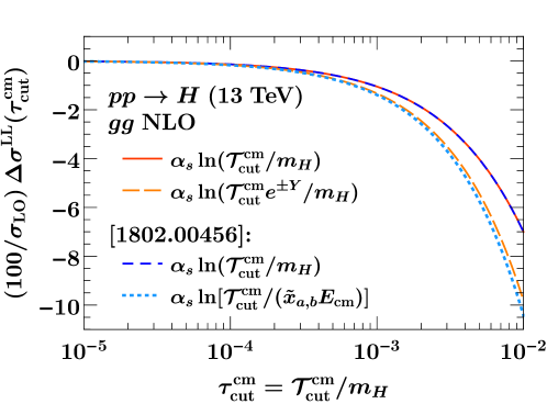
Figure 1: Comparison of the $Y$-integrated LL power correction for hadronic $\mathcal{T}$ for $gg\to Hg$. The solid red and blue dashed curves show the LL results keeping only $\ln(\mathcal{T}/m_{H})$. In the long-dashed orange and dotted light blue curves we keep all $\ln(\mathcal{T}e^{\pm Y}/m_{H})$ or $\ln[\mathcal{T}/(\tilde{x}_{a,b}E_{\mathrm{cm}})]$ terms. In both cases, our result in eq. (6.2.1) and the result of ref. Boughezal:2018mvf in eq. (123) agree. The small difference in the second case arises due to the fact that $e^{\pm Y}/m_{H}$ is not exactly the same as $\tilde{x}_{a,b}E_{\mathrm{cm}}$.

To illustrate this numerically, the $Y$-integrated results are compared in fig. 1. First note that the hadronic LL results in eq. (6.2.1) do not exactly correspond to those previously given in refs. Moult:2016fqy ; Moult:2017jsg . This is due to the formally NLL terms proportional to $\ln(\rho/e^{Y})$, discussed below eq. (6.2.1), which are dropped in the strict LL results in refs. Moult:2016fqy ; Moult:2017jsg , but are kept in eq. (6.2.1). The analogous NLL terms proportional to $\ln(\tilde{x}_{a,b}E_{\mathrm{cm}})$ are also kept in refs. Boughezal:2016zws ; Boughezal:2018mvf and eq. (123). Dropping these NLL terms in eqs. (123) and (6.2.1), our and their LL results defined in terms of the same $\ln(\mathcal{T}/m_{H})$ agree exactly, as shown by the solid red and blue dashed curves in fig. 1. The long-dashed orange and dotted blue curves in fig. 1 show the results when using instead $\ln(\mathcal{T}e^{\pm Y}/m_{H})$ or $\ln[\mathcal{T}/(\tilde{x}_{a,b}E_{\mathrm{cm}})]$ to multiply the LL coefficients. The observed difference to the solid red/dashed blue strict LL result has the size of a typical NLL contribution. There is also a very small difference between the long-dashed orange and dotted blue results due to the fact that $e^{\pm Y}/m_{H}$ is not exactly the same as $\tilde{x}_{a,b}E_{\mathrm{cm}}$. This difference is exactly accounted for by the last line in eq. (126).

6.2.2 Comparison at NLL

We now extend our comparison of the $Y$-integrated results to NLL, focusing again only on the $gg\to Hg$ channel, which contains all possible complications. The full NLL result of ref. Boughezal:2018mvf can be written as

$$\frac{\mathrm{d}\sigma^{\text{NLP\cite[cite]{\@@bibref{Authors Phrase1YearPhrase2}{Boughezal:2018mvf}{\@@citephrase{(}}{\@@citephrase{)}}}}}}{\mathrm{d}\mathcal{T}^{\mathrm{cm}}} =\frac{\alpha_{s}C_{A}}{\pi}\int_{0}^{1}\mathrm{d}\tilde{x}_{a}\mathrm{d}\tilde{x}_{b}\,2\pi\delta(\tilde{x}_{a}\tilde{x}_{b}E_{\mathrm{cm}}^{2}-m_{H}^{2})\frac{|{\mathcal{M}}^{\mathrm{LO}}_{gg\to H}(m_{H})|^{2}}{2\tilde{x}_{a}\tilde{x}_{b}E_{\mathrm{cm}}^{2}}\int_{\tilde{x}_{a}}^{1}\frac{\mathrm{d}z_{a}}{z_{a}}\frac{\tilde{x}_{a}E_{\mathrm{cm}}}{m_{H}^{2}}$$

$$\quad\times\biggl{\{}f_{g}\biggl{(}\frac{\tilde{x}_{a}}{z_{a}}\biggr{)}f_{g}(\tilde{x}_{b})\biggl{[}\biggl{(}\frac{(1-z_{a}+z_{a}^{2})^{2}}{z_{a}^{2}}-1\biggr{)}{\mathcal{L}}_{0}(1-z_{a})+\frac{3z_{a}^{2}+1-z_{a}+z_{a}^{3}}{z_{a}^{2}}\biggr{]}$$

$$\hskip 28.45274pt+\frac{\tilde{x}_{a}}{z_{a}}f^{\prime}_{g}\biggl{(}\frac{\tilde{x}_{a}}{z_{a}}\biggr{)}f_{g}(\tilde{x}_{b})\biggl{[}-\delta(1-z_{a})\ln\frac{\mathcal{T}^{\mathrm{cm}}}{\tilde{x}_{a}E_{\mathrm{cm}}}+\frac{(1-z_{a}+z_{a}^{2})^{2}}{z_{a}^{2}}{\mathcal{L}}_{0}(1-z_{a})\biggr{]}$$

$$\hskip 28.45274pt-f_{g}\biggl{(}\frac{\tilde{x}_{a}}{z_{a}}\biggr{)}\,\tilde{x}_{b}f^{\prime}_{g}(\tilde{x}_{b})\delta(1-z_{a})\biggr{\}}$$

$$\quad+(a\leftrightarrow b)\,.$$ (127)

To bring our result into this same form, we need to integrate by parts twice, first with respect to $Y$ as shown in eq. (6.2), and then with respect to $z_{a}$. The details of this calculation are given in appendix B. The final result is shown in eq. (B) and is given by the result of ref. Boughezal:2018mvf in eq. (6.2.2) plus an extra contribution,

$$\frac{\mathrm{d}\sigma^{(2,1)}}{\mathrm{d}\mathcal{T}^{\mathrm{cm}}} =\frac{\mathrm{d}\sigma^{\text{NLP\cite[cite]{\@@bibref{Authors Phrase1YearPhrase2}{Boughezal:2018mvf}{\@@citephrase{(}}{\@@citephrase{)}}}}}}{\mathrm{d}\mathcal{T}^{\mathrm{cm}}}$$ (128)

$$\quad+2\frac{\alpha_{s}C_{A}}{\pi}\int_{0}^{1}\mathrm{d}x_{a}\mathrm{d}x_{b}\,2\pi\delta(x_{a}x_{b}E_{\mathrm{cm}}^{2}-m_{H}^{2})\frac{|{\mathcal{M}}_{gg\to H}^{\mathrm{LO}}(m_{H})|^{2}}{2x_{a}x_{b}E_{\mathrm{cm}}^{2}}f_{g}(x_{a})f_{g}(x_{b})\,\frac{e^{Y}+e^{-Y}}{m_{H}}\,.$$

The two results should agree exactly upon integration, and we have not been able to find a source for this discrepancy. As discussed in more detail in sec. 7, the numerical comparison with MCFM provides a strong confirmation of our result. The numerical extraction of the integrated NLL coefficient yields $-0.460\pm 0.026$, which agrees well with our analytic predicted value of $-0.466$ (see table 2 below). Dropping the term in the final line of eq. (128) would instead predict the value $-1.669$.

7 Numerical Results

In this section we study our results numerically, including the size of the power corrections and the rapidity dependence. We also compare our analytic results for the ${\mathcal{O}}(\alpha_{s})$ NLP power corrections with the full nonsingular spectrum obtained numerically from the LO $V+$jet and $H+$jet calculations in MCFM8 Campbell:1999ah ; Campbell:2010ff ; Campbell:2015qma ; Boughezal:2016wmq . In refs. Moult:2016fqy ; Moult:2017jsg , the NLP corrections were extracted numerically by using a fit of the known form of their logarithmic structure to the nonsingular spectrum from MCFM8. In refs. Moult:2016fqy ; Moult:2017jsg , these fits were carried out for the leptonic definition. Here, we have in addition performed the fits also for the hadronic definition. We find excellent agreement between the analytically predicted values and the numerically extracted values for all coefficients, i.e., for the LL and NLL coefficients in all partonic channels for both the leptonic and hadronic definition. This provides a strong and independent cross check for the correctness of the analytic NLL results obtained here. By comparing the complete nonsingular spectrum with our NLP result, we can also assess the importance of power corrections beyond NLP.

The NLO power corrections for each partonic channel are extracted from the nonsingular spectrum by using the fit function

$$F_{\mathrm{NLO}}(\tau) =\frac{\mathrm{d}}{\mathrm{d}\ln\tau}\Bigl{\{}\tau\bigl{[}(a_{1}+b_{1}\tau+c_{1}\tau^{2})\ln\tau+a_{0}+b_{0}\tau+c_{0}\tau^{2}\bigr{]}\Bigr{\}}\,,$$ (129)

with $\tau\equiv\mathcal{T}_{0}/m_{Z}$ for $Z$ production and $\tau\equiv\mathcal{T}_{0}/m_{H}$ for Higgs production. Details of the fitting procedure have been described already in refs. Moult:2016fqy ; Moult:2017jsg , so we do not repeat them here. A key point is that in order to obtain a precise and unbiased fit result for the to-be extracted $a_{i}$ coefficients, it is crucial to include the higher-power $b_{i}$ and $c_{i}$ terms in eq. (129), and to carefully choose the fit range and verify the stability of the fit, as was done in refs. Moult:2016fqy ; Moult:2017jsg . At the level of precision the $a_{i}$ are extracted, this is essential since the full nonsingular cross section includes the complete set of power corrections and if the $b_{i}$ and $c_{i}$ terms were neglected, these higher-power corrections would be absorbed by the $a_{i}$ terms in the fit, rendering their numerically extracted values meaningless. To obtain a precise extraction of the NLL coefficient $a_{0}$, we fix the LL coefficient $a_{1}$ in the fit to its analytic result.

The relevant coefficients for our NLP comparison at NLO are the LL coefficient $a_{1}$ and the NLL coefficient $a_{0}$. For leptonic $\mathcal{T}$ they were extracted for Drell-Yan in ref. Moult:2016fqy and for gluon-fusion Higgs in ref. Moult:2017jsg and for the hadronic $\mathcal{T}$ we have obtained them here. Depending on the partonic channel, the uncertainties on the fitted coefficients range from $0.08\%$ to $2.3\%$ for leptonic $\mathcal{T}$ and from $0.6\%$ to $5.7\%$ for hadronic $\mathcal{T}$. The latter has larger uncertainties because its power corrections are larger, requiring the fit to be restricted to smaller $\mathcal{T}$ values where the uncertainties in the nonsingular data are larger.

7.1 Drell-Yan Production

We first consider Drell-Yan production, taking $pp\to Z/\gamma^{*}$ at $E_{\rm cm}=13\,\mathrm{TeV}$. We use the MMHT2014 NNLO PDFs Harland-Lang:2014zoa with fixed scales $\mu_{r}=\mu_{f}=m_{Z}$, and $\alpha_{s}(m_{Z})=0.118$. We fix $Q=m_{Z}$, integrate over the vector-boson rapidity, and work in the narrow-width approximation for the $Z$-boson. The NLP corrections for the leptonic $\mathcal{T}$ definition were numerically extracted in ref. Moult:2016fqy . The results for both the leptonic and hadronic definitions for all partonic channels are collected and compared to our analytic predictions in table 1. We find excellent agreement within the fit uncertainties in all cases.

NLO $\mathcal{T}_{0}^{\rm lep}$ $q\bar{q}\to Zg$	$a_{1}$	$a_{0}$
fitted Moult:2016fqy	$+0.25366\pm 0.00131$	$+0.13738\pm 0.00057$
analytic	$+0.25509$	$+0.13708$
NLO $\mathcal{T}_{0}^{\rm lep}$ $qg+gq\to Zq$	$a_{1}$	$a_{0}$
fitted Moult:2016fqy	$-0.27697\pm 0.00113$	$-0.40062\pm 0.00052$
analytic	$-0.27720$	$-0.40105$
NLO $\mathcal{T}_{0}^{\mathrm{cm}}$ $q\bar{q}\to Zg$	$a_{1}$	$a_{0}$
fitted	$+1.4188\pm 0.0614$	$-2.4808\pm 0.0176$
analytic	$+1.3935$	$-2.4806$
NLO $\mathcal{T}_{0}^{\mathrm{cm}}$ $qg+gq\to Zq$	$a_{1}$	$a_{0}$
fitted	$-2.2981\pm 0.0442$	$+4.0991\pm 0.0132$
analytic	$-2.3224$	$+4.0965$

Table 1: Comparison between our analytic predictions and the fitted results for the LL $a_{1}$ and NLL $a_{0}$ coefficients in Drell-Yan production. These fitted values for $a_{1}$ and $a_{0}$ with the leptonic definition and the analytic results for $a_{1}$ were already given in ref. Moult:2016fqy .

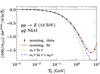
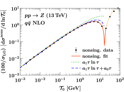
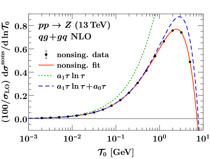
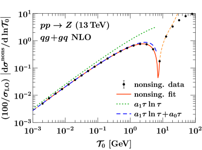
Figure 2: The ${\mathcal{O}}(\alpha_{s})$ nonsingular corrections for $Z$ production for the $q\bar{q}$ channel (top row) and the $qg+gq$ channel (bottom row). A fit to the nonsingular data is shown by the solid red curve. The LL and NLL results are shown by green dotted and blue dashed curves, respectively. In all cases, the NLL approximation provides an excellent approximation to the complete nonsingular cross section.

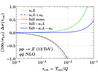
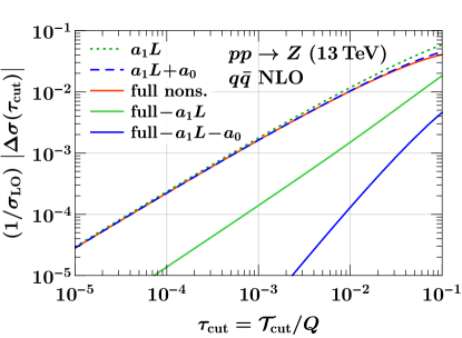
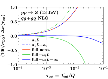
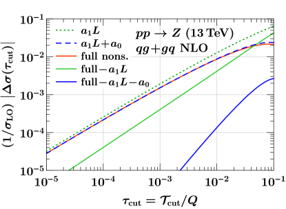
Figure 3: The power corrections for the cumulative $\Delta\sigma(\tau_{\mathrm{cut}})$ at ${\mathcal{O}}(\alpha_{s})$ for $Z$ production in the $q\bar{q}$ channel (top row) and $qg+gq$ channel (bottom row). In both cases, after the inclusion of the NLL power corrections, $\Delta\sigma(\tau_{\mathrm{cut}})$ is reduced by a factor of 100 or more for $\tau_{\mathrm{cut}}<10^{-2}$.

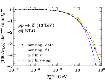
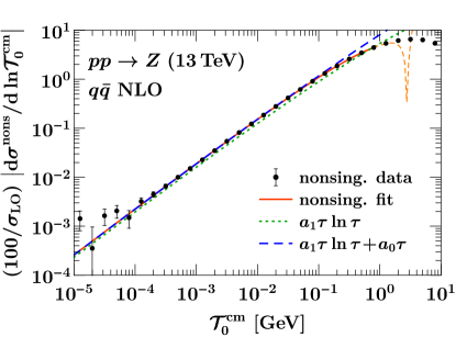
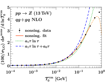
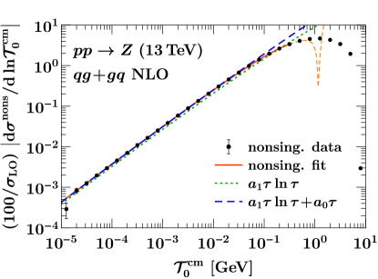
Figure 4: Same as fig. 2 for the hadronic $\mathcal{T}$ definition.

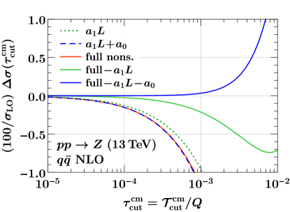
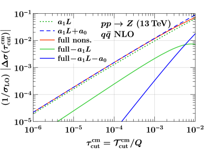
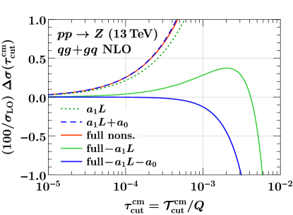
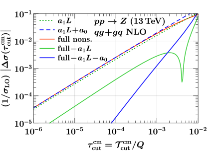
Figure 5: Same as fig. 3 for the hadronic $\mathcal{T}$ definition.

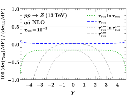
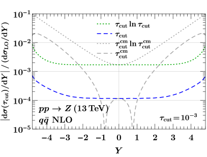
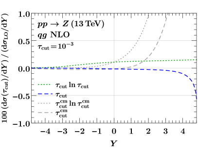
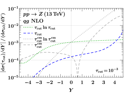
Figure 6: The NLO NLP corrections as a function of rapidity at fixed $\tau_{\mathrm{cut}}=10^{-3}$ for $Z$ production for the $q\bar{q}$ channel (top row) and the $qg$ channel (bottom row). The LL and NLL coefficients for leptonic $\mathcal{T}$ are shown by the green dotted and blue dashed curves and for hadronic $\mathcal{T}$ by the dotted and dashed gray curves.

In fig. 2 we show the complete NLO nonsingular contributions as black dots, as well as a fit to their form with the solid red curve. Given the agreement in table 1 between our analytic $a_{0}$ and the earlier fit result for $a_{0}$, we have fixed $a_{0}$ to the analytic result, and redone the fit using eq. (129) to obtain this red curve. The red curve from this fit is fully consistent with the earlier fit result from ref. Moult:2016fqy . The dashed orange curve in fig. 2 is the extension of the fit function beyond its fit range. In dotted green and dashed blue we show our analytic predictions. We see that with the inclusion of the NLL power corrections, we obtain an excellent description of the full nonsingular cross section up to nearly $\mathcal{T}_{0}\sim 1$ GeV. This is quite remarkable, and shows that additional higher-order power correction terms are truly suppressed.

In fig. 3 we show a plot of the corresponding residual power corrections for the cumulant, $\Delta\sigma(\tau_{\mathrm{cut}})$, on both a linear scale (left) and logarithm scale (right). The solid red curve shows the full power corrections, the solid green curves show the remaining power corrections after including $a_{1}$ in the subtractions, and the solid blue curve those after including $a_{1}$ and $a_{0}$ in the subtractions. We see that with the inclusion of the full NLL power corrections, we achieve more than a factor of $100$ reduction in the residual power corrections as compared with the leading-power result at NLO. Both partonic channels have similarly sized power corrections and show a fast convergence of the power expansion. The fact that the blue curve in the logarithmic plot exhibits a steeper slope than the red and green curves is due to its $\mathcal{O}(\tau_{\mathrm{cut}}^{2})$ scaling corresponding to a next-to-next-to-leading power correction. This provides a nice visualization that our results correctly capture the complete NLP contribution.

The analogous results for the fitted nonsingular spectrum and the residual power corrections $\Delta\sigma(\tau^{\mathrm{cm}}_{\mathrm{cut}})$ for the hadronic $\mathcal{T}$ definition are shown in figs. 4 and 5. As expected, the power corrections are substantially larger for $\mathcal{T}^{\mathrm{cm}}$ than for the leptonic definition. To obtain similarly sized power corrections, one has to go to about an order of magnitude smaller values of $\mathcal{T}^{\mathrm{cm}}$. Apart from the overall enhancement, the qualitative behavior of the LL and NLL contributions and the different partonic channels is the same. This is expected from our analytic results, which show that the coefficients for both definitions have essentially the same structure and primarily differ in the overall factors of $e^{\pm Y}$ leading to the rapidity enhancement for the hadronic definition already observed in refs. Moult:2016fqy ; Moult:2017jsg .

In fig. 6 we show the rapidity dependence of the NLP corrections at fixed $\tau_{\mathrm{cut}}=10^{-3}$ for both leptonic and hadronic $\mathcal{T}$ normalized to the LO rapidity spectrum. We can clearly see the exponential enhancement for the hadronic definition at large $\lvert Y\rvert$. For the $qg$ channel, the asymmetric behavior in rapidity is expected from its analytic result. The result for the $gq$ channel corresponds to taking $Y\to-Y$, such that their sum is symmetric in rapidity. While the leptonic definition does not suffer from the exponential enhancement of the hadronic definition, it still exhibits a substantial increase at large positive $Y$ in the $qg$ channel, as well as a suppression at large negative $Y$. This is due to the substantially different $x$-dependence of the quark-gluon luminosity (and its derivative) compared to the $q\bar{q}$ luminosity in the LO result to which we normalize. Knowing the NLL contribution to the power corrections differential in rapidity enables one to explicitly account for this effect in the subtractions.

7.2 Gluon-Fusion Higgs Production

Next, we consider gluon-fusion Higgs production. We take $pp\to H$ at $E_{\rm cm}=13\,\mathrm{TeV}$ with an on-shell, stable Higgs boson with $m_{H}=125\,\mathrm{GeV}$, integrated over all $Y$. We use the MMHT2014 NNLO PDFs Harland-Lang:2014zoa , with fixed scales $\mu_{r}=\mu_{f}=m_{H}$, and $\alpha_{s}(m_{H})=0.1126428$. The NLP power corrections for this configuration for the leptonic $\mathcal{T}$ definition were extracted numerically in ref. Moult:2017jsg . The results for both leptonic and hadronic definitions for all partonic channels are collected and compared to our analytic predictions in table 2. In all cases, excellent agreement is observed within the fit uncertainties.

NLO $\mathcal{T}_{0}^{\rm lep}$ $gg\to Hg$	$a_{1}$	$a_{0}$
fitted Moult:2017jsg	$+0.60936\pm 0.00600$	$+0.18241\pm 0.00425$
analytic	$+0.60400$	$+0.18627$
NLO $\mathcal{T}_{0}^{\rm lep}$ $gq+qg\to Hq$	$a_{1}$	$a_{0}$
fitted Moult:2017jsg	$-0.03733\pm 0.00066$	$-0.42552\pm 0.00032$
analytic	$-0.03807$	$-0.42576$
NLO $\mathcal{T}_{0}^{\rm lep}$ $q\bar{q}\to Hg$	$a_{1}$	$10^{3}\,a_{0}$
fitted Moult:2017jsg	–	$+4.90060\pm 0.00013$
analytic	–	$+4.90047$
NLO $\mathcal{T}_{0}^{\mathrm{cm}}$ $gg\to Hg$	$a_{1}$	$a_{0}$
fitted	$+1.5436\pm 0.0585$	$-0.45954\pm 0.02606$
analytic	$+1.5225$	$-0.46646$
NLO $\mathcal{T}_{0}^{\mathrm{cm}}$ $gq+qg\to Hq$	$a_{1}$	$a_{0}$
fitted	$-0.06606\pm 0.00161$	$-0.33932\pm 0.00194$
analytic	$-0.06498$	$-0.34068$
NLO $\mathcal{T}_{0}^{\mathrm{cm}}$ $q\bar{q}\to Hg$	$a_{1}$	$10^{3}\,a_{0}$
fitted	–	$+6.13445\pm 0.00015$
analytic	–	$+6.13448$

Table 2: Comparison between our analytic predictions and the fitted results for the LL $a_{1}$ and NLL $a_{0}$ coefficients in Higgs production. These fitted values for $a_{1}$ and $a_{0}$ with the leptonic definition and the analytic results for $a_{1}$ were already given in ref. Moult:2017jsg .

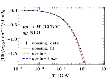
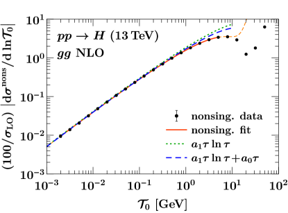
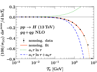
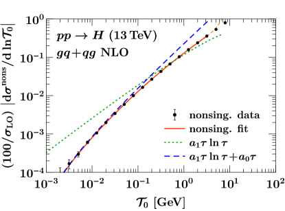
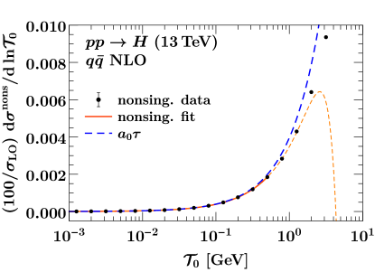
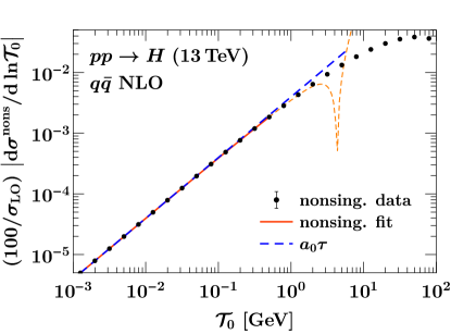
Figure 7: The ${\mathcal{O}}(\alpha_{s})$ nonsingular corrections for Higgs production for the $gg$ channel (top row), $gq+qg$ channel (middle row), and $q\bar{q}$ channel (bottom row). A fit to the nonsingular data (black dots) is shown by the solid red curve. The LL and NLL results are shown by green dotted and blue dashed curves, respectively. In all cases, the NLL approximation provides an excellent approximation to the complete nonsingular cross section for sufficiently small $\mathcal{T}_{0}$.

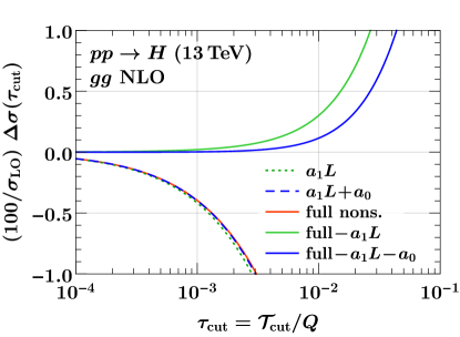
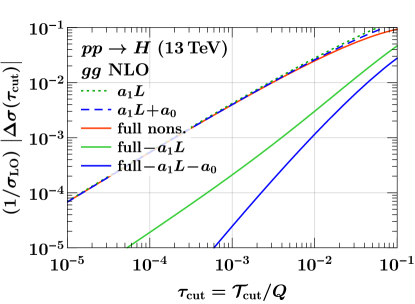
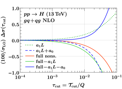
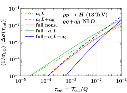
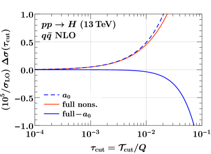
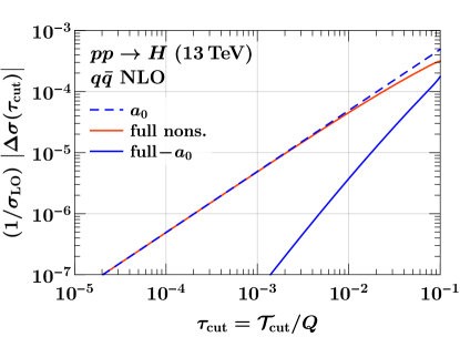
Figure 8: The power corrections for the cumulant $\Delta\sigma(\tau_{\mathrm{cut}})$ at ${\mathcal{O}}(\alpha_{s})$ for Higgs production in the $gg$ channel (top row), $gq+qg$ channel (middle row), $q\bar{q}$ channel (bottom row).

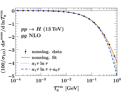
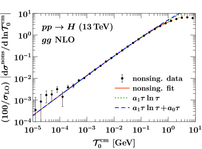
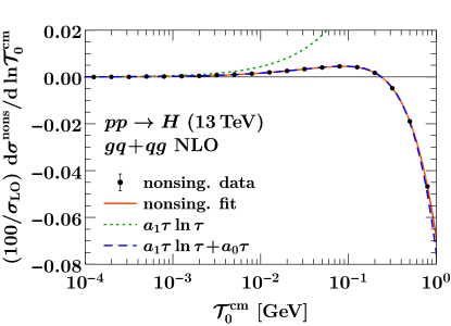
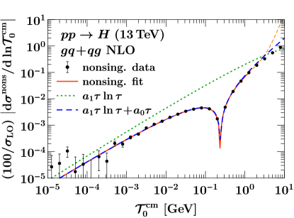
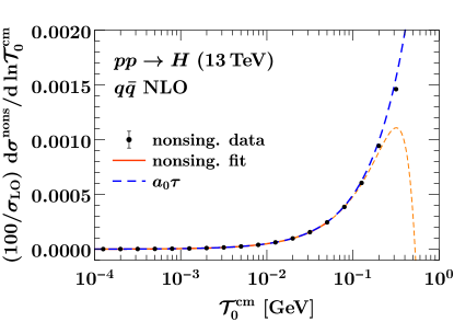
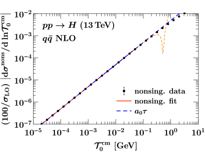
Figure 9: Same as fig. 7 for the hadronic $\mathcal{T}$ definition.

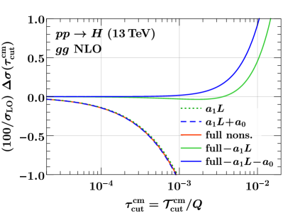
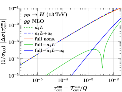
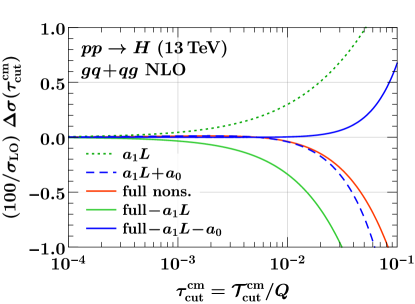
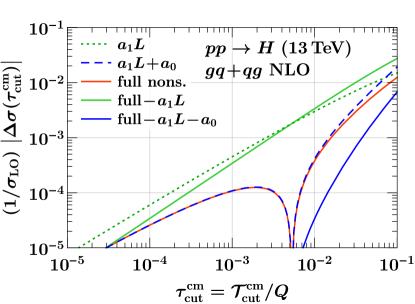
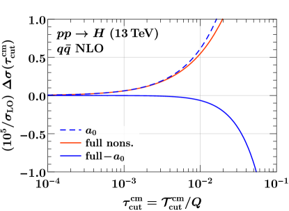
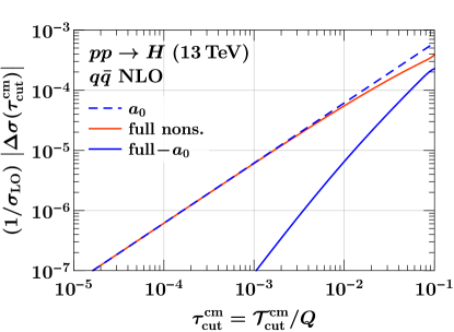
Figure 10: Same as fig. 8 for the hadronic $\mathcal{T}$ definition.

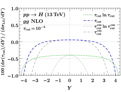
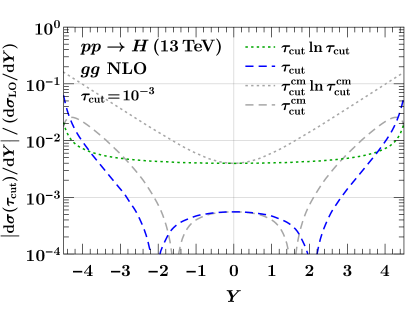
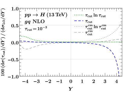
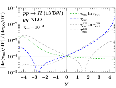
Figure 11: The NLO NLP corrections as a function of rapidity at fixed $\tau_{\mathrm{cut}}=10^{-3}$ for Higgs production for the $gg$ channel (top row) and the $gq$ channel (bottom row). The LL and NLL coefficients for leptonic $\mathcal{T}$ are shown by the green dotted and blue dashed curves and for hadronic $\mathcal{T}$ by the dotted and dashed gray curves.

In fig. 7 we show as the solid red curve a fit to the full nonsingular result at NLO (black points), which is compared with the LL and NLL predictions in dashed green and dashed blue, respectively. Once again this solid red fit curve is obtained using the form in eq. (129) with $a_{1}$ and $a_{0}$ fixed by the analytic result in table 2, and agrees very well with the corresponding result obtained in ref. Moult:2017jsg where $a_{0}$ was a parameter in the fit. In all cases, we find that the NLL result provides a good description of the full nonsingular cross section. This is expected since the NLL results includes all NLP terms in the NLO cross section. We see, however, that particularly for the $gq+qg$ channel, the NLL result for $a_{0}$ is required to get a good description, and the LL power correction $a_{1}$ alone is not sufficient. Thus the $gq+qg$ channel provides an example where simply looking at the size of the residual nonsingular result after subtracting the $a_{1}$ term does not suffice to validate the value of this coefficient.

In fig. 8, we show a plot of the corresponding power corrections for the cumulant, $\Delta\sigma(\tau_{\mathrm{cut}})$, on both a linear scale (left) and logarithm scale (right). Here we more easily see that the inclusion of the NLL power corrections significantly reduces the residual power corrections for the subtractions. For the dominant $gg\to Hg$ channel at a typical value of $\tau_{\mathrm{cut}}\sim 10^{-3}$ approximately one order of magnitude is gained at each logarithmic order that the power corrections are computed. From table 2, we see that for the $gq+qg\to Hq$ channel, the LL coefficient is numerically suppressed, while in contrast its NLL coefficient is quite larger. Due to this unusual behavior, the NLL result is required to consistently reduce the power corrections as compared with the leading-power result. In the $q\bar{q}$ channel there is no $a_{1}$ term, and significant improvement is apparent from including $a_{0}$.

The analogous results for the fitted nonsingular spectrum and the residual power corrections $\Delta\sigma(\tau^{\mathrm{cm}}_{\mathrm{cut}})$ for the hadronic $\mathcal{T}$ definition are shown in figs. 9 and 10. The power corrections are noticeably larger, though the effect of the rapidity enhancement is not as pronounced as for Drell-Yan, since here the PDFs suppress the cross section contributions at larger rapidities. For the dominant $gg\to Hg$ channel there are also numerical cancellations in the NLL coefficient. More precisely the value for $a_{0}$ in table 2 arises as $a_{0}=2.356+(-2.822)=-0.466$, where the first term corresponds to the rapidity-enhanced version of the leptonic $a_{0}$ while the second term is the NLL contribution arising from the additional rapidity dependence in the argument of the leading logarithm discussed below eq. (6.2.1). As a result of this cancellation, including only $a_{1}$ in the subtractions leads to slightly smaller power correction above $\tau_{\mathrm{cut}}>10^{-3}$ than subtracting both $a_{1}$ and $a_{0}$ (compare the green and blue solid lines in the top row of fig. 10). If the second NLL contribution were included as part of the LL result, the latter would provide a much poorer approximation and including the remaining NLL contribution would provide a substantial improvement. Either way, the remaining power corrections after subtracting the full NLL result shows a much steeper slope, which is as expected from its $\mathcal{O}(\tau_{\mathrm{cut}}^{2})$ scaling. This provides another example where considering only the overall size of the improvement can be potentially misleading. The $gq+qg\to Hq$ channel shows a similarly unusual behavior as for the leptonic definition.

In fig. 11 we show the rapidity dependence of the NLP corrections at fixed $\tau_{\mathrm{cut}}=10^{-3}$ for both leptonic and hadronic $\mathcal{T}$ normalized to the LO rapidity spectrum. The exponential enhancement for the hadronic definition at large $\lvert Y\rvert$ is again apparent in the LL results. The NLL coefficients again exhibit an enhancement already for the leptonic definition at large $Y$. This is again due to the different $x$ dependence of the quark PDF and the PDF derivatives compared to the LO $gg$ luminosity to which we normalize. The quark PDF contributions are also the main reason why the NLL term for the $gq$ channel ($a_{0}$ in table 2) is much larger than the LL contribution. For the hadronic definition, the $e^{\pm Y}$ factors from the observable definition turn out to partially compensate these PDF effects. This is best visible in the $gq$ channel, where the PDF enhanced terms at negative (LL) or positive (NLL) $Y$ get reduced by a $e^{\pm Y}$ factor from the observable definition. The same effect is also present in the $gg$ channel at NLL. This is the reason why the $a_{0}$ term for the hadronic definition in the $gq$ channel turns out to be even slightly smaller than for the leptonic definition.

8 Conclusions

In this paper, we have computed the next-to-leading power corrections in the $N$-jettiness resolution variable for Drell-Yan and gluon-fusion Higgs production at NLO. This builds on our previous work by computing the non-logarithmically enhanced terms at this order. These results enable the performance of the $N$-jettiness subtraction method to be improved, and provide important information on the structure of subleading power corrections beyond the leading logarithms. Our calculation is based on a master formula applicable to $\text{SCET}_{\text{I}}$ observables, and highlights a large degree of universality of these power corrections.

We explained in detail the issue of the treatment of Born measurements at subleading power. We have shown that an apparent disagreement in the literature arises due to the fact that the representation used to obtain the power corrections in refs. Boughezal:2016zws ; Boughezal:2018mvf is only valid when integrated over all rapidities, and therefore cannot be directly compared with the results of refs. Moult:2016fqy ; Moult:2017jsg and those in the present paper, which are differential in rapidity. We show that after integration over rapidity the LL results agree. Further details can be found in sec. 6.

We find that the rapidity dependence of the NLL terms is quite sizeable and is therefore important to know to be able to improve the subtractions. One reason for this effect is the different $x$-dependence of parton luminosities or derivatives of PDFs appearing in the power corrections as compared to the Born-level parton luminosity. Hence, one can expect this to be a generic feature of subleading power corrections.

We also compared our analytic NLL results for gluon fusion Higgs production and Drell-Yan to numerical predictions for these NLO power corrections obtained from a fit to data from MCFM. In all cases, excellent agreement was found. In addition we studied the extent to which the inclusion of the NLL power corrections improves the subtraction. At NLO, the inclusion of the NLL power corrections completely captures the ${\mathcal{O}}(\tau)$ terms. Numerically, summing over production channels, the inclusion of these results reduces the size of the power corrections by two orders of magnitude in Higgs production and three orders of magnitude in Drell-Yan production.

There are a number of directions for future work. It will be interesting to extend the calculation of the NLL power corrections to NNLO. Generically we expect up to an order of magnitude improvement could also be obtained by extending the known LL power corrections at this order to NLL. Beyond fixed order, the derivation of subleading power renormalization group evolution equations at NLL would allow for the all-orders prediction of the NLL terms. Finally, while we have focused here on color-singlet production, our results provide an important step toward the calculation of the NLP corrections at higher orders and for more complicated processes.

Appendix A Derivation of NLO Leading Power Results

At leading power the singular terms for $N$-jettiness are most easily obtained from known factorization formulas Stewart:2009yx ; Stewart:2010tn , which describe the singular behavior of the observable to all orders. The fixed order approach of this paper is therefore most useful when such factorization formula are not available, or well understood, such as at subleading power. However, it can also be applied to reproduce the LP results. In this appendix we illustrate this at NLO, by reproducing the one-loop beam and soft functions for beam thrust.

To relate the beam and soft functions as defined in SCET to our calculation in this work, recall the LP factorization formula for beam thrust Stewart:2009yx ,

$$\frac{\mathrm{d}\sigma^{(0)}}{\mathrm{d}Q^{2}\mathrm{d}Y\mathrm{d}\mathcal{T}}=\hat{\sigma}^{\mathrm{LO}}(Q,Y)\,H_{ab}(Q,\mu)\int\mathrm{d}t_{a}\mathrm{d}t_{b}\,B_{a}(t_{a},x_{a},\mu)B_{b}(t_{b},x_{b},\mu)S\biggr{(}\mathcal{T}-\frac{t_{a}}{Q}-\frac{t_{b}}{Q},\mu\biggr{)}\,,$$ (130)

where the superscript ⁽⁰⁾ refers to LP, and as before $x_{a,b}=\frac{Q}{E_{\mathrm{cm}}}e^{\pm Y}$. The hard function $H_{ab}$ describes virtual corrections to the hard process $ab\to L$, $B_{a,b}$ are the two beam functions and $S$ is the soft function. The beam functions can be further matched onto normal PDFs,

$$B_{i}(t,x,\mu)=\sum_{j}\int_{x}^{1}\frac{\mathrm{d}z}{z}{\mathcal{I}}_{ij}(t,z,\mu)f_{j}\biggl{(}\frac{x}{z},\mu\biggr{)}\,.$$ (131)

All of these functions have definitions as field theory matrix elements in the EFT. Their fixed order definitions give rise to UV divergences, which are as usual removed by a renormalization procedure, which in turn gives rise to RGEs that can be used to resum large logarithms of $\mathcal{T}$. In the approach presented in this paper, the same divergences appear as $1/\epsilon$ IR divergences in the soft and collinear limits of QCD amplitudes.

At LO, we have

$$H^{\mathrm{LO}}_{ij}(Q^{2},\mu)=1\,,\quad{\mathcal{I}}_{ij}^{\mathrm{LO}}(t,x,\mu)=\delta_{ij}\delta(t)\,,\quad S^{\mathrm{LO}}(\mathcal{T},\mu)=\delta(\mathcal{T})\,.$$ (132)

At one loop, the convolution structure thus becomes trivial. Working with hard, beam, soft, and PDFs in the bare factorization theorem we have

$$\frac{\mathrm{d}\sigma^{(0,1)}}{\mathrm{d}Q^{2}\mathrm{d}Y\mathrm{d}\mathcal{T}} =\hat{\sigma}^{\mathrm{LO}}\,H^{\mathrm{NLO}}_{ab}(Q^{2},\epsilon)\delta(\mathcal{T})f_{a}(x_{a},\epsilon)f_{b}(x_{b},\epsilon)$$

$$+\hat{\sigma}^{\mathrm{LO}}\sum_{a^{\prime}}\int_{x_{a}}^{1}\frac{\mathrm{d}z_{a}}{z_{a}}\,Q\,{\mathcal{I}}^{\mathrm{NLO}}_{aa^{\prime}}(Q\mathcal{T},z_{a},\epsilon)f_{a^{\prime}}(x_{a}/z_{a},\epsilon)f_{b}(x_{b},\epsilon)$$

$$+\hat{\sigma}^{\mathrm{LO}}\sum_{b^{\prime}}\int_{x_{b}}^{1}\frac{\mathrm{d}z_{b}}{z_{b}}\,Q\,{\mathcal{I}}^{\mathrm{NLO}}_{bb^{\prime}}(Q\mathcal{T},z_{b},\epsilon)f_{a}(x_{a},\epsilon)f_{b^{\prime}}(x_{b}/z_{b},\epsilon)$$

$$+\hat{\sigma}^{\mathrm{LO}}f_{a}(x_{a},\epsilon)f_{b}(x_{b},\epsilon)S^{\mathrm{NLO}}(\mathcal{T},\epsilon)\,.$$ (133)

Note the extra factor of $Q$ in the beam contributions, arising from $t_{a,b}$ and $\mathcal{T}$ having different mass dimensions. We have written eq. (A) in a form similar to our master formulas, such that we can easily read off the one-loop beam function kernels and soft function. The $\epsilon$ arguments in eq. (A) all refer to ultraviolet divergences and can be removed by SCET counterterms to obtain the renormalized factorization theorem. To obtain this it is important to include virtual graphs in the various sectors as well as zero-bin subtractions for the beam functions.

A.1 Leading-Power Expansion of Matrix Elements

The leading-power behavior of real emission matrix elements in the soft and collinear limits is universal, see e.g. Catani:1996vz , and has already been used in sec. 4.4. Here, we briefly review the relevant formulas, and give the relevant one-loop expressions.

Given the Born process

$$\kappa_{a}(q_{a})+\kappa_{b}(q_{b})\to L(q_{a}+q_{b})\,,$$ (134)

where the incoming momenta are given by

$$q_{a}^{\mu}=Qe^{Y}\frac{n^{\mu}}{2}\,,\quad q_{b}^{\mu}=Qe^{-Y}\frac{\bar{n}^{\mu}}{2}\,,$$ (135)

and we write the one-emission process as

$$\kappa^{\prime}_{a}(q^{\prime}_{a})+\kappa^{\prime}_{b}(q^{\prime}_{b})\to L(q^{\prime}_{a}+q^{\prime}_{b}-k)+\kappa_{1}(k)\,.$$ (136)

In the soft limit $k^{\mu}\ll q_{a}^{\mu},q_{b}^{\mu}$, the squared matrix element obeys the LP relation

$$A^{(0)}_{a^{\prime}b^{\prime}\to Lk}(Q,Y;\{k\}) =\frac{16\pi\alpha_{s}\mu_{\rm MS}^{2\epsilon}\mathbf{C}}{k^{+}k^{-}}\times\delta_{aa^{\prime}}\,\delta_{bb^{\prime}}\,A^{\mathrm{LO}}_{ab\to L}(Q,Y)\,,$$ (137)

where we made explicit that a soft emission can not change the incoming flavors. $\mathbf{C}=C_{F},C_{A}$ is the Casimir constant for $ab=q\bar{q},gg$.

In the LP $n$-collinear limit, the particle $k$ arises from the splitting $\kappa^{\prime}_{a}\to\kappa_{a}+\kappa_{1}$. If this splitting is allowed, at LP we have (in the notation of sec. 4) $q^{\prime}_{a}=q_{a}/z_{a}$ and $q^{\prime}_{b}=q_{b}$, and the LP limit of the matrix element is given by

$$A^{(0)}_{a^{\prime}b^{\prime}\to Lk}(Q,Y,\{k\})=\frac{8\pi\alpha_{s}\mu_{\rm MS}^{2\epsilon}}{Qe^{Y}k^{+}}P_{aa^{\prime}}(z_{a},\epsilon)\times\delta_{bb^{\prime}}\,A_{ab\to L}^{\mathrm{LO}}(Q,Y)\,.$$ (138)

Similarly, in the $\bar{n}$-collinear limit arising from $\kappa^{\prime}_{b}\to\kappa_{b}+\kappa_{1}$, at LP we get $q^{\prime}_{a}=q_{a},q^{\prime}_{b}=q_{b}/z_{b}$,

$$A^{(0)}_{a^{\prime}b^{\prime}\to Lk}(Q,Y,\{k\})=\frac{8\pi\alpha_{s}\mu_{\rm MS}^{2\epsilon}}{Qe^{-Y}k^{-}}P_{bb^{\prime}}(z_{b},\epsilon)\times\delta_{aa^{\prime}}\,A_{ab\to L}^{\mathrm{LO}}(Q,Y)\,.$$ (139)

The one-loop splitting functions in $d=4-2\epsilon$ dimensions are given by Catani:1996vz

$$P_{qq}(z,\epsilon) =C_{F}\biggl{[}\frac{1+z^{2}}{1-z}-\epsilon(1-z)\biggr{]}\,,$$

$$P_{gq}(z,\epsilon) =C_{F}\biggl{[}\frac{1+(1-z)^{2}}{z}-\epsilon z\biggr{]}\,,$$

$$P_{qg}(z,\epsilon) =T_{F}\biggl{[}1-\frac{2z(1-z)}{1-\epsilon}\biggr{]}\,,$$

$$P_{gg}(z,\epsilon) =2C_{A}\biggl{[}\frac{z}{1-z}+\frac{1-z}{z}+z(1-z)\biggr{]}\,.$$ (140)

Note that we flipped the notation of $qg$ and $gq$ relative to Catani:1996vz , following the standard convention.

A.2 NLO Soft Function

The NLO LP soft function follows from combining eq. (37) with eq. (137) using the same steps as in sec. 4.3,

$$\frac{\mathrm{d}\sigma_{s}^{(0,1)}}{\mathrm{d}Q^{2}\mathrm{d}Y\mathrm{d}\mathcal{T}} =\int_{0}^{\infty}\frac{\mathrm{d}k^{+}\mathrm{d}k^{-}}{(k^{+}k^{-})^{\epsilon}}\frac{f_{a}(x_{a})f_{b}(x_{b})}{(4\pi)^{2}2x_{a}x_{b}E_{\mathrm{cm}}^{4}}\frac{(4\pi)^{\epsilon}}{\Gamma(1-\epsilon)}A^{(0)}(Q,Y;\{k\})\,\delta\bigl{[}\mathcal{T}-\hat{\mathcal{T}}(\{k\})\bigr{]}$$

$$=\frac{A^{\mathrm{LO}}(Q,Y)}{2x_{a}x_{b}E_{\mathrm{cm}}^{4}}\frac{\alpha_{s}\mathbf{C}}{\pi}f_{a}(x_{a})f_{b}(x_{b})\times\frac{e^{\epsilon\gamma_{E}}\mu^{2\epsilon}}{\Gamma(1-\epsilon)}\int_{0}^{\infty}\frac{\mathrm{d}k^{+}\mathrm{d}k^{-}}{(k^{+}k^{-})^{\epsilon+1}}\delta\bigl{[}\mathcal{T}-\hat{\mathcal{T}}(\{k\})\bigr{]}$$

$$=\hat{\sigma}^{\mathrm{LO}}(Q,Y)\frac{\alpha_{s}\mathbf{C}}{\pi}f_{a}(x_{a})f_{b}(x_{b})\frac{e^{\epsilon\gamma_{E}}}{\Gamma(1-\epsilon)}\frac{2}{\epsilon}\frac{1}{\mu}(\mathcal{T}/\mu)^{-1-2\epsilon}$$

$$=\hat{\sigma}^{\mathrm{LO}}(Q,Y)\frac{\alpha_{s}\mathbf{C}}{4\pi}f_{a}(x_{a})f_{b}(x_{b})\biggl{[}-\frac{4}{\epsilon^{2}}\delta(\mathcal{T})+\frac{8}{\epsilon}\frac{1}{\mu}{\mathcal{L}}_{0}(\mathcal{T}/\mu)$$

$$\hskip 147.95424pt-\frac{16}{\mu}{\mathcal{L}}_{1}(\mathcal{T}/\mu)+\frac{\pi^{2}}{3}\delta(\mathcal{T})+{\mathcal{O}}(\epsilon)\biggr{]}\,.$$ (141)

The ${\mathcal{L}}_{n}(x)$ are the standard one-dimensional plus distributions, see e.g. Ligeti:2008ac for details. Note that there, the precise definition of the $\overline{\text{MS}}$ scheme is important. We use

$$\mu^{2}\equiv\mu^{2}_{\overline{\rm MS}}=\frac{4\pi}{e^{\gamma_{E}}}\mu_{\rm MS}^{2}\,.$$ (142)

If one were to use $\mu^{2\epsilon}=\frac{(4\pi)^{\epsilon}}{\Gamma(1-\epsilon)}\mu_{\rm MS}^{2\epsilon}$, one would miss the $\pi^{2}/3$ term. For the NLP results presented in the main text, both definitions yield identical results.

Taking eq. (A.2) and adding the virtual soft diagram, and then comparing to eq. (A), the one-loop bare soft function can be read off as

$$S^{\mathrm{NLO}}(\mathcal{T},\epsilon)=\frac{\alpha_{s}\mathbf{C}}{4\pi}\biggl{[}-\frac{4}{\epsilon^{2}}\delta(\mathcal{T})+\frac{8}{\epsilon}\frac{1}{\mu}{\mathcal{L}}_{0}(\mathcal{T}/\mu)-\frac{16}{\mu}{\mathcal{L}}_{1}(\mathcal{T}/\mu)+\frac{\pi^{2}}{3}\delta(\mathcal{T})\biggr{]}\,.$$ (143)

The finite terms precisely yield the renormalized one-loop soft function Stewart:2009yx .

A.3 NLO Beam Function

Applying the LP master formula eq. (37) to the $n$-collinear case and following the same steps as in sec. 4.2 gives

$$\frac{\mathrm{d}\sigma_{n}^{(0,1)}}{\mathrm{d}Q^{2}\mathrm{d}Y\mathrm{d}\mathcal{T}} =\int_{x_{a}}^{1}\frac{\mathrm{d}z_{a}}{z_{a}}\,\frac{f_{a^{\prime}}(x_{a}/z_{a})f_{b}(x_{b})}{2x_{a}x_{b}E_{\mathrm{cm}}^{4}}\frac{Qe^{Y}}{\rho}\biggl{(}\frac{Q\mathcal{T}e^{Y}}{\rho}\biggr{)}^{-\epsilon}\frac{z_{a}^{\epsilon}}{(1-z_{a})^{\epsilon}}\frac{(4\pi)^{\epsilon}}{(4\pi)^{2}\Gamma(1-\epsilon)}$$

$$\hskip 42.67912pt\times A(Q,Y;\{k\})\,.$$ (144)

Using the universal $n$-collinear limit eq. (138), we obtain

$$\frac{\mathrm{d}\sigma_{n}^{(0,1)}}{\mathrm{d}Q^{2}\mathrm{d}Y\mathrm{d}\mathcal{T}} =\hat{\sigma}^{\mathrm{LO}}(Q,Y)\int_{x_{a}}^{1}\frac{\mathrm{d}z_{a}}{z_{a}}\,f_{a^{\prime}}\biggl{(}\frac{x_{a}}{z_{a}}\biggr{)}f_{b}(x_{b})\,\frac{\alpha_{s}}{2\pi}\frac{e^{\epsilon\gamma_{E}}}{\Gamma(1-\epsilon)}\frac{1}{\mathcal{T}}\biggl{(}\frac{Q\mathcal{T}}{\mu^{2}}\frac{e^{Y}}{\rho}\biggr{)}^{-\epsilon}\frac{z_{a}^{\epsilon}P_{aa^{\prime}}(z_{a},\epsilon)}{(1-z_{a})^{\epsilon}}\,,$$ (145)

where $P_{aa^{\prime}}(z)$ is the standard $\epsilon$-dependent splitting kernel at NLO. Comparing to eq. (A), we can read off a result that will enable us to obtain the real radiation bare NLO beam function kernel,

$${\mathcal{I}}^{(1){\rm real}}_{ij}(t,z,\epsilon)=\frac{\alpha_{s}}{2\pi}\biggl{[}\frac{e^{Y}}{\rho}\frac{e^{\epsilon\gamma_{E}}}{\Gamma(1-\epsilon)}\frac{1}{\mu^{2}}\biggl{(}\frac{t}{\mu^{2}}\frac{e^{Y}}{\rho}\biggr{)}^{-1-\epsilon}\frac{z^{\epsilon}P_{ij}(z,\epsilon)}{(1-z)^{\epsilon}}\biggr{]}\,.$$ (146)

The splitting function $P_{ij}(z)$ may contain divergences as $z\to 1$, which are regulated by the overall $(1-z)^{-\epsilon}$. All divergences thus arise from the two expansions

$$\frac{1}{\mu_{\rho}^{2}}\left(\frac{t}{\mu_{\rho}^{2}}\right)^{-\epsilon-1} =-\frac{\delta(t)}{\epsilon}+\frac{1}{\mu_{\rho}^{2}}{\mathcal{L}}_{0}(t/\mu_{\rho}^{2})-\epsilon\frac{1}{\mu_{\rho}^{2}}{\mathcal{L}}_{1}(t/\mu_{\rho}^{2})+{\mathcal{O}}(\epsilon)^{2}\,,$$ (147)

$$(1-z)^{-1-\epsilon} =-\frac{1}{\epsilon}\delta(1-z)+{\mathcal{L}}_{0}(1-z)-\epsilon{\mathcal{L}}_{1}(1-z)+{\mathcal{O}}(\epsilon)^{2}\,,$$ (148)

where we defined $\mu_{\rho}^{2}=\mu^{2}\frac{\rho}{e^{Y}}$ for ease of notation. As written eq. (146) does not yet contain the corresponding collinear virtual and zero-bin contributions.

Example: $qq$ Kernel

From eq. (A.1), we obtain

$$\frac{z^{\epsilon}P_{qq}(z,\epsilon)}{(1-z)^{\epsilon}} =C_{F}\frac{z^{\epsilon}}{(1-z)^{\epsilon}}\biggl{[}\frac{1+z^{2}}{1-z}-\epsilon(1-z)\biggr{]}$$ (149)

$$=P_{qq}(z)+C_{F}\biggl{\{}-\frac{2}{\epsilon}\delta(1-z)-\frac{3}{2}\delta(1-z)$$

$$\qquad+\epsilon\Bigl{[}(z-1)-(1+z^{2}){\mathcal{L}}_{1}(1-z)+(1+z^{2})\ln(z){\mathcal{L}}_{0}(1-z)\Bigr{]}\biggr{\}}+{\mathcal{O}}(\epsilon^{2})\,,$$

where the LO quark splitting function is given by

$$P_{qq}(z)=C_{F}\biggl{[}\Theta(1-z)\frac{1+z^{2}}{1-z}\biggr{]}_{+}=(1+z^{2}){\mathcal{L}}_{0}(1-z)+\frac{3}{2}\delta(1-z)\,.$$ (150)

Adding the corresponding virtual collinear and zero-bin contributions, eq. (146) yields

$${\mathcal{I}}^{(1)}_{qq}(t,z,\epsilon)=\frac{\alpha_{s}C_{F}}{2\pi}\biggl{\{} \frac{2}{\epsilon^{2}}\delta(t)\delta(1-z)+\frac{\delta(1-z)}{\epsilon}\biggl{[}\frac{3}{2}\delta(t)-2\frac{1}{\mu_{\rho}^{2}}{\mathcal{L}}_{0}(t/\mu_{\rho}^{2})\biggr{]}-\frac{\delta(t)}{\epsilon}\frac{P_{qq}(z)}{C_{F}}$$

$$+2\delta(1-z)\frac{1}{\mu_{\rho}^{2}}{\mathcal{L}}_{1}(t/\mu_{\rho}^{2})+\frac{1}{\mu_{\rho}^{2}}{\mathcal{L}}_{0}(t/\mu_{\rho}^{2})\biggl{[}P_{qq}(z)-\frac{3}{2}\delta(1-z)\biggr{]}$$

$$+\delta(t)\biggl{[}(1+z^{2}){\mathcal{L}}_{1}(1-z)-\frac{1+z^{2}}{1-z}\ln(z)+(1-z)-\frac{\pi^{2}}{6}\delta(1-z)\biggr{]}\biggr{\}}\,.$$ (151)

Note that all divergences are proportional to $\delta(1-z)$, such that they cancel after adding the soft, $\bar{n}$ collinear and the virtual hard contribution from $H_{ab}^{\rm NLO}(Q^{2},\epsilon)$, as the latter also has the universal structure (for Drell-Yan)

$$\frac{\mathrm{d}\sigma_{\text{virt}}^{(0,1)}}{\mathrm{d}Q^{2}\mathrm{d}Y\mathrm{d}\mathcal{T}} =\hat{\sigma}^{\mathrm{LO}}(Q,Y)f_{a}(x_{a})\,f_{b}(x_{b})\delta(\mathcal{T})\frac{\alpha_{s}C_{F}}{\pi}\biggl{[}-\frac{1}{\epsilon^{2}}-\frac{1}{\epsilon}\biggl{(}\frac{3}{2}-\ln\frac{Q^{2}}{\mu^{2}}\biggl{)}+{\mathcal{O}}(\epsilon)\biggr{]}\,.$$ (152)

The cancellation of the $1/\epsilon^{2}$ and the remaining $3/(2\epsilon)$ pieces is obvious from comparing to eqs. (A.3) and (143). The $P_{qq}(z)/\epsilon$ term cancels with the ultraviolet divergence from the bare quark PDF. The remaining $\ln(Q^{2}/\mu^{2})/\epsilon$ term cancels when combining the ${\mathcal{L}}_{0}(\mathcal{T}/\mu)/\epsilon$ and ${\mathcal{L}}_{0}(t/\mu^{2})/\epsilon$ distribution terms. The remaining ${\cal O}(\epsilon^{0})$ piece in eq. (A.3) gives the renormalized beam function and agrees with the result in ref. Stewart:2010qs .

Example: $qg$ Kernel

For the full LP correction to Drell-Yan production, $q\bar{q}\to Z$, we also require the quark-gluon kernel. Here we only need

$$\frac{z^{\epsilon}P_{qg}(z,\epsilon)}{(1-z)^{\epsilon}} =\frac{z^{\epsilon}}{(1-z)^{\epsilon}}T_{F}\biggl{[}1-\frac{2z(1-z)}{1-\epsilon}\biggr{]}$$

$$=P_{qg}(z)\biggl{[}1+\epsilon\biggl{(}\ln\frac{z}{1-z}+1\biggr{)}\biggr{]}-\epsilon T_{F}+{\mathcal{O}}(\epsilon^{2})\,,$$ (153)

where the finite quark-gluon splitting function is defined as

$$P_{qg}(z)=T_{F}[(1-z)^{2}+z^{2}]\,.$$ (154)

Equation (146) thus yields

$${\mathcal{I}}^{(1)}_{qg}(t,z,\mu) =\frac{\alpha_{s}T_{F}}{2\pi}\biggl{\{}-\frac{\delta(t)}{\epsilon}\frac{P_{qg}(z)}{T_{F}}+\frac{1}{\mu_{\rho}^{2}}{\mathcal{L}}_{0}(t/\mu_{\rho}^{2})P_{qg}(z)+\delta(t)\biggl{[}P_{qg}(z)\biggl{(}\ln\frac{1-z}{z}-1\biggr{)}+1\biggr{]}\biggr{\}}\,.$$ (155)

Again the $P_{qg}(z)/\epsilon$ divergence cancels against the same mixing term from the bare gluon PDF. The remaining ${\cal O}(\epsilon^{0})$ terms give the mixing term in the one-loop quark beam function, agreeing with the result in Stewart:2010qs .

Appendix B Comparison of NLP Contributions for $gg\to Hg$ at NLO

Here, we give the explicit calculation to obtain our full NLP result for hadronic $\mathcal{T}$ in the $gg\to Hg$ channel in the form of eq. (128). Our result prior to integration by parts is obtained by inserting eq. (5.1.1) with $\rho=1$ into eq. (6.2),

$$\frac{\mathrm{d}\sigma^{(2,1)}}{\mathrm{d}\mathcal{T}^{\mathrm{cm}}} =\frac{\alpha_{s}C_{A}}{\pi}\int_{0}^{1}\mathrm{d}x_{a}\mathrm{d}x_{b}\,2\pi\delta(x_{a}x_{b}E_{\mathrm{cm}}^{2}-m_{H}^{2})\frac{|{\mathcal{M}}_{gg\to H}^{\mathrm{LO}}(m_{H})|^{2}}{2x_{a}x_{b}E_{\mathrm{cm}}^{2}}\int_{x_{a}}^{1}\frac{\mathrm{d}z_{a}}{z_{a}}\,\frac{e^{Y}}{m_{H}}$$

$$\quad\times\biggl{\{}f_{g}\biggl{(}\frac{x_{a}}{z_{a}}\biggr{)}f_{g}(x_{b})\biggl{[}\biggl{(}\ln\frac{\mathcal{T}^{\mathrm{cm}}}{m_{H}e^{Y}}+1\biggr{)}\delta(1-z_{a})$$

$$\hskip 113.81102pt-{\mathcal{L}}_{0}(1-z_{a})+\frac{1-z_{a}+9z_{a}^{2}-5z_{a}^{3}+7z_{a}^{4}-3z_{a}^{5}}{2z_{a}^{2}}\biggr{]}$$

$$\qquad+\frac{x_{a}}{z_{a}}f^{\prime}_{g}\biggl{(}\frac{x_{a}}{z_{a}}\biggr{)}f_{g}(x_{b})\frac{(1-z_{a}+z_{a}^{2})^{2}}{2z_{a}}$$

$$\qquad+f_{g}\biggl{(}\frac{x_{a}}{z_{a}}\biggr{)}\,x_{b}f^{\prime}_{g}(x_{b})\biggl{[}\biggl{(}-\ln\frac{\mathcal{T}^{\mathrm{cm}}}{m_{H}e^{Y}}-1\biggr{)}\delta(1-z_{a})$$

$$\hskip 128.0374pt+\frac{(1+z_{a})(1-z_{a}+z_{a}^{2})^{2}}{2z_{a}^{2}}\,{\mathcal{L}}_{0}(1-z_{a})\biggr{]}\biggr{\}}$$

$$+\bigl{(}a\leftrightarrow b\,,\,e^{Y}\leftrightarrow e^{-Y}\bigr{)}\,.$$ (156)

Here, we also separated the pure ${\mathcal{L}}_{0}(1-z_{a})$ term from terms regular as $z_{a}\to 1$.

We now apply integration by parts to the $f_{g}f^{\prime}_{g}$ piece, except for its $-\delta(1-z_{a})$ term. In the notation of eq. (6.2), this is achieved by choosing

$$D^{(2,1)}(z_{a},z_{b},\mathcal{T}^{\mathrm{cm}})=4C_{A}\frac{e^{Y}}{m_{H}}\biggl{[} -\ln\frac{\mathcal{T}^{\mathrm{cm}}}{m_{H}e^{Y}}\delta(1-z_{a})$$

$$+\frac{(1+z_{a})(1-z_{a}+z_{a}^{2})^{2}}{2z_{a}^{2}}\,{\mathcal{L}}_{0}(1-z_{a})\biggr{]}\delta(1-z_{b})\,.$$ (157)

Here, we only consider being inclusive in $Y$, so we do not write down the boundary term. Eq. (B) becomes

$$\frac{\mathrm{d}\sigma^{(2,1)}}{\mathrm{d}\mathcal{T}^{\mathrm{cm}}} =\frac{\alpha_{s}C_{A}}{\pi}\int_{0}^{1}\mathrm{d}x_{a}\mathrm{d}x_{b}\,2\pi\delta(x_{a}x_{b}E_{\mathrm{cm}}^{2}-m_{H}^{2})\frac{|{\mathcal{M}}_{gg\to H}^{\mathrm{LO}}(m_{H})|^{2}}{2x_{a}x_{b}E_{\mathrm{cm}}^{2}}\int_{x_{a}}^{1}\frac{\mathrm{d}z_{a}}{z_{a}}\,\frac{e^{Y}}{m_{H}}$$

$$\quad\times\biggl{\{}f_{g}\biggl{(}\frac{x_{a}}{z_{a}}\biggr{)}f_{g}(x_{b})\biggl{[}2\delta(1-z_{a})+\biggl{(}\frac{(1+z_{a})(1-z_{a}+z_{a}^{2})^{2}}{2z_{a}^{2}}-1\biggr{)}{\mathcal{L}}_{0}(1-z_{a})$$

$$\hskip 106.69783pt+\frac{1-z_{a}+9z_{a}^{2}-5z_{a}^{3}+7z_{a}^{4}-3z_{a}^{5}}{2z_{a}^{2}}\biggr{]}$$

$$\qquad+\frac{x_{a}}{z_{a}}f^{\prime}_{g}\biggl{(}\frac{x_{a}}{z_{a}}\biggr{)}f_{g}(x_{b})\biggl{[}-\delta(1-z_{a})\ln\frac{\mathcal{T}^{\mathrm{cm}}}{m_{H}e^{Y}}+\frac{(1-z_{a}+z_{a}^{2})^{2}}{z_{a}^{2}}\,{\mathcal{L}}_{0}(1-z_{a})$$

$$\hskip 122.34692pt-\frac{(1-z_{a})(1-z_{a}+z_{a}^{2})^{2}}{2z_{a}^{2}}\biggr{]}$$

$$\qquad-f_{g}\biggl{(}\frac{x_{a}}{z_{a}}\biggr{)}\,x_{b}f^{\prime}_{g}(x_{b})\,\delta(1-z_{a})\biggr{\}}$$

$$\quad+\bigl{(}a\leftrightarrow b\,,\,e^{Y}\leftrightarrow e^{-Y}\bigr{)}\,,$$ (158)

where as usual, $e^{Y}=\sqrt{x_{a}/x_{b}}$. Next, we apply the following integration by parts:

$$\int_{x_{a}}^{1}\frac{\mathrm{d}z_{a}}{z_{a}}\frac{x_{a}}{z_{a}}f^{\prime}_{g}\biggl{(}\frac{x_{a}}{z_{a}}\biggr{)}f_{g}(x_{b})\biggl{[}-\frac{(1-z_{a})(1-z_{a}+z_{a}^{2})^{2}}{2z_{a}^{2}}\biggr{]}$$

$$=~{} \int_{x_{a}}^{1}\frac{\mathrm{d}z_{a}}{z_{a}}\,f_{g}\biggl{(}\frac{x_{a}}{z_{a}}\biggr{)}f_{g}(x_{b})\frac{2-3z_{a}+5z_{a}^{3}-6z_{a}^{4}+3z_{a}^{5}}{2z_{a}^{2}}\,.$$ (159)

Putting this back into eq. (B), we can rewrite it in a form close to eq. (6.2.2),

$$\frac{\mathrm{d}\sigma^{(2,1)}}{\mathrm{d}\mathcal{T}^{\mathrm{cm}}} =\frac{\alpha_{s}C_{A}}{\pi}\int_{0}^{1}\mathrm{d}x_{a}\mathrm{d}x_{b}\,2\pi\delta(x_{a}x_{b}E_{\mathrm{cm}}^{2}-m_{H}^{2})\frac{|{\mathcal{M}}_{gg\to H}^{\mathrm{LO}}(m_{H})|^{2}}{2x_{a}x_{b}E_{\mathrm{cm}}^{2}}\int_{x_{a}}^{1}\frac{\mathrm{d}z_{a}}{z_{a}}\,\frac{e^{Y}}{m_{H}}$$

$$\quad\times\biggl{\{}f_{g}\biggl{(}\frac{x_{a}}{z_{a}}\biggr{)}f_{g}(x_{b})\biggl{[}2\delta(1-z_{a})+\biggl{(}\frac{(1-z_{a}+z_{a}^{2})^{2}}{z_{a}^{2}}-1\biggr{)}{\mathcal{L}}_{0}(1-z_{a})$$

$$\hskip 105.2751pt+\frac{3z_{a}^{2}+1-z_{a}+z_{a}^{3}}{z_{a}^{2}}\biggr{]}$$

$$\qquad+\frac{x_{a}}{z_{a}}f^{\prime}_{g}\biggl{(}\frac{x_{a}}{z_{a}}\biggr{)}f_{g}(x_{b})\biggl{[}-\delta(1-z_{a})\ln\frac{\mathcal{T}^{\mathrm{cm}}}{m_{H}e^{Y}}+\frac{(1-z_{a}+z_{a}^{2})^{2}}{z_{a}^{2}}\,{\mathcal{L}}_{0}(1-z_{a})\biggr{]}$$

$$\qquad-f_{g}\biggl{(}\frac{x_{a}}{z_{a}}\biggr{)}\,x_{b}f^{\prime}_{g}(x_{b})\,\delta(1-z_{a})\biggr{\}}$$

$$\quad+\bigl{(}a\leftrightarrow b\,,\,e^{Y}\leftrightarrow e^{-Y}\bigr{)}\,.$$ (160)

To compare this result to eq. (6.2.2), use the relations

$$\frac{e^{Y}}{m_{H}}=\frac{x_{a}E_{\mathrm{cm}}}{m_{H}^{2}}\,,\quad\ln\frac{\mathcal{T}^{\mathrm{cm}}}{m_{H}e^{Y}}=\ln\frac{\mathcal{T}^{\mathrm{cm}}}{x_{a}E_{\mathrm{cm}}}\,.$$ (161)

References

- (1) C. Anastasiou, L. J. Dixon, K. Melnikov and F. Petriello, High precision QCD at hadron colliders: Electroweak gauge boson rapidity distributions at NNLO, Phys. Rev. D69 (2004) 094008 [hep-ph/0312266].
- (2) F. Dulat, S. Lionetti, B. Mistlberger, A. Pelloni and C. Specchia, Higgs-differential cross section at NNLO in dimensional regularisation, JHEP 07 (2017) 017 [1704.08220].
- (3) B. Mistlberger, Higgs boson production at hadron colliders at N3LO in QCD, JHEP 05 (2018) 028 [1802.00833].
- (4) S. Frixione, Z. Kunszt and A. Signer, Three jet cross-sections to next-to-leading order, Nucl. Phys. B467 (1996) 399 [hep-ph/9512328].
- (5) S. Frixione, A General approach to jet cross-sections in QCD, Nucl. Phys. B507 (1997) 295 [hep-ph/9706545].
- (6) S. Catani and M. H. Seymour, The Dipole formalism for the calculation of QCD jet cross-sections at next-to-leading order, Phys. Lett. B378 (1996) 287 [hep-ph/9602277].
- (7) S. Catani and M. H. Seymour, A General algorithm for calculating jet cross-sections in NLO QCD, Nucl. Phys. B485 (1997) 291 [hep-ph/9605323].
- (8) S. Catani, S. Dittmaier, M. H. Seymour and Z. Trocsanyi, The Dipole formalism for next-to-leading order QCD calculations with massive partons, Nucl. Phys. B627 (2002) 189 [hep-ph/0201036].
- (9) S. Catani and M. Grazzini, An NNLO subtraction formalism in hadron collisions and its application to Higgs boson production at the LHC, Phys. Rev. Lett. 98 (2007) 222002 [hep-ph/0703012].
- (10) F. Caola, K. Melnikov and R. Röntsch, Nested soft-collinear subtractions in NNLO QCD computations, Eur. Phys. J. C77 (2017) 248 [1702.01352].
- (11) F. Herzog, Geometric IR subtraction for final state real radiation, JHEP 08 (2018) 006 [1804.07949].
- (12) L. Magnea, E. Maina, G. Pelliccioli, C. Signorile-Signorile, P. Torrielli and S. Uccirati, Local Analytic Sector Subtraction at NNLO, 1806.09570.
- (13) V. Del Duca, C. Duhr, A. Kardos, G. Somogyi and Z. Trócsányi, Three-Jet Production in Electron-Positron Collisions at Next-to-Next-to-Leading Order Accuracy, Phys. Rev. Lett. 117 (2016) 152004 [1603.08927].
- (14) V. Del Duca, C. Duhr, A. Kardos, G. Somogyi, Z. Ször, Z. Trócsányi et al., Jet production in the CoLoRFulNNLO method: event shapes in electron-positron collisions, Phys. Rev. D94 (2016) 074019 [1606.03453].
- (15) A. Kardos, G. Bevilacqua, G. Somogyi, Z. Trócsányi and Z. Tulipánt, CoLoRFulNNLO for LHC processes, PoS LL2018 (2018) 074 [1807.04976].
- (16) A. Gehrmann-De Ridder, T. Gehrmann and E. W. N. Glover, Antenna subtraction at NNLO, JHEP 09 (2005) 056 [hep-ph/0505111].
- (17) M. Czakon, A novel subtraction scheme for double-real radiation at NNLO, Phys. Lett. B693 (2010) 259 [1005.0274].
- (18) R. Boughezal, K. Melnikov and F. Petriello, A subtraction scheme for NNLO computations, Phys. Rev. D85 (2012) 034025 [1111.7041].
- (19) M. Czakon and D. Heymes, Four-dimensional formulation of the sector-improved residue subtraction scheme, Nucl. Phys. B890 (2014) 152 [1408.2500].
- (20) R. Boughezal, C. Focke, X. Liu and F. Petriello, -boson production in association with a jet at next-to-next-to-leading order in perturbative QCD, Phys. Rev. Lett. 115 (2015) 062002 [1504.02131].
- (21) R. Boughezal, C. Focke, W. Giele, X. Liu and F. Petriello, Higgs boson production in association with a jet at NNLO using jettiness subtraction, Phys. Lett. B748 (2015) 5 [1505.03893].
- (22) J. Gaunt, M. Stahlhofen, F. J. Tackmann and J. R. Walsh, N-jettiness Subtractions for NNLO QCD Calculations, JHEP 09 (2015) 058 [1505.04794].
- (23) I. W. Stewart, F. J. Tackmann and W. J. Waalewijn, Factorization at the LHC: From PDFs to Initial State Jets, Phys. Rev. D81 (2010) 094035 [0910.0467].
- (24) I. W. Stewart, F. J. Tackmann and W. J. Waalewijn, N-Jettiness: An Inclusive Event Shape to Veto Jets, Phys. Rev. Lett. 105 (2010) 092002 [1004.2489].
- (25) J. M. Campbell, R. K. Ellis and C. Williams, Associated production of a Higgs boson at NNLO, JHEP 06 (2016) 179 [1601.00658].
- (26) J. M. Campbell, R. K. Ellis, Y. Li and C. Williams, Predictions for diphoton production at the LHC through NNLO in QCD, JHEP 07 (2016) 148 [1603.02663].
- (27) R. Boughezal, J. M. Campbell, R. K. Ellis, C. Focke, W. Giele, X. Liu et al., Color singlet production at NNLO in MCFM, Eur. Phys. J. C77 (2017) 7 [1605.08011].
- (28) J. M. Campbell, T. Neumann and C. Williams, production at NNLO including anomalous couplings, JHEP 11 (2017) 150 [1708.02925].
- (29) G. Heinrich, S. Jahn, S. P. Jones, M. Kerner and J. Pires, NNLO predictions for Z-boson pair production at the LHC, JHEP 03 (2018) 142 [1710.06294].
- (30) R. Boughezal, J. M. Campbell, R. K. Ellis, C. Focke, W. T. Giele, X. Liu et al., Z-boson production in association with a jet at next-to-next-to-leading order in perturbative QCD, Phys. Rev. Lett. 116 (2016) 152001 [1512.01291].
- (31) R. Boughezal, X. Liu and F. Petriello, W-boson plus jet differential distributions at NNLO in QCD, Phys. Rev. D94 (2016) 113009 [1602.06965].
- (32) J. M. Campbell, R. K. Ellis and C. Williams, Driving missing data at the LHC: NNLO predictions for the ratio of and , Phys. Rev. D96 (2017) 014037 [1703.10109].
- (33) G. Abelof, R. Boughezal, X. Liu and F. Petriello, Single-inclusive jet production in electron-nucleon collisions through next-to-next-to-leading order in perturbative QCD, Phys. Lett. B763 (2016) 52 [1607.04921].
- (34) S. Alioli, C. W. Bauer, C. J. Berggren, A. Hornig, F. J. Tackmann, C. K. Vermilion et al., Combining Higher-Order Resummation with Multiple NLO Calculations and Parton Showers in GENEVA, JHEP 09 (2013) 120 [1211.7049].
- (35) S. Alioli, C. W. Bauer, C. Berggren, F. J. Tackmann and J. R. Walsh, Drell-Yan production at NNLL′+NNLO matched to parton showers, Phys. Rev. D92 (2015) 094020 [1508.01475].
- (36) C. W. Bauer, S. Fleming and M. E. Luke, Summing Sudakov logarithms in in effective field theory, Phys. Rev. D63 (2000) 014006 [hep-ph/0005275].
- (37) C. W. Bauer, S. Fleming, D. Pirjol and I. W. Stewart, An Effective field theory for collinear and soft gluons: Heavy to light decays, Phys. Rev. D63 (2001) 114020 [hep-ph/0011336].
- (38) C. W. Bauer and I. W. Stewart, Invariant operators in collinear effective theory, Phys. Lett. B516 (2001) 134 [hep-ph/0107001].
- (39) C. W. Bauer, D. Pirjol and I. W. Stewart, Soft collinear factorization in effective field theory, Phys. Rev. D65 (2002) 054022 [hep-ph/0109045].
- (40) C. W. Bauer, S. Fleming, D. Pirjol, I. Z. Rothstein and I. W. Stewart, Hard scattering factorization from effective field theory, Phys. Rev. D66 (2002) 014017 [hep-ph/0202088].
- (41) T. Becher and M. Neubert, Toward a NNLO calculation of the anti-B —¿ X(s) gamma decay rate with a cut on photon energy. II. Two-loop result for the jet function, Phys. Lett. B637 (2006) 251 [hep-ph/0603140].
- (42) I. W. Stewart, F. J. Tackmann and W. J. Waalewijn, The Quark Beam Function at NNLL, JHEP 09 (2010) 005 [1002.2213].
- (43) T. Becher and G. Bell, The gluon jet function at two-loop order, Phys. Lett. B695 (2011) 252 [1008.1936].
- (44) C. F. Berger, C. Marcantonini, I. W. Stewart, F. J. Tackmann and W. J. Waalewijn, Higgs Production with a Central Jet Veto at NNLL+NNLO, JHEP 04 (2011) 092 [1012.4480].
- (45) T. T. Jouttenus, I. W. Stewart, F. J. Tackmann and W. J. Waalewijn, The Soft Function for Exclusive N-Jet Production at Hadron Colliders, Phys. Rev. D83 (2011) 114030 [1102.4344].
- (46) R. Kelley, M. D. Schwartz, R. M. Schabinger and H. X. Zhu, The two-loop hemisphere soft function, Phys. Rev. D84 (2011) 045022 [1105.3676].
- (47) P. F. Monni, T. Gehrmann and G. Luisoni, Two-Loop Soft Corrections and Resummation of the Thrust Distribution in the Dijet Region, JHEP 08 (2011) 010 [1105.4560].
- (48) A. Hornig, C. Lee, I. W. Stewart, J. R. Walsh and S. Zuberi, Non-global Structure of the Dijet Soft Function, JHEP 08 (2011) 054 [1105.4628].
- (49) D. Kang, O. Z. Labun and C. Lee, Equality of hemisphere soft functions for , DIS and collisions at , Phys. Lett. B748 (2015) 45 [1504.04006].
- (50) J. R. Gaunt, M. Stahlhofen and F. J. Tackmann, The Quark Beam Function at Two Loops, JHEP 04 (2014) 113 [1401.5478].
- (51) J. Gaunt, M. Stahlhofen and F. J. Tackmann, The Gluon Beam Function at Two Loops, JHEP 08 (2014) 020 [1405.1044].
- (52) R. Boughezal, X. Liu and F. Petriello, -jettiness soft function at next-to-next-to-leading order, Phys. Rev. D91 (2015) 094035 [1504.02540].
- (53) H. T. Li and J. Wang, Next-to-Next-to-Leading Order -Jettiness Soft Function for One Massive Colored Particle Production at Hadron Colliders, JHEP 02 (2017) 002 [1611.02749].
- (54) R. Boughezal, F. Petriello, U. Schubert and H. Xing, Spin-dependent quark beam function at NNLO, Phys. Rev. D96 (2017) 034001 [1704.05457].
- (55) J. M. Campbell, R. K. Ellis, R. Mondini and C. Williams, The NNLO QCD soft function for 1-jettiness, Eur. Phys. J. C78 (2018) 234 [1711.09984].
- (56) E. Laenen, L. Magnea and G. Stavenga, On next-to-eikonal corrections to threshold resummation for the Drell-Yan and DIS cross sections, Phys. Lett. B669 (2008) 173 [0807.4412].
- (57) E. Laenen, L. Magnea, G. Stavenga and C. D. White, Next-to-eikonal corrections to soft gluon radiation: a diagrammatic approach, JHEP 01 (2011) 141 [1010.1860].
- (58) D. Bonocore, E. Laenen, L. Magnea, L. Vernazza and C. D. White, The method of regions and next-to-soft corrections in Drell-Yan production, Phys. Lett. B742 (2015) 375 [1410.6406].
- (59) D. Bonocore, E. Laenen, L. Magnea, S. Melville, L. Vernazza and C. D. White, A factorization approach to next-to-leading-power threshold logarithms, JHEP 06 (2015) 008 [1503.05156].
- (60) D. W. Kolodrubetz, I. Moult and I. W. Stewart, Building Blocks for Subleading Helicity Operators, JHEP 05 (2016) 139 [1601.02607].
- (61) D. Bonocore, E. Laenen, L. Magnea, L. Vernazza and C. D. White, Non-abelian factorisation for next-to-leading-power threshold logarithms, JHEP 12 (2016) 121 [1610.06842].
- (62) I. Moult, L. Rothen, I. W. Stewart, F. J. Tackmann and H. X. Zhu, Subleading Power Corrections for N-Jettiness Subtractions, Phys. Rev. D95 (2017) 074023 [1612.00450].
- (63) R. Boughezal, X. Liu and F. Petriello, Power Corrections in the N-jettiness Subtraction Scheme, JHEP 03 (2017) 160 [1612.02911].
- (64) I. Moult, L. Rothen, I. W. Stewart, F. J. Tackmann and H. X. Zhu, N -jettiness subtractions for at subleading power, Phys. Rev. D97 (2018) 014013 [1710.03227].
- (65) I. Moult, I. W. Stewart and G. Vita, A subleading operator basis and matching for , JHEP 07 (2017) 067 [1703.03408].
- (66) I. Feige, D. W. Kolodrubetz, I. Moult and I. W. Stewart, A Complete Basis of Helicity Operators for Subleading Factorization, JHEP 11 (2017) 142 [1703.03411].
- (67) V. Del Duca, E. Laenen, L. Magnea, L. Vernazza and C. D. White, Universality of next-to-leading power threshold effects for colourless final states in hadronic collisions, JHEP 11 (2017) 057 [1706.04018].
- (68) C.-H. Chang, I. W. Stewart and G. Vita, A Subleading Power Operator Basis for the Scalar Quark Current, JHEP 04 (2018) 041 [1712.04343].
- (69) M. Beneke, M. Garny, R. Szafron and J. Wang, Anomalous dimension of subleading-power N-jet operators, JHEP 03 (2018) 001 [1712.04416].
- (70) R. Boughezal, A. Isgrò and F. Petriello, Next-to-leading-logarithmic power corrections for -jettiness subtraction in color-singlet production, Phys. Rev. D97 (2018) 076006 [1802.00456].
- (71) N. Bahjat-Abbas, J. Sinninghe Damsté, L. Vernazza and C. D. White, On next-to-leading power threshold corrections in Drell-Yan production at N3LO, JHEP 10 (2018) 144 [1807.09246].
- (72) I. Moult, I. W. Stewart, G. Vita and H. X. Zhu, First Subleading Power Resummation for Event Shapes, JHEP 08 (2018) 013 [1804.04665].
- (73) J. M. Campbell and R. K. Ellis, An Update on vector boson pair production at hadron colliders, Phys. Rev. D60 (1999) 113006 [hep-ph/9905386].
- (74) J. M. Campbell and R. K. Ellis, MCFM for the Tevatron and the LHC, Nucl. Phys. Proc. Suppl. 205-206 (2010) 10 [1007.3492].
- (75) J. M. Campbell, R. K. Ellis and W. T. Giele, A Multi-Threaded Version of MCFM, Eur. Phys. J. C75 (2015) 246 [1503.06182].
- (76) I. W. Stewart, F. J. Tackmann and W. J. Waalewijn, The Beam Thrust Cross Section for Drell-Yan at NNLL Order, Phys. Rev. Lett. 106 (2011) 032001 [1005.4060].
- (77) A. V. Manohar and I. W. Stewart, The Zero-Bin and Mode Factorization in Quantum Field Theory, Phys. Rev. D76 (2007) 074002 [hep-ph/0605001].
- (78) D. Nandan, J. Plefka and W. Wormsbecher, Collinear limits beyond the leading order from the scattering equations, JHEP 02 (2017) 038 [1608.04730].
- (79) F. Cachazo, S. He and E. Y. Yuan, Scattering of Massless Particles in Arbitrary Dimensions, Phys. Rev. Lett. 113 (2014) 171601 [1307.2199].
- (80) F. Cachazo, S. He and E. Y. Yuan, Scattering of Massless Particles: Scalars, Gluons and Gravitons, JHEP 07 (2014) 033 [1309.0885].
- (81) F. E. Low, Bremsstrahlung of very low-energy quanta in elementary particle collisions, Phys. Rev. 110 (1958) 974.
- (82) T. H. Burnett and N. M. Kroll, Extension of the low soft photon theorem, Phys. Rev. Lett. 20 (1968) 86.
- (83) V. Del Duca, High-energy Bremsstrahlung Theorems for Soft Photons, Nucl. Phys. B345 (1990) 369.
- (84) S. Dawson, Radiative corrections to Higgs boson production, Nucl. Phys. B359 (1991) 283.
- (85) A. Djouadi, M. Spira and P. M. Zerwas, Production of Higgs bosons in proton colliders: QCD corrections, Phys. Lett. B264 (1991) 440.
- (86) R. J. Gonsalves, J. Pawlowski and C.-F. Wai, QCD Radiative Corrections to Electroweak Boson Production at Large Transverse Momentum in Hadron Collisions, Phys. Rev. D40 (1989) 2245.
- (87) L. A. Harland-Lang, A. D. Martin, P. Motylinski and R. S. Thorne, Parton distributions in the LHC era: MMHT 2014 PDFs, Eur. Phys. J. C75 (2015) 204 [1412.3989].
- (88) Z. Ligeti, I. W. Stewart and F. J. Tackmann, Treating the b quark distribution function with reliable uncertainties, Phys. Rev. D78 (2008) 114014 [0807.1926].