Dictionary Learning in Fourier Transform Scanning Tunneling Spectroscopy

Modern high-resolution microscopes, such as the scanning tunneling microscope, are commonly used to study specimens that have dense and aperiodic spatial structure Crommie et al. (1993); Hoffman et al. (2002); Rutter et al. (2007); Roushan et al. (2009); Hanaguri et al. (2010); Rosenthal et al. (2014); Arguello et al. (2015). Extracting meaningful information from images obtained from such microscopes remains a formidable challenge Wang and Lee (2003); Fiete and Heller (2003); Kivelson et al. (2003). Fourier analysis is commonly used to analyze the underlying structure of fundamental motifs present in an image McElroy et al. (2003); Hoffman et al. (2002); Wang and Lee (2003); Roushan et al. (2009); Rosenthal et al. (2014); Arguello et al. (2015). However, the Fourier transform fundamentally suffers from severe phase noise when applied to aperiodic images Pillow et al. (2013); Faghih et al. (2014). Here, we report the development of a new algorithm based on nonconvex optimization, applicable to any microscopy modality, that directly uncovers the fundamental motifs present in a real-space image. Apart from being quantitatively superior to traditional Fourier analysis, we show that this novel algorithm also uncovers phase sensitive information about the underlying motif structure. We demonstrate its usefulness by studying scanning tunneling microscopy images of a Co-doped iron arsenide superconductor and prove that the application of the algorithm allows for the complete recovery of quasiparticle interference in this material. Our phase sensitive quasiparticle interference imaging results indicate that the pairing symmetry in optimally doped NaFeAs is consistent with a sign-changing $s^{\pm}$ order parameter.

The past few decades have seen dramatic advances in the understanding of the structure of materials via scattering and microscopy techniques. Scattering techniques are useful when perfect periodicity exists in a material, while microscopy is well-suited for specimens that lack periodicity. Recent advances in microscopy techniques, when coupled with improved computing power, have enabled the scientific community to generate massive, multi-dimensional spatial images of specimens as a function of control parameters such as time, energy, and applied stimulus. Examples of such advanced tools include super-resolution optical microscopy to inspect the structure of proteins beyond the diffraction limit Betzig et al. (2006), scanning transmission electron microscopy to examine the chemical structure of materials at the atomic scale Muller (2009), and scanning tunneling microscopy (STM) to visualize the quantum electronic structure of surfaces with atomic resolution Binnig and Rohrer (1983). Fundamentally, a microscope image represents the interaction between the probe and the specimen, and often times sophisticated analysis must be performed to uncover the scientific content present in the image. Specimens of interest for STM studies include metals Crommie et al. (1993), two-dimensional materials Rutter et al. (2007), unconventional superconductors Hoffman et al. (2002), topological materials Roushan et al. (2009); Hanneken et al. (2015), and charge Arguello et al. (2015) and spin Hanaguri et al. (2010); Enayat et al. (2014) ordered materials, among others. Image analysis of these materials has provided several unique insights into the quantum electronic structure and interactions present within them. Many microscopy techniques utilize the Fourier Transform (FT) Kimoto et al. (2012); Jaffe and Glaeser (1987) for analysis, revealing the characteristic wavelengths present in the image, which are then related to a scientific theory of the specimen being studied. When perfect periodicity exists in an image, the FT provides a concise and accurate description of the image. However, when applied to aperiodic images, the FT suffers from phase noise leading to a fundamental loss of information. With the proliferation of new computing techniques, one may wonder if the maturation of optimization algorithms can be leveraged to extract more information from a microscopy image than through the FT. In this work, we consider a class of images that are of particular importance to microscopy – those that can be perceived as a basic motif, called a kernel, that is repeated aperiodically across the image. Examples of kernels include electronic scattering patterns around atomic defects (in STM) and fluorescence from individual proteins (in optical microscopy). We present the development of an algorithm, based on nonconvex optimization, for analyzing such images that quantitatively extracts the principal motifs present in an image without estimating or averaging over instances of the defect. We demonstrate that this algorithm can elucidate fundamentally new information unavailable through traditional FT analysis. While our methods are generally applicable to a wide range of microscopy techniques, in this work we focus on its application to STM.

STM spectroscopy produces two-dimensional spectroscopic maps of the Local Density of States (LDoS) at position $\vec{x}$ with energy $\omega$, forming a three-dimensional dataset. The contrast in these images stems from local spatial variations of the LDoS, denoted as $\delta\rho(\vec{x},\omega)$. Measurements in which $\delta\rho(\vec{x},\omega)$ is ascribed to material defects that cause electron scattering and interference Crommie et al. (1993) are particularly interesting, and such maps are often called Quasiparticle Interference (QPI) maps. Analysis of QPI maps has uncovered information on the dispersion relations and scattering processes in semimetals Vonau et al. (2005); Simon et al. (2007), high-temperature superconductors Hoffman et al. (2002); Rosenthal et al. (2014); Wang and Lee (2003, 2011), and other systems. Let us suppose that the LDoS pattern created by a single defect located at $\vec{x}$ with energy $\omega$ is $\delta\rho_{0}(\vec{x},\omega)$. This quantity is related to the scattering matrix $\hat{T}$ and bare Green’s function $\hat{G}_{0}$ through $\delta\rho_{0}(\vec{x},\omega)=\frac{-1}{\pi}\operatorname{Im}\left[\left<\vec{x}\right|\hat{G}_{0}\hat{T}\hat{G}_{0}\left|\vec{x}\right>\right]$ (see Supplementary Information Section I). Accordingly, the STM image from $N$ defects located at $\vec{x}_{1},\vec{x}_{2},\ldots,\vec{x}_{N}$ is:

$$\delta\rho(\vec{x},\omega)=\sum_{j=1}^{N}c_{j}\delta\rho_{0}(\vec{x}-\vec{x}_{j},\omega)$$ (1)

where $c_{j}$ are constants. A real-world example of such an image is shown in Figure 1(a), obtained on the pnictide superconductor NaFeAs Rosenthal et al. (2014).

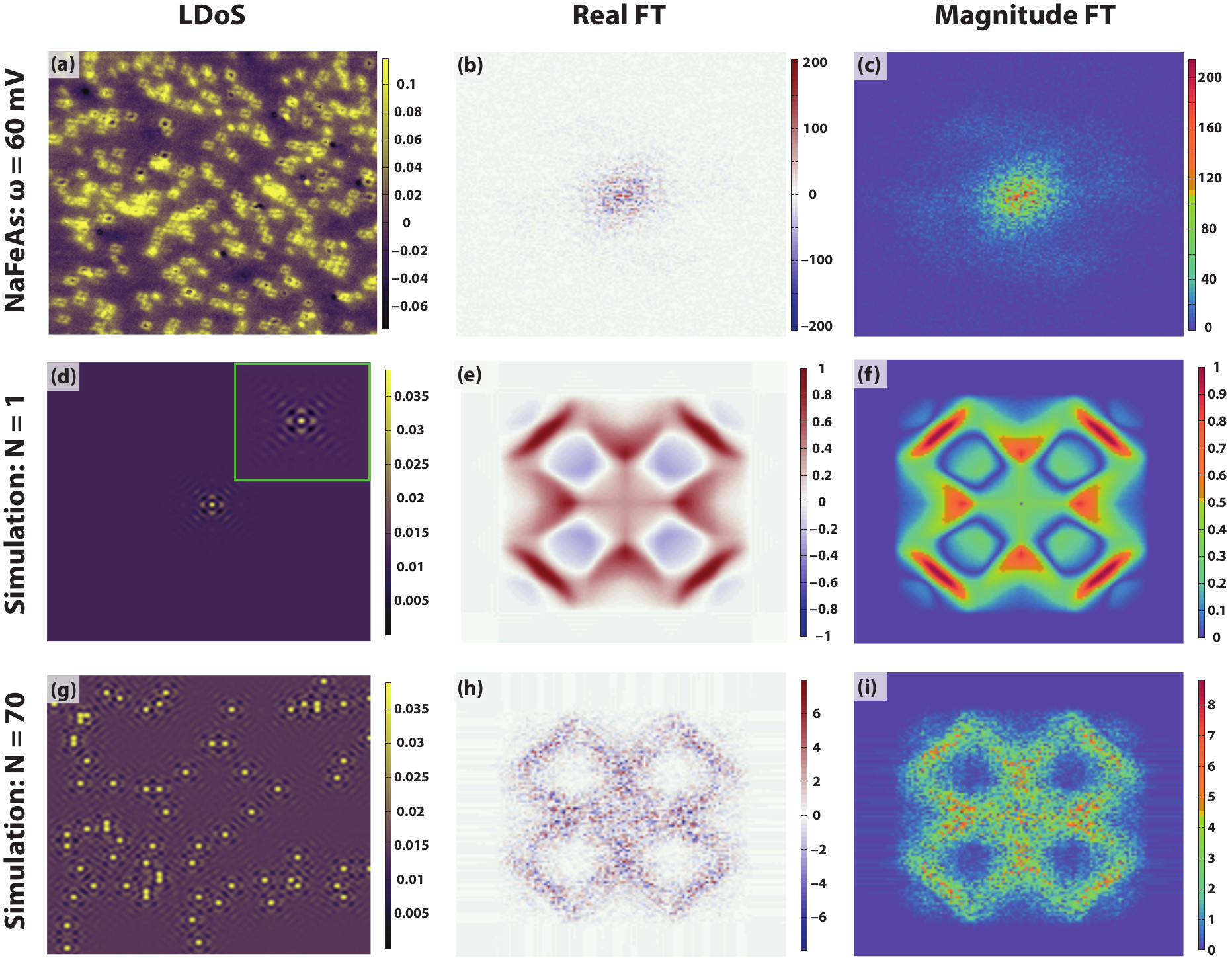
Figure 1: Shortcomings of the Fourier transform analysis. (a) The experimentally-obtained LDoS of NaFeAs over a $100\times 100$ nm² area of the sample at energy $\omega=60$ mV from Ref Rosenthal et al., 2014 with junction conditions $V=-100$ mV and $I=300$ pA measured at $T=26$ K. (b)-(c) Real part and magnitude, respectively, of the FT of (a) showing large phase noise. (d) Simulated image of scattering from a single point defect. (e)-(f) Real part and magnitude, respectively, of the FT of (d). The LDoS scale in (d) was chosen such that the FT magnitude for the simulated single defect had a maximum of 1. (g)-(i) Corresponding simulated LDoS and FTs for scattering from 70 point defects that are randomly distributed in space. All FT spectra are shown for $-3\pi/5a\leq k_{x},k_{y}\leq 3\pi/5a$. Comparison with the single defect case shows that noise in the FTs arises from the random placement of defects. Furthermore, the maximum amplitude of the FT scales approximately as $\sqrt{N}$, resulting in a loss of signal fidelity in the FT analysis.

According to scattering theory, the FT of the QPI image of an individual defect, $\delta\rho_{0}(\vec{k},\omega)=\int\mathop{}\!\mathrm{d}\vec{x}\,e^{-i\vec{k}\cdot\vec{x}}\delta\rho_{0}(\vec{x},\omega)$, is correlated with the underlying electronic structure of the material Wang and Lee (2003); Fiete and Heller (2003); Kivelson et al. (2003). Most materials of interest have sufficient disorder so that the LDoS signatures of different defects overlap. In this situation, it is not possible to identify the isolated defect signature through inspection. Instead, the traditional analysis Arguello et al. (2015) proceeds by taking the FT of the entire STM image $\delta\rho(\vec{x},\omega)$ in (1):

$$\delta\rho(\vec{k},\omega)=\int\mathop{}\!\mathrm{d}\vec{x}\,e^{-i\vec{k}\cdot\vec{x}}\delta\rho(\vec{x},\omega)=\delta\rho_{0}(\vec{k},\omega)\sum_{j=1}^{N}c_{j}\exp\{-i\vec{k}\cdot\vec{x}_{j}\}$$ (2)

While the quantity of interest for QPI analysis is $\delta\rho_{0}(\vec{k},\omega)$, the experimental FT image contains a frequency-varying, complex-valued phase factor, $\mathcal{P}(\vec{k})\equiv\sum_{j=1}^{N}c_{j}\exp\{-i\vec{k}\cdot\vec{x}_{j}\}$. This is illustrated in Figure 1(b), where the Real Part of the FT (Re-FT) displays wild oscillations due to $\mathcal{P}(\vec{k})$. To mitigate this, the Magnitude of the FT (mag-FT) is taken, and the analysis proceeds by assuming that $\mathcal{P}(\vec{k})$ is approximately constant in magnitude so that $\left|\mathcal{P}(\vec{k})\right|\approx\bar{c}\sqrt{N}$, where $\bar{c}$ is the average value of the $c_{j}$. The result of this procedure is illustrated in Figure 1(c), showing that debilitating noise still persists in the FT after taking the modulus. Moreover, the procedure of obtaining the mag-FT effectively eliminates half of the useful information in the complex-valued FT, annihilating all of the phase information from electron scattering processes originally present in real space. Intense peaks and contours in the real and imaginary parts of $\delta\rho(\vec{k},\omega)$ are experimental indicators of dominant scattering wavevectors and order parameter symmetries, which can reveal important properties about the superconducting gap function sign structure Hanaguri et al. (2009); Chi et al. (2014) and surface states of topological insulators Zhang et al. (2009); Okada et al. (2011). However, random phase noise fluctuations in experimental QPI spectra make comparisons with theoretical QPI calculations difficult Hirschfeld et al. (2015a).

An improved analysis technique to FT-STM would identify the location and the LDoS signature associated with each defect in a quantitatively-rigorous fashion that respects experimental and material-specific constraints. For instance, defects remain fixed in position across a series of STM images in which the measurement bias voltage is varied (see Figure 2). In this work, we present an analysis technique based on nonconvex optimization that possesses these desirable features while being broadly applicable to other forms of microscopy and image analysis.

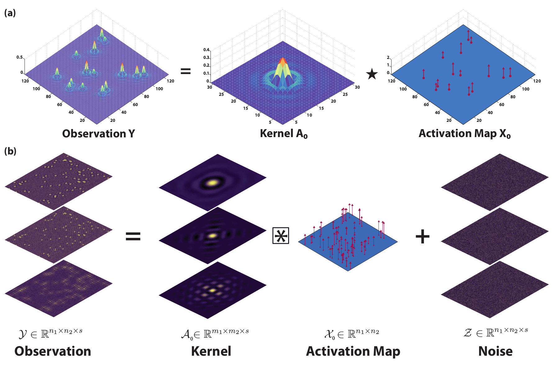
Figure 2: Convolutional data model for STM. (a) Schematic representation of the convolutional data model $\mathcal{Y}=\mathcal{A}_{0}\star\mathcal{X}_{0}$ for a noise-free simulated STM measurement. (b) Schematic representation of STM analysis as a high-dimensional deconvolution problem. Each constant-energy plane of $\mathcal{A}_{0}$ is convolved with the known activation map $\mathcal{X}_{0}$ and combined with additive noise $\mathcal{Z}$ to produce the noisy observation $\mathcal{Y}$. Algorithms for SBD seek to efficiently estimate $\mathcal{A}_{0}$ and $\mathcal{X}_{0}$ given the noisy measurement $\mathcal{Y}$.

Our algorithm is based on a deconvolutional procedure illustrated in Figure 2. The image (denoted as $\mathcal{Y}$) in Figure 2(a) was produced by simulating the effect of quasiparticle scattering from numerous point defects randomly distributed across the image. At a given bias voltage, the image consists of a recurrent scattering pattern (called the kernel $\mathcal{A}_{0}$) convolved with the locations and relative weights of each defect (called the activation map $\mathcal{X}_{0}$) as illustrated in Figure 2(a) and represented as $\mathcal{Y}=\mathcal{A}_{0}\star\mathcal{X}_{0}$. The underlying challenge in our analysis is to invert the procedure – starting with an STM image, determine the kernel and its corresponding activation map. The kernel and activation map are easily identified by inspection in Figure 2(a), however this becomes a highly non-trivial problem in the presence of many overlapping kernels and experimental noise. Similar convolutional models are used in neuroscience to model neuron spike patterns Pillow et al. (2013) and in systems biology to capture responses of the endocrine system Faghih et al. (2014). Hence an algorithm developed to solve this problem has broad applicability.

When $\mathcal{A}_{0}$ contains multiple slices, with each slice corresponding to a different bias voltage, we mathematically express the proposed model for STM measurements by collecting the convolutions for each voltage slice using the notation

$$\mathcal{Y}=\mathcal{A}_{0}\boxast\mathcal{X}_{0}+\mathcal{Z},$$ (3)

which is schematically depicted in Figure 2(b). The activation map $\mathcal{X}_{0}$ is shared globally across all measurement biases and $\mathcal{Z}$ is an additive noise tensor. The task of recovering both $\mathcal{A}_{0}$ and $\mathcal{X}_{0}$ given $\mathcal{Y}$ is known as the Sparse Blind Deconvolution (SBD) problem.

Over the last decade, a wealth of heuristics and applications for sparse signal recovery have been developed, often leading to efficient algorithms in theory as well as in practice Candes and Tao (2005); Elad (2012) (see Supplementary Information Section II). We investigate the following heuristic for producing estimates $\hat{\mathcal{A}}$ and $\hat{\mathcal{X}}$  for $\mathcal{A}_{0}$ and $\mathcal{X}_{0}$, by posing an optimization problem based on (3):

$$\hat{\mathcal{A}}=\operatorname*{arg\,min}_{\mathcal{A}}\min_{\mathcal{X}}\left[\psi_{\lambda}\left(\mathcal{A},\mathcal{X}\right)\equiv\frac{1}{2}\left\|\mathcal{A}\boxast\mathcal{X}-\mathcal{Y}\right\|_{F}^{2}+\lambda r(\mathcal{X})\right]$$ (4)

which allows one to recover $\mathcal{\hat{X}}=\operatorname*{arg\,min}_{\mathcal{X}}\psi_{\lambda}(\mathcal{\hat{A}},\mathcal{X})$.

This is similar to previous formulations proposed for various SBD applications: the Frobenius norm term $\left\|\cdot\right\|_{F}^{2}$ promotes data fidelity upon minimization $(\mathcal{Y}\simeq\mathcal{\hat{A}}\boxast\mathcal{\hat{X}})$, and a regularization term $r(\hat{\mathcal{X}})$ is chosen, such as the $\ell_{1}$ norm, so that the minimization encourages $\mathcal{\hat{X}}$ to be sparse, with $\lambda\geq 0$ governing the trade-off between the two objectives. However, most SBD applications focus on signal enhancement that uses the convolutional model as a rough guideline, leading to a weak notion of accurate estimation Levin et al. (2009). In contrast, the convolutional model fits naturally into the STM setting, in which robust, consistent results are paramount for scientific investigation. These considerations prompt a number of choices that are not emphasized in previous heuristics, such as the domain of $\mathcal{A}$, form of $r(\hat{\mathcal{X}})$, and refinement of the estimates.

In order to solve this optimization problem, we present the SBD-STM algorithm:

Algorithm 1 Complete SBD-STM Procedure

Input:

• Observation $\mathcal{Y}\in\mathbb{R}^{n_{1}\times n_{2}\times s}$, kernel size $\left(m_{1},m_{2}\right)$, initial $\lambda_{0}\geq 0$, decay rate $\alpha\in\left[0,1\right)$, and final $\lambda_{\mathrm{end}}\geq 0$.

Initial phase:

1. Randomly initialize: $\mathcal{A}^{\left(0\right)}\in\mathcal{S=\mathbb{S}}^{m_{1}\times m_{2}\times s}$.

2. $\mathcal{A}_{*}^{\left(0\right)},\mathcal{X}_{*}^{\left(0\right)}\leftarrow{\tt ASolve}\left(\mathcal{A}^{\left(0\right)},\lambda_{0},\mathcal{Y}\right)$.

Refinement phase:

1. Lifting: Get $\mathcal{A}^{\left(1\right)}\in S^{{}^{\prime}}=\mathcal{\mathbb{S}}^{m_{1}^{{}^{\prime}}\times m_{2}^{{}^{\prime}}\times s}$ by zero-padding the edges of $\mathcal{A}_{*}^{\left(0\right)}$ with a border of width $\left\lfloor\frac{m_{i}}{2}\right\rfloor$.

2. Set $\lambda_{1}=\lambda_{0}$.

3. Continuation: Repeat for $k=1,2,\dots$ until $\lambda_{k}\leq\lambda_{\mathrm{end}}$,

   1. $\mathcal{A}_{*}^{\left(k\right)},\mathcal{X}_{*}^{\left(k\right)}\leftarrow{\tt ASolve}\left(\mathcal{A}^{\left(k\right)},\lambda_{k},\mathcal{Y},\mathcal{X}_{*}^{\left(k-1\right)}\right)$,

   2. Centering:

      1. Find the size $m_{1}\times m_{2}$ submatrix of $\mathcal{A}_{*}^{\left(k\right)}$ that maximizes the Frobenius (square) norm across all $m_{1}\times m_{2}$ submatrices.

      2. Get $\mathcal{A}^{\left(k+1\right)}$ by shifting $\mathcal{A}_{*}^{\left(k\right)}$ so that the chosen $m_{1}\times m_{2}$ restriction is in the center, removing and zeropadding entries as needed.

      3. Normalize $\mathcal{A}^{\left(k+1\right)}$ so it lies in $\mathcal{S}^{{}^{\prime}}$.

      4. Shift $\mathcal{X}_{*}^{\left(k\right)}$ along the anti-parallel vector to the shift of $\mathcal{A}_{*}^{\left(k\right)}$.

   3. Set $\lambda_{k+1}=\alpha\lambda_{k}$.

Output:

1. Extract $\hat{\mathcal{A}}\in\mathcal{S}$ by extracting the restriction of the final $\mathcal{A}^{\left(k+1\right)}$ to the center $m_{1}\times m_{2}$ window.

2. Find the corresponding activation map $\hat{\mathcal{X}}\in\mathbb{R}^{n_{1}\times n_{2}}$ by solving $\min_{\mathcal{X}}\psi_{\lambda_{k}}\big{(}\hat{\mathcal{A}},\mathcal{X}\big{)}$.

 

Function Asolve

  Input:

• Current kernel, $\mathcal{A}_{in}$, current sparsity parameter, $\lambda_{in}$, the observation $\mathcal{Y}$, current activation map $\mathcal{X}_{in}$ (Refinement Phase)

Minimization

if Initial Phase then

    $\mathcal{X}_{1}\leftarrow$ Minimize $\mathcal{X}$ for $\psi_{\lambda_{in}}(\mathcal{A}_{in},\mathcal{X})$ using the FISTA algorithm Beck and Teboulle (2009).

else

    $\mathcal{X}_{1}\leftarrow\mathcal{X}_{in}$

end if

1. $\mathcal{A}_{out}\leftarrow$ Minimize $\mathcal{A}$ for $\psi_{\lambda_{in}}(\mathcal{A},\mathcal{X}_{1})$ using the Riemannian Trust-Region Method (RTRM) over the sphere Absil et al. (2007).

2. $\mathcal{X}_{out}\leftarrow$ Minimize $\mathcal{X}$ for $\psi_{\lambda_{in}}(\mathcal{A}_{out},\mathcal{X})$ using FISTA.

Output:

• $\mathcal{A}_{out}$, $\mathcal{X}_{out}$.

See Supplementary Information Sections II and III for further discussion on formulating and solving (4), and Section IV for how our approach to SBD can be applied to image deblurring by using an objective similar to (4).

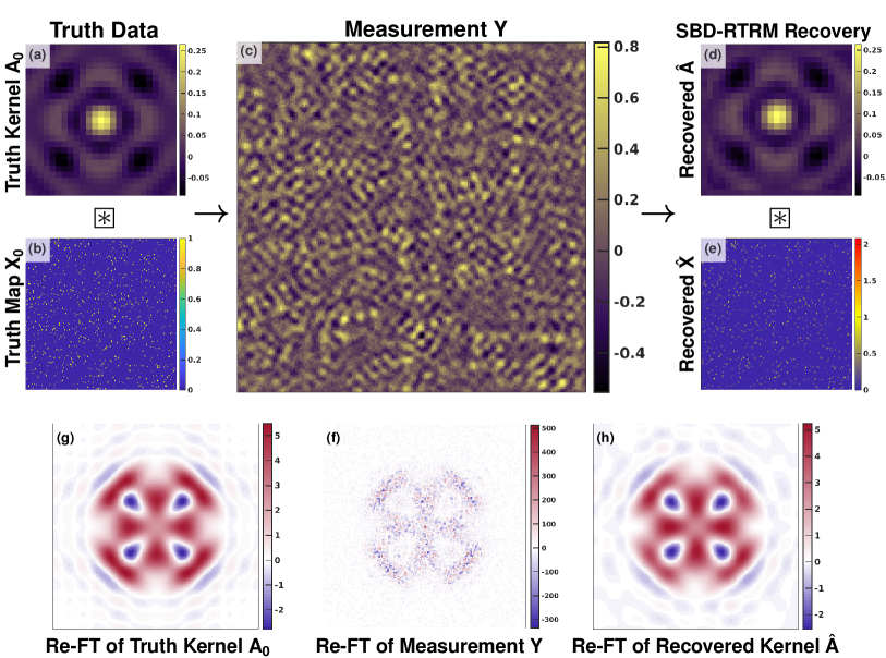
Figure 3: Illustrating the SBD-STM procedure. The simulated kernel (size $25\times 25$ pixels) in (a) is convolved with the activation map in (b) and added to random noise with $\textrm{SNR}\approx 0.792$ to produce the simulated noisy measurement shown in (c). The simulated measurement is a $185\times 185$ pixel image with a defect concentration of $\theta=2.73\%$. (d) Recovered kernel and (e) recovered activation map obtained using SBD-STM with $\lambda=0.1$, showing excellent agreement with simulation inputs in (a) and (b). The Re-FTs of the truth kernel, noisy measurement, and the recovered kernel from SBD-STM, shown in panels (f), (g), and (h), respectively. The Re-FT spectra are all shown with $-3\pi/5a\leq k_{x},k_{y}\leq 3\pi/5a$. The SBD-STM based FT shows both vastly improved SNR and a phase-sensitive recovery of the scattering interference.

To demonstrate the strength of SBD-STM, consider the situation illustrated in Figure 3. We generated a simulated observation $\mathcal{Y}$ using a ground truth scattering pattern $\mathcal{A}_{0}$ similar to Figure 1(d) and a dense, randomly generated activation map $\mathcal{X}_{0}$ shown in Figure 3(b). Convolving the truth data with the activation map and adding significant white noise with variance $\eta$ so that the Signal-to-Noise Ratio (SNR) is less than unity, with $\textrm{SNR}\equiv\frac{var(\mathcal{A}_{0})}{\eta}$, we generate the image shown in Figure 3(c). With many overlapping kernels and substantial noise, it is a futile task to accurately identify the underlying kernel and activation map of the image through visual inspection. However, as shown in Figure 3(d)-(e), SBD-STM successfully recovers a kernel $\hat{\mathcal{A}}$ and its associated activation map $\hat{\mathcal{X}}$ that closely resemble the truth data. The results shown in Figure 3 were obtained with a fixed $\lambda=0.1$. The scaling of the activation map entries is due to the choice of $\lambda$, and the noise also introduces blurring in the activation map Candès et al. (2008). Despite this, the overall features of the activation map and the recovered kernel are remarkably similar to the ground truth.

In Fourier space, the Re-FT of $\mathcal{Y}$ is missing crucial features of the true Re-FT spectrum and has noise fluctuations $\approx 100$ times that of the true transform. However, the Re-FT of the SBD-STM recovered kernel is consistent with the true Re-FT in both its structure and amplitude.

In our implementation, SBD-STM yields an activation map shared across all bias voltages. This not only reveals the spatial distribution of the defect kernels, but also naturally improves the accuracy of the SBD-STM recovered kernels at bias energies with noisy measurements. Consequently, SBD-STM returns more physically meaningful results when data from multiple biases are simultaneously analyzed than if each constant-bias slice of $\mathcal{Y}$ were individually analyzed. SBD-STM results on a simulated noisy STM dataset with 41 bias voltages are found in Supplementary Information Section V, demonstrating that SBD-STM is successful in optimizing the objective function with STM constraints in mind.

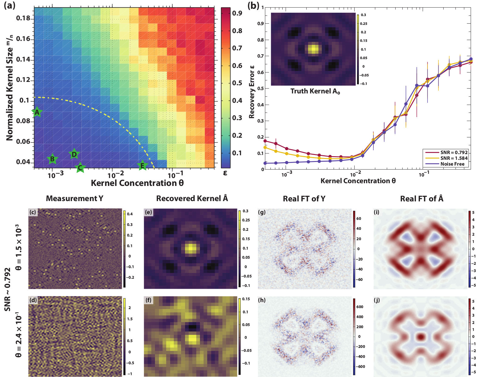
Figure 4: Benchmarking SBD-STM performance. (a) SBD-STM performance phase diagram from noise-free simulated results on images of area $n=256\times 256$, plotting the error metric $\epsilon(\hat{\mathcal{A}}_{\theta,\eta},\mathcal{A}_{0})$ as a function of normalized kernel size and concentration $\theta$ (the number of defects scaled by the number of pixels). Each point on the diagram is determined from the mean of 20 independent simulated measurements. SBD-STM performs well in the blue regions, but begins to fail in the red regions, at very high kernel size or concentration. The region where typical STM measurements are performed is bounded by the dashed line and the lower and left axes. Green stars labeled A, B, C, D, and E indicate representative images from Refs. Rutter et al., 2007; Roushan et al., 2009; Rosenthal et al., 2014; Arguello et al., 2015; Allan et al., 2013, respectively. (b) Performance of SBD-STM in the presence of additive noise in the measurement at a fixed value of the normalized kernel size $m/n=0.14$. (c)-(f) Examples of simulated measurements from panel (b) and their corresponding SBD-STM recovered kernels. (g)-(j) A comparison of the Re-FTs of the measurement and the SBD-STM recovered kernel, indicating that SBD-STM consistently outperforms FT-STM across all parameter ranges. All Re-FT spectra are shown with $-3\pi/5a\leq k_{x},k_{y}\leq 3\pi/5a$.

Before invoking SBD-STM on experimental data, we must understand its limitations and domain of applicability. The complexity of the STM deconvolution problem varies depending on the SNR and the overlap tendency of nearby defects. A series of numerical experiments on simulated data was performed to investigate the effects of defect concentration $\theta$ – the probability that any entry of $\mathcal{X}_{0}$ is “on” – and additive measurement noise on the expected success of SBD-STM. Simulated STM images are produced in a similar fashion as in Figure 3, and the performance of SBD-STM was assessed as a function of four adjustable parameters - the image size $n\equiv n_{1}\times n_{2}$, kernel size $m\equiv m_{1}\times m_{2}$, kernel concentration $\theta$, and SNR. Details of the data generation and simulation work are contained in Supplementary Information Sections I and VI. To assess the accuracy of kernel recovery in real space, we define the real space recovery error metric as $\epsilon(\hat{\mathcal{A}}_{\theta,\eta},\mathcal{A}_{0})\equiv\frac{2}{\pi}\arccos\left|\langle\hat{\mathcal{A}}_{\theta,\eta},\mathcal{A}_{0}\rangle\right|$, with $\langle\hat{\mathcal{A}}_{\theta,\eta},\mathcal{A}_{0}\rangle$ denoting the inner product of the vectorizations of $\hat{\mathcal{A}}_{\theta,\eta}$ and $\mathcal{A}_{0}$, which are the recovered and truth kernels, respectively. Figure 4(a) depicts a normalized defect size $\frac{m}{n}$ vs. concentration $\theta$ “phase diagram” to explore the interplay between $\frac{m}{n}$ and $\theta$ on real-space algorithmic accuracy $\epsilon(\hat{\mathcal{A}}_{\theta},\mathcal{A}_{0})$ in noise-free $(\eta=0)$ simulated measurements. We observe a phase transition in SBD-STM performance in the $\frac{m}{n}-\theta$ plane. The bottom-left of the plot captures situations in which the defects have negligible probability of overlapping, facilitating the near-perfect deconvolution of the noise free image. Increasing either $\frac{m}{n}$ or $\theta$ introduces error in the kernel recovery due to increased overlapping between defects. Practically, $\frac{m}{n}$ can be reduced by increasing the overall STM measurement area $n$ in an attempt to perform deconvolution-by-inspection. However at high defect concentrations $\theta$ or moderate noise levels, this strategy cannot guarantee success while SBD-STM can still return reliable estimates.

Next, we briefly discuss the SBD-STM performance as a function of noise in the signal. Figure 4(b) shows the evolution of $\epsilon(\hat{\mathcal{A}}_{\theta,\eta},\mathcal{A}_{0})$ as a function of defect concentration $\theta$ for three values of SNR ranging from noise free to noise-dominated (SNR $=0.792$). At high noise levels, performance error fluctuations in the far left of the plot appear because of the statistically futile challenge of accurately identifying low-density, low-intensity motifs under high levels of noise. The error curves appear to converge into a narrow band when $\theta\gtrsim 0.01$, demonstrating that the algorithm is robust to a wide range of SNRs for higher concentrations. By $\theta\approx 0.2$, the defect concentrations are sufficiently dense so that virtually all defect kernels are overlapping, causing SBD-STM to collapse and return unreliable estimates. These trends persist when the kernel size and SNR are further increased, as described in Supplementary Information Section VI. Altogether, our simulations show that in the range of parameters where typical STM experiments are performed (bounded by the dashed line in Figure 4(a)), SBD-STM performs splendidly ($\epsilon<0.1$) and consistently outperforms the usual FT-STM methodology even in the presence of considerable noise, as seen in Figure 4(c)-(j).

The results obtained above on synthetic data show that SBD-STM is able to recover kernels even at high defect density and in the presence of significant white noise, where alternate techniques such as manual detection fail. However, one might still question whether the method will work on real STM data, which might have other types of noise or errors which we have not accounted for in our synthetic data. In order to investigate this fully, we now apply SBD-STM to investigate a set of experimentally-obtained STM images of NaFe_1-xCo_xAs at different values of $x=0.0$, $0.015$ and $0.02$. At $x=0.0$ (parent compound), no additional cobalt dopants are present in the lattice, and the only defects present are those intrinsic to the crystal, which are at a concentration of about 1%. This compound has been previously studied via STM and the data have been analyzed using the standard Fourier transform technique  Rosenthal et al. (2014). To contrast with the standard FT-STM analysis, we implement SBD-STM on raw experimental data to demonstrate the significant improvement in data fidelity of the Re-FT. Shown in figure  5 (b) and (c) are the recovered Kernel and activation map respectively from the map shown in (a). Figure  5 (d) and (e) show the Re-FT of the entire image and of the kernel respectively over the same range in Fourier space. The phase sensitive recovery of the Fourier transform in Figure 5 (e) when compared to (d) is immediately apparent. We note that for this particular doping the individual kernels are well separated, and the kernel can be isolated directly by eye from the large area image in Figure 5(a). We show the application of SBD-STM to this sample to illustrate that the recovered kernel is indeed what one would expect by direct measurement around an individual defect.

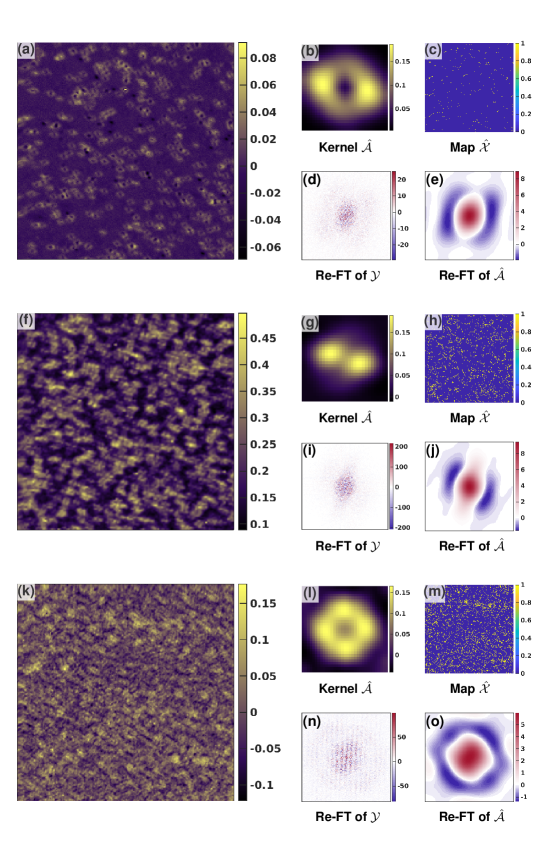
Figure 5: SBD-STM recoveries with increasing density of defects. In the left column, we have conductance maps with $\mathrm{Co}$ defects in NaFe_1-xCo_xAs of (a) high-quality ($T=71$ K, $I=59$ pA, $V_{set}=-100$ mV, $114\times 114$ nm), (f) $x=0.015$ ($T=6$ K, $I=-200$ pA, $V_{set}=-20$ mV, $50.4\times 50.4$ nm), and (k) $x=0.02$ ($T=5.9$ K, $I=200$ pA, $V_{set}=-50$ mV, $250\times 250$ nm) biased at energies of (a) $40$ meV, (f) $5$ meV, and (k) $-7$ meV. In the right column, clockwise from the top left, we have the recovered kernel (b,g,l), the recovered activation map (c,h,m), the Re-FT of the kernel (d,i,n), and the Re-FT of the conductance map (e,j,o), for comparison. The recovered kernels have been given 2-fold rotational symmetry, and all activations have been set to 1 to make them more readily visible.

We now turn to the sample with $x=0.015$, a STS image of which is shown in Figure 5(f). At this doping, we see that there are regions of high-density clustering of the kernels, where the clustering is dense enough such that the individual kernels overlap and become difficult to resolve. In Figure 5(g) and (h), we show the corresponding recovery for the kernel and activation map respectively. The Re-FT of the entire map and the recovered kernel are shown in Figure 5(i) and (j) respectively. At this defect level, we can very occasionally see isolated defects, and the recovered kernel is seen to nicely match with the differential conductance around these isolated defects.

Finally, we consider a sample that is optimally doped (highest $T_{c}$) with a nominal cobalt concentration of $x=0.02$. Shown in Figure 5(k) is an STS image obtained on this sample at $T=5.9$ K. At this doping level, there are no isolated impurities present anywhere in the sample, and the kernel can not be manually recovered. The SBD-STM is able to recover the kernel and activation map as shown in Figure 5(l) and (m) respectively. The Re-FT of the entire image and of the recovered kernel are shown in Figure 5(n) and (o) respectively. We see from the series of data in Figure 5 that SBD-STM works over the entire doping range that is relevant to STM experiments and is able to recover high-quality kernels with phase-sensitive Fourier transforms. As a side benefit of SBD-STM, we can obtain more accurate defect or dopant counts from the recovered activation maps.

From the results shown on both synthetic and real experimental STM data, we can see that SBD-STM provides a complete recovery of kernels in real space and therefore a phase sensitive recovery of the Fourier transform in reciprocal space. Within the formulation of quasiparticle interference, the phase of the Fourier transform in the QPI signal is dependent on the incoming and outgoing quasiparticle’s Green’s function as well as the potential of the impurity. The availability of phase information can give us new insight into individual materials that is not available simply from the magnitude of the QPI signal. In the remainder of this paper, we consider one such new insight into the physics of NaFe_1-xCo_xAs . NaFe_1-xCo_xAs , like many of the pnictides displays a superconducting dome as a function of cobalt doping. The maximum $T_{c}$ at optimal doping ($x=0.02$) reaches 18 K. As with the other pnictides, determining the symmetry of the superconducting order parameter in this compound is of much current interest. In this context, recent theoretical work on QPI in the superconducting state of the pnictides Hirschfeld et al. (2015b); Martiny et al. (2017) has opened up the possibility of distinguishing different superconducting order parameters from their QPI signature under the assumption that interband scattering in the superconducting state dominates the QPI signal. In Hirschfeld et al. (2015b), the (real) Fourier transform of the QPI signal around a single defect $\delta\rho(\vec{q},\omega)$ is integrated over momentum to produce the quantity $\delta\rho(\omega)$. This quantity is then anti-symmetrized with respect to energy relative to the Fermi level to produce a quantity $\delta\rho^{-}(\omega)=\delta\rho(\omega)-\delta\rho(-\omega)$. It is shown in Hirschfeld et al. (2015b) that in the case of $s^{\pm}$ pairing, $\delta\rho^{-}(\omega)$ is large and of constant sign over the energy range near the superconducting gap. Conversely, in the case of $s^{++}$ pairing, $\delta\rho^{-}(\omega)$ is expected to be small and have a sign change around the gap energy. In order to carry out the integration over $\vec{q}$ described in this procedure, it is required that we have access to the phase of the QPI signal. One way of achieving this is to directly image around an isolated dopant or defect where the complete phase sensitive pattern can be measured. Such STS imaging has recently been performed on iron chalcogenides Sprau et al. (2017); Du et al. (2017). However, this method has not been applied to the iron arsenides, especially at optimal doping where the defect or dopant density is high and the phase information in the FT was not previously available. Armed with the phase-sensitivity of SBD-STM, we now analyze differential conductance maps of near optimally doped NaFe_1-xCo_xAs to investigate the superconducting order parameter at optimal doping.

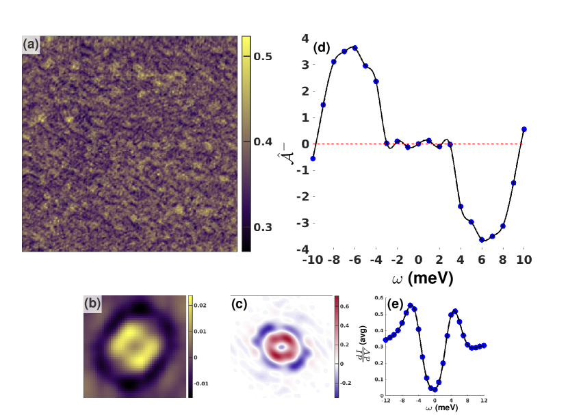
Figure 6: (a) Differential conductance map at $\omega=-10$ meV for an optimally doped NaFe_1-xCo_xAs sample (x=0.02), over a 250 nm $\times$ 250 nm field of view with $T=5.9$ K, $I=200pA$, and $V_{set}=-50$ meV. b) recovered kernel, $\mathcal{\hat{A}}$, from the conductance map in a). c) Fourier transform of the recovered kernel. d) $\mathcal{\hat{A}}^{-}(\omega)$, computed from the recovered kernels. The large and constant sign of the response is an indication of $s^{\pm}$ pairing. e) Spatially averaged differential conductance from the same area as a function of energy, revealing the superconducting gap 2$\Delta=11$ meV.

We start with a dataset that consists of 21 raw STS images from -10 meV to +10 meV in 1 meV increments on an optimally doped NaFe_1-xCo_xAs sample at T=5.9 K. One of these raw images at $\omega=-10$ meV is shown in Figure 6(a). Notice that no individual motifs can be resolved by eye. We then proceed to recover the kernels $\mathcal{\hat{A}}(\vec{r},\omega)$ at each energy using SBD-STM. An example of this recovery is shown in Figure 6(b), which is the recovered SBD-STM kernel $\mathcal{\hat{A}}(r,\omega=-10$ meV), recovered from the raw STS image in Figure 6(a). The recovered kernel lacks the strong anisotropy of recovered kernels from the underdoped regime, suggesting that electronic nematicity is not strong at this doping. Assuming that SBD-STM has worked correctly, the recovered $\mathcal{\hat{A}}(\vec{r},\omega)$ is identical to the real space QPI signal $\delta\rho(\vec{r},\omega)$. We then take the real-part of the 2-D Fourier transform $\mathcal{\hat{A}}(\vec{q},\omega)$, as shown in Figure 6(c) at $\omega=-10$ meV. This FT has the full phase information present, and we can then integrate over $\vec{q}$ and antisymmetrize with respect to energy:

$$\mathcal{\hat{A}^{-}}(\omega)=\sum_{\vec{q}}Re(\mathcal{\hat{A}}(\vec{q},\omega))-Re(\mathcal{\hat{A}}(\vec{q},-\omega))$$

We perform this procedure at each energy, and plot the resultant $\mathcal{\hat{A}}^{-}(\omega)$ in Figure 6(d). In (e), we show the spatially averaged differential conductance from the same data sets as a function of energy, revealing the superconducting gap. From the two coherence peaks, we calculate a $2\Delta$ of 11 meV. We can clearly see from Figure 6(d) that $\mathcal{\hat{A}}^{-}(\omega)$ is peaked near the superconducting gap, and has no sign change in the energy range near the gap, as expected for an $s^{\pm}$ order parameter. This procedure illustrates some of the new physical insight into STS image data that can be obtained once the complete phase information in the QPI signal is available for analysis.

In its current implementation, SBD-STM addresses the problem of identifying a single motif across a series of images. Beyond the identification of real space motifs in microscopy images, SBD-STM can also be applied to problems in which the motif is sparse in the appropriately chosen space, such as sparsity in the spatial gradient for natural image deblurring Fergus et al. (2006); Levin et al. (2011). Moreover, the flexibility of the convolutional data model in (3) affords the natural generalization, $\mathcal{Y}=\sum_{j=1}^{M}\mathcal{A}_{0}^{\left(j\right)}\boxast\mathcal{X}_{0}^{\left(j\right)}+\mathcal{Z}$, which expands the scope of SBD-STM to identify multiple distinct kernels in any series of images. In particular, STM images that contain various short-range orders, such as charge or spin density waves, would be amenable to a similar analysis Fujita et al. (2014); Arguello et al. (2015); Allan et al. (2013); Cai et al. (2013); Hamidian et al. (2016). SBD-STM recovered results from these STM measurements can be directly compared with theoretical predictions Knolle et al. (2010); Wang et al. (2015); Schattner et al. (2016) to understand the nature of competing orders in superconductors and other strongly correlated materials. Other analysis methodologies Fujita et al. (2014); Torre et al. (2016); Hamidian et al. (2016) have been recently proposed to improve FT data fidelity and provide some phase-sensitive information on the structure of ordered phases. These alternative approaches provide compelling information under suitable conditions, but their results are still vulnerable to phase noise contamination. The correct implementation of SBD-STM to such cases remains an open but solvable problem.

We thank Ethan Rosenthal and Erick Andrade for help with STM data acquisition, and Andrew Millis and Rafael Fernandes for discussions. This work is supported by the National Science Foundation Bigdata program (Grant number IIS-1546411). Support for STM equipment and operations is provided by the Air Force Office of Scientific Research (Grant number FA9550-16-1-0601).

References

- Crommie et al. (1993) M. F. Crommie, C. P. Lutz, and D. M. Eigler, “Imaging standing waves in a two-dimensional electron gas,” Nature 363, 524–527 (1993).
- Hoffman et al. (2002) J. E. Hoffman, K. McElroy, D.-H. Lee, K. M Lang, H. Eisaki, S. Uchida, and J. C. Davis, “Imaging quasiparticle interference in bi2sr2cacu2o8+x,” Science 297, 1148–1151 (2002).
- Rutter et al. (2007) G. M. Rutter, J. N. Crain, N. P. Guisinger, T. Li, P. N. First, and J. A. Stroscio, “Scattering and interference in epitaxial graphene,” Science 317, 219–222 (2007).
- Roushan et al. (2009) Pedram Roushan, Jungpil Seo, Colin V. Parker, Y. S. Hor, D. Hsieh, Dong Qian, Anthony Richardella, M. Z. Hasan, R. J. Cava, and Ali Yazdani, “Topological surface states protected from backscattering by chiral spin texture,” Nature 460, 1106–1109 (2009).
- Hanaguri et al. (2010) T. Hanaguri, S. Niitaka, K. Kuroki, and H. Takagi, “Unconventional s-wave superconductivity in fe(se,te),” Science 328, 474–476 (2010).
- Rosenthal et al. (2014) Ethan P. Rosenthal, Erick F. Andrade, Carlos J. Arguello, Rafael M. Fernandes, Ling Y. Xing, X. C. Wang, C. Q. Jin, Andrew J. Millis, and Abhay N. Pasupathy, “Visualization of electron nematicity and unidirectional antiferroic fluctuations at high temperatures in nafeas,” Nature Physics 10, 225–232 (2014).
- Arguello et al. (2015) C. J. Arguello, E. P. Rosenthal, E. F. Andrade, W. Jin, P. C. Yeh, N. Zaki, S. Jia, R. J. Cava, R. M. Fernandes, A. J. Millis, T. Valla, R. M. Osgood, and A. N. Pasupathy, “Quasiparticle interference, quasiparticle interactions, and the origin of the charge density wave in ,” Phys. Rev. Lett. 114, 037001 (2015).
- Wang and Lee (2003) Qiang-Hua Wang and Dung-Hai Lee, “Quasiparticle scattering interference in high-temperature superconductors,” Phys. Rev. B 67, 020511 (2003).
- Fiete and Heller (2003) Gregory A. Fiete and Eric J. Heller, “Colloquium : Theory of quantum corrals and quantum mirages,” Rev. Mod. Phys. 75, 933–948 (2003).
- Kivelson et al. (2003) S. A. Kivelson, I. P. Bindloss, E. Fradkin, V. Oganesyan, J. M. Tranquada, A. Kapitulnik, and C. Howald, “How to detect fluctuating stripes in the high-temperature superconductors,” Rev. Mod. Phys. 75, 1201–1241 (2003).
- McElroy et al. (2003) K. McElroy, R. W. Simmonds, J. E. Hoffman, D. H. Lee, J. Orenstein, H. Eisaki, S. Uchida, and J. C. Davis, “Relating atomic-scale electronic phenomena to wave-like quasiparticle states in superconducting bi2sr2cacu2o8+[delta],” Nature 422, 592–596 (2003).
- Pillow et al. (2013) Jonathan W. Pillow, Jonathon Shlens, E. J. Chichilnisky, and Eero P. Simoncelli, “A model-based spike sorting algorithm for removing correlation artifacts in multi-neuron recordings,” PLoS ONE 8, e62123 (2013).
- Faghih et al. (2014) Rose T. Faghih, Munther A. Dahleh, Gail K. Adler, Elizabeth B. Klerman, and Emery N. Brown, “Deconvolution of serum cortisol levels by using compressed sensing,” PLoS ONE 9, e85204 (2014).
- Betzig et al. (2006) Eric Betzig, George H. Patterson, Rachid Sougrat, O. Wolf Lindwasser, Scott Olenych, Juan S. Bonifacino, Michael W. Davidson, Jennifer Lippincott-Schwartz, and Harald F. Hess, “Imaging intracellular fluorescent proteins at nanometer resolution,” Science 313, 1642–1645 (2006).
- Muller (2009) David A. Muller, “Structure and bonding at the atomic scale by scanning transmission electron microscopy,” Nat Mater 8, 263–270 (2009).
- Binnig and Rohrer (1983) G. Binnig and H. Rohrer, “Surface imaging by scanning tunneling microscopy,” Ultramicroscopy 1, 157 – 160 (1983).
- Hanneken et al. (2015) C. Hanneken, F. Otte, A. Kubetzka, B. Dupe, N. Romming, K. von Bergmann, R. Wiesendanger, and S. Heinze, “Electrical detection of magnetic skyrmions by tunnelling non-collinear magnetoresistance,” Nature Nanotechnology 10, 1039–1042 (2015).
- Enayat et al. (2014) Mostafa Enayat, Zhixiang Sun, Udai Raj Singh, Ramakrishna Aluru, Stefan Schmaus, Alexander Yaresko, Yong Liu, Chengtian Lin, Vladimir Tsurkan, Alois Loidl, Joachim Deisenhofer, and Peter Wahl, “Real-space imaging of the atomic-scale magnetic structure of fe1+yte,” Science 345, 653–656 (2014).
- Kimoto et al. (2012) Koji Kimoto, Keiji Kurashima, Takuro Nagai, Megumi Ohwada, and Kazuo Ishizuka, “Assessment of lower-voltage {TEM} performance using 3d fourier transform of through-focus series,” Ultramicroscopy 121, 31 – 37 (2012).
- Jaffe and Glaeser (1987) J.S. Jaffe and R.M. Glaeser, “Difference fourier analysis of “surface features” of bacteriorhodopsin using glucose-embedded and frozen-hydrated purple membrane,” Ultramicroscopy 23, 17 – 28 (1987).
- Vonau et al. (2005) F. Vonau, D. Aubel, G. Gewinner, S. Zabrocki, J. C. Peruchetti, D. Bolmont, and L. Simon, “Evidence of hole-electron quasiparticle interference in semimetal by fourier-transform scanning tunneling spectroscopy,” Phys. Rev. Lett. 95, 176803 (2005).
- Simon et al. (2007) L. Simon, F. Vonau, and D. Aubel, “A phenomenological approach of joint density of states for the determination of band structure in the case of a semi-metal studied by ft-sts,” Journal of Physics: Condensed Matter 19, 355009 (2007).
- Wang and Lee (2011) Fa Wang and Dung-Hai Lee, “The electron-pairing mechanism of iron-based superconductors,” Science 332, 200–204 (2011).
- Hanaguri et al. (2009) T. Hanaguri, Y. Kohsaka, M. Ono, M. Maltseva, P. Coleman, I. Yamada, M. Azuma, M. Takano, K. Ohishi, and H. Takagi, “Coherence factors in a high-tc cuprate probed by quasi-particle scattering off vortices,” Science 323, 923–926 (2009).
- Chi et al. (2014) Shun Chi, S. Johnston, G. Levy, S. Grothe, R. Szedlak, B. Ludbrook, Ruixing Liang, P. Dosanjh, S. A. Burke, A. Damascelli, D. A. Bonn, W. N. Hardy, and Y. Pennec, “Sign inversion in the superconducting order parameter of lifeas inferred from bogoliubov quasiparticle interference,” Phys. Rev. B 89, 104522 (2014).
- Zhang et al. (2009) Tong Zhang, Peng Cheng, Xi Chen, Jin-Feng Jia, Xucun Ma, Ke He, Lili Wang, Haijun Zhang, Xi Dai, Zhong Fang, Xincheng Xie, and Qi-Kun Xue, “Experimental demonstration of topological surface states protected by time-reversal symmetry,” Phys. Rev. Lett. 103, 266803 (2009).
- Okada et al. (2011) Yoshinori Okada, Chetan Dhital, Wenwen Zhou, Erik D. Huemiller, Hsin Lin, S. Basak, A. Bansil, Y.-B. Huang, H. Ding, Z. Wang, Stephen D. Wilson, and V. Madhavan, “Direct observation of broken time-reversal symmetry on the surface of a magnetically doped topological insulator,” Phys. Rev. Lett. 106, 206805 (2011).
- Hirschfeld et al. (2015a) P. J. Hirschfeld, D. Altenfeld, I. Eremin, and I. I. Mazin, “Robust determination of the superconducting gap sign structure via quasiparticle interference,” Phys. Rev. B 92, 184513 (2015a).
- Candes and Tao (2005) E. J. Candes and T. Tao, “Decoding by linear programming,” IEEE Transactions on Information Theory 51, 4203–4215 (2005).
- Elad (2012) M. Elad, “Sparse and redundant representation modeling - what next?” IEEE Signal Processing Letters 19, 922–928 (2012).
- Levin et al. (2009) A. Levin, Y. Weiss, F. Durand, and W. T. Freeman, “Understanding and evaluating blind deconvolution algorithms,” in 2009 IEEE Conference on Computer Vision and Pattern Recognition (2009) pp. 1964–1971.
- Beck and Teboulle (2009) Amir Beck and Marc Teboulle, “A fast iterative shrinkage-thresholding algorithm for linear inverse problems,” SIAM Journal on Imaging Sciences 2, 183–202 (2009), https://doi.org/10.1137/080716542 .
- Absil et al. (2007) P.-A. Absil, C.G. Baker, and K.A. Gallivan, “Trust-region methods on riemannian manifolds,” Foundations of Computational Mathematics 7, 303–330 (2007).
- Candès et al. (2008) Emmanuel J. Candès, Michael B. Wakin, and Stephen P. Boyd, “Enhancing sparsity by reweighted ℓ 1 minimization,” Journal of Fourier Analysis and Applications 14, 877–905 (2008).
- Allan et al. (2013) M. P. Allan, T-M. Chuang, F. Massee, Yang Xie, Ni Ni, S. L. Bud’ko, G. S. Boebinger, Q. Wang, D. S. Dessau, P. C. Canfield, M. S. Golden, and J. C Davis, “Anisotropic impurity states, quasiparticle scattering and nematic transport in underdoped ca(fe1−xcoas2,” Nature Physics 9, 220–224 (2013).
- Hirschfeld et al. (2015b) P. J. Hirschfeld, D. Altenfeld, I. Eremin, and I. I. Mazin, “Robust determination of the superconducting gap sign structure via quasiparticle interference,” Phys. Rev. B 92, 184513 (2015b).
- Martiny et al. (2017) Johannes H. J. Martiny, Andreas Kreisel, P. J. Hirschfeld, and Brian M. Andersen, “Robustness of a quasiparticle interference test for sign-changing gaps in multiband superconductors,” Phys. Rev. B 95, 184507 (2017).
- Sprau et al. (2017) P. O. Sprau, A. Kostin, A. Kreisel, A. E. Böhmer, V. Taufour, P. C. Canfield, S. Mukherjee, P. J. Hirschfeld, B. M. Andersen, and J. C. Séamus Davis, “Discovery of orbital-selective cooper pairing in fese,” Science 357, 75–80 (2017), http://science.sciencemag.org/content/357/6346/75.full.pdf .
- Du et al. (2017) Zengyi Du, Xiong Yang, Dustin Altenfeld, Qiangqiang Gu, Huan Yang, Ilya Eremin, Peter?J Hirschfeld, Igor I. Mazin, Hai Lin, Xiyu Zhu, and Hai-Hu Wen, “Sign reversal of the order parameter in (li1-xfex)ohfe1-yznyse,” Nature Physics 14, 134 EP – (2017).
- Fergus et al. (2006) Rob Fergus, Barun Singh, Aaron Hertzmann, Sam T. Roweis, and William T. Freeman, “Removing camera shake from a single photograph,” ACM Trans. Graph. 25, 787–794 (2006).
- Levin et al. (2011) A. Levin, Y. Weiss, F. Durand, and W. Freeman, “Understanding blind deconvolution algorithms,” IEEE Transactions on Pattern Analysis and Machine Intelligence 33, 2354–2367 (2011).
- Fujita et al. (2014) Kazuhiro Fujita, Mohammad H. Hamidian, Stephen D. Edkins, Chung Koo Kim, Yuhki Kohsaka, Masaki Azuma, Mikio Takano, Hidenori Takagi, Hiroshi Eisaki, Shin-ichi Uchida, Andrea Allais, Michael J. Lawler, Eun-Ah Kim, Subir Sachdev, and J. C. Séamus Davis, “Direct phase-sensitive identification of a d-form factor density wave in underdoped cuprates,” Proceedings of the National Academy of Sciences 111, E3026–E3032 (2014).
- Cai et al. (2013) Peng Cai, Xiaodong Zhou, Wei Ruan, Aifeng Wang, Xianhui Chen, Dung-Hai Lee, and Yayu Wang, “Visualizing the microscopic coexistence of spin density wave and superconductivity in underdoped nafe1−xcoxas,” Nature Communications 4, 1596 (2013).
- Hamidian et al. (2016) M. H. Hamidian, S. D. Edkins, Chung Koo Kim, J. C. Davis, A. P. Mackenzie, H. Eisaki, S. Uchida, M. J. Lawler, E.-A. Kim, S. Sachdev, and K. Fujita, “Atomic-scale electronic structure of the cuprate d-symmetry form factor density wave state,” Nature Physics 12, 150–156 (2016).
- Knolle et al. (2010) J. Knolle, I. Eremin, A. Akbari, and R. Moessner, “Quasiparticle interference in the spin-density wave phase of iron-based superconductors,” Phys. Rev. Lett. 104, 257001 (2010).
- Wang et al. (2015) Yuxuan Wang, Daniel F. Agterberg, and Andrey Chubukov, “Coexistence of charge-density-wave and pair-density-wave orders in underdoped cuprates,” Phys. Rev. Lett. 114, 197001 (2015).
- Schattner et al. (2016) Yoni Schattner, Max H. Gerlach, Simon Trebst, and Erez Berg, “Competing orders in a nearly antiferromagnetic metal,” Phys. Rev. Lett. 117, 097002 (2016).
- Torre et al. (2016) Emanuele G. Dalla Torre, Yang He, and Eugene Demler, “Holographic maps of quasiparticle interference,” Nature Physics 12, 1052–1056 (2016).