EUROPEAN ORGANIZATION FOR NUCLEAR RESEARCH (CERN)

​​​ CERN-EP-2018-190 LHCb-PAPER-2018-024 3 June, 2019

Measurement of the relative ${{{B}^{-}}\!\rightarrow{{D}^{0}}/{{D}^{*0}}/{D^{**0}}{\mu^{-}}{{\overline{\nu}}_{\mu}}}$ branching fractions using ${B}^{-}$ mesons from ${\kern 3.73305pt\overline{\kern-3.73305ptB}{}}{}_{s2}^{*0}$ decays

LHCb collaboration

The decay of the narrow resonance ${{{\kern 1.79993pt\overline{\kern-1.79993ptB}{}}{}_{s2}^{*0}}\!\rightarrow{{B}^{-}}{{K}^{+}}}$ can be used to determine the ${B}^{-}$ momentum in partially reconstructed decays without any assumptions on the decay products of the ${B}^{-}$ meson. This technique is employed for the first time to distinguish contributions from ${D}^{0}$, ${D}^{*0}$, and higher-mass charmed states ($D^{**0}$) in semileptonic ${B}^{-}$ decays by using the missing-mass distribution. The measurement is performed using a data sample corresponding to an integrated luminosity of $3.0\mbox{\,fb}^{-1}$ collected with the LHCb detector in $pp$ collisions at center-of-mass energies of 7 and 8$\mathrm{\,Te\kern-1.00006ptV}$. The resulting branching fractions relative to the inclusive ${{{B}^{-}}\!\rightarrow{{D}^{0}}X{\mu^{-}}{{\overline{\nu}}_{\mu}}}$ are

$$f_{{{D}^{0}}}={\mathcal{B}}\quantity({{B}^{-}}\rightarrow{{D}^{0}}{\mu^{-}}{{\overline{\nu}}_{\mu}})/{\mathcal{B}}\quantity({{B}^{-}}\rightarrow{{D}^{0}}X{\mu^{-}}{{\overline{\nu}}_{\mu}}) =0.25\pm 0.06,$$

$$f_{{D^{**0}}}={\mathcal{B}}\quantity({{B}^{-}}\rightarrow\quantity({D^{**0}}\rightarrow{{D}^{0}}X){\mu^{-}}{{\overline{\nu}}_{\mu}})/{\mathcal{B}}\quantity({{B}^{-}}\rightarrow{{D}^{0}}X{\mu^{-}}{{\overline{\nu}}_{\mu}}) =0.21\pm 0.07,$$

with $f_{{D}^{*0}}=1-f_{{D}^{0}}-f_{D^{**0}}$ making up the remainder.

Published in Phys. Rev. D99 (2019) 092009

© 2024 CERN on behalf of the LHCb collaboration. CC-BY-4.0 licence.

 

1 Introduction

The composition of the inclusive bottom-to-charm semileptonic rate is not fully understood. Measurements of the exclusive branching fractions for ${{B}\!\rightarrow D\ell\nu}$ and ${{B}\!\rightarrow{{D}^{*}}\ell\nu}$ and corresponding decays with up to two additional charged pions [1] do not saturate the total ${b\!\rightarrow c}$ semileptonic rate as determined from analysis of the charged lepton’s kinematic moments [2, 3, 4]. One way to resolve this inclusive–exclusive gap is to make measurements of relative rates between different final states.

Semileptonic decays with excited charm states act as important backgrounds both to the exclusive decay channels ${B\!\rightarrow D\ell\nu}$ and ${B\!\rightarrow{{D}^{*}}\ell\nu}$ and for the study of semileptonic ${b\!\rightarrow u}$ transitions. For example, understanding these backgrounds is essential for experimental tests of lepton flavor universality studied by comparing the rates of tauonic and muonic $b$-hadron decays, e.g. $R(D^{(*)})\equiv{\mathcal{B}}\quantity({{\kern 1.79993pt\overline{\kern-1.79993ptB}{}}\!\rightarrow D^{(*)}{\tau^{-}}{{\overline{\nu}}_{\tau}}})/{\mathcal{B}}\quantity({{{\kern 1.79993pt\overline{\kern-1.79993ptB}{}}}\!\rightarrow D^{(*)}{\mu^{-}}{{\overline{\nu}}_{\mu}}})$ [5, 6, 7, 8, 9, 10, 11].

The largest contributions of excited charm states besides the $D^{*}(2007)^{0}$ or $D^{*}(2010)^{+}$ mesons come from the orbitally excited $L=1$ states $D_{0}^{*}\quantity(2400)$, $D_{1}\quantity(2420)$, $D_{1}\quantity(2430)$, and $D_{2}^{*}\quantity(2460)$, which have been individually measured [1]. We use the collective term $D^{**}$ to refer to these as well as other resonances such as radially excited $D$ mesons, and to nonresonant contributions with additional pions.

The contribution of excited states to the total semileptonic rate can be studied using $B$ decays in which the $B$ momentum is known. This allows one to calculate the mass of the undetected or “missing” part of the decay, and thus separate different excited $D$ states. In this paper we employ for the first time the technique described in Ref. [12] to accomplish this reconstruction in ${{{B}^{-}}\!\rightarrow{{D}^{0}}X{\mu^{-}}{{\overline{\nu}}_{\mu}}}$ decays, where $X$ refers to any number of additional particles, without assumptions about the decay products of the ${B}^{-}$ meson. There are three narrow peaks in the ${{B}^{-}}{{K}^{+}}$ mass distribution just above the mass threshold from decays of the orbitally excited $L=1$ ${\kern 1.79993pt\overline{\kern-1.79993ptB}{}}_{s}^{**}$ mesons [13, 14, 15]. We focus on the decay ${{{\kern 1.79993pt\overline{\kern-1.79993ptB}{}}{}_{s2}^{*0}}\!\rightarrow{{B}^{-}}{{K}^{+}}}$, which forms a narrow peak approximately $67\text{\,}\mathrm{Me\kern-1.00006ptV}$ above the threshold, and has the largest yield of any observed excited ${\kern 1.79993pt\overline{\kern-1.79993ptB}{}}{}^{0}_{s}$ state. By tagging ${B}^{-}$ mesons produced from the decay of these excited ${\kern 1.79993pt\overline{\kern-1.79993ptB}{}}{}_{s2}^{*0}$ mesons, the ${B}^{-}$ energy can be determined up to a quadratic ambiguity using the ${\kern 1.79993pt\overline{\kern-1.79993ptB}{}}{}_{s2}^{*0}$ and ${B}^{-}$ decay vertices and by imposing mass constraints for the ${B}^{-}$ and ${\kern 1.79993pt\overline{\kern-1.79993ptB}{}}{}_{s2}^{*0}$ mesons. Since only approximately 1% of ${B}^{-}$ mesons originate from a ${\kern 1.79993pt\overline{\kern-1.79993ptB}{}}{}_{s2}^{*0}$ decay, this method requires a large data set.

We determine the relative branching fractions of ${B}^{-}$ to ${D}^{0}$, ${D}^{*0}$, and $D^{**0}$, referred to as $f_{{D}^{0}}$, $f_{{D}^{*0}}$, and $f_{D^{**0}}$ respectively, in the ${{{B}^{-}}\!\rightarrow{{D}^{0}}X{\mu^{-}}{{\overline{\nu}}_{\mu}}}$ channel by fitting the distribution of the missing mass for ${{{\kern 1.79993pt\overline{\kern-1.79993ptB}{}}{}_{s2}^{*0}}\!\rightarrow{{B}^{-}}{{K}^{+}}}$ candidates. A similar set of fractions (along with their ${\kern 1.79993pt\overline{\kern-1.79993ptB}{}}{}^{0}$ counterparts), where the charge of the final state $D$ meson is not specified, has been measured previously at the BaBar experiment [16]. From the derivations in Ref. [17], we expect based on previous branching fraction measurements

$$f_{{{D}^{0}}} ={\mathcal{B}}\quantity({{B}^{-}}\rightarrow{{D}^{0}}{\mu^{-}}{{\overline{\nu}}_{\mu}})/{\mathcal{B}}\quantity({{B}^{-}}\rightarrow{{D}^{0}}X{\mu^{-}}{{\overline{\nu}}_{\mu}}) =0.235\pm 0.011^{+0.018}_{-0.012},$$

$$f_{{{D}^{*0}}} ={\mathcal{B}}\quantity({{B}^{-}}\rightarrow{{D}^{*0}}{\mu^{-}}{{\overline{\nu}}_{\mu}})/{\mathcal{B}}\quantity({{B}^{-}}\rightarrow{{D}^{0}}X{\mu^{-}}{{\overline{\nu}}_{\mu}}) =0.564\pm 0.017^{+0.042}_{-0.028},$$

$$f_{{D^{**0}}} ={\mathcal{B}}\quantity({{B}^{-}}\rightarrow\quantity({D^{**0}}\rightarrow{{D}^{0}}X){\mu^{-}}{{\overline{\nu}}_{\mu}})/{\mathcal{B}}\quantity({{B}^{-}}\rightarrow{{D}^{0}}X{\mu^{-}}{{\overline{\nu}}_{\mu}}) =0.201\pm 0.020^{+0.039}_{-0.060},$$

where the first uncertainty is experimental and the second gives an envelope of different extrapolation hypotheses to explain the inclusive–exclusive gap. Precise measurements of the relative branching fractions can distinguish between the hypotheses. Higher values in the $D^{**0}$ envelope (20% or more) would point towards a scenario in which there is a large contribution of unmeasured excited charm states. Lower fractions, closer to 14%, would suggest that the currently measured exclusive decays correctly describe the makeup of the total rate, and the inclusive–exclusive gap is due to other systematic effects.

A description of the data samples and selections used in this paper may be found in Sect. 2. Afterwards we discuss the missing mass reconstruction and related variables in Sect. 3. Along with the signal ${\kern 1.79993pt\overline{\kern-1.79993ptB}{}}{}_{s2}^{*0}$ decays, a large fraction of background decays are also selected. Yields and missing mass shapes must be determined for each of the background categories as described in Sect. 4. The most important background source is semileptonic decays of ${B}^{-}$ and ${\kern 1.79993pt\overline{\kern-1.79993ptB}{}}{}^{0}$ mesons with the same final state as the signal that do not originate from ${\kern 1.79993pt\overline{\kern-1.79993ptB}{}}{}_{s2}^{*0}$ decays. After accounting for other sources of background in Sect. 4.1, we estimate the yield and shape of this source in Sect. 4.2. The relative branching fractions are determined using a template fit to the missing mass distribution as described in Sect. 5. The systematic uncertainties included in the fit are then described in Sect. 6. The final result is presented in Sect. 7.

2 Data sample and selection

The LHCb detector [18, 19] is a single-arm forward spectrometer covering the pseudorapidity range $2<\eta<5$, designed for the study of particles containing $b$ or $c$ quarks. The detector includes a high-precision tracking system consisting of a silicon-strip vertex detector surrounding the $pp$ interaction region [20], a large-area silicon-strip detector located upstream of a dipole magnet with a bending power of about $4{\mathrm{\,Tm}}$, and three stations of silicon-strip detectors and straw drift tubes [21] placed downstream of the magnet. The tracking system provides a measurement of momentum, $p$, of charged particles with a relative uncertainty that varies from 0.5% at low momentum to 1.0% at 200$\mathrm{\,Ge\kern-1.00006ptV}$. The minimum distance of a track to a primary vertex (PV), the impact parameter (IP), is measured with a resolution of $(15+29/p_{\mathrm{T}}){\,\upmu\mathrm{m}}$, where $p_{\mathrm{T}}$ is the component of the momentum transverse to the beam, in $\mathrm{\,Ge\kern-1.00006ptV}$. Different types of charged hadrons are distinguished using information from two ring-imaging Cherenkov detectors [22]. Photons, electrons and hadrons are identified by a calorimeter system consisting of scintillating-pad and preshower detectors, an electromagnetic calorimeter and a hadronic calorimeter. Muons are identified by a system composed of alternating layers of iron and multiwire proportional chambers [23]. The online event selection is performed by a trigger [24], which consists of a hardware stage, based on information from the calorimeter and muon systems, followed by a software stage, which applies a full event reconstruction.

We use data samples collected in 2011 and 2012, at center-of-mass energies of $7\text{\,}\mathrm{Te\kern-1.00006ptV}$ and $8\text{\,}\mathrm{Te\kern-1.00006ptV}$ respectively, corresponding to an integrated luminosity of 3.0$\mbox{\,fb}^{-1}$. All ${B}^{-}$ candidates are selected from ${{D}^{0}}{\mu^{-}}$ combinations, with ${{{D}^{0}}\!\rightarrow{{K}^{-}}{{\pi}^{+}}}$. The final-state particles are formed from high-quality tracks required to be inconsistent with being produced at any primary collision vertex in the event. Loose particle-identification requirements are also applied to these tracks. The ${{K}^{-}}$ and ${{\pi}^{+}}$ candidates must form a high-quality vertex, and their combined mass must lie in the range $18401890\text{\,}\mathrm{Me\kern-1.00006ptV}$. The muon from the ${{D}^{0}}{\mu^{-}}$ candidate is required to pass the hardware trigger, which requires a transverse momentum of $p_{\mathrm{T}}>$1.48\text{\,}\mathrm{Ge\kern-1.00006ptV}$$ in the $7\text{\,}\mathrm{Te\kern-1.00006ptV}$ data or $p_{\mathrm{T}}>$1.76\text{\,}\mathrm{Ge\kern-1.00006ptV}$$ in the $8\text{\,}\mathrm{Te\kern-1.00006ptV}$ data. The software trigger requires a two-, three- or four-track secondary vertex with a significant displacement from any primary $pp$ interaction vertex, consistent with coming from a $b$ hadron. The ${{D}^{0}}{\mu^{-}}$ vertex must be of high quality, and well separated from the primary vertex.

After selecting ${B}^{-}$ candidates, we add candidate kaons consistent with originating from the primary vertex, referred to as prompt, to form the ${\kern 1.79993pt\overline{\kern-1.79993ptB}{}}{}_{s2}^{*0}$ candidates. To reduce background from misidentified pions from the primary interaction, we impose strong particle-identification requirements. The selection requirements for the prompt kaons are optimized using the fully reconstructed decay ${{{B}^{-}}\!\rightarrow{{J\mskip-3.0mu/\mskip-2.0mu\psi\mskip 2.0mu}}{{K}^{-}}}$. Signal decays produce a ${{B}^{-}}{{K}^{+}}$ pair; in addition to this opposite-sign kaon (OS$K$) data sample, we also use ${{B}^{-}}{{K}^{-}}$ same-sign kaon (SS$K$) combinations to help estimate backgrounds from data.

Samples of simulated ${\kern 1.79993pt\overline{\kern-1.79993ptB}{}}{}_{s2}^{*0}$ events are used to model the ${{{B}^{-}}\!\rightarrow{{D}^{0}}{\mu^{-}}{{\overline{\nu}}_{\mu}}}$, ${{{B}^{-}}\!\rightarrow{{D}^{*0}}{\mu^{-}}{{\overline{\nu}}_{\mu}}}$, and ${{{B}^{-}}\!\rightarrow{D^{**0}}{\mu^{-}}{{\overline{\nu}}_{\mu}}}$ signal components. For the $D^{**0}$ component, the simulation includes contributions from the four $L=1$ $D$ mesons as well as a small contributions of nonresonant $D^{(*)}\pi$ decays. In the simulation, $pp$ collisions are generated using Pythia [25, *Sjostrand:2007gs] with a specific LHCb configuration [27]. Decays of hadronic particles are described by EvtGen [28], in which final-state radiation is generated using Photos [29]. The interaction of the generated particles with the detector, and its response, are implemented using the Geant4 toolkit [30, *Agostinelli:2002hh] as described in Ref. [32].

3 Reconstruction of the $\boldsymbol{{{B}^{-}}}$ meson momentum

We find the energy of the ${B}^{-}$ meson by using its flight direction from the primary vertex to the secondary ${{D}^{0}}{\mu^{-}}$ vertex; a diagram of the decay topology is shown in Fig. 1. Applying mass constraints for the ${B}^{-}$ meson mass, $m_{B}$, and the hypothesized parent particle mass, $m_{BK}$, leaves a quadratic equation for the ${B}^{-}$ meson energy, $E_{B}$, derived in Appendix A.

Figure 1: Decay topology for the ${{{B}^{-}}\!\rightarrow{{D}^{0}}X{\mu^{-}}{{\overline{\nu}}_{\mu}}}$ signal decays. A ${\kern 1.61993pt\overline{\kern-1.61993ptB}{}}{}_{s2}^{*0}$ meson decays at the primary vertex position, producing a ${B}^{-}$ meson and a ${K}^{+}$ meson. The angle in the laboratory frame between the ${K}^{+}$ and ${B}^{-}$ directions is defined as $\theta$. The ${B}^{-}$ meson then decays semileptonically to a ${D}^{0}$ meson and a muon, accompanied by an undetected neutrino and potentially other particles, referred to collectively as $X$.

In carrying out the analysis we use two different quantities related to this calculation. The first is the minimum mass of the ${{B}^{-}}{{K}^{\pm}}$ pair. For a particular ${B}^{-}$ vertex and kaon track, there is a minimum $m_{BK}$ mass hypothesis for which the ${B}^{-}$ energy solutions are real. At this value, the discriminant of the quadratic equation is zero. This minimum mass value is given by

$$m_{\mathrm{min}}=\sqrt{m_{B}^{2}+m_{K}^{2}+2m_{B}\sqrt{p_{K}^{2}\sin^{2}\theta+m_{K}^{2}}},$$ (1)

where $p_{K}$ is the kaon momentum in the laboratory frame, $m_{K}$ is the kaon mass, and $\theta$ is the angle between the kaon direction and the direction from the primary to the secondary vertex. The distribution of the difference between $m_{\mathrm{min}}$ and the $m_{B}+m_{K}$ threshold, $\Delta m_{\mathrm{min}}=m_{\mathrm{min}}-m_{B}-m_{K}$, shown in Fig. 2 for both the OS$K$ and SS$K$ data samples, has excesses corresponding to the ${\kern 1.79993pt\overline{\kern-1.79993ptB}{}}{}_{s2}^{*0}$ and ${\kern 1.79993pt\overline{\kern-1.79993ptB}{}}{}_{s1}^{0}$ states even for decays that are not fully reconstructed. We use these distributions in a control region of $0<\Delta m_{\mathrm{min}}<$220\text{\,}\mathrm{Me\kern-1.00006ptV}$$ to constrain the total amount of ${\kern 1.79993pt\overline{\kern-1.79993ptB}{}}{}_{s2}^{*0}$ decays and non-${\kern 1.79993pt\overline{\kern-1.79993ptB}{}}{}_{s2}^{*0}$ background contributions in our selection, as described in more detail in Sect. 4.

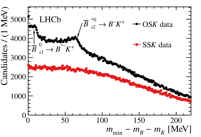
Figure 2: Distribution of the minimum mass difference for ${{B}^{-}}{{K}^{+}}$ (OS$K$) candidates and ${{B}^{-}}{{K}^{-}}$ (SS$K$) candidates. For OS$K$ combinations, peaks for the ${\kern 1.61993pt\overline{\kern-1.61993ptB}{}}{}_{s2}^{*0}$ and ${\kern 1.61993pt\overline{\kern-1.61993ptB}{}}{}_{s1}^{0}$ states are visible. The contribution of decays in which a kaon from a $b$-hadron decay is chosen as prompt produces the sharp increase near zero. The SS$K$ sample is used for background estimation.

Decays of ${\kern 1.79993pt\overline{\kern-1.79993ptB}{}}{}_{s1}^{0}$ mesons and background candidates where a secondary kaon is misidentified as coming from the primary interaction have small values of $\Delta m_{\mathrm{min}}$; the latter produces the increase near zero seen in Fig. 2. To remove these, we define our signal region for the missing mass fit as $30<\Delta m_{\mathrm{min}}<$67\text{\,}\mathrm{Me\kern-1.00006ptV}$$.

The second quantity is the missing mass, assuming the particles result from the decay of a ${\kern 1.79993pt\overline{\kern-1.79993ptB}{}}{}_{s2}^{*0}$ meson (imposing $m_{BK}=m_{{{\kern 1.25995pt\overline{\kern-1.25995ptB}{}}{}_{s2}^{*0}}}$). The energy of the ${B}^{-}$ meson, $E_{B}$, is calculated as follows:

$$E_{B} =\frac{\Delta^{2}}{2E_{K}}\frac{1}{1-\quantity(p_{K}/E_{K})^{2}\cos^{2}\theta}\quantity[1\pm\sqrt{d}],$$ (2)

where

$$\Delta^{2} =m_{{{\kern 1.25995pt\overline{\kern-1.25995ptB}{}}{}_{s2}^{*0}}}^{2}-m_{B}^{2}-m_{K}^{2},$$ (3)

and

$$d =\frac{p_{K}^{2}}{E_{K}^{2}}\cos^{2}\theta-\frac{4m_{B}^{2}p_{K}^{2}\cos^{2}\theta}{\Delta^{4}}\quantity(1-\frac{p_{K}^{2}}{E_{K}^{2}}\cos^{2}\theta).$$ (4)

Once $E_{B}$ has been determined, we calculate the missing mass squared

$$m_{\mathrm{miss}}^{2}=(p_{B}-p_{\mathrm{vis}})^{2},$$ (5)

where $p_{B}$ is the four momentum calculated from $E_{B}$ and the ${B}^{-}$ direction, and $p_{\mathrm{vis}}$ is the four momentum of the ${{D}^{0}}{\mu^{-}}$ combination. We require real solutions for Eq. 2. This keeps only candidates with $m_{\mathrm{min}}$ less than the ${\kern 1.79993pt\overline{\kern-1.79993ptB}{}}{}_{s2}^{*0}$ mass; candidates with $\Delta m_{\mathrm{min}}>m_{{{\kern 1.25995pt\overline{\kern-1.25995ptB}{}}{}_{s2}^{*0}}}-m_{B}-m_{K}$, which is approximately $67\text{\,}\mathrm{Me\kern-1.00006ptV}$, produce imaginary solutions. The $m_{\mathrm{miss}}^{2}$ variable is then used to perform the final fit to determine the relative branching fractions.

We keep only the physical solutions for $E_{B}$ which are greater than the sum of the energies of the reconstructed decay products. Based on simulation, approximately 75% of signal candidates have a physical solution. For candidates with two physical solutions, the one with lower energy is correct 90% of the time. Only the lower energy solution is used for these candidates. The difference $\Delta m_{\mathrm{miss}}^{2}$ between the reconstructed missing-mass squared and the corresponding true values for different classes of solutions are shown in Fig. 3. When $E_{B}$ is correctly reconstructed, the full-width at half maximum of the $\Delta m_{\mathrm{miss}}^{2}$ distribution is approximately $0.4\text{\,}{\mathrm{Ge\kern-1.00006ptV}}^{2}$ and is consistent among the signal channels. The resulting $m_{\mathrm{miss}}^{2}$ distributions for the signal decays to be used in the fit are shown in Fig. 4.

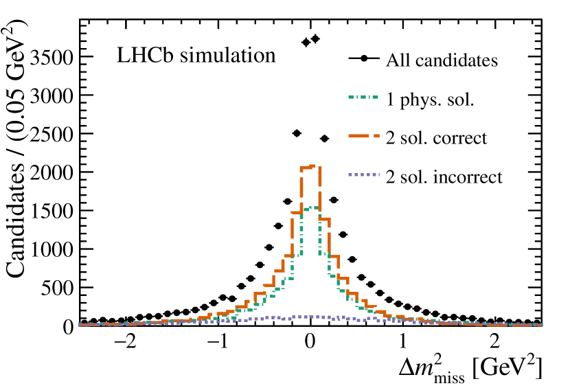
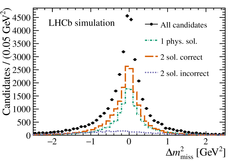
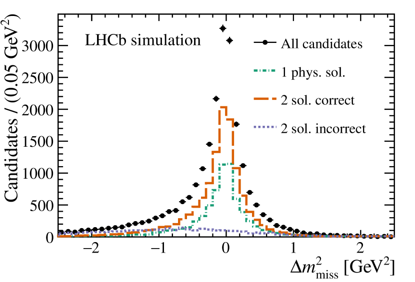
Figure 3: The difference $\Delta m_{\mathrm{miss}}^{2}$ between the reconstructed missing mass squared and the corresponding true values for the (top left) ${{{B}^{-}}\!\rightarrow{{D}^{0}}{\mu^{-}}{{\overline{\nu}}_{\mu}}}$ channel, (top right) the ${{{B}^{-}}\!\rightarrow{{D}^{*0}}{\mu^{-}}{{\overline{\nu}}_{\mu}}}$ channel, and (bottom) the ${{{B}^{-}}\!\rightarrow{D^{**0}}{\mu^{-}}{{\overline{\nu}}_{\mu}}}$ channel. The contributions from events in which there is only one physical solution, in which there are two and the chosen lower energy solution is correct, or in which the incorrect solution is chosen are shown.

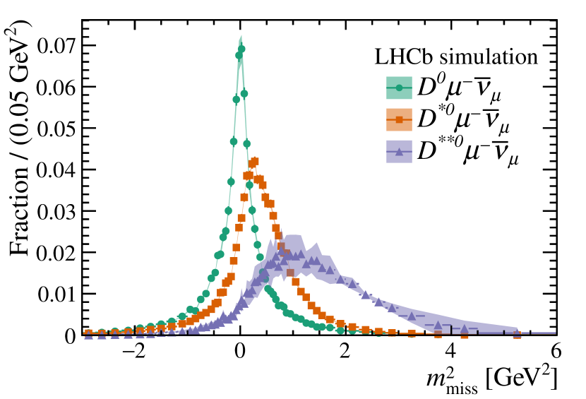
Figure 4: The missing mass shapes from simulation for the signal samples are shown. The bands around the points represent the systematic uncertainties on the form factors in the simulation and the branching fractions for different contributions to the $D^{**0}$ channel.

4 Background estimation

The backgrounds to the ${\kern 1.79993pt\overline{\kern-1.79993ptB}{}}{}_{s2}^{*0}$ signal candidates come from a number of different sources. For each of these sources, we estimate the overall yield as well as the missing-mass shapes. The most important sources are semileptonic decays of ${B}^{-}$ and ${\kern 1.79993pt\overline{\kern-1.79993ptB}{}}{}^{0}$ mesons not originating from a ${\kern 1.79993pt\overline{\kern-1.79993ptB}{}}{}_{s2}^{*0}$ or ${\kern 1.79993pt\overline{\kern-1.79993ptB}{}}{}_{s1}^{0}$ decay, which represent 83% of the total number of selected candidates.

The overall estimated background in the $m_{\mathrm{miss}}^{2}$ distribution is shown in Fig. 5. We make this estimation by first considering a number of smaller contributions not from semileptonic decays of ${B}^{-}$ and ${\kern 1.79993pt\overline{\kern-1.79993ptB}{}}{}^{0}$ mesons:

• misreconstructed backgrounds consisting of

  • non-${D}^{0}$ backgrounds,

  • ${{D}^{0}}{\mu^{-}}$ combinations not from the same $b$-hadron decay,

  • backgrounds with a hadron misidentified as the muon;

• ${\kern 1.79993pt\overline{\kern-1.79993ptB}{}}{}^{0}_{s}$ and ${\mathchar 28931\relax}^{0}_{b}$ semileptonic decays to final states including a ${D}^{0}$ meson.

Together, these backgrounds total 8% of all selected candidates. We estimate their yield and shape in both the $m_{\mathrm{miss}}^{2}$ and the $\Delta m_{\mathrm{min}}$ variables as described in Sect. 4.1. These can then be accounted for in both the distributions of the OS$K$ and SS$K$ data samples. We then estimate the semileptonic ${B}^{-}$ and ${\kern 1.79993pt\overline{\kern-1.79993ptB}{}}{}^{0}$ backgrounds as described in Sect. 4.2. The expectation for the ${\kern 1.79993pt\overline{\kern-1.79993ptB}{}}{}^{0}$ contribution is subtracted from the remaining SS$K$ sample, producing an estimate for the shape of the ${B}^{-}$ contribution in that sample. These two distributions are then extrapolated to the OS$K$ sample to produce the background estimation. The difference between this estimation and the full OS$K$ yield is composed of signal decays.

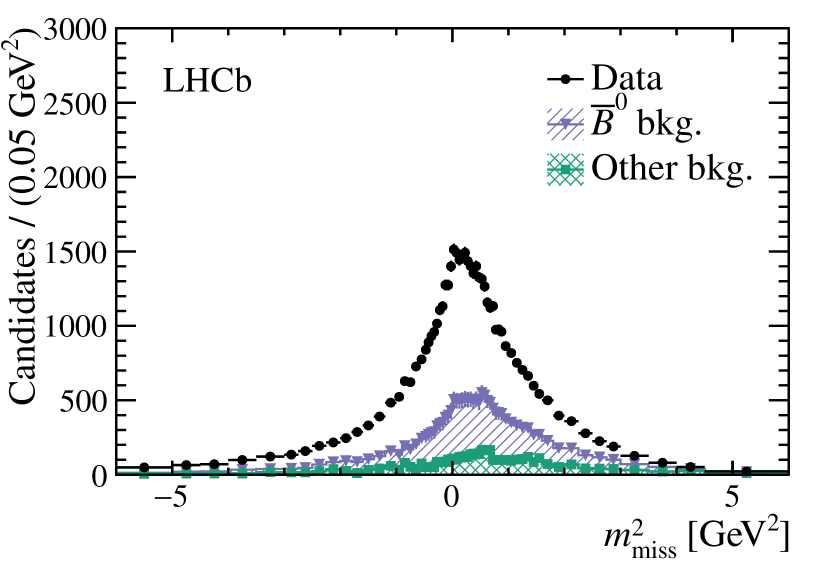
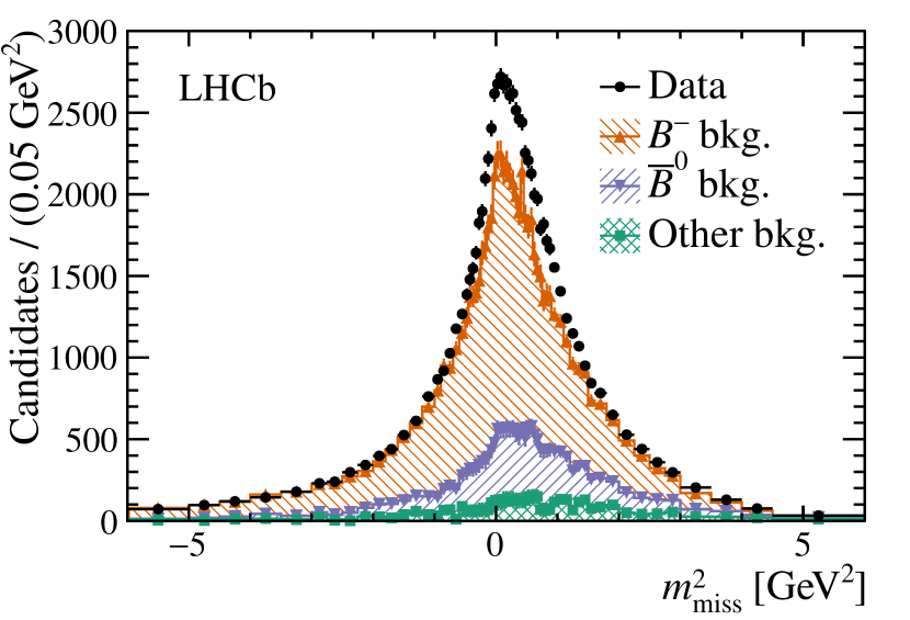
Figure 5: Missing-mass distribution for data and estimated background contributions in the (left) same-sign kaon sample and (right) opposite-sign sample. The other background decays include contributions from misreconstructed backgrounds, and semileptonic decays of ${\kern 1.61993pt\overline{\kern-1.61993ptB}{}}{}^{0}_{s}$ and ${\mathchar 28931\relax}^{0}_{b}$ mesons. The remainder of the SS$K$ sample not from ${\kern 1.61993pt\overline{\kern-1.61993ptB}{}}{}^{0}$ or other background decays is used to define the background contribution from ${B}^{-}$ semileptonic decays. This is then extrapolated to the OS$K$ sample, where the remainder is composed of signal. The background distributions are stacked.

4.1 Backgrounds not from semileptonic decays of $\boldsymbol{{{B}^{-}}}$ and $\boldsymbol{{{\kern 1.79993pt\overline{\kern-1.79993ptB}{}}{}^{0}}}$ mesons

Misreconstructed backgrounds are estimated using data-driven techniques. The yields and $\Delta m_{\mathrm{min}}$ and $m_{\mathrm{miss}}^{2}$ shapes of backgrounds without a ${D}^{0}$ meson are estimated using sidebands around the ${D}^{0}$ mass peak. The sideband ranges chosen are from $17901830\text{\,}\mathrm{Me\kern-1.00006ptV}$ and from $19001940\text{\,}\mathrm{Me\kern-1.00006ptV}$. The difference of the $m_{\mathrm{miss}}^{2}$ shape between the left and right sidebands is negligible. Approximately 3% of the selected candidates come from this background.

Combinations of ${{D}^{0}}{\mu^{-}}$ not coming from a single $b$-hadron decay are estimated using a wrong-sign (${{D}^{0}}{\mu^{+}}$) control sample, assuming that the doubly Cabbibo-suppressed contribution from ${{{D}^{0}}\!\rightarrow{{K}^{+}}{{\pi}^{-}}}$ is negligible. Along with this estimation, the contributions from misidentified muons to both the signal and wrong-sign samples are estimated using a control sample with particle-identification requirements that remove true muons. We then weight this sample using-particle identification efficiencies derived from calibration samples [33] to estimate the misidentified muon contamination. Together these two sources make up less than 1% of selected candidates.

We use a combination of data and simulation to estimate backgrounds from ${{{\kern 1.79993pt\overline{\kern-1.79993ptB}{}}{}^{0}_{s}}\!\rightarrow{{D}^{0}}K^{+}X{\mu^{-}}{{\overline{\nu}}_{\mu}}}$, ${{{\kern 1.79993pt\overline{\kern-1.79993ptB}{}}{}^{0}_{s}}\!\rightarrow{{D}^{0}}K^{0}X{\mu^{-}}{{\overline{\nu}}_{\mu}}}$, and ${{{\mathchar 28931\relax}^{0}_{b}}\!\rightarrow{{D}^{0}}pX{\mu^{-}}{{\overline{\nu}}_{\mu}}}$ decays. In data, additional candidates identified as kaons or protons, which are inconsistent with being produced at any primary collision vertex, are combined with the ${{D}^{0}}{\mu^{-}}$ candidates. This is done for both right- (${{D}^{0}}{{K}^{+}}$ or ${{D}^{0}}p$) and wrong-sign (${{D}^{0}}{{K}^{-}}$ or ${{D}^{0}}{\overline{p}}$) combinations. The wrong-sign combinations are used to model the combinatorial background in this selection. Using a-two dimensional fit to the ${{D}^{0}}K$ or ${{D}^{0}}p$ mass and the track impact parameter with respect to the ${{D}^{0}}{\mu^{-}}$ vertex, we determine the ${\kern 1.79993pt\overline{\kern-1.79993ptB}{}}{}^{0}_{s}$ and ${\mathchar 28931\relax}^{0}_{b}$ yields.

For the ${\kern 1.79993pt\overline{\kern-1.79993ptB}{}}{}^{0}_{s}$ case, the resulting yield is corrected for efficiency, and for modes with neutral kaons, using simulation. We take the shape of the contribution in $\Delta m_{\mathrm{min}}$ from simulation. There is an important contribution at low $\Delta m_{\mathrm{min}}$ where the kaon from the ${\kern 1.79993pt\overline{\kern-1.79993ptB}{}}{}^{0}_{s}$ decay points back to the primary vertex and is selected as the prompt kaon. This contribution is not present in the data control sample because of the requirement for the additional kaon to be inconsistent with any primary vertex. The final cut on $\Delta m_{\mathrm{min}}$ does, however, remove this component from the signal region. The simulated samples well reproduce the shape of the $\Delta m_{\mathrm{min}}$ distribution measured using the ${{D}^{0}}{{K}^{+}}X{\mu^{-}}$ selection.

Since the simulation does not reproduce well the shape in $m_{\mathrm{miss}}^{2}$ for the ${{D}^{0}}{{K}^{+}}X{\mu^{-}}$ control sample, the shape of the ${\kern 1.79993pt\overline{\kern-1.79993ptB}{}}{}^{0}_{s}$ contribution to the main $m_{\mathrm{miss}}^{2}$ fit is instead derived from the control sample. We obtain it by taking the difference in the right- and wrong-sign kaon $m_{\mathrm{miss}}^{2}$ distributions, scaling the wrong-sign yield to match the combinatorial contribution found by the two dimensional fit described above. The ${\kern 1.79993pt\overline{\kern-1.79993ptB}{}}{}^{0}_{s}$ contribution to the final selection is 3%, with a relative normalization uncertainty of 10%. For the ${\mathchar 28931\relax}^{0}_{b}$ case, the contribution is less than 1%. The shapes in both $\Delta m_{\mathrm{min}}$ and $m_{\mathrm{miss}}^{2}$ are taken from the control sample, and scaled based on the efficiency in simulation. The relative uncertainty on the normalization of this contribution is 20%. The $\Delta m_{\mathrm{min}}$ distribution for the sum of these backgrounds is shown in Fig. 6.

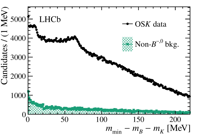
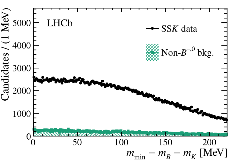
Figure 6: Distribution of the minimum mass difference for (left) ${{B}^{-}}{{K}^{+}}$ opposite-sign candidates and (right) ${{B}^{-}}{{K}^{-}}$ same-sign candidates. All candidates are compared to the estimated background from other sources besides decays of a ${B}^{-}$ or ${\kern 1.61993pt\overline{\kern-1.61993ptB}{}}{}^{0}$ meson to ${{D}^{0}}X{\mu^{-}}{{\overline{\nu}}_{\mu}}$. The remaining non-peaking part of the distributions is made up of ${B}^{-}$ and ${\kern 1.61993pt\overline{\kern-1.61993ptB}{}}{}^{0}$ semileptonic decays that do not come from an excited ${\kern 1.61993pt\overline{\kern-1.61993ptB}{}}{}^{0}_{s}$ state.

4.2 Backgrounds from semileptonic decays of $\boldsymbol{{{B}^{-}}}$ and $\boldsymbol{{{\kern 1.79993pt\overline{\kern-1.79993ptB}{}}{}^{0}}}$ mesons

We first estimate the number of candidates in the OS$K$ signal region that do not come from ${\kern 1.79993pt\overline{\kern-1.79993ptB}{}}{}_{s2}^{*0}$ decays. This is done with a fit to the $\Delta m_{\mathrm{min}}$ distribution in the control region after subtracting the backgrounds described in Sect. 4.1. The fit is done for three bins of prompt kaon $p_{\mathrm{T}}$ to account for the different spectra of the SS$K$ and OS$K$ samples: $0.5<p_{\mathrm{T}}<$1.25\text{\,}\mathrm{Ge\kern-1.00006ptV}$$, $1.25<p_{\mathrm{T}}<$2\text{\,}\mathrm{Ge\kern-1.00006ptV}$$, and $p_{\mathrm{T}}>$2\text{\,}\mathrm{Ge\kern-1.00006ptV}$$. The $\Delta m_{\mathrm{min}}$ shapes for ${{{\kern 1.79993pt\overline{\kern-1.79993ptB}{}}{}_{s2}^{*0}}\!\rightarrow{{B}^{-}}{{K}^{+}}}$ signals as well as ${\kern 1.79993pt\overline{\kern-1.79993ptB}{}}{}_{s1}^{0}$ and ${{{\kern 1.79993pt\overline{\kern-1.79993ptB}{}}{}_{s2}^{*0}}\!\rightarrow{B}^{*-}{{K}^{+}}}$, with ${{B}^{*-}\!\rightarrow{{B}^{-}}\gamma}$, backgrounds are taken from simulation. We model the background contribution using a fifth-order polynomial; the high order allows the fit to account for additional backgrounds peaking near $\Delta m_{\mathrm{min}}=0$.

In an alternative approach, the SS$K$ sample is scaled to model the background in the OS$K$ sample. The scaling is based on a linear fit to the ratio between OS$K$ and SS$K$ samples in the region $\Delta m_{\mathrm{min}}>$100\text{\,}\mathrm{Me\kern-1.00006ptV}$$, where the signal contribution is negligible. The $\Delta m_{\mathrm{min}}$ distributions, showing the results of these two methods of background estimation, are shown in Fig. 7. We use the difference of the two methods to estimate the systematic uncertainty on the background yield.

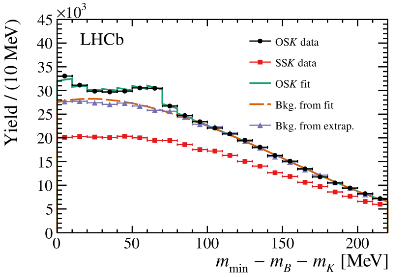
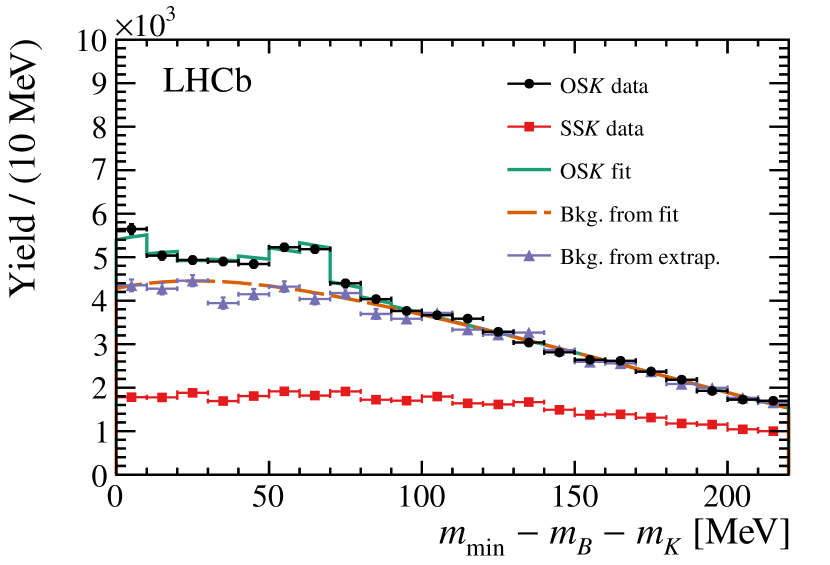
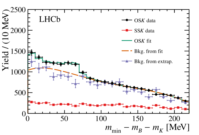
Figure 7: Fits to the opposite-sign and same-sign kaon $m_{\mathrm{min}}-m_{B}-m_{K}$ distributions with non-${B}^{-}$ and ${\kern 1.61993pt\overline{\kern-1.61993ptB}{}}{}^{0}$ backgrounds subtracted, and the resulting estimations of the non-${\kern 1.61993pt\overline{\kern-1.61993ptB}{}}{}_{s2}^{*0}$ and ${\kern 1.61993pt\overline{\kern-1.61993ptB}{}}{}_{s1}^{0}$ contributions. The fits are done separately in three bins of the prompt kaon $p_{\mathrm{T}}$: (top left) $0.5<p_{\mathrm{T}}<1.25\mathrm{\,Ge\kern-0.90005ptV}$, (top right) $1.25<p_{\mathrm{T}}<2\mathrm{\,Ge\kern-0.90005ptV}$, and (bottom) $p_{\mathrm{T}}>2\mathrm{\,Ge\kern-0.90005ptV}$. The dashed line shows the background estimation using a fit to the full OS$K$ distribution with signal templates from simulation and a fifth-order polynomial for the background. The points estimate the background using a linear extrapolation of the OS$K$ to SS$K$ ratio in the region $m_{\mathrm{min}}-m_{B}-m_{K}>100\mathrm{\,Me\kern-0.90005ptV}$.

The two methods constrain the yield of non-${\kern 1.79993pt\overline{\kern-1.79993ptB}{}}{}_{s2}^{*0}$ decays as a function of $\Delta m_{\mathrm{min}}$, however the missing-mass shape in the OS$K$ channel must still be determined. For each type of background decay, the missing-mass distribution is the same in the OS$K$ and SS$K$ samples for a particular value of $\Delta m_{\mathrm{min}}$. This equivalence is tested using fully reconstructed ${{{B}^{-}}\!\rightarrow{{J\mskip-3.0mu/\mskip-2.0mu\psi\mskip 2.0mu}}{{K}^{-}}}$ decays. However, since the missing mass also depends on the decay products, the distributions are different for ${B}^{-}$ and ${\kern 1.79993pt\overline{\kern-1.79993ptB}{}}{}^{0}$ decays. The fraction of this background coming from ${\kern 1.79993pt\overline{\kern-1.79993ptB}{}}{}^{0}$ decays is also different in the SS$K$ and OS$K$ samples.

We use the SS$K$ shape to model the background contribution in the OS$K$ sample, considering ${B}^{-}$ and ${\kern 1.79993pt\overline{\kern-1.79993ptB}{}}{}^{0}$ decays separately. This is done by estimating first the contribution of ${\kern 1.79993pt\overline{\kern-1.79993ptB}{}}{}^{0}$ decays to both the OS$K$ and SS$K$ channels. The remainder of the SS$K$ channel is used to model the shape of the ${B}^{-}$ contribution. The normalization of the ${B}^{-}$ background in the OS$K$ channel is then derived from the overall non-${\kern 1.79993pt\overline{\kern-1.79993ptB}{}}{}_{s2}^{*0}$ contribution with that from ${\kern 1.79993pt\overline{\kern-1.79993ptB}{}}{}^{0}$ mesons removed.

To estimate the fractional contribution from ${\kern 1.79993pt\overline{\kern-1.79993ptB}{}}{}^{0}$ decays in SS$K$ sample, we use the expected fraction resulting in the final state ${{D}^{0}}X{\mu^{-}}{{\overline{\nu}}_{\mu}}$ based on measured branching fractions [17]. The overlap with this measurement is removed by considering separately the ratio of contributions to the final state from ${\kern 1.79993pt\overline{\kern-1.79993ptB}{}}{}^{0}$ and ${B}^{-}$ decays for the ${{B}\!\rightarrow D^{*(*)}{\mu^{-}}{{\overline{\nu}}_{\mu}}}$ channels, $r_{D^{*(*)}}$, with ${D^{*(*)}\!\rightarrow{{D}^{0}}X}$. These ratios are combined with the measured fractions $f_{{{D}^{*0}}}$ and $f_{{D^{**0}}}$. We assume equal production of ${\kern 1.79993pt\overline{\kern-1.79993ptB}{}}{}^{0}$ and ${B}^{-}$ mesons. The fraction of ${\kern 1.79993pt\overline{\kern-1.79993ptB}{}}{}^{0}$ decays in the SS$K$ sample, $f_{{{\kern 1.25995pt\overline{\kern-1.25995ptB}{}}{}^{0}}}$, is thus given by

$$\frac{1}{f_{{{\kern 1.25995pt\overline{\kern-1.25995ptB}{}}{}^{0}}}} =\frac{{\mathcal{B}}\quantity({{{\kern 1.79993pt\overline{\kern-1.79993ptB}{}}{}^{0}}\!\rightarrow{{D}^{0}}X{\mu^{-}}{{\overline{\nu}}_{\mu}}})+{\mathcal{B}}\quantity({{{B}^{-}}\!\rightarrow{{D}^{0}}X{\mu^{-}}{{\overline{\nu}}_{\mu}}})}{{\mathcal{B}}\quantity({{{\kern 1.79993pt\overline{\kern-1.79993ptB}{}}{}^{0}}\!\rightarrow{{D}^{0}}X{\mu^{-}}{{\overline{\nu}}_{\mu}}})}$$

$$=1+\quantity[\frac{{\mathcal{B}}\quantity({{{\kern 1.79993pt\overline{\kern-1.79993ptB}{}}{}^{0}}\!\rightarrow{{D}^{*+}}{\mu^{-}}{{\overline{\nu}}_{\mu}}}){\mathcal{B}}\quantity({{{D}^{*+}}\!\rightarrow{{D}^{0}}X})+{\mathcal{B}}\quantity({{{\kern 1.79993pt\overline{\kern-1.79993ptB}{}}{}^{0}}\!\rightarrow D^{**+}{\mu^{-}}{{\overline{\nu}}_{\mu}}}){\mathcal{B}}\quantity({D^{**+}\!\rightarrow{{D}^{0}}X})}{{\mathcal{B}}\quantity({{{B}^{-}}\!\rightarrow{{D}^{0}}X{\mu^{-}}{{\overline{\nu}}_{\mu}}})}]^{-1}$$

$$=1+\quantity[r_{{{D}^{*}}}f_{D^{*0}}+r_{D^{**}}f_{D^{**0}}]^{-1}$$

$$=1+\quantity[(0.591\pm 0.024)f_{D^{*0}}+(1.00\pm 0.23)f_{D^{**0}}]^{-1}.$$ (6)

The uncertainty on $r_{{{D}^{*}}}$ comes chiefly from experimental uncertainty, while the dominant uncertainty on $r_{D^{**}}$ comes from extrapolation to the unmeasured parts of the semileptonic width. The uncertainty is taken as one standard deviation of the full extrapolation envelope assuming a uniform distribution. Using the central values of the expectations for $f_{{{D}^{*0}}}$ and $f_{{D^{**0}}}$ given in Sect. 1, the central value for $f_{{\kern 1.25995pt\overline{\kern-1.25995ptB}{}}{}^{0}}$ is 35%; variations within the uncertainties change it by approximately 2%. We then combine this value of $f_{{\kern 1.25995pt\overline{\kern-1.25995ptB}{}}{}^{0}}$ with an efficiency correction from simulation which depends on the lifetime difference between ${B}^{-}$ and ${\kern 1.79993pt\overline{\kern-1.79993ptB}{}}{}^{0}$ mesons.

The contribution from ${\kern 1.79993pt\overline{\kern-1.79993ptB}{}}{}^{0}$ mesons is studied similarly to the ${\kern 1.79993pt\overline{\kern-1.79993ptB}{}}{}^{0}_{s}$ and ${\mathchar 28931\relax}^{0}_{b}$ backgrounds, by attaching an additional candidate identified as a pion to the ${{D}^{0}}{\mu^{-}}$ candidates. We fit the ${{D}^{0}}\pi^{\pm}$ mass distributions, including peaking contributions from ${D}^{*+}$, $D_{1}$, and $D_{2}^{*}$ mesons on top of a smooth distribution. The normalizations of the peaks from the decay ${{{\kern 1.79993pt\overline{\kern-1.79993ptB}{}}{}^{0}}\!\rightarrow\quantity({D_{2}^{*+}\!\rightarrow{{D}^{0}}{{\pi}^{+}}}){\mu^{-}}{{\overline{\nu}}_{\mu}}}$ and the partially reconstructed decays ${{{\kern 1.79993pt\overline{\kern-1.79993ptB}{}}{}^{0}}\!\rightarrow\quantity({D_{1}^{+}\!\rightarrow{{D}^{*0}}{{\pi}^{+}}}){\mu^{-}}{{\overline{\nu}}_{\mu}}}$ and ${{{\kern 1.79993pt\overline{\kern-1.79993ptB}{}}{}^{0}}\!\rightarrow\quantity({D_{2}^{*+}\!\rightarrow{{D}^{*0}}{{\pi}^{+}}}){\mu^{-}}{{\overline{\nu}}_{\mu}}}$ show that there are more ${\kern 1.79993pt\overline{\kern-1.79993ptB}{}}{}^{0}$ candidates in the OS$K$ sample than there are in the SS$K$ sample. This is verified using fully reconstructed ${{{\kern 1.79993pt\overline{\kern-1.79993ptB}{}}{}^{0}}\!\rightarrow{{J\mskip-3.0mu/\mskip-2.0mu\psi\mskip 2.0mu}}{{\kern 1.99997pt\overline{\kern-1.99997ptK}{}}{}^{*}}\quantity(892)^{0}}$ decays. Combining the ratios in the two channels, we find there is a 10% larger contribution of ${\kern 1.79993pt\overline{\kern-1.79993ptB}{}}{}^{0}$ decays in the OS$K$ sample.

While the decays in the resonance peaks are dominated by either a ${B}^{-}$ or ${\kern 1.79993pt\overline{\kern-1.79993ptB}{}}{}^{0}$ initial state, the other contributions to the ${{D}^{0}}\pi^{\pm}$ distributions are more difficult to disentangle. The combinatorial background is expected to be symmetric in ${{D}^{0}}{{\pi}^{+}}{\mu^{-}}$ and ${{D}^{0}}{{\pi}^{-}}{\mu^{-}}$, while ${B}^{-}$ decays produce ${{D}^{0}}{{\pi}^{+}}{{\pi}^{-}}{\mu^{-}}$ which also contribute equally to both distributions. We therefore derive the ${\kern 1.79993pt\overline{\kern-1.79993ptB}{}}{}^{0}$ missing-mass shape by subtracting the ${{D}^{0}}{{\pi}^{-}}{\mu^{-}}$ shape from the ${{D}^{0}}{{\pi}^{+}}{\mu^{-}}$ shape. Each shape is corrected for the efficiency to reconstruct the additional pion based on simulation. The resulting distribution is validated using a simulated mixture of ${\kern 1.79993pt\overline{\kern-1.79993ptB}{}}{}^{0}$ decays.

We determine the total background shape from ${B}^{-}$ and ${\kern 1.79993pt\overline{\kern-1.79993ptB}{}}{}^{0}$ decays in the OS$K$ sample by first removing the expected ${\kern 1.79993pt\overline{\kern-1.79993ptB}{}}{}^{0}$ contribution from the initial SS$K$ sample’s $m_{\mathrm{miss}}^{2}$ distribution. This is then scaled up by 10% to estimate the ${\kern 1.79993pt\overline{\kern-1.79993ptB}{}}{}^{0}$ contribution to the OS$K$ sample. The remainder of the SS$K$ sample, composed of ${B}^{-}$ decays, is scaled up so that when it is added to the ${\kern 1.79993pt\overline{\kern-1.79993ptB}{}}{}^{0}$ estimate, the total number of background candidates in the OS$K$ sample is equal to the result of the $\Delta m_{\mathrm{min}}$ fit. We accomplish this procedure using an event-by-event weighting that accounts for the background yield as a function of $\Delta m_{\mathrm{min}}$.

Contributions not from semileptonic decays of ${B}^{-}$ and ${\kern 1.79993pt\overline{\kern-1.79993ptB}{}}{}^{0}$ mesons that are subtracted from the SS$K$ sample (${\kern 1.79993pt\overline{\kern-1.79993ptB}{}}{}^{0}_{s}$ and ${\mathchar 28931\relax}^{0}_{b}$ contributions, combinatorial, and misidentified muons) are also weighted in the same manner before being subtracted to produce the final background template.

4.3 Backgrounds from $\boldsymbol{{{\kern 1.79993pt\overline{\kern-1.79993ptB}{}}{}_{s2}^{*0}}}$ and $\boldsymbol{{{\kern 1.79993pt\overline{\kern-1.79993ptB}{}}{}_{s1}^{0}}}$ decays

The final class of backgrounds are ${\kern 1.79993pt\overline{\kern-1.79993ptB}{}}{}_{s}^{**0}$ decays that produce a ${B}^{-}$ meson with a ${{D}^{0}}{\mu^{-}}X$ final state that is not a semileptonic channel of interest. The $m_{\mathrm{miss}}^{2}$ shapes for semitauonic ${{{B}^{-}}\!\rightarrow{{D}^{0}}X\quantity({{\tau^{-}}\!\rightarrow{\mu^{-}}{{\overline{\nu}}_{\mu}}{{\nu}_{\tau}}}){{\overline{\nu}}_{\tau}}}$ decays and ${B}^{-}$ decays involving two charm mesons are estimated from simulation, and are included in the final fit. Contributions from ${\kern 1.79993pt\overline{\kern-1.79993ptB}{}}{}_{s1}^{0}$ or ${{{\kern 1.79993pt\overline{\kern-1.79993ptB}{}}{}_{s2}^{*0}}\!\rightarrow B^{*-}{{K}^{+}}}$, where ${B^{*-}\!\rightarrow{{B}^{-}}\gamma}$, are negligible after the requirement on the $\Delta m_{\mathrm{min}}$ variable.

5 Fit description

The fractions of interest, $f_{{D}^{0}}$ and $f_{D^{**0}}$, are determined from a binned-template, maximum-likelihood fit to the missing-mass distribution of the OS$K$ sample. The signal fraction $f_{{{D}^{*0}}}$ is given by the remainder, $1-f_{{{D}^{0}}}-f_{D^{**0}}$. To control statistical fluctuations in the templates for the missing-mass tails, which are important for determining the $D^{**0}$ content, a variable bin size is used for the template fit. The sum of the templates is allowed to vary bin-by-bin based on the combined statistical uncertainty of all templates. This variation is included using a single nuisance parameter for each bin that is constrained by the statistical uncertainty. It is dominated by the uncertainty of the SS$K$ sample used to create the combined ${B}^{-}$ and ${\kern 1.79993pt\overline{\kern-1.79993ptB}{}}{}^{0}$ background template. The effect of these uncertainty parameters is determined analytically using the Barlow–Beeston method [34]. Unless otherwise specified, we account for systematic uncertainties using nuisance parameters that are free to vary in the fit; these parameters are allowed to vary around their central values with a Gaussian constraint based on their uncertainty.

In total, the fit contains three signal and eight background templates: background from semileptonic ${B}^{-}$ and ${\kern 1.79993pt\overline{\kern-1.79993ptB}{}}{}^{0}$ decays not from a ${\kern 1.79993pt\overline{\kern-1.79993ptB}{}}{}_{s2}^{*0}$ decay, non-${D}^{0}$ backgrounds, ${{D}^{0}}{\mu^{-}}$ combinations not from the same $b$-hadron decay, backgrounds with a hadron misidentified as the muon, ${B}^{0}_{s}$, ${\mathchar 28931\relax}^{0}_{b}$, ${\kern 1.79993pt\overline{\kern-1.79993ptB}{}}{}_{s2}^{*0}$ decays with a semitauonic ${B}^{-}$ decay, and ${\kern 1.79993pt\overline{\kern-1.79993ptB}{}}{}_{s2}^{*0}$ decays with a ${B}^{-}$ decay to two charm mesons. There are 18 free parameters in the fit, not including the nuisance parameters for the template statistical uncertainties.

The three templates describing the signal are obtained from simulation—exclusive ${D}^{0}$, exclusive ${D}^{*0}$, and the sum of all $D^{**0}$ modes; these are shown in Fig. 4. We also correct for the relative reconstruction and selection efficiencies between these samples, which are taken from simulation. Relative to the ${D}^{*0}$ mode, the efficiency of the ${D}^{0}$ mode is 92% and that of the $D^{**0}$ mode is 68%. In addition to the two signal fractions of interest, three more free parameters govern the shape changes from the variations of the form factors, and one parameter gives the overall signal yield.

The template describing the ${B}^{-}$ and ${\kern 1.79993pt\overline{\kern-1.79993ptB}{}}{}^{0}$ backgrounds not coming from a ${\kern 1.79993pt\overline{\kern-1.79993ptB}{}}{}_{s2}^{*0}$ meson is extrapolated from the SS$K$ sample as described in Sect. 4. Four free parameters describe the systematic variations of the normalization as a function of $\Delta m_{\mathrm{min}}$. In the fit, the parameters $r_{{{D}^{*}}}$ and $r_{D^{**}}$ and the fractions $f_{{D}^{0}}$ and $f_{D^{**0}}$ are used to calculate $f_{{{\kern 1.25995pt\overline{\kern-1.25995ptB}{}}{}^{0}}}$ for the current evaluation of the fit function. This variation is constrained by the uncertainties of $r_{{{D}^{*}}}$ and $r_{D^{**}}$. The current value of $f_{{\kern 1.25995pt\overline{\kern-1.25995ptB}{}}{}^{0}}$ is combined with a set of templates that vary $f_{{{\kern 1.25995pt\overline{\kern-1.25995ptB}{}}{}^{0}}}$ by ${}\pm 1\%$ to extrapolate from the nominal value and produce the estimated background shape for this evaluation. An additional uncertainty in this template comes from the $m_{\mathrm{miss}}^{2}$ shape of the ${\kern 1.79993pt\overline{\kern-1.79993ptB}{}}{}^{0}$ component, which is controlled by one parameter.

The normalizations of the contributions from ${\kern 1.79993pt\overline{\kern-1.79993ptB}{}}{}^{0}_{s}$ decays, ${\mathchar 28931\relax}^{0}_{b}$ decays, and decays involving misidentified muons are also allowed to vary. The data-driven background shapes for fake and combinatorial muons, and for ${\kern 1.79993pt\overline{\kern-1.79993ptB}{}}{}^{0}_{s}$ and ${\mathchar 28931\relax}^{0}_{b}$ decays are described in Sect. 4.

The templates for the contribution of semitauonic decays of ${B}^{-}$ mesons from ${\kern 1.79993pt\overline{\kern-1.79993ptB}{}}{}_{s2}^{*0}$ are obtained from simulation. We determine the normalization relative to the semimuonic modes by deriving an effective ratio of semitauonic to semimuonic decays, $R\quantity({{D}^{0}}X)$, using the Standard Model values [35, 36, 37] and the expected fractions of ${D}^{0}$, ${D}^{*0}$, and $D^{**0}$,

$$R\quantity({{D}^{0}}X)=R\quantity(D)f_{{D}^{0}}+R\quantity(D^{*})f_{{D}^{*0}}+R\quantity(D^{**})f_{D^{**0}},$$ (7)

where $R\quantity(D)$ is the ratio ${\mathcal{B}}\quantity({{{\kern 1.79993pt\overline{\kern-1.79993ptB}{}}}\!\rightarrow D{\tau^{-}}{{\overline{\nu}}_{\tau}}})/{\mathcal{B}}\quantity({{{\kern 1.79993pt\overline{\kern-1.79993ptB}{}}}\!\rightarrow D{\mu^{-}}{{\overline{\nu}}_{\mu}}})$, and $R(D^{*})$ and $R(D^{**})$ are the corresponding ratios in the other decay channels. This is combined with the $\tau\rightarrow\mu X$ branching fraction [38] and the relative efficiency to reconstruct $\tau$ decays taken from simulation. The expected contribution is $\quantity(1.5\pm 0.3)\%$ of the selected ${\kern 1.79993pt\overline{\kern-1.79993ptB}{}}{}_{s2}^{*0}$ decays. The uncertainty is dominated by the difference of the Standard Model expectations and the world-average measured values of $R(D)$ and $R(D^{*})$ [1], which we take as a systematic uncertainty.

The other backgrounds coming from ${{{\kern 1.79993pt\overline{\kern-1.79993ptB}{}}{}_{s2}^{*0}}\!\rightarrow{{B}^{-}}{{K}^{+}}}$ decays are ${B}^{-}$ mesons decaying to double-charm states of various types. A simulated sample composed of many different decays producing ${{D}^{0}}{\mu^{-}}$ final states is used to determine the shape of this component. The normalization of the resulting missing-mass template is expected to be about 1% of ${\kern 1.79993pt\overline{\kern-1.79993ptB}{}}{}_{s2}^{*0}$ decays based on branching fractions, but is left unconstrained in the fit.

6 Systematic uncertainties

Each of the signal components has systematic uncertainties associated to its shape. The systematic uncertainty on the ${D}^{0}$ and ${D}^{*0}$ components is estimated based on uncertainties in the form-factor parameters. We reweight our simulated samples using the Caprini–Lellouch–Neubert (CLN) expansion formalism [39], with the uncertainties on the parameters taken from HFLAV [1]. This produces negligible changes in the missing mass template shapes compared to the other uncertainties in this analysis.

The uncertainty on the relative signal efficiencies is approximately 2%. We obtain the associated systematic uncertainty by repeating the fit with different efficiency values obtained by varying the efficiencies by their uncertainties.

For the $D^{**0}$ template, in addition to a large variation in the form-factor distribution based on results from Ref. [37], we create an alternative template with different branching fractions for the various resonant and nonresonant decay modes. The most important difference is the inclusion of a larger fraction of higher mass, nonresonant $D^{(*)}\pi$ and $D^{(*)}\pi\pi$ decays, where the pions may be of any allowed charge combination. This shape is fixed in the template fit; a second fit with the alternative template is used to estimate the systematic uncertainty from this shape. During this second fit, the signal efficiency of the $D^{**0}$ component is also adjusted along with the template. This uncertainty leads to the bands shown in Fig. 4.

For background contributions not from ${B}^{-}$ or ${\kern 1.79993pt\overline{\kern-1.79993ptB}{}}{}^{0}$ semileptonic decays, we include individual uncertainties on their normalizations. Systematic variations in the shapes are dominated by the statistical bin-by-bin statistical uncertainty.

We consider a number of systematic uncertainties on the ${B}^{-}$ and ${\kern 1.79993pt\overline{\kern-1.79993ptB}{}}{}^{0}$ contributions. The uncertainty due to the overall normalization comes from two sources. The statistical uncertainties in the polynomial background function of the $\Delta m_{\mathrm{min}}$ fit are used to modify the template. This corresponds to an uncertainty of less than 1% on the yield in each prompt kaon $p_{\mathrm{T}}$ bin. We also use the alternative extrapolation using the $\Delta m_{\mathrm{min}}$ ratio to provide an alternative normalization, giving an uncertainty of approximately 2%. Both of these uncertainties produce only small changes in the templates. The uncertainties in $r_{{{D}^{*}}}$ and $r_{D^{**}}$ give the uncertainty on the ${\kern 1.79993pt\overline{\kern-1.79993ptB}{}}{}^{0}$ fraction. The uncertainty in the ${\kern 1.79993pt\overline{\kern-1.79993ptB}{}}{}^{0}$ $m_{\mathrm{miss}}^{2}$ shape is estimated from the uncertainty in the efficiency from simulation to reconstruct the pion in the ${{D}^{0}}\pi^{\pm}{\mu^{-}}$ combination.

An estimated breakdown of the total statistical and systematic uncertainty is given in Table 1. The largest source of uncertainty is the statistical uncertainty from the extrapolated SS$K$ data sample. The uncertainty in the ${\kern 1.79993pt\overline{\kern-1.79993ptB}{}}{}^{0}$ $m_{\mathrm{miss}}^{2}$ shape is also important because of its effect on the high $m_{\mathrm{miss}}^{2}$ tail. Most systematic uncertainties are included in the fit with constrained nuisance parameters. The only source for which the fit result has a significantly smaller uncertainty than the initial constraint is the normalization of the non-${\kern 1.79993pt\overline{\kern-1.79993ptB}{}}{}_{s2}^{*0}$ background from the $\Delta m_{\mathrm{min}}$ extrapolation. For the final result, the total uncertainty is taken from the best fit, with the fixed systematic uncertainties for the relative signal efficiencies and the $D^{**0}$ branching fractions from added in quadrature.

Table 1: Estimates of the breakdown of the total uncertainty. All estimates are done by repeating the fit with systematic nuisance parameters fixed to their best fit values. The statistical uncertainty of the OS$K$ sample is estimated from the uncertainty on the signal fractions with the template statistical nuisance parameters fixed to their best fit values. The template statistical uncertainty is added in by allowing only the statistical nuisance parameters to vary. The effect of each floating systematic uncertainty is estimated by refitting with its systematic nuisance parameter shifted by the uncertainty found by the best fit and taking the difference in the signal fractions as the uncertainty. The total uncertainty is taken from the best fit, with the fixed systematic uncertainties added in quadrature.

Source of uncertainty		$f_{{D}^{0}}$	$f_{D^{**0}}$
Statistical	OS$K$ sample	$0.025$	$0.027$
	Templates	$0.047$	$0.052$
Floating syst.	Signal form-factors	$0.006$	$0.004$
	Non-${B}^{-}$, ${\kern 1.79993pt\overline{\kern-1.79993ptB}{}}{}^{0}$ backgrounds	$0.004$	$0.004$
	${B}^{-}$, ${\kern 1.79993pt\overline{\kern-1.79993ptB}{}}{}^{0}$ background normalization	$0.003$	$0.015$
	${\kern 1.79993pt\overline{\kern-1.79993ptB}{}}{}^{0}$ fraction and $m_{\mathrm{miss}}^{2}$ shape	$0.004$	$0.030$
Fixed syst.	$D^{**0}$ branching fractions	$0.025$	$0.044$
	Relative signal efficiency	$0.003$	$0.003$
Total uncertainty		0.056	$+0.070$
			$-0.074$

7 Results and conclusions

The result of the template fit is shown in Fig. 8. We find the parameters of interest

$$f_{{{D}^{0}}} =0.25\pm 0.06,$$

$$f_{{D^{**0}}} =0.21\pm 0.07,$$

where the uncertainty is the total due to statistical and systematic uncertainties. Contours for the 68.3% and 95.5% confidence intervals for the nominal fit are shown in Fig. 9. From the conditional covariance of the two parameters of interest combined with the fit result using alternate $D^{**0}$ branching fractions, the correlation coefficient of the two parameters is $\rho=-0.38$, which is dominated by the change in the alternate branching-fraction fit. The fraction $f_{{{D}^{*0}}}$ is equal to $1-f_{{{D}^{0}}}-f_{{D^{**0}}}=0.54\pm 0.07$, but this cannot be taken as an independent determination.

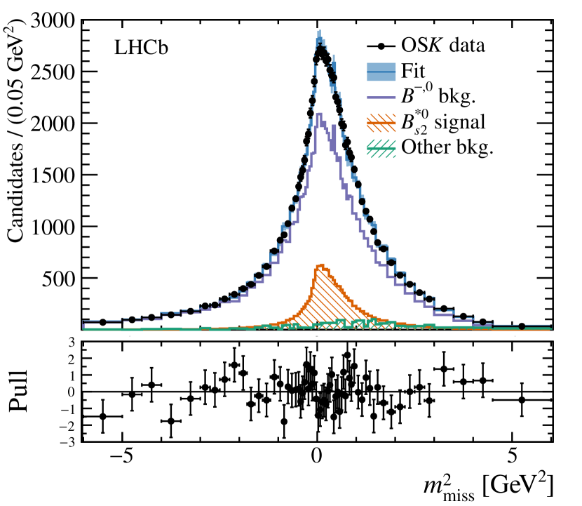
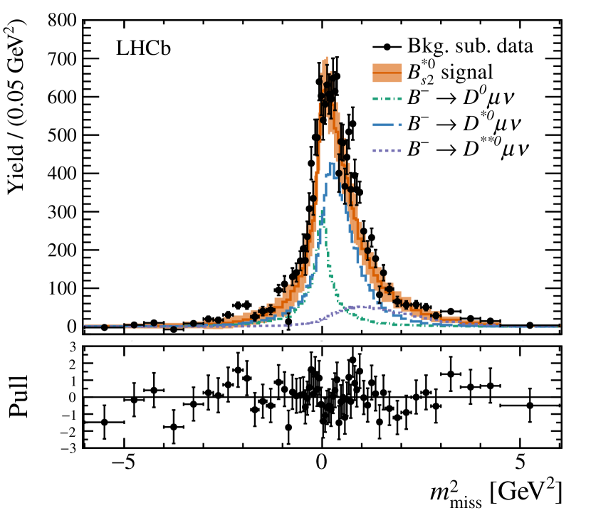
Figure 8: Template fit to the missing-mass distribution. The nuisance parameters used to quantify the template statistical uncertainties are set to their nominal values. The full distribution (left) is shown, comparing the background to the sum of the signal templates. The background-subtracted distribution (right) is compared to the breakdown of the signal components. The statistical uncertainty in the background templates is represented as the shaded band around the fit. In the pull distribution, the statistical uncertainty of the background templates is added to the statistical uncertainty of the data points.

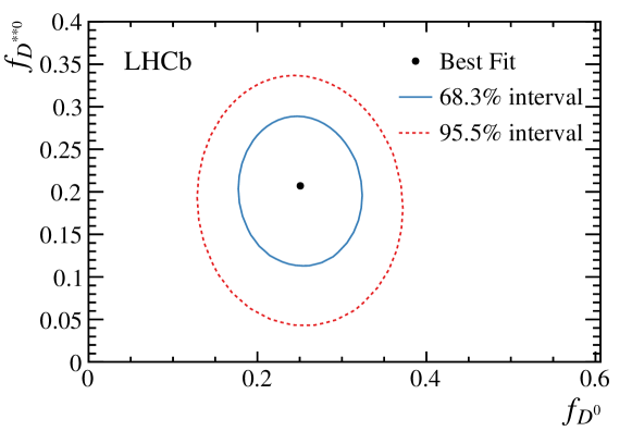
Figure 9: Contours for 68.3% and 95.5% confidence intervals for the fractions of ${{{B}^{-}}\!\rightarrow{{D}^{0}}X{\mu^{-}}{{\overline{\nu}}_{\mu}}}$ into the exclusive ${{{B}^{-}}\!\rightarrow{{D}^{0}}{\mu^{-}}{{\overline{\nu}}_{\mu}}}$ channel and the higher excited ${{{B}^{-}}\!\rightarrow\left({{D^{**0}}\!\rightarrow{{D}^{0}}X}\right){\mu^{-}}{{\overline{\nu}}_{\mu}}}$ channels. The alternate fit using different branching fractions for different $D^{**0}$ states is not included.

The results are compatible with expectations based on previous exclusive measurements [17]. Because of the uncertainty on the $D^{**0}$ component, the results do not yet favor a particular explanation for the exclusive–inclusive gap.

We have demonstrated that the reconstruction of the momentum of ${B}^{-}$ decays with missing particles using ${\kern 1.79993pt\overline{\kern-1.79993ptB}{}}{}_{s2}^{*0}$ decays is a viable method at the LHCb experiment. This technique requires much larger data sets than measurements with inclusive ${B}^{-}$ selections, but measuring the missing mass provides important discriminating power between different decay modes, and between signal and backgrounds. This is a promising method to employ with the additional data that the LHCb experiment has collected in Run 2 and will collect in the future.

Appendix

Appendix A Derivation of the $\boldsymbol{{{B}^{-}}}$ meson energy

Consider a known ${B}^{-}$ momentum direction with unknown energy and a kaon of momentum $p_{K}$ at an angle $\theta$ in the laboratory frame with respect to it. Taking the ${B}^{-}$ direction as the $z$-axis, the squared mass of the ${{B}^{-}}{{K}^{+}}$ system is

$$m_{BK}^{2} =\quantity|\matrixquantity(E_{B}\\ 0\\ 0\\ \sqrt{E_{B}^{2}-m_{B}^{2}})+\matrixquantity(\sqrt{p_{K}^{2}+m_{K}^{2}}\\ p_{K}\sin\theta\\ 0\\ p_{K}\cos\theta)|^{2}.$$ (8)

For a particular $$m_{BK}$$ hypothesis, Eq. 8 can be written

$$m_{BK}^{2} =\quantity(E_{B}+\sqrt{p_{K}^{2}+m_{K}^{2}})^{2}-p_{K}^{2}\sin^{2}\theta$$ (9)

$$\phantom{{}={}}-\quantity(\sqrt{E_{B}^{2}-m_{B}^{2}}+p_{K}\cos\theta)^{2}$$

$$=E_{B}^{2}+2E_{B}E_{K}+m_{K}^{2}+\quantity(p_{K}^{2}-p_{K}^{2}\sin^{2}\theta)$$ (10)

$$\phantom{{}={}}-E_{B}^{2}+m_{B}^{2}-2p_{K}\cos\theta\sqrt{E_{B}^{2}-m_{B}^{2}}-p_{K}^{2}\cos^{2}\theta.$$

Rearranging terms, squaring to remove the root, and using $$\Delta^{2}=m_{BK}^{2}-m_{B}^{2}-m_{K}^{2}$$ gives

$$0 =E_{B}^{2}\quantity(4\quantity(E_{K}^{2}-p_{K}^{2}\cos^{2}\theta))+E_{B}\quantity(-4E_{K}\Delta^{2})$$ (11)

$$\phantom{{}={}}+\quantity(4m_{B}^{2}p_{K}^{2}\cos^{2}\theta+\Delta^{4}).$$

The solution to the quadratic equation for $$E_{B}$$ is

$$E_{B} =\frac{\Delta^{2}}{2E_{K}}\frac{1}{1-\quantity(p_{K}/E_{K})^{2}\cos^{2}\theta}\quantity[1\pm\sqrt{d}],$$ (12)

where

$$d =\frac{p_{K}^{2}}{E_{K}^{2}}\cos^{2}\theta-\frac{4m_{B}^{2}p_{K}^{2}\cos^{2}\theta}{\Delta^{4}}\quantity(1-\frac{p_{K}^{2}}{E_{K}^{2}}\cos^{2}\theta).$$ (13)

LHCb collaboration

R. Aaij²⁷, B. Adeva⁴¹, M. Adinolfi⁴⁸, C.A. Aidala⁷³, Z. Ajaltouni⁵, S. Akar⁵⁹, P. Albicocco¹⁸, J. Albrecht¹⁰, F. Alessio⁴², M. Alexander⁵³, A. Alfonso Albero⁴⁰, S. Ali²⁷, G. Alkhazov³³, P. Alvarez Cartelle⁵⁵, A.A. Alves Jr⁴¹, S. Amato², S. Amerio²³, Y. Amhis⁷, L. An³, L. Anderlini¹⁷, G. Andreassi⁴³, M. Andreotti^16,g, J.E. Andrews⁶⁰, R.B. Appleby⁵⁶, F. Archilli²⁷, P. d’Argent¹², J. Arnau Romeu⁶, A. Artamonov³⁹, M. Artuso⁶¹, K. Arzymatov³⁷, E. Aslanides⁶, M. Atzeni⁴⁴, B. Audurier²², S. Bachmann¹², J.J. Back⁵⁰, S. Baker⁵⁵, V. Balagura^7,b, W. Baldini¹⁶, A. Baranov³⁷, R.J. Barlow⁵⁶, S. Barsuk⁷, W. Barter⁵⁶, F. Baryshnikov⁷⁰, V. Batozskaya³¹, B. Batsukh⁶¹, V. Battista⁴³, A. Bay⁴³, J. Beddow⁵³, F. Bedeschi²⁴, I. Bediaga¹, A. Beiter⁶¹, L.J. Bel²⁷, S. Belin²², N. Beliy⁶³, V. Bellee⁴³, N. Belloli^20,i, K. Belous³⁹, I. Belyaev^34,42, E. Ben-Haim⁸, G. Bencivenni¹⁸, S. Benson²⁷, S. Beranek⁹, A. Berezhnoy³⁵, R. Bernet⁴⁴, D. Berninghoff¹², E. Bertholet⁸, A. Bertolin²³, C. Betancourt⁴⁴, F. Betti^15,42, M.O. Bettler⁴⁹, M. van Beuzekom²⁷, Ia. Bezshyiko⁴⁴, S. Bhasin⁴⁸, J. Bhom²⁹, S. Bifani⁴⁷, P. Billoir⁸, A. Birnkraut¹⁰, A. Bizzeti^17,u, M. Bjørn⁵⁷, M.P. Blago⁴², T. Blake⁵⁰, F. Blanc⁴³, S. Blusk⁶¹, D. Bobulska⁵³, V. Bocci²⁶, O. Boente Garcia⁴¹, T. Boettcher⁵⁸, A. Bondar^38,w, N. Bondar³³, S. Borghi^56,42, M. Borisyak³⁷, M. Borsato⁴¹, F. Bossu⁷, M. Boubdir⁹, T.J.V. Bowcock⁵⁴, C. Bozzi^16,42, S. Braun¹², M. Brodski⁴², J. Brodzicka²⁹, A. Brossa Gonzalo⁵⁰, D. Brundu²², E. Buchanan⁴⁸, A. Buonaura⁴⁴, C. Burr⁵⁶, A. Bursche²², J. Buytaert⁴², W. Byczynski⁴², S. Cadeddu²², H. Cai⁶⁴, R. Calabrese^16,g, R. Calladine⁴⁷, M. Calvi^20,i, M. Calvo Gomez^40,m, A. Camboni^40,m, P. Campana¹⁸, D.H. Campora Perez⁴², L. Capriotti⁵⁶, A. Carbone^15,e, G. Carboni²⁵, R. Cardinale^19,h, A. Cardini²², P. Carniti^20,i, L. Carson⁵², K. Carvalho Akiba², G. Casse⁵⁴, L. Cassina²⁰, M. Cattaneo⁴², G. Cavallero^19,h, R. Cenci^24,p, D. Chamont⁷, M.G. Chapman⁴⁸, M. Charles⁸, Ph. Charpentier⁴², G. Chatzikonstantinidis⁴⁷, M. Chefdeville⁴, V. Chekalina³⁷, C. Chen³, S. Chen²², S.-G. Chitic⁴², V. Chobanova⁴¹, M. Chrzaszcz⁴², A. Chubykin³³, P. Ciambrone¹⁸, X. Cid Vidal⁴¹, G. Ciezarek⁴², P.E.L. Clarke⁵², M. Clemencic⁴², H.V. Cliff⁴⁹, J. Closier⁴², V. Coco⁴², J.A.B. Coelho⁷, J. Cogan⁶, E. Cogneras⁵, L. Cojocariu³², P. Collins⁴², T. Colombo⁴², A. Comerma-Montells¹², A. Contu²², G. Coombs⁴², S. Coquereau⁴⁰, G. Corti⁴², M. Corvo^16,g, C.M. Costa Sobral⁵⁰, B. Couturier⁴², G.A. Cowan⁵², D.C. Craik⁵⁸, A. Crocombe⁵⁰, M. Cruz Torres¹, R. Currie⁵², C. D’Ambrosio⁴², F. Da Cunha Marinho², C.L. Da Silva⁷⁴, E. Dall’Occo²⁷, J. Dalseno⁴⁸, A. Danilina³⁴, A. Davis³, O. De Aguiar Francisco⁴², K. De Bruyn⁴², S. De Capua⁵⁶, M. De Cian⁴³, J.M. De Miranda¹, L. De Paula², M. De Serio^14,d, P. De Simone¹⁸, C.T. Dean⁵³, D. Decamp⁴, L. Del Buono⁸, B. Delaney⁴⁹, H.-P. Dembinski¹¹, M. Demmer¹⁰, A. Dendek³⁰, D. Derkach³⁷, O. Deschamps⁵, F. Desse⁷, F. Dettori⁵⁴, B. Dey⁶⁵, A. Di Canto⁴², P. Di Nezza¹⁸, S. Didenko⁷⁰, H. Dijkstra⁴², F. Dordei⁴², M. Dorigo^42,y, A. Dosil Suárez⁴¹, L. Douglas⁵³, A. Dovbnya⁴⁵, K. Dreimanis⁵⁴, L. Dufour²⁷, G. Dujany⁸, P. Durante⁴², J.M. Durham⁷⁴, D. Dutta⁵⁶, R. Dzhelyadin³⁹, M. Dziewiecki¹², A. Dziurda²⁹, A. Dzyuba³³, S. Easo⁵¹, U. Egede⁵⁵, V. Egorychev³⁴, S. Eidelman^38,w, S. Eisenhardt⁵², U. Eitschberger¹⁰, R. Ekelhof¹⁰, L. Eklund⁵³, S. Ely⁶¹, A. Ene³², S. Escher⁹, S. Esen²⁷, T. Evans⁵⁹, A. Falabella¹⁵, N. Farley⁴⁷, S. Farry⁵⁴, D. Fazzini^20,42,i, L. Federici²⁵, P. Fernandez Declara⁴², A. Fernandez Prieto⁴¹, F. Ferrari¹⁵, L. Ferreira Lopes⁴³, F. Ferreira Rodrigues², M. Ferro-Luzzi⁴², S. Filippov³⁶, R.A. Fini¹⁴, M. Fiorini^16,g, M. Firlej³⁰, C. Fitzpatrick⁴³, T. Fiutowski³⁰, F. Fleuret^7,b, M. Fontana^22,42, F. Fontanelli^19,h, R. Forty⁴², V. Franco Lima⁵⁴, M. Frank⁴², C. Frei⁴², J. Fu^21,q, W. Funk⁴², C. Färber⁴², M. Féo Pereira Rivello Carvalho²⁷, E. Gabriel⁵², A. Gallas Torreira⁴¹, D. Galli^15,e, S. Gallorini²³, S. Gambetta⁵², Y. Gan³, M. Gandelman², P. Gandini²¹, Y. Gao³, L.M. Garcia Martin⁷², B. Garcia Plana⁴¹, J. García Pardiñas⁴⁴, J. Garra Tico⁴⁹, L. Garrido⁴⁰, D. Gascon⁴⁰, C. Gaspar⁴², L. Gavardi¹⁰, G. Gazzoni⁵, D. Gerick¹², E. Gersabeck⁵⁶, M. Gersabeck⁵⁶, T. Gershon⁵⁰, D. Gerstel⁶, Ph. Ghez⁴, S. Gianì⁴³, V. Gibson⁴⁹, O.G. Girard⁴³, L. Giubega³², K. Gizdov⁵², V.V. Gligorov⁸, D. Golubkov³⁴, A. Golutvin^55,70, A. Gomes^1,a, I.V. Gorelov³⁵, C. Gotti^20,i, E. Govorkova²⁷, J.P. Grabowski¹², R. Graciani Diaz⁴⁰, L.A. Granado Cardoso⁴², E. Graugés⁴⁰, E. Graverini⁴⁴, G. Graziani¹⁷, A. Grecu³², R. Greim²⁷, P. Griffith²², L. Grillo⁵⁶, L. Gruber⁴², B.R. Gruberg Cazon⁵⁷, O. Grünberg⁶⁷, C. Gu³, E. Gushchin³⁶, Yu. Guz^39,42, T. Gys⁴², C. Göbel⁶², T. Hadavizadeh⁵⁷, C. Hadjivasiliou⁵, G. Haefeli⁴³, C. Haen⁴², S.C. Haines⁴⁹, B. Hamilton⁶⁰, X. Han¹², T.H. Hancock⁵⁷, S. Hansmann-Menzemer¹², N. Harnew⁵⁷, S.T. Harnew⁴⁸, T. Harrison⁵⁴, C. Hasse⁴², M. Hatch⁴², J. He⁶³, M. Hecker⁵⁵, K. Heinicke¹⁰, A. Heister¹⁰, K. Hennessy⁵⁴, L. Henry⁷², E. van Herwijnen⁴², M. Heß⁶⁷, A. Hicheur², R. Hidalgo Charman⁵⁶, D. Hill⁵⁷, M. Hilton⁵⁶, P.H. Hopchev⁴³, W. Hu⁶⁵, W. Huang⁶³, Z.C. Huard⁵⁹, W. Hulsbergen²⁷, T. Humair⁵⁵, M. Hushchyn³⁷, D. Hutchcroft⁵⁴, D. Hynds²⁷, P. Ibis¹⁰, M. Idzik³⁰, P. Ilten⁴⁷, K. Ivshin³³, R. Jacobsson⁴², J. Jalocha⁵⁷, E. Jans²⁷, A. Jawahery⁶⁰, F. Jiang³, M. John⁵⁷, D. Johnson⁴², C.R. Jones⁴⁹, C. Joram⁴², B. Jost⁴², N. Jurik⁵⁷, S. Kandybei⁴⁵, M. Karacson⁴², J.M. Kariuki⁴⁸, S. Karodia⁵³, N. Kazeev³⁷, M. Kecke¹², F. Keizer⁴⁹, M. Kelsey⁶¹, M. Kenzie⁴⁹, T. Ketel²⁸, E. Khairullin³⁷, B. Khanji¹², C. Khurewathanakul⁴³, K.E. Kim⁶¹, T. Kirn⁹, S. Klaver¹⁸, K. Klimaszewski³¹, T. Klimkovich¹¹, S. Koliiev⁴⁶, M. Kolpin¹², R. Kopecna¹², P. Koppenburg²⁷, I. Kostiuk²⁷, S. Kotriakhova³³, M. Kozeiha⁵, L. Kravchuk³⁶, M. Kreps⁵⁰, F. Kress⁵⁵, P. Krokovny^38,w, W. Krupa³⁰, W. Krzemien³¹, W. Kucewicz^29,l, M. Kucharczyk²⁹, V. Kudryavtsev^38,w, A.K. Kuonen⁴³, T. Kvaratskheliya^34,42, D. Lacarrere⁴², G. Lafferty⁵⁶, A. Lai²², D. Lancierini⁴⁴, G. Lanfranchi¹⁸, C. Langenbruch⁹, T. Latham⁵⁰, C. Lazzeroni⁴⁷, R. Le Gac⁶, A. Leflat³⁵, J. Lefrançois⁷, R. Lefèvre⁵, F. Lemaitre⁴², O. Leroy⁶, T. Lesiak²⁹, B. Leverington¹², P.-R. Li⁶³, T. Li³, Z. Li⁶¹, X. Liang⁶¹, T. Likhomanenko⁶⁹, R. Lindner⁴², F. Lionetto⁴⁴, V. Lisovskyi⁷, X. Liu³, D. Loh⁵⁰, A. Loi²², I. Longstaff⁵³, J.H. Lopes², G.H. Lovell⁴⁹, D. Lucchesi^23,o, M. Lucio Martinez⁴¹, A. Lupato²³, E. Luppi^16,g, O. Lupton⁴², A. Lusiani²⁴, X. Lyu⁶³, F. Machefert⁷, F. Maciuc³², V. Macko⁴³, P. Mackowiak¹⁰, S. Maddrell-Mander⁴⁸, O. Maev^33,42, K. Maguire⁵⁶, D. Maisuzenko³³, M.W. Majewski³⁰, S. Malde⁵⁷, B. Malecki²⁹, A. Malinin⁶⁹, T. Maltsev^38,w, G. Manca^22,f, G. Mancinelli⁶, D. Marangotto^21,q, J. Maratas^5,v, J.F. Marchand⁴, U. Marconi¹⁵, C. Marin Benito⁷, M. Marinangeli⁴³, P. Marino⁴³, J. Marks¹², P.J. Marshall⁵⁴, G. Martellotti²⁶, M. Martin⁶, M. Martinelli⁴², D. Martinez Santos⁴¹, F. Martinez Vidal⁷², A. Massafferri¹, M. Materok⁹, R. Matev⁴², A. Mathad⁵⁰, Z. Mathe⁴², C. Matteuzzi²⁰, A. Mauri⁴⁴, E. Maurice^7,b, B. Maurin⁴³, A. Mazurov⁴⁷, M. McCann^55,42, A. McNab⁵⁶, R. McNulty¹³, J.V. Mead⁵⁴, B. Meadows⁵⁹, C. Meaux⁶, F. Meier¹⁰, N. Meinert⁶⁷, D. Melnychuk³¹, M. Merk²⁷, A. Merli^21,q, E. Michielin²³, D.A. Milanes⁶⁶, E. Millard⁵⁰, M.-N. Minard⁴, L. Minzoni^16,g, D.S. Mitzel¹², A. Mogini⁸, J. Molina Rodriguez^1,z, T. Mombächer¹⁰, I.A. Monroy⁶⁶, S. Monteil⁵, M. Morandin²³, G. Morello¹⁸, M.J. Morello^24,t, O. Morgunova⁶⁹, J. Moron³⁰, A.B. Morris⁶, R. Mountain⁶¹, F. Muheim⁵², M. Mulder²⁷, C.H. Murphy⁵⁷, D. Murray⁵⁶, A. Mödden ¹⁰, D. Müller⁴², J. Müller¹⁰, K. Müller⁴⁴, V. Müller¹⁰, P. Naik⁴⁸, T. Nakada⁴³, R. Nandakumar⁵¹, A. Nandi⁵⁷, T. Nanut⁴³, I. Nasteva², M. Needham⁵², N. Neri²¹, S. Neubert¹², N. Neufeld⁴², M. Neuner¹², T.D. Nguyen⁴³, C. Nguyen-Mau^43,n, S. Nieswand⁹, R. Niet¹⁰, N. Nikitin³⁵, A. Nogay⁶⁹, N.S. Nolte⁴², D.P. O’Hanlon¹⁵, A. Oblakowska-Mucha³⁰, V. Obraztsov³⁹, S. Ogilvy¹⁸, R. Oldeman^22,f, C.J.G. Onderwater⁶⁸, A. Ossowska²⁹, J.M. Otalora Goicochea², P. Owen⁴⁴, A. Oyanguren⁷², P.R. Pais⁴³, T. Pajero^24,t, A. Palano¹⁴, M. Palutan^18,42, G. Panshin⁷¹, A. Papanestis⁵¹, M. Pappagallo⁵², L.L. Pappalardo^16,g, W. Parker⁶⁰, C. Parkes⁵⁶, G. Passaleva^17,42, A. Pastore¹⁴, M. Patel⁵⁵, C. Patrignani^15,e, A. Pearce⁴², A. Pellegrino²⁷, G. Penso²⁶, M. Pepe Altarelli⁴², S. Perazzini⁴², D. Pereima³⁴, P. Perret⁵, L. Pescatore⁴³, K. Petridis⁴⁸, A. Petrolini^19,h, A. Petrov⁶⁹, S. Petrucci⁵², M. Petruzzo^21,q, B. Pietrzyk⁴, G. Pietrzyk⁴³, M. Pikies²⁹, M. Pili⁵⁷, D. Pinci²⁶, J. Pinzino⁴², F. Pisani⁴², A. Piucci¹², V. Placinta³², S. Playfer⁵², J. Plews⁴⁷, M. Plo Casasus⁴¹, F. Polci⁸, M. Poli Lener¹⁸, A. Poluektov⁵⁰, N. Polukhina^70,c, I. Polyakov⁶¹, E. Polycarpo², G.J. Pomery⁴⁸, S. Ponce⁴², A. Popov³⁹, D. Popov^47,11, S. Poslavskii³⁹, C. Potterat², E. Price⁴⁸, J. Prisciandaro⁴¹, C. Prouve⁴⁸, V. Pugatch⁴⁶, A. Puig Navarro⁴⁴, H. Pullen⁵⁷, G. Punzi^24,p, W. Qian⁶³, J. Qin⁶³, R. Quagliani⁸, B. Quintana⁵, B. Rachwal³⁰, J.H. Rademacker⁴⁸, M. Rama²⁴, M. Ramos Pernas⁴¹, M.S. Rangel², F. Ratnikov^37,x, G. Raven²⁸, M. Ravonel Salzgeber⁴², M. Reboud⁴, F. Redi⁴³, S. Reichert¹⁰, A.C. dos Reis¹, F. Reiss⁸, C. Remon Alepuz⁷², Z. Ren³, V. Renaudin⁷, S. Ricciardi⁵¹, S. Richards⁴⁸, K. Rinnert⁵⁴, P. Robbe⁷, A. Robert⁸, A.B. Rodrigues⁴³, E. Rodrigues⁵⁹, J.A. Rodriguez Lopez⁶⁶, M. Roehrken⁴², A. Rogozhnikov³⁷, S. Roiser⁴², A. Rollings⁵⁷, V. Romanovskiy³⁹, A. Romero Vidal⁴¹, M. Rotondo¹⁸, M.S. Rudolph⁶¹, T. Ruf⁴², J. Ruiz Vidal⁷², J.J. Saborido Silva⁴¹, N. Sagidova³³, B. Saitta^22,f, V. Salustino Guimaraes⁶², C. Sanchez Gras²⁷, C. Sanchez Mayordomo⁷², B. Sanmartin Sedes⁴¹, R. Santacesaria²⁶, C. Santamarina Rios⁴¹, M. Santimaria¹⁸, E. Santovetti^25,j, G. Sarpis⁵⁶, A. Sarti^18,k, C. Satriano^26,s, A. Satta²⁵, M. Saur⁶³, D. Savrina^34,35, S. Schael⁹, M. Schellenberg¹⁰, M. Schiller⁵³, H. Schindler⁴², M. Schmelling¹¹, T. Schmelzer¹⁰, B. Schmidt⁴², O. Schneider⁴³, A. Schopper⁴², H.F. Schreiner⁵⁹, M. Schubiger⁴³, M.H. Schune⁷, R. Schwemmer⁴², B. Sciascia¹⁸, A. Sciubba^26,k, A. Semennikov³⁴, E.S. Sepulveda⁸, A. Sergi^47,42, N. Serra⁴⁴, J. Serrano⁶, L. Sestini²³, A. Seuthe¹⁰, P. Seyfert⁴², M. Shapkin³⁹, Y. Shcheglov^33,†, T. Shears⁵⁴, L. Shekhtman^38,w, V. Shevchenko⁶⁹, E. Shmanin⁷⁰, B.G. Siddi¹⁶, R. Silva Coutinho⁴⁴, L. Silva de Oliveira², G. Simi^23,o, S. Simone^14,d, N. Skidmore¹², T. Skwarnicki⁶¹, J.G. Smeaton⁴⁹, E. Smith⁹, I.T. Smith⁵², M. Smith⁵⁵, M. Soares¹⁵, l. Soares Lavra¹, M.D. Sokoloff⁵⁹, F.J.P. Soler⁵³, B. Souza De Paula², B. Spaan¹⁰, P. Spradlin⁵³, F. Stagni⁴², M. Stahl¹², S. Stahl⁴², P. Stefko⁴³, S. Stefkova⁵⁵, O. Steinkamp⁴⁴, S. Stemmle¹², O. Stenyakin³⁹, M. Stepanova³³, H. Stevens¹⁰, A. Stocchi⁷, S. Stone⁶¹, B. Storaci⁴⁴, S. Stracka^24,p, M.E. Stramaglia⁴³, M. Straticiuc³², U. Straumann⁴⁴, S. Strokov⁷¹, J. Sun³, L. Sun⁶⁴, K. Swientek³⁰, V. Syropoulos²⁸, T. Szumlak³⁰, M. Szymanski⁶³, S. T’Jampens⁴, Z. Tang³, A. Tayduganov⁶, T. Tekampe¹⁰, G. Tellarini¹⁶, F. Teubert⁴², E. Thomas⁴², J. van Tilburg²⁷, M.J. Tilley⁵⁵, V. Tisserand⁵, M. Tobin³⁰, S. Tolk⁴², L. Tomassetti^16,g, D. Tonelli²⁴, D.Y. Tou⁸, R. Tourinho Jadallah Aoude¹, E. Tournefier⁴, M. Traill⁵³, M.T. Tran⁴³, A. Trisovic⁴⁹, A. Tsaregorodtsev⁶, G. Tuci²⁴, A. Tully⁴⁹, N. Tuning^27,42, A. Ukleja³¹, A. Usachov⁷, A. Ustyuzhanin³⁷, U. Uwer¹², A. Vagner⁷¹, V. Vagnoni¹⁵, A. Valassi⁴², S. Valat⁴², G. Valenti¹⁵, R. Vazquez Gomez⁴², P. Vazquez Regueiro⁴¹, S. Vecchi¹⁶, M. van Veghel²⁷, J.J. Velthuis⁴⁸, M. Veltri^17,r, G. Veneziano⁵⁷, A. Venkateswaran⁶¹, T.A. Verlage⁹, M. Vernet⁵, M. Veronesi²⁷, N.V. Veronika¹³, M. Vesterinen⁵⁷, J.V. Viana Barbosa⁴², D.  Vieira⁶³, M. Vieites Diaz⁴¹, H. Viemann⁶⁷, X. Vilasis-Cardona^40,m, A. Vitkovskiy²⁷, M. Vitti⁴⁹, V. Volkov³⁵, A. Vollhardt⁴⁴, B. Voneki⁴², A. Vorobyev³³, V. Vorobyev^38,w, J.A. de Vries²⁷, C. Vázquez Sierra²⁷, R. Waldi⁶⁷, J. Walsh²⁴, J. Wang⁶¹, M. Wang³, Y. Wang⁶⁵, Z. Wang⁴⁴, D.R. Ward⁴⁹, H.M. Wark⁵⁴, N.K. Watson⁴⁷, D. Websdale⁵⁵, A. Weiden⁴⁴, C. Weisser⁵⁸, M. Whitehead⁹, J. Wicht⁵⁰, G. Wilkinson⁵⁷, M. Wilkinson⁶¹, I. Williams⁴⁹, M.R.J. Williams⁵⁶, M. Williams⁵⁸, T. Williams⁴⁷, F.F. Wilson^51,42, J. Wimberley⁶⁰, M. Winn⁷, J. Wishahi¹⁰, W. Wislicki³¹, M. Witek²⁹, G. Wormser⁷, S.A. Wotton⁴⁹, K. Wyllie⁴², D. Xiao⁶⁵, Y. Xie⁶⁵, A. Xu³, M. Xu⁶⁵, Q. Xu⁶³, Z. Xu³, Z. Xu⁴, Z. Yang³, Z. Yang⁶⁰, Y. Yao⁶¹, L.E. Yeomans⁵⁴, H. Yin⁶⁵, J. Yu^65,ab, X. Yuan⁶¹, O. Yushchenko³⁹, K.A. Zarebski⁴⁷, M. Zavertyaev^11,c, D. Zhang⁶⁵, L. Zhang³, W.C. Zhang^3,aa, Y. Zhang⁷, A. Zhelezov¹², Y. Zheng⁶³, X. Zhu³, V. Zhukov^9,35, J.B. Zonneveld⁵², S. Zucchelli¹⁵.

¹Centro Brasileiro de Pesquisas Físicas (CBPF), Rio de Janeiro, Brazil
²Universidade Federal do Rio de Janeiro (UFRJ), Rio de Janeiro, Brazil
³Center for High Energy Physics, Tsinghua University, Beijing, China
⁴Univ. Grenoble Alpes, Univ. Savoie Mont Blanc, CNRS, IN2P3-LAPP, Annecy, France
⁵Clermont Université, Université Blaise Pascal, CNRS/IN2P3, LPC, Clermont-Ferrand, France
⁶Aix Marseille Univ, CNRS/IN2P3, CPPM, Marseille, France
⁷LAL, Univ. Paris-Sud, CNRS/IN2P3, Université Paris-Saclay, Orsay, France
⁸LPNHE, Sorbonne Université, Paris Diderot Sorbonne Paris Cité, CNRS/IN2P3, Paris, France
⁹I. Physikalisches Institut, RWTH Aachen University, Aachen, Germany
¹⁰Fakultät Physik, Technische Universität Dortmund, Dortmund, Germany
¹¹Max-Planck-Institut für Kernphysik (MPIK), Heidelberg, Germany
¹²Physikalisches Institut, Ruprecht-Karls-Universität Heidelberg, Heidelberg, Germany
¹³School of Physics, University College Dublin, Dublin, Ireland
¹⁴INFN Sezione di Bari, Bari, Italy
¹⁵INFN Sezione di Bologna, Bologna, Italy
¹⁶INFN Sezione di Ferrara, Ferrara, Italy
¹⁷INFN Sezione di Firenze, Firenze, Italy
¹⁸INFN Laboratori Nazionali di Frascati, Frascati, Italy
¹⁹INFN Sezione di Genova, Genova, Italy
²⁰INFN Sezione di Milano-Bicocca, Milano, Italy
²¹INFN Sezione di Milano, Milano, Italy
²²INFN Sezione di Cagliari, Monserrato, Italy
²³INFN Sezione di Padova, Padova, Italy
²⁴INFN Sezione di Pisa, Pisa, Italy
²⁵INFN Sezione di Roma Tor Vergata, Roma, Italy
²⁶INFN Sezione di Roma La Sapienza, Roma, Italy
²⁷Nikhef National Institute for Subatomic Physics, Amsterdam, Netherlands
²⁸Nikhef National Institute for Subatomic Physics and VU University Amsterdam, Amsterdam, Netherlands
²⁹Henryk Niewodniczanski Institute of Nuclear Physics Polish Academy of Sciences, Kraków, Poland
³⁰AGH - University of Science and Technology, Faculty of Physics and Applied Computer Science, Kraków, Poland
³¹National Center for Nuclear Research (NCBJ), Warsaw, Poland
³²Horia Hulubei National Institute of Physics and Nuclear Engineering, Bucharest-Magurele, Romania
³³Petersburg Nuclear Physics Institute (PNPI), Gatchina, Russia
³⁴Institute of Theoretical and Experimental Physics (ITEP), Moscow, Russia
³⁵Institute of Nuclear Physics, Moscow State University (SINP MSU), Moscow, Russia
³⁶Institute for Nuclear Research of the Russian Academy of Sciences (INR RAS), Moscow, Russia
³⁷Yandex School of Data Analysis, Moscow, Russia
³⁸Budker Institute of Nuclear Physics (SB RAS), Novosibirsk, Russia
³⁹Institute for High Energy Physics (IHEP), Protvino, Russia
⁴⁰ICCUB, Universitat de Barcelona, Barcelona, Spain
⁴¹Instituto Galego de Física de Altas Enerxías (IGFAE), Universidade de Santiago de Compostela, Santiago de Compostela, Spain
⁴²European Organization for Nuclear Research (CERN), Geneva, Switzerland
⁴³Institute of Physics, Ecole Polytechnique Fédérale de Lausanne (EPFL), Lausanne, Switzerland
⁴⁴Physik-Institut, Universität Zürich, Zürich, Switzerland
⁴⁵NSC Kharkiv Institute of Physics and Technology (NSC KIPT), Kharkiv, Ukraine
⁴⁶Institute for Nuclear Research of the National Academy of Sciences (KINR), Kyiv, Ukraine
⁴⁷University of Birmingham, Birmingham, United Kingdom
⁴⁸H.H. Wills Physics Laboratory, University of Bristol, Bristol, United Kingdom
⁴⁹Cavendish Laboratory, University of Cambridge, Cambridge, United Kingdom
⁵⁰Department of Physics, University of Warwick, Coventry, United Kingdom
⁵¹STFC Rutherford Appleton Laboratory, Didcot, United Kingdom
⁵²School of Physics and Astronomy, University of Edinburgh, Edinburgh, United Kingdom
⁵³School of Physics and Astronomy, University of Glasgow, Glasgow, United Kingdom
⁵⁴Oliver Lodge Laboratory, University of Liverpool, Liverpool, United Kingdom
⁵⁵Imperial College London, London, United Kingdom
⁵⁶School of Physics and Astronomy, University of Manchester, Manchester, United Kingdom
⁵⁷Department of Physics, University of Oxford, Oxford, United Kingdom
⁵⁸Massachusetts Institute of Technology, Cambridge, MA, United States
⁵⁹University of Cincinnati, Cincinnati, OH, United States
⁶⁰University of Maryland, College Park, MD, United States
⁶¹Syracuse University, Syracuse, NY, United States
⁶²Pontifícia Universidade Católica do Rio de Janeiro (PUC-Rio), Rio de Janeiro, Brazil, associated to ^2
63University of Chinese Academy of Sciences, Beijing, China, associated to ^3
64School of Physics and Technology, Wuhan University, Wuhan, China, associated to ^3
65Institute of Particle Physics, Central China Normal University, Wuhan, Hubei, China, associated to ^3
66Departamento de Fisica , Universidad Nacional de Colombia, Bogota, Colombia, associated to ^8
67Institut für Physik, Universität Rostock, Rostock, Germany, associated to ^12
68Van Swinderen Institute, University of Groningen, Groningen, Netherlands, associated to ^27
69National Research Centre Kurchatov Institute, Moscow, Russia, associated to ^34
70National University of Science and Technology ”MISIS”, Moscow, Russia, associated to ^34
71National Research Tomsk Polytechnic University, Tomsk, Russia, associated to ^34
72Instituto de Fisica Corpuscular, Centro Mixto Universidad de Valencia - CSIC, Valencia, Spain, associated to ^40
73University of Michigan, Ann Arbor, United States, associated to ^61
74Los Alamos National Laboratory (LANL), Los Alamos, United States, associated to <sup>61

a</sup>Universidade Federal do Triângulo Mineiro (UFTM), Uberaba-MG, Brazil
^bLaboratoire Leprince-Ringuet, Palaiseau, France
^cP.N. Lebedev Physical Institute, Russian Academy of Science (LPI RAS), Moscow, Russia
^dUniversità di Bari, Bari, Italy
^eUniversità di Bologna, Bologna, Italy
^fUniversità di Cagliari, Cagliari, Italy
^gUniversità di Ferrara, Ferrara, Italy
^hUniversità di Genova, Genova, Italy
ⁱUniversità di Milano Bicocca, Milano, Italy
^jUniversità di Roma Tor Vergata, Roma, Italy
^kUniversità di Roma La Sapienza, Roma, Italy
^lAGH - University of Science and Technology, Faculty of Computer Science, Electronics and Telecommunications, Kraków, Poland
^mLIFAELS, La Salle, Universitat Ramon Llull, Barcelona, Spain
ⁿHanoi University of Science, Hanoi, Vietnam
^oUniversità di Padova, Padova, Italy
^pUniversità di Pisa, Pisa, Italy
^qUniversità degli Studi di Milano, Milano, Italy
^rUniversità di Urbino, Urbino, Italy
^sUniversità della Basilicata, Potenza, Italy
^tScuola Normale Superiore, Pisa, Italy
^uUniversità di Modena e Reggio Emilia, Modena, Italy
^vMSU - Iligan Institute of Technology (MSU-IIT), Iligan, Philippines
^wNovosibirsk State University, Novosibirsk, Russia
^xNational Research University Higher School of Economics, Moscow, Russia
^ySezione INFN di Trieste, Trieste, Italy
^zEscuela Agrícola Panamericana, San Antonio de Oriente, Honduras
^aaSchool of Physics and Information Technology, Shaanxi Normal University (SNNU), Xi’an, China
^abPhysics and Micro Electronic College, Hunan University, Changsha City, China
^†Deceased

References

- [1] Heavy Flavor Averaging Group, Y. Amhis et al., Averages of -hadron, -hadron, and -lepton properties as of summer 2016, Eur. Phys. J. C77 (2017) 895, arXiv:1612.07233, updated results and plots available at https://hflav.web.cern.ch
- [2] CLEO collaboration, A. H. Mahmood et al., Measurement of the B-meson inclusive semileptonic branching fraction and electron energy moments, Phys. Rev. D70 (2004) 032003, arXiv:hep-ex/0403053
- [3] BaBar collaboration, B. Aubert et al., Measurement of the ratio , Phys. Rev. D74 (2006) 091105, arXiv:hep-ex/0607111
- [4] Belle collaboration, P. Urquijo et al., Moments of the electron energy spectrum and partial branching fraction of decays at Belle, Phys. Rev. D75 (2007) 032001, arXiv:hep-ex/0610012
- [5] BaBar collaboration, J. P. Lees et al., Measurement of an excess of decays and implications for charged Higgs bosons, Phys. Rev. D88 (2013) 072012, arXiv:1303.0571
- [6] Belle collaboration, M. Huschle et al., Measurement of the branching ratio of relative to decays with hadronic tagging at Belle, Phys. Rev. D92 (2015) 072014, arXiv:1507.03233
- [7] LHCb collaboration, R. Aaij et al., Measurement of the ratio of branching fractions , Phys. Rev. Lett. 115 (2015) 111803, Publisher’s Note ibid. 115 (2015) 159901, arXiv:1506.08614
- [8] Belle collaboration, Y. Sato et al., Measurement of the branching ratio of relative to decays with a semileptonic tagging method, Phys. Rev. D94 (2016) 072007, arXiv:1607.07923
- [9] Belle collaboration, S. Hirose et al., Measurement of the lepton polarization and in the decay , Phys. Rev. Lett. 118 (2017) 211801, arXiv:1612.00529
- [10] LHCb collaboration, R. Aaij et al., Measurement of the ratio of the and branching fractions using three-prong -lepton decays, Phys. Rev. Lett. 120 (2018) 171802, arXiv:1708.08856
- [11] LHCb collaboration, R. Aaij et al., Test of lepton flavor universality by the measurement of the branching fraction using three-prong decays, Phys. Rev. D97 (2018) 072013, arXiv:1711.02505
- [12] S. Stone and L. Zhang, Method of studying decays with one missing particle, Adv. High Energy Phys. 2014 (2014) 931257, arXiv:1402.4205
- [13] CDF collaboration, T. Aaltonen et al., Observation of orbitally excited mesons, Phys. Rev. Lett. 100 (2008) 082001, arXiv:0710.4199
- [14] D0 collaboration, V. M. Abazov et al., Observation and properties of the orbitally excited meson, Phys. Rev. Lett. 100 (2008) 082002, arXiv:0711.0319
- [15] LHCb collaboration, R. Aaij et al., First observation of the decay and studies of excited mesons, Phys. Rev. Lett. 110 (2013) 151803, arXiv:1211.5994
- [16] BaBar collaboration, B. Aubert et al., Measurement of the relative branching fractions of decays in events with a fully reconstructed meson, Phys. Rev. D76 (2007) 051101, arXiv:hep-ex/0703027
- [17] M. Rudolph, An experimentalist’s guide to the semileptonic bottom to charm branching fractions, Int. J. Mod. Phys. A33 (2018) 1850176, arXiv:1805.05659
- [18] LHCb collaboration, A. A. Alves Jr. et al., The LHCb detector at the LHC, JINST 3 (2008) S08005
- [19] LHCb collaboration, R. Aaij et al., LHCb detector performance, Int. J. Mod. Phys. A30 (2015) 1530022, arXiv:1412.6352
- [20] R. Aaij et al., Performance of the LHCb Vertex Locator, JINST 9 (2014) P09007, arXiv:1405.7808
- [21] R. Arink et al., Performance of the LHCb Outer Tracker, JINST 9 (2014) P01002, arXiv:1311.3893
- [22] M. Adinolfi et al., Performance of the LHCb RICH detector at the LHC, Eur. Phys. J. C73 (2013) 2431, arXiv:1211.6759
- [23] A. A. Alves Jr. et al., Performance of the LHCb muon system, JINST 8 (2013) P02022, arXiv:1211.1346
- [24] R. Aaij et al., The LHCb trigger and its performance in 2011, JINST 8 (2013) P04022, arXiv:1211.3055
- [25] T. Sjöstrand, S. Mrenna, and P. Skands, PYTHIA 6.4 physics and manual, JHEP 05 (2006) 026, arXiv:hep-ph/0603175
- [26] T. Sjöstrand, S. Mrenna, and P. Skands, A brief introduction to PYTHIA 8.1, Comput. Phys. Commun. 178 (2008) 852, arXiv:0710.3820
- [27] I. Belyaev et al., Handling of the generation of primary events in Gauss, the LHCb simulation framework, J. Phys. Conf. Ser. 331 (2011) 032047
- [28] D. J. Lange, The EvtGen particle decay simulation package, Nucl. Instrum. Meth. A462 (2001) 152
- [29] P. Golonka and Z. Was, PHOTOS Monte Carlo: A precision tool for QED corrections in and decays, Eur. Phys. J. C45 (2006) 97, arXiv:hep-ph/0506026
- [30] Geant4 collaboration, J. Allison et al., Geant4 developments and applications, IEEE Trans. Nucl. Sci. 53 (2006) 270
- [31] Geant4 collaboration, S. Agostinelli et al., Geant4: A simulation toolkit, Nucl. Instrum. Meth. A506 (2003) 250
- [32] M. Clemencic et al., The LHCb simulation application, Gauss: Design, evolution and experience, J. Phys. Conf. Ser. 331 (2011) 032023
- [33] L. Anderlini et al., The PIDCalib package, LHCb-PUB-2016-021
- [34] R. J. Barlow and C. Beeston, Fitting using finite Monte Carlo samples, Comput. Phys. Commun. 77 (1993) 219
- [35] HPQCD collaboration, H. Na et al., form factors at nonzero recoil and extraction of , Phys. Rev. D92 (2015) 054510, Erratum ibid. D93 (2016) 119906, arXiv:1505.03925
- [36] D. Bigi, P. Gambino, and S. Schacht, , , and the Heavy Quark Symmetry relations between form factors, JHEP 11 (2017) 061, arXiv:1707.09509
- [37] F. U. Bernlochner and Z. Ligeti, Semileptonic decays to excited charmed mesons with and searching for new physics with , Phys. Rev. D95 (2017) 014022, arXiv:1606.09300
- [38] Particle Data Group, C. Patrignani et al., Review of particle physics, Chin. Phys. C40 (2016) 100001
- [39] I. Caprini, L. Lellouch, and M. Neubert, Dispersive bounds on the shape of form factors, Nucl. Phys. B530 (1998) 153, arXiv:hep-ph/9712417