Generic Camera Attribute Control using Bayesian Optimization

Abstract

Cameras are the most widely exploited sensor in both robotics and computer vision communities. Despite their popularity, two dominant attributes (i.e., gain and exposure time) have been determined empirically and images are captured in very passive manner. In this paper, we present an active and generic camera attribute control scheme using Bayesian optimization. We extend from our previous work [1] in two aspects. First, we propose a method that jointly controls camera gain and exposure time. Secondly, to speed up the Bayesian optimization process, we introduce image synthesis using the CRF (CRF). These synthesized images allowed us to diminish the image acquisition time during the Bayesian optimization phase, substantially improving overall control performance. The proposed method is validated both in an indoor and an outdoor environment where light condition rapidly changes. Supplementary material is available at https://youtu.be/XTYR_Mih3OU.

I Introduction

Despite the wide popularity of cameras in many vision-based applications, visual perception possesses a critical limitation when changing light conditions alter appearance. Many studies have focused on the critical error caused by this HDR (HDR) environment by proposing an algorithmic compensation to incorporate varying illumination. Aside from these algorithmic efforts, some studies have focused on a hardware solution. Early studies introduced camera attribute control for adequate adjustment of the camera hardware.

The three dominant factors determining image quality are aperture, exposure time, and gain. Aperture is often adjusted manually and determines the amount of incoming light. This amount of incoming light is constant once the aperture is fixed. The next factor, exposure time, is controlled by the camera’s shutter speed. Early studies have presented exposure adjustment via shutter speed control as in [2] and [3]. Proper exposure time is required because a longer exposure time may result in the frame rate to drop and the image to blur. Lastly, gain controls the signal amplification of the sensor. The higher the gain, the brighter an image. However, because gain amplifies all the signals in the image, the noise components are also amplified.

Figure 1: Captured image comparison among auto exposure (AE), exposure time only (T), and proposed generic attribute control (GT). The optimal image contains more information (i.e., magnitude of the gradient) little saturation, blurring, and noise. Left column images illustrate the problem of separately controlling exposure time and gain. Independent control of them in a dark environment can result in image blurring caused by exposure and noise due to gain. By applying the proposed method, however, these two parameters are controlled simultaneously (bottom right) producing the improved image.

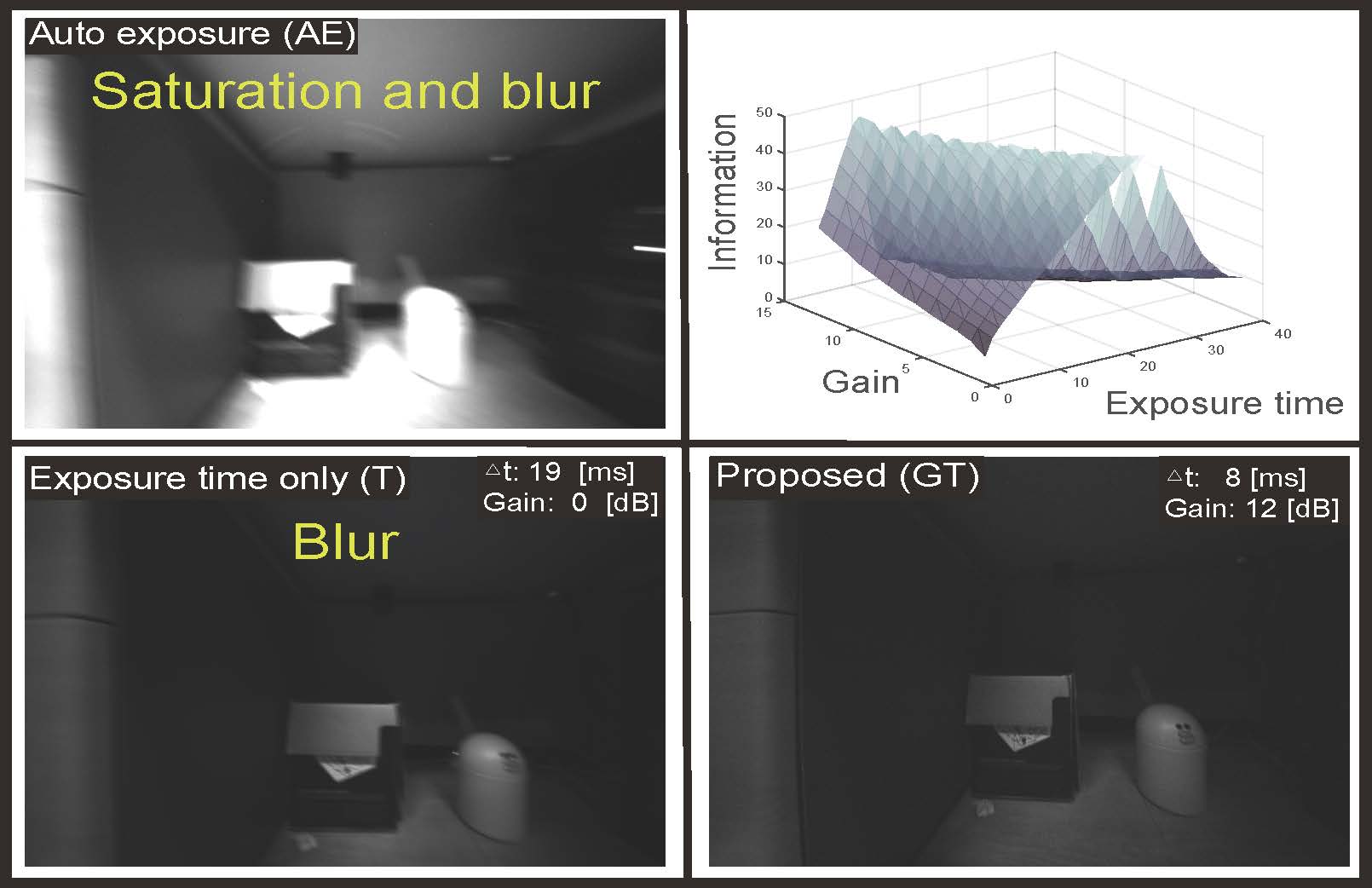
In conventional approaches, the two attributes are considered in a passive manner. For exposure time selection, many vision-based approaches rely on either automatic exposure control built into the camera or a fixed exposure value assuming a constant brightness in an environment. For the choice of gain, the increase of the gain was prohibited to avoid noisy images. But most critically, the two attributes were tackled separately.

Figure 2: Diagram for the proposed method. The overall procedure consists of four modules, (i) image synthesis, (ii) metric evaluation, (iii) metric compensation and (iv) control module.

Simultaneous control of these two attributes is beneficial in many aspects. When the camera undergoes extreme light condition, careful gain control is essential. For a dark scene, meaningful camera control is possible only when the gain partakes. Our finding is that the two parameters are closely related as in Fig. 1 and an unified controller needs to solve for the optimal attribute in a generic manner.

In this paper, we extend our previous exposure control by associating it with camera gain control. The proposed method is novel presenting the following contributions:

• We present a generic approach for active camera attribute control by considering both exposure time and gain. While these two factors are often determined separately, we report a thorough experiments to analyze the associative effect of exposure time and gain under a light varying environment.

• The main limitation of our previous work [1] was at the cost of evaluating a function by capturing real images with a specific exposure time. We improve the acquisition module by introducing image synthesis. As a result, we achieved a substantial improvement in attribute control for performance.

II Related Works

Among the camera attribute capturing images, gain and exposure time controls were widely studied. Exposure control has been examined especially in the HDR environment. Early works on the HDR environment mostly intended to compensate the pixel loss from saturation by using a CRF

Image Fusion in HDR Debevec and Malik [4] defined the relationship between the CRF and radiance value through linear mapping and created a synthetically computed radiance map to reconstruct an HDR image that is suitable for human vision. In [5], the authors introduced the camera’s radiometric response function to a single grayscale image without using a registered set of images. Using the statistical properties of the grayscale histogram in the edge area, the authors obtained information about the radiometric calibration.

Exposure time control In recent years, research has been conducted on finding appropriate exposure times in the robotics field [2], [3], and [6]. Shim [2] proposed using a method that selects the exposure time of a camera by examining the largest gradient magnitude of an image. The synthetic images were generated using a gamma function and mapped to the exposure time. Zhang [3] used the gradient percentile to express the image information amount by weighting the gradient. They also examined a photometric response function to control the exposure time. Another method [6] is to leverage image entropy to measure the amount of information in an image and adjust the exposure time and gain accordingly. By doing so, the image parameter with the highest entropy is selected while no control scheme was considered.

Gain control AGC (AGC) is a camera function that increases the average gain when the image is too dark and reduces it when the image is too bright [7]. In order to prevent the gain from oscillating, the increase and decrease of the gain between adjacent frames is limited to one. Litvinov and Schechner [8] proposed a solution that utilizes a radiometric response function to simultaneously estimate the unknown response function and camera gain (exposure) in the image sequences.

III Generic Camera Attribute Control

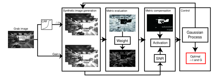
We now introduce a generic camera attribute controller that simultaneously controls both gain and exposure time. The overall process is as shown in Fig. 2. Results from an improper assignment of these two attributes are critical. The improper exposure time may blur and saturate the resulting images; change in gain produces additional noise when a higher gain is applied. To properly handle these factors, we modified our previous image quality evaluation metric to include the noise caused by gain control.

III-A Image Information Measure using SNR

Let us start with the image quality evaluation metric. We variate from the metric introduced in our previous work [1] to include not only saturation from exposure but also noise from an increase in gain. For an image $I$, the proposed evaluation metric $G_{I}$ is the summation of metric from the exposure time $(G_{t})_{I}$ and metric from the gain $(G_{k})_{I}$

$$G_{I}=(G_{t})_{I}-\frac{1}{\kappa}(G_{k})_{I}$$ (1)

, where $\kappa$ is the user parameter controlling the penalization balance between the exposure time and the gain. In this work $\kappa=5$ was used. The computed metric is then compensated using a saturation mask and activation function. We adopted our previous module for this compensation [1].

The first term, $(G_{t})_{I}$, is the EWG (EWG) from our previous work [1]. For a pixel $i$, we compute $(g_{t})_{i}$ using magnitude of gradient $\parallel\nabla I(i)\parallel^{2}$, entropy $H_{I}$, activation function $\pi(\cdot)$, image mask $M_{i}$, and entropy weight $W_{i}$ as below.

$$\scriptsize(g_{t})_{i}=W_{i}\parallel\nabla I(i)\parallel^{2}+\pi(H_{i})M_{i}(H_{i})W_{i}\frac{1}{N}\sum_{j=0}^{N-1}\parallel\nabla I(j)\parallel^{2}$$ (2)

The overall EWG for entire image $I$ is the summation of $g_{i}$ over $N$ pixels $(G_{t})_{I}=\sum_{i}^{N}(g_{t})_{i}$. This EWG consists of a term for image gradient and a term for saturation penalty. We refer to our previous derivation in [1] for detail of each term.

When taking gain into consideration, we need to account for the subsequent increase in noise. To incorporate the increase in noise, we adopted a SNR (SNR) as a physical measure of sensitivity to noise. The SNR of an image is typically calculated as the ratio of the mean pixel to the standard deviation of the pixel for a given neighbor. In general, the lower the gain, the higher the SNR and the better the image quality. We propose including this SNR in the image evaluation metric to penalize the increase of noise by the gain. Industry standards measure and define sensitivity in terms of the ISO film; $32\text{\,}\mathrm{d}\mathrm{B}$ is defined as an excellent image quality and $20\text{\,}\mathrm{d}\mathrm{B}$ as an acceptable image [9]. In this paper, we weight the image gradient using an SNR ratio with respect to this acceptable $SNR_{ref}=20$. We compute $(g_{k})_{i}$ for each pixel $i$ as

$$\small(g_{k})_{i}=\left(1-\frac{SNR}{SNR_{ref}}\right)\left(\frac{1}{N}\sum_{j=0}^{N-1}\parallel\nabla I(j)\parallel^{2}\right).$$ (3)

Then, the SNR metric for entire image $I$ is the summation of $(g_{k})_{i}$ over $N$ pixels $(G_{k})_{I}=\sum_{i}^{N}(g_{k})_{i}$.

Given two terms for exposure time $(G_{t})_{I}$ and gain $(G_{k})_{I}$, we sum two terms as in (1). We will denote this final metric, $G_{I}$, as NEWG (NEWG) throughout the paper.

III-B Camera Attribute Control

(a) True distribution

(b) Estimated distribution

Figure 3: Example of camera attribute control. 3(a) True distribution of NEWG and true optimal values (blue circle). 3(b) Estimated distribution using training points (red x) and predicted optimal values (blue circle).

Using a metric that accounts for both exposure time and gain, we perform attribute control by using Bayesian optimization. Because NEWG analyzes pixel distribution, which requires high levels of computation, we apply a GP (GP)-based optimization strategy to predict the best parameter for each attribute. Our control module, an extension of our previous work [1], jointly estimates the best exposure and gain values for next image input.

We select stationary and simple kernel function, SE (SE). For our application, the query exposure and gain spaces are bound by minimum and maximum exposure and gain values. After restricting the input space of our control parameters, we estimate optimal and fixed hyper-parameters via a log-likelihood optimization technique. To derive varying hyper-parameters, we construct various training datasets (exposure, gain and relative metrics) on several environments.

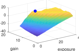
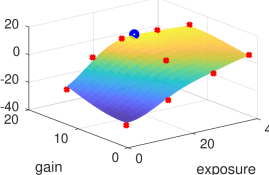
For camera attribute control, we use incremental learning with a maximum variance acquisition function [1]. Until termination conditions, the camera’s parameters are iteratively estimated as an exploration task. Fig. 3 represents a true NEWG distribution Fig. 3(a) and estimated with the selected query points Fig. 3(b). As described in the figure, the optimal parameters are well-estimated as the ground truth values.

IV Synthetic Image Generation

Next, we evaluate two different camera attributes and their subsequent increase in burden on capturing an image. In our previous approach [1], the function evaluation in Bayesian optimization corresponds to an actual frame acquisition. Despite the reduced function evaluation in using Bayesian optimization, image acquisition may slow down when a longer exposure time is applied. To mitigate the cost in the image grab, we propose using synthesized images instead of capturing images by assigning a target gain value and exposure time. Image synthesizing was introduced by Shim [2] who generated a synthetic image using gamma correction, which transforms image intensity using a nonlinear transfer function. This synthesis, which is based on a gamma function, is oriented to generate a natural scene for human vision and may not be fully realistic.

In this section, we introduce image synthesizing for a target exposure time and gain value. Specifically, we determine two scale factors $K_{t}$ (for exposure time) and $K_{g}$ (for gain) to be multiplied to the seed image when generating a synthetic image. Note that our objective was not to generate realistic image but to evaluate the NEWG score of the synthetic image. To leverage the computational speed, we synthesized the image from a down-sampled seed image by multiplying the scale factor $K_{synth}$, which is a combination of $K_{t}$ and $K_{g}$. For the scaling factor associated with exposure time, we use CRF and assume a constant irradiance at image acquisition. The scaling factor regarding gain is rather straightforward in that we can derive the factor directly from gain.

IV-A Image Synthesizing using CRF

We start with revisiting CRF from machine vision research. The CRF represents the relationship between the sensor irradiance of the camera and the measured intensity. In the field of computer vision, research has been conducted on estimating the CRF to achieve a high dynamic range image. Assuming that the CRF is spatially uniform within an image, the CRF can be widely estimated from the same set of images with different but known exposures [5], [4], and [10]. Among the existing methods, we focus on CRF estimation by [4], who expressed the nonlinear relationship of the CRF as

$$I_{x}=f(E_{x}\Delta t)$$ (4)

, where $I_{x}$ is the measured intensity level at the pixel location $x$, $E_{x}$ is the irradiance of the image at a pixel location $x$, $\Delta t$ is exposure time.

Note that our objective is to quickly generate synthetic images for an optimal camera attribute search, not to generate the most similar synthetic images to real. In that sense, we further simplified (4) by averaging over the entire image as

$$I=f(E\Delta t).$$ (5)

$E$ is now the average irradiance of the image. Although this CRF is unknown, we do know it is monotonic and continuous. Using this function property, many HDR imaging research studies [11] focus on the inverse of CRF (5), called an inverse response function for fitting and image synthesizing. The inverse CRF is in a log form and is a function of irradiance and exposure time as equation below.

$$g(I)=\ln(E\Delta t).$$ (6)

(a) Inverse CRF fitting

(b) Synthesizing scale

Figure 4: The example of inverse camera RF for exposure time. The intensity is evaluated over randomly sampled pixel points.

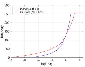
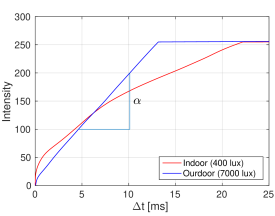
Following [4], two image acquisitions fully determines this inverse CRF. Furthermore, these acquisitions are readily available via an initial function evaluation for Bayesian optimization. To exploit the function, we need to determine the overall irradiance applied to an image $(E)$ for exposure time respectively by fitting the data to (6). We follow the same procedure introduced in [4]. Unlike conventional methods that evaluate RF over a series of images to exactly fit the function in (4), our focus is to find $E$ and fit the RF quickly, so as to be used in image synthesis corresponding to arbitrary camera attributes. For this purpose, we fit the inverse CRF using two sample points at the boundary. For example, minimum and maximum exposure time are evaluated to generate two samples for the fitting. A sample fitted graph on exposure time is shown in Fig. 4.

Fig. 4 presents a fitted inverse CRF for two different irradiance values (i.e., indoor and outdoor). The shape changes as the irradiance changes. Plotting intensity $g(I)$ with respect to $E\Delta t$ and removing log reveals a locally linear characteristic of the function as shown in Fig. 4(b). Our scaling factor is motivated by this plot and [11]. In [11], authors computed a synthetic image at a target exposure time $(\Delta t_{2})$ using an obtained image at the current exposure time $(\Delta t_{1})$, inverse CRF and the ratio between $\Delta t_{1}$ and $\Delta t_{2}$. When we know the ratio $\gamma=\Delta t_{2}/\Delta t_{1}$, image intensity corresponds to $\Delta t_{2}$ becomes

$$I_{\Delta t_{2}}=g^{-1}\left(\gamma g(I_{\Delta t_{1}})\right)=g^{-1}(\gamma g(\ln E+\ln\Delta t_{1})).$$ (7)

Using this intensity relation, for target exposure time $\Delta t_{s}$, we determine scale factor $K_{t}$ to be applied for each pixel of the seed image ($I_{o}$) captured with the seed exposure time $(\Delta t_{o})$. Using at least two real images obtained, we fit the inverse CRF and compute the intensity ratio from the plot as in Fig. 4(b). Assuming the irradiance ($E$) of the image is constant, the intensity ratio can be used to predict the average intensity of the synthesized image $I_{s}$ as

$$\alpha = \frac{g(I_{s})-g(I_{o})}{\Delta t_{s}-\Delta t_{o}}$$ (8)

$$K_{t}=\frac{g(I_{s})}{g(I_{o})} = \frac{\alpha(\Delta t_{s}-\Delta t_{o})+g(I_{o})}{g(I_{o})}$$ (9)

, where $g(I_{s})$ is the average intensity of the synthesized image found in the inverse CRF function. Once fitted with an inverse CRF, the scaling factor $K_{t}$, which is associated with exposure time is directly obtained.

(a) Indoor ($400\text{\,}\mathrm{l}\mathrm{u}\mathrm{x}$)

(b) Outdoor ($7000\text{\,}\mathrm{l}\mathrm{u}\mathrm{x}$)

Figure 5: The average image intensity of the real and synthetic image are plotted while changing the gain. Images are synthesized via (10) by using the image intensity captured in $0\text{\,}\mathrm{d}\mathrm{B}$ as the seed image ($I_{o}$).

Illuminance [lux]		10	50	80	100	320	400	1000
Environment		Dark scene	Living room	Hallway	Overcast	Office	Sunny	Artificial light
SNR-ignored	$\Delta t^{*}$ [ms]	17.0	12.0	5.5	5.5	2.5	2.0	2.0
(EWG)	$G^{*}$ [dB]	11	3	0	0	11	4	1
SNR-considered	$\Delta t^{*}$ [ms]	19.5	12.5	5.5	5.0	7.0	2.0	1.5
(NEWG)	$G^{*}$ [dB]	9	0	0	0	1	4	1

(a) Comparison of optimal parameters

(b) Camera rig

Figure 6: 6(a) comparison of optimal parameters ($\Delta t^{*}$ and $G^{*}$) depending on the choice of metric (i.e., SNR-ignored (EWG) vs. SNR-considered (NEWG)). 6(b) A multi camera rig and a light meter used in the test. Each camera operates controller using gain and $\Delta t$ (GT), auto exposure (AE), and exposure time only (T) respectively.

IV-B Image Synthesizing for Gain

Determining scale factor $K_{g}$ for gain is straightforward using the definition for the gain, $g=20\log_{10}\frac{g(I_{s})}{g(I_{o})}$. Because we wish to synthesize an image with gain factor $K_{g}$, the above equation can be further simplified as

$$g(I_{s})=K_{g}g(I_{o})=(10/F_{n})^{\frac{g}{20}}g(I_{o})\simeq 7.01^{\frac{g}{20}}g(I_{o})$$ (10)

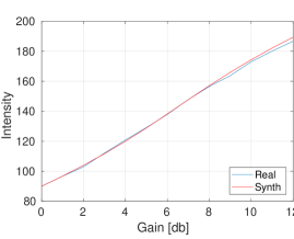
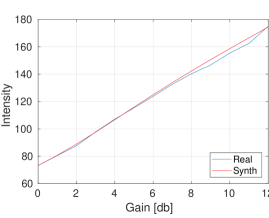
Factoring with $F_{n}=\sqrt{2}$ was empirically determined. For indoor and outdoor evaluation dataset, we plotted the average intensity of both real and synthetic images by varying gain as in Fig. 5. As can be seen in the figure, the scaling factor successfully captures the average image intensity for both indoor and outdoor settings.

V Experiments

To evaluate the proposed metric and image synthesis capability, we performed an exhaustive evaluation of data collection in various light conditions. The summary of the data is provided in the table in Fig. 6(a). This image synthesizing is included into our control scheme to produce a fast evaluation for optimal camera attribute control.

V-A Validation of Image Evaluation Metric

We first validate the image evaluation metric by comparing our previous metric against the proposed metric that additionally considers the SNR. When gain is simultaneously controlled with exposure time, the SNR affects image quality and should be incorporated into the metric.

In various illumination conditions, we collected an exhaustive dataset to validate our metric and image synthesis quality. We captured actual images while changing exposure time from $1\text{\,}\mathrm{m}\mathrm{s}$ to $20\text{\,}\mathrm{m}\mathrm{s}$. For this test, this range was selected because the image blurs when the exposure time is too large. Similarly, actual images with various gain values were obtained by changing the gain values from $0\text{\,}\mathrm{d}\mathrm{B}$ to $12\text{\,}\mathrm{d}\mathrm{B}$. For each pair of exposure time and gain, an image was captured and an associated metric was evaluated.

(a) 10 lux

(b) 320 lux

(c) 1000 lux

(d) 10 lux

(e) 320 lux

(f) 1000 lux

Figure 7: Sample image evaluation metric plotted with respect to the gain and exposure time. Top row depicts the metric when only considering saturation and the bottom row represents the metric when both saturation and the SNR. The red dot represents the optimal value of each metric. Note the change in the optimal values for 320 lux when SNR is additionally considered.

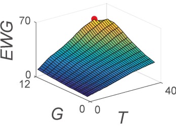
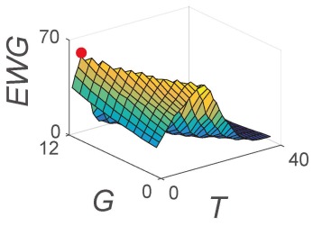
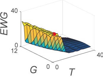
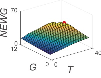
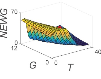
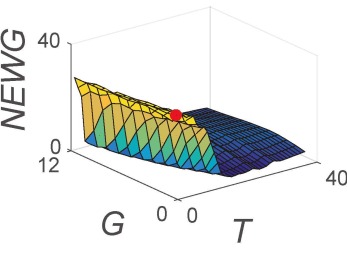
Fig. 7 compares two different metrics while changing exposure time and gain exhaustively. The newly proposed SNR-considering metric (bottom row) was plotted in comparison to a metric that does not consider the SNR (top row). Unlike the metric without the SNR in our earlier work [1], the new metric effectively compensates for noise even in dark environments. As can be seen in the dark case (10 lux), the overall curve of the graph increases less drastically with the new metric (Fig. 7(d) and Fig. 7(a)). By including noise into the metric, higher exposure and gain are less favored by the penalty from the increase in noise. The previous metric heavily aimed to eliminate saturation areas in the images (e.g., windows) obtained from an office environment (320 lux). However, the new metric was willing to tolerate saturation provided that no higher noise is yielded in the images (Fig. 7(e)). In addition, this metric prevents the image from creating an excessively high gain, even in a bright environment that can be sufficiently controlled by exposure time only. On the other hand, there is little effect in very bright environments ($1000\text{\,}\mathrm{l}\mathrm{u}\mathrm{x}$). This is because our algorithm searches for the balanced exposure time and gain. In a dark environment, the image quality is hardly controlled only by the exposure time control.

Table in Fig. 6(a) lists the optimal exposure time and optimal gain for each environment determined by two metrics. As can be seen in the table, the SNR-considered metric penalized the gain values effectively, preventing an optimal high gain value to be reached. For example, when the environment is fairly bright ($320\text{\,}\mathrm{l}\mathrm{u}\mathrm{x}$), images with a low exposure time ($2.5\text{\,}\mathrm{m}\mathrm{s}$) but high gain ($11\text{\,}\mathrm{d}\mathrm{B}$) were preferred because they contained more gradients despite the increased noise. On the other hand, when the SNR is considered, this issue is alleviated by selecting a larger exposure time ($7.0\text{\,}\mathrm{m}\mathrm{s}$) and low gain ($2\text{\,}\mathrm{d}\mathrm{B}$). As similar improvement was found when the environment was dark ($10\text{\,}\mathrm{l}\mathrm{u}\mathrm{x}$) forcing the optimal value to occur with a lower gain value.

(a) Indoor evaluation. The figures show images obtained at different exposure times in $1\text{\,}\mathrm{m}\mathrm{s}$ intervals during the day (left top), images measured differently in $1\text{\,}\mathrm{d}\mathrm{B}$ intervals (right top), and synthetic images corresponding to those images (bottom).

(b) Outdoor evaluation. The figures show images obtained at different exposure times in $5\text{\,}\mathrm{u}\mathrm{s}$ intervals during the day (left top), images measured differently in $1\text{\,}\mathrm{d}\mathrm{B}$ intervals (right top), and synthetic images corresponding to those images (bottom).

Figure 8: Synthesized image evaluation. Comparing and analyzing synthetic image for camera gain and synthetic image for exposure time using camera response function. The red box is the image with the maximum amount of information (NEWG) in the actual image, and the blue box is the image that shows the maximum amount of information in the synthetic image.

V-B Validation of Image Synthesis

(a) Indoor test

(b) Outdoor test

Figure 9: For both indoor and outdoor tests, each row represents an acquired image that was controlled for automatic exposure (AE), exposure time (T), and exposure time and gain (GT). 9(a) The experiment was conducted in an indoor environment at night. Exposure time (in ms) and gain (in dB) are marked in the top right corner of each image. During the drastic change between ‘B’ and ‘C’, AE resulted in saturation for a bright scene (‘C’) by focusing on the exposure for the dark scene in (‘B’). Exposure-only control was insufficient to overcome the dark scene (‘B’). 9(b) The experiment was conducted in an outdoor environment after sunset. Large exposure time for a dark scene was not sufficient for AE and T. Due to this limited light, motion blur and high noise occurred.

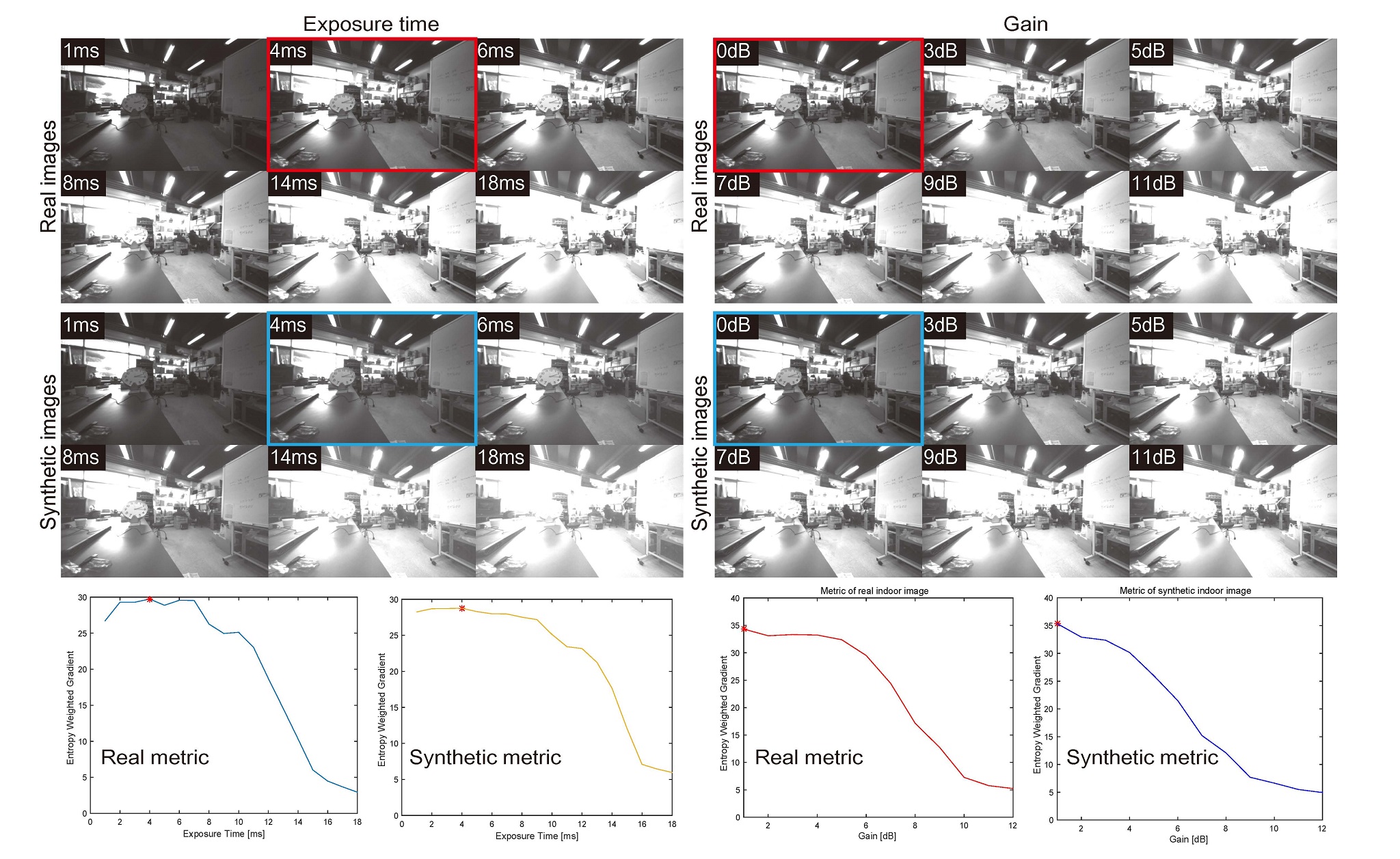
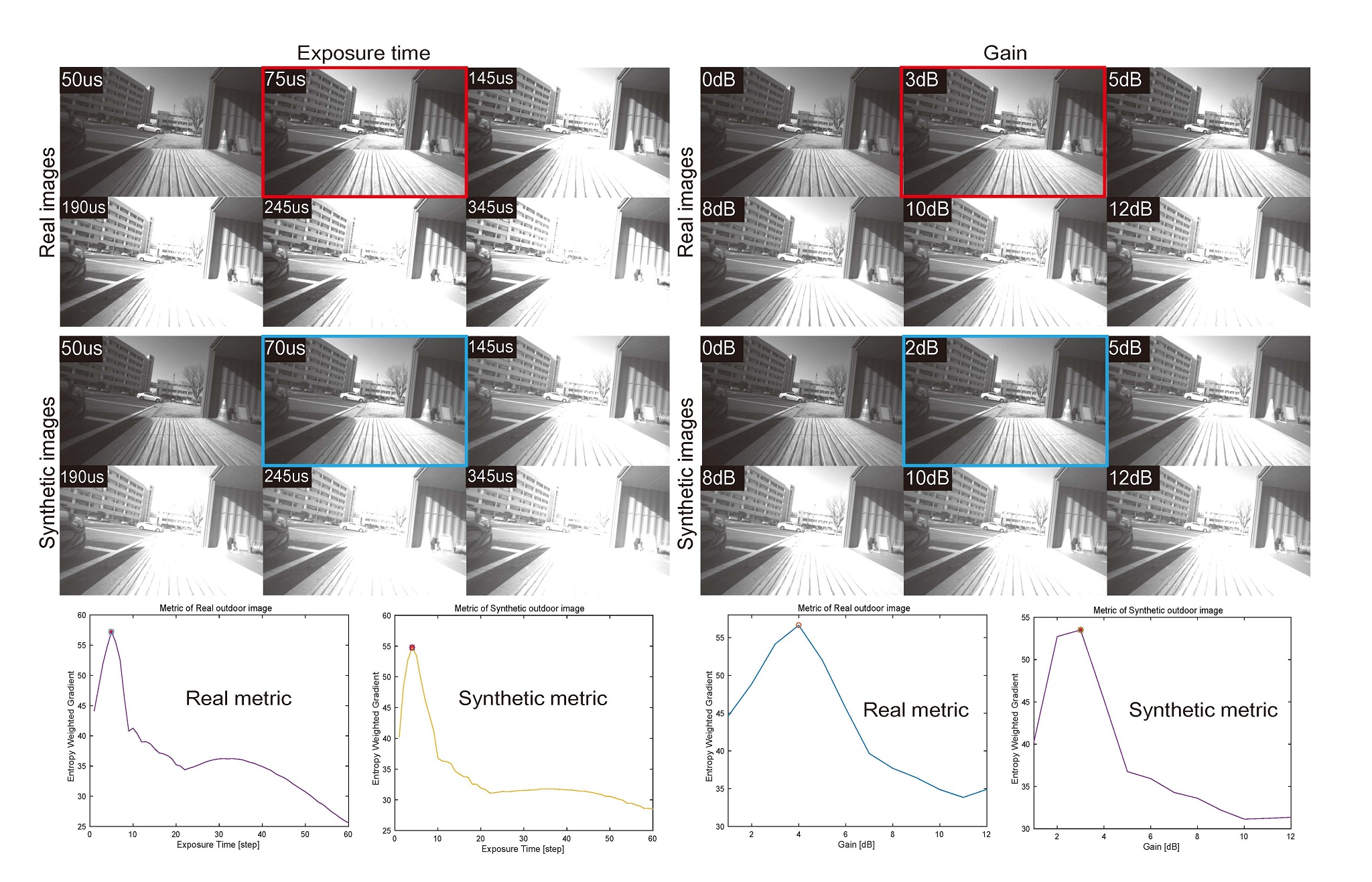
Before applying the synthetic image in our control loop, we validated the effectiveness of the proposed image synthesis by comparing them with the real images, which was captured while varying exposure and gain respectively. Using these actual images as a baseline (top group in Fig. 8(a) and Fig. 8(b)), we synthesized the images for the intended exposure time and gain values (bottom group in Fig. 8(a) and Fig. 8(b)). For the exposure time based synthesis, we used the seed image with a minimum exposure time ($1\text{\,}\mathrm{m}\mathrm{s}$) to generate other images. For the gain based synthesis, we used zero gain ($0\text{\,}\mathrm{d}\mathrm{B}$) image as the seed image.

We conducted more quantitative analysis by plotting the image quality metric variation. We measured the proposed image metric from both synthetic and real images. We would like to stress that our intention was not to synthesize an image to be the same as a real image. Rather, we intend to achieve an image synthesis process that follows a similar metric evaluation. As shown in the metric plots in Fig. 8(a) and Fig. 8(b), the resulting synthesized image sequence revealed the similar image evaluation metric when compared to the metric obtained from the real image sequence. Most importantly, the selected optimal value is the same for both the synthetic and real image sequences, thus proving that the proposed synthetic images can be used to find the optimal camera attribute.

V-C Camera Attribute Control

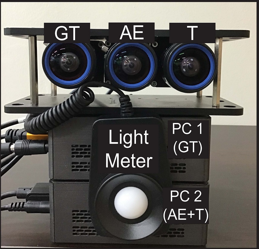
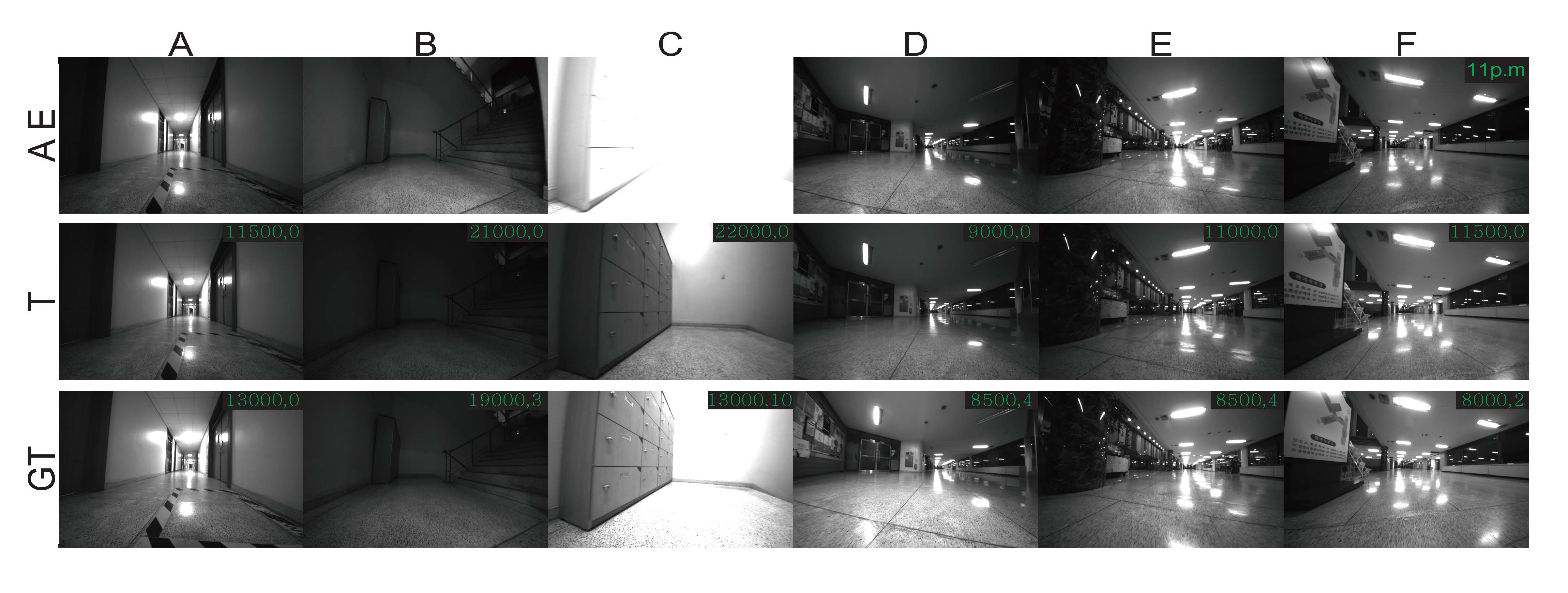
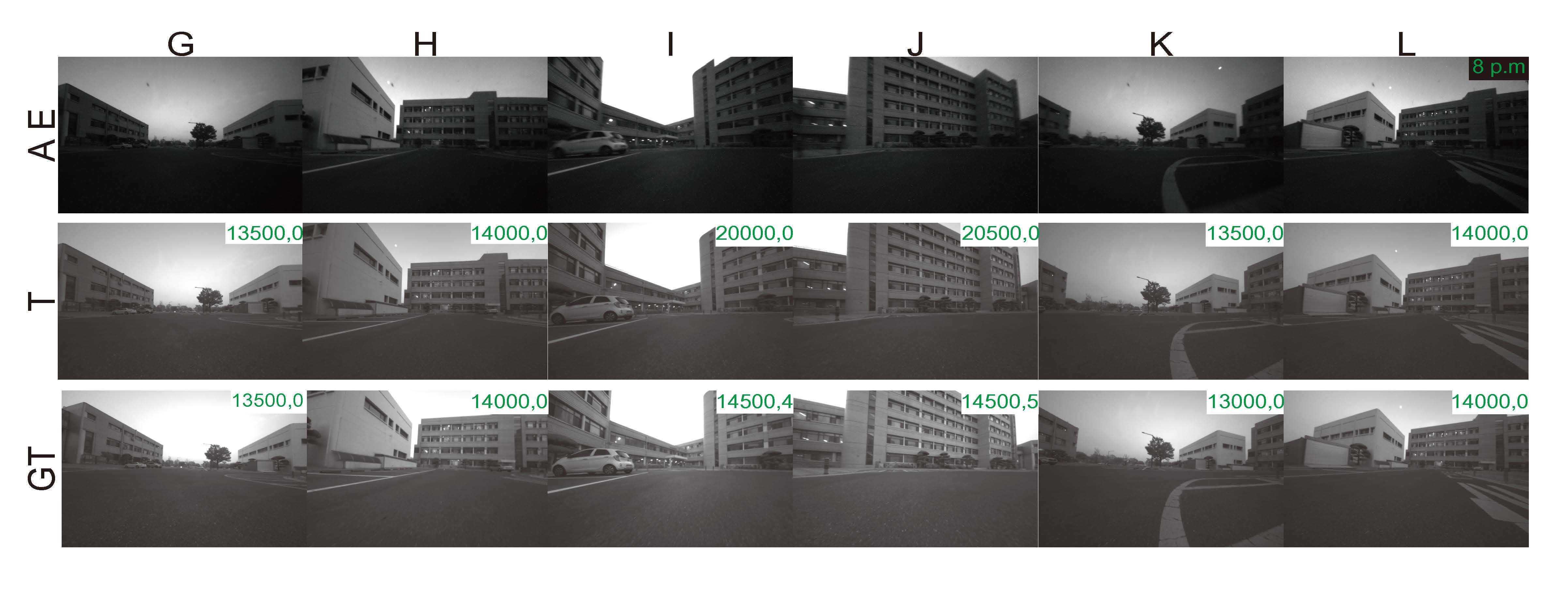
Next, we present experimental validation in both indoor and outdoor environments. For both tests, three cameras are mounted as in Fig. 6(b). For indoor validation, the test was performed in an indoor corridor at night, where the light was automatically controlled by passenger motion. As the robot moved, the light turned on and off repeatedly. For outdoor validation, images were captured right after sunset when the light is limited.

Fig. 9 summarizes the experimental results from the indoor environment. When the exposure was controlled automatically (AE), too large exposure time was assigned for a dark scene, and producing an over-exposed image in the upcoming frame (first row, B and C). If we only control exposure time as in our previous study, an under-exposed image occurred in dark environments (second row, B). Similarly for outdoor, Fig. 9(b) shows an outdoor environmental experiment right after sunset. As it became dark, the auto attribute control (AE) yielded images with high noise by assigning a high gain value. Furthermore, lack of light and the large exposure resulted in a motion blur. For both experiments, the proposed camera attribute control simultaneously controls gain and exposure time to prevent motion blur and saturation in the entire image.

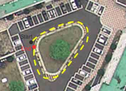
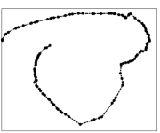
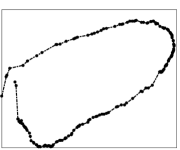
We also verified the proposed method in a SLAM (SLAM) framework, we piped the acquired images in the ORB SLAM [12] (Fig. 10). In both cases when using automatic exposure control and exposure time-only control, tracking failure was caused by under-exposure. Refer to attached multimedia gcac.mp4 for more detailed tracking results. For the outdoor test, automatic attribute control failed even at the initialization phase. Similar to the indoor setting, handling gain and exposure time together (Fig. 10(c)) outperformed exposure time only control (Fig. 10(b)), resulting in the more consistent trajectory.

V-D Discussion on Optimal Attribute and Computational Cost

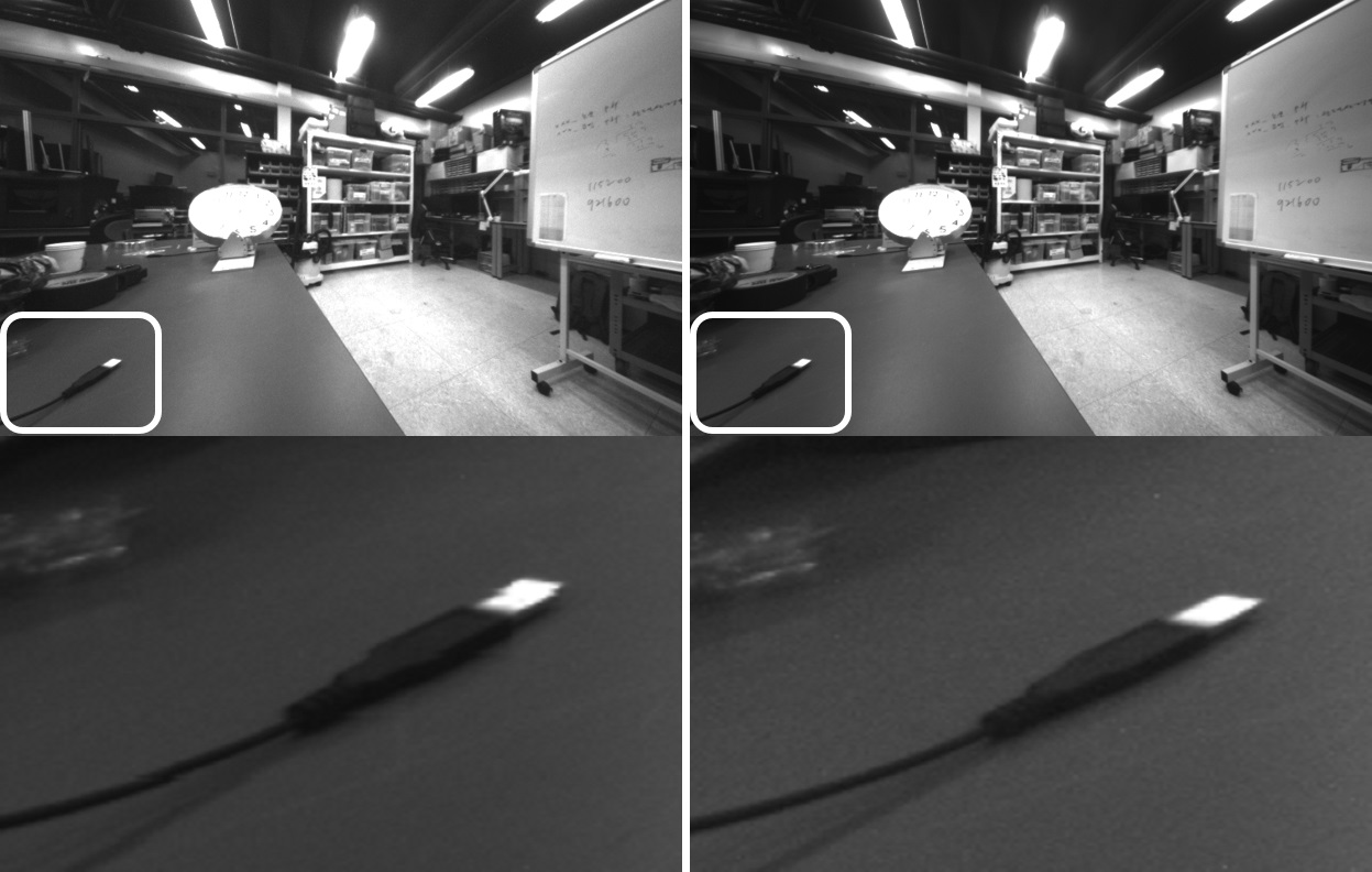
Selecting the optimal camera attribute is critical especially when light conditions change in a dark environment. Fig. 11 depicts two sample images taken from different attribute pair. As can be seen in the zoomed view, the noise level is substantially higher when high gain is assigned. This indicates the importance of the joint control of the camera attributes.

(a) Trajectory

(b) $\Delta{t}$ control

(c) $\Delta{t}$ and Gain control

Figure 10: Trajectory of ORB SLAM in outdoor environment. The automatic attribute control (AE) caused noisy images from high gain and the ORB SLAM failed at the initialization phase, and thus excluded in the plot.

Figure 11: The left image is high exposure time and low gain, the right image is low exposure and high gain image

Overall, our algorithm updates the exposure parameter to $10\text{\,}\mathrm{H}\mathrm{z}$. Using a synthetic image for function evaluation substantially improve the performance and ensure a real-time image stream. The detailed timing for each module is summarized in the Table. I.

TABLE I: Time required per each module

Module	Img. Synth.	Metric eval.	Total Control
	[ms]	[ms]	[ms]	[Hz]
10 lux	0.254	13.780	101.278	9.87
320 lux	0.247	12.768	94.215	10.61
1000 lux	0.246	13.242	93.364	10.71

VI conclusion

This paper reported generic camera attribute control for both exposure time and gain. The proposed control scheme simultaneously controls exposure time and gain using fast function evaluation from CRF based image synthesis. To the best of our knowledge, the proposed method is the first unified and generic approach to control exposure time and gain at the same time. We provided extensive evaluations to discuss the relation between these two attributes in the resulting images.

References

- Kim et al. [2018] J. Kim, Y. Cho, and A. Kim, “Exposure control using bayesian optimization based on entropy weighted image gradient,” in Proc. IEEE Intl. Conf. on Robot. and Automat., 2018, in print.
- Shim et al. [2014] I. Shim, J.-Y. Lee, and I. S. Kweon, “Auto-adjusting camera exposure for outdoor robotics using gradient information,” in Proc. IEEE/RSJ Intl. Conf. on Intell. Robots and Sys., 2014, pp. 1011–1017.
- Zhang et al. [2017] Z. Zhang, C. Forster, and D. Scaramuzza, “Active exposure control for robust visual odometry in hdr environments,” in Proc. IEEE Intl. Conf. on Robot. and Automat., no. EPFL-CONF-228466, 2017.
- Debevec and Malik [1997] P. E. Debevec and J. Malik, “Recovering high dynamic range radiance maps from photographs,” in Proc. of the conf. on Comput. graph. and inter. tech., 1997, pp. 369–378.
- Lin and Zhang [2005] S. Lin and L. Zhang, “Determining the radiometric response function from a single grayscale image,” in Proc. IEEE Conf. on Comput. Vision and Pattern Recog., vol. 2, 2005, pp. 66–73.
- Lu et al. [2010] H. Lu, H. Zhang, S. Yang, and Z. Zheng, “Camera parameters auto-adjusting technique for robust robot vision,” in Proc. IEEE Intl. Conf. on Robot. and Automat., 2010, pp. 1518–1523.
- Fowler [2004] K. R. Fowler, “Automatic gain control for image-intensified camera,” IEEE Trans. Instrum. and Meas., vol. 53, no. 4, pp. 1057–1064, 2004.
- Litvinov and Schechner [2005] A. Litvinov and Y. Y. Schechner, “Addressing radiometric nonidealities: A unified framework,” in Proc. IEEE Conf. on Comput. Vision and Pattern Recog., vol. 2, 2005, pp. 52–59.
- Yang and El Gamal [1999] D. X. Yang and A. El Gamal, “Comparative analysis of snr for image sensors with enhanced dynamic range,” in Sen, Cam, and Sys. for Sci/Indu. App., vol. 3649, 1999, pp. 197–212.
- Ng et al. [2007] T.-T. Ng, S.-F. Chang, and M.-P. Tsui, “Using geometry invariants for camera response function estimation,” in Proc. IEEE Conf. on Comput. Vision and Pattern Recog., 2007, pp. 1–8.
- Grossberg and Nayar [2003] M. D. Grossberg and S. K. Nayar, “Determining the camera response from images: What is knowable?” IEEE Trans. Pattern Analysis and Machine Intell., vol. 25, no. 11, pp. 1455–1467, 2003.
- Mur-Artal et al. [2015] R. Mur-Artal, J. M. M. Montiel, and J. D. Tardos, “Orb-slam: a versatile and accurate monocular slam system,” IEEE Trans. Robot., vol. 31, no. 5, pp. 1147–1163, 2015.