Multi-Scale Gradual Integration CNN
for False Positive Reduction in Pulmonary Nodule Detection

Abstract

Lung cancer is a global and dangerous disease, and its early detection is crucial to reducing the risks of mortality. In this regard, it has been of great interest in developing a computer-aided system for pulmonary nodules detection as early as possible on thoracic CT scans. In general, a nodule detection system involves two steps: (i) candidate nodule detection at a high sensitivity, which captures many false positives and (ii) false positive reduction from candidates. However, due to the high variation of nodule morphological characteristics and the possibility of mistaking them for neighboring organs, candidate nodule detection remains a challenge. In this study, we propose a novel Multi-scale Gradual Integration Convolutional Neural Network (MGI-CNN), designed with three main strategies: (1) to use multi-scale inputs with different levels of contextual information, (2) to use abstract information inherent in different input scales with gradual integration, and (3) to learn multi-stream feature integration in an end-to-end manner. To verify the efficacy of the proposed network, we conducted exhaustive experiments on the LUNA16 challenge datasets by comparing the performance of the proposed method with state-of-the-art methods in the literature. On two candidate subsets of the LUNA16 dataset, i.e., V1 and V2, our method achieved an average CPM of 0.908 (V1) and 0.942 (V2), outperforming comparable methods by a large margin. Our MGI-CNN is implemented in Python using TensorFlow and the source code is available from https://github.com/ku-milab/MGICNN.

1 Introduction

Lung cancer is reported as the leading cause of death worldwide [41]. However, when detected at an early stage through thoracic screening with low-dose CT images and treated properly, the survival rate can be increased by 20% [27]. Clinically, pulmonary nodules are characterized as having round shape with a diameter of $3mm\sim 30mm$ in thoracic CT scans [12]. With this pathological knowledge, there have been efforts of applying machine-learning techniques for early and automatic detection of cancerous lesions, i.e., nodules. To our knowledge, a computerized lung cancer screening system consists of two-steps: candidate nodule detection and False Positives (FPs) reduction. In the candidate nodule detection step, the system uses high sensitivity without concern for specificity to extract as many candidates as possible. Roughly, more than 99% of the candidates are non-nodules, i.e., FPs [33], which should be identified and reduced in the second step correctly.

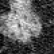
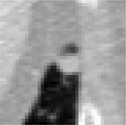
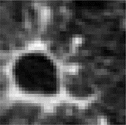
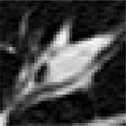
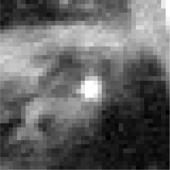
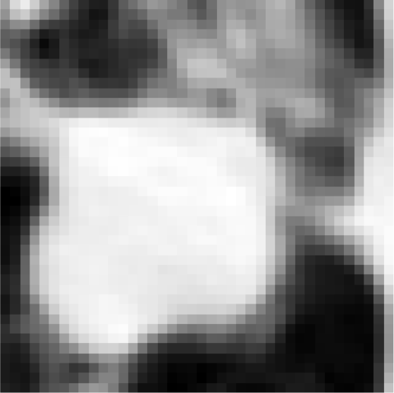
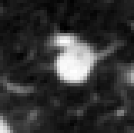
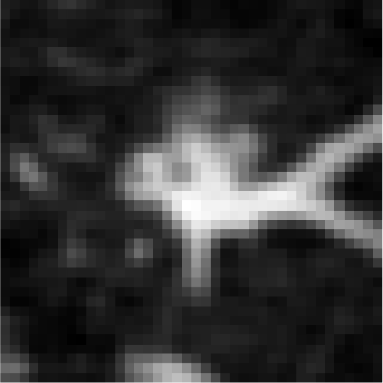
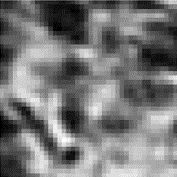
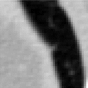
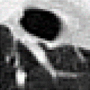
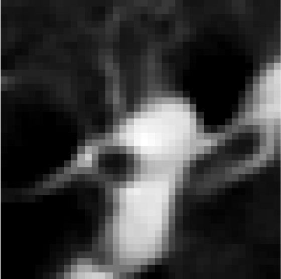
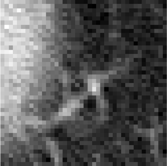
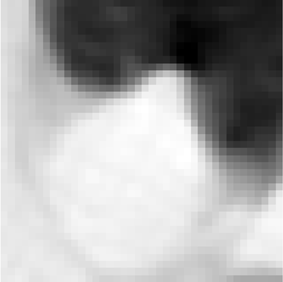
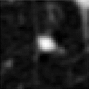
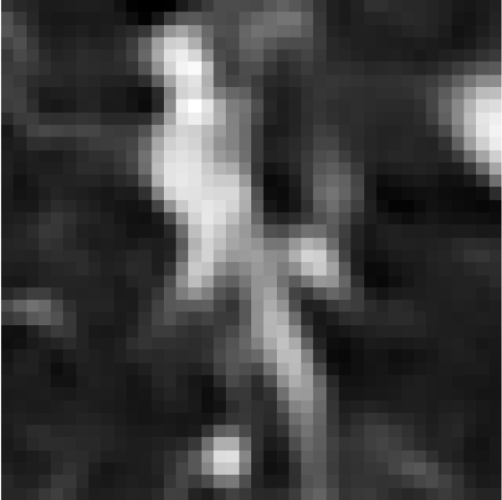
Pathologically, there are many types of nodules (e.g., solids, non-solids, part-solids, calcified, etc. [3]) and their morphological characteristics such as size, shape, and strength are highly variable. In addition, there are many other structure in the thorax (e.g., blood vessels, airways, lymph nodes) with morphological features similar to nodules [12, 31]. Fig. 1 shows an example of a nodule and a non-nodule. In these regards, it is very challenging to reduce FPs or to distinguish nodules from non-nodules, leading many researchers to devote their efforts on the step of false positive reduction [33, 6, 2].

(a) Nodule

(b) Non-nodule

Figure 1: Examples of the pulmonary nodules and non-nodules. Both have a complex and similar morphological characteristics that must be distinguished between.

In earlier work, researchers had mostly focused on extracting discriminative morphological features with the help of pathological knowledge about nodule types and applied relatively simple linear classifiers such as logistic regression or support vector machine [20, 29, 46]. Recently, with the surge of popularity and success in Deep Neural Networks (DNNs), which can learn hierarchical feature representations and class discrimination in a single framework, a myriad of DNNs has been proposed for medical image analysis [42, 7, 9, 13, 36, 16]. Of the various deep models, Convolutional Neural Networks (CNNs) have been applied most successfully for pulmonary nodule detection and classification in CT images [25, 17, 34, 33, 31, 24, 38]. Moreover, in order to attain the network performance of computer vision applications, there were trials [4, 40] to identify nodules with a deep model fine-tuned with pulmonary nodule data in the way of transfer learning [45, 30].

From previous studies of nodule detection or classification in CT scans, we have two notable findings. The first is that it is helpful to exploit volume-level information, rather than 2D slice-level information [31, 33, 5]. For example, Roth et al. [31] proposed a 2.5D CNN by taking three orthogonal 2D patches as input for volume-level feature representation. Setio et al. [33] proposed a multi-view CNN, which extracts hierarchical features from nine 2D slices with different angles of view, and groups the high-level features for classification. However, their method achieved limited performance in low-FP scans. Ding et al. [5] proposed a 3D CNN with a 3D volumetric patch as input, and presented promising results in FP reduction.

The second is that performance can be enhanced by using multi-scale inputs with different levels of contextual information [37, 6, 39]. Shen et al. [37] proposed a multi-scale CNN and successfully applied nodule classification by combining contextual information at different image scales with the abstract-level feature representations. Dou et al. [6] also designed a 3D CNN to encode multi-level contextual information to tackle the challenges of large variation in pulmonary nodules. The performance of pulmonary nodule classification using the 3D CNN is generally better than that of the 2D CNN [5]. However, the 3D CNN is more difficult to train than the 2D CNN due to the large number of network parameters. Medical image data is relatively limited, so a 3D CNN may easily become over-fitted. It is also noteworthy that the multi-scale methods have proved their efficacy in computer vision tasks [19, 14, 23].

Inspired by the above-mentioned findings, in this study we propose a novel Multi-scale Gradual Integration CNN (MGI-CNN) for FP reduction in pulmonary nodule detection. In designing our network, we apply three main strategies. Strategy 1: We use 3D multi-scale inputs, each containing different levels of contextual information. Strategy 2: We design a network for Gradual Feature Extraction (GFE) from multi-scale inputs at different layers, instead of radical integration at the same layer [19, 37, 39, 6]. Strategy 3: For better use of complementary information, we consider Multi-Stream Feature Integration (MSFI) to integrate abstract-level feature representations. Our main contributions can be summarized as follows:

1. We propose a novel CNN architecture that learns feature representations of multi-scale inputs with a gradual feature extraction strategy.

2. With multi-stream feature representations and abstract-level feature integration, our network reduces many false positives.

3. Our method outperformed state-of-the-art methods in the literature by a large margin on the LUNA16 challenge datasets.

While the proposed network architecture extension is straightforward, to our best knowledge, this is the first work of designing a network architecture that integrates 3D contextual information of multi-scale patches in a gradual and multi-stream manner. Concretely, our work empirically proved the validity of integrating multi-scale contextual information in a gradual manner, which can be comparable to many existing work [23, 18] that mostly considered radical integration of such information. Besides, our method also presents the effectiveness of learning feature representations from different orders of multi-scale 3D patches and combining the extracted features from different streams to further enhance the performance.

This paper is organized as follows. Section 2 introduces the existing methods in the literature. We then describe our proposed method in Section 3. The experimental settings and performance comparison with the state-of-the-art methods are presented in Section 4. In Section 5, we discuss key issues of the proposed method along with the experimental results. We conclude this paper by summarizing our work and suggesting the future direction for clinical practice in Section 6.

2 Related Work

2.1 Volumetric Contextual Information

Automatic lung cancer screening systems classify nodules using specific algorithms to extract nodule morphological characteristics. Okumura et al., [29] distinguished solid nodules by using a Quoit filter that could detect only isolated nodules. In the case of isolated nodules, the graph of the pixel values becomes ‘sharp,’ and the nodule is detected when the annular filter passes through the graph. However, filters that use only one characteristic of nodules have difficulty in distinguishing diverse nodule types. Li et al. [21] proposed point, line, and surface shape filters for finding nodule, blood vessel, and airway in a thoracic CT. This is a detection method that considers various types of nodules, effectively reducing the FP response of the automatic lung cancer screening system. However, hand-crafted features still do not detect complex types of nodules (e.g., part-solid or calcified nodules). Hence, to detect the more elusive types of nodule, researchers attempted to use volumetric information about the nodule and its surrounding area. Jacobs et al. [17] extracted volumetric information from various types of bounding boxes that defined the region around a nodule to classify part-solid nodules. That volumetric information includes 107 phenotype features and 21 context features of the nodule and various nodule area with diverse sizes of a bounding box. For the classification, the GentleBoost classifier [10] learned a total of 128 features and obtained 80% of sensitivity at 1.0 FP/scan. However, the method was inefficient in distinguishing the various types of nodule because it must be reconfigured to filter each nodule type.

Recently, DNNs have been successfully used to substitute the conventional pattern-recognition approaches that first extract features and then train a classifier separately, thanks to their ability of discovering data-driven feature representations and training a classifier in a unified framework. Among various DNNs, CNN-based methods reported promising performance in classifying nodules correctly. Roth et al. [31] proposed 2.5D CNN that used three anatomical planes (sagittal, coronal, and axial) to extract 3D nodule area volumetric information. Their 2.5D CNN also classified organs similar to nodules, such as lymph nodes. This study inspired some researchers in the field of pulmonary nodule detection. Setio et al. [33] proposed a multi-view CNN that extracted volumetric information with an increased number of input patches. Furthermore, to better consider contextual information, they used groupings of high-level features from each 2D CNN in a 9-view (three times more than 2.5D CNN’s anatomical plane) by achieving promising performance, compared with the methods using hand-crafted features. However, this effort could not fully utilize all the 3D volumetric information that could be useful to further enhance the performance. Ding et al. [5] tried to build a unified framework by applying a deep CNN for both candidate nodule detection and nodule identification. Specifically, they designed a deconvolutional CNN structure for candidate detection on axial slices and a three-dimensional deep CNN for the subsequent FP reduction. In the FP reduction step, they used a dropout method by achieving a sensitivity of 0.913 in average FP/scan on the LUNA16 dataset. Although they claimed to use 3D volumetric information, they did not consider the information between the small patches that were extracted in a large patch.

2.2 Multi-scale Contextual Information

From an information quantity perspective, it may be reasonable to use morphological and structural features in different scales and thus effectively integrating multi-scale contextual information. Shen et al. [37] proposed Multi-scale CNN (MCNN) as a method for extraction of high-level features from a single network by converting images of various scales to the same size. The high-level features are jointly used to train a classifier, such as support vector machine or random forest, for nodule classification. Dou et al. [6] used three different architectures of 3D CNN, each one of which was trained with the respective receptive field of an input patch empirically optimized for the LUNA16 challenge dataset. To make a final decision, they integrated label prediction values from patches of three different scales by a weighted sum at the top layers. However, the weights for each scale were determined manually, rather than learning from training samples.

Multi-crop Convolutional Neural Network (MC-CNN) to automatically extract nodule salient information by employing a novel multi-crop pooling strategy which crops different regions from convolutional feature maps and then applies max-pooling different times.

Shen et al. [39] proposed a Multi-Crop CNN to automatically extract nodule salient information by employing a novel multi-crop pooling strategy. In particular, they cropped different regions from convolutional feature maps and then applied a max-pooling operation different times. To give more attention on the center of the patches, they cropped out the neighboring or surrounding information during multi-crop pooling, which could be more informative to differentiate nodules from non-nodules, e.g., other organs.

In this paper, unlike the methods of [33, 31], we exploit 3D patches to best utilize the volumetric information and thus enhancing the performance in FP reduction. Further, to utilize contextual information from different scales, we exploit a multi-scale approach similar to [6, 39]. However, instead of radical integration of multi-scale contextual information at a certain layer [37, 39], we propose to gradually integrate such information in a hierarchical fashion. It is also noteworthy that we still consider the surrounding regions of a candidate nodule to differentiate from other organs, which can be comparable to [39].

(a) 3D Patch Extraction: Given the coordinates of a candidate nodule, we extract three patches in different scales and then resize them to the same size, i.e., $S1$, $S2$, and $S3$.

(b) Gradual Feature Extraction: The multi-scale patches with different levels of contextual information ($S1$-$S2$-$S3$ or $S3$-$S2$-$S1$) are integrated in a gradual manner.

(c) The architecture of the proposed multi-scale gradual integration CNN.

Figure 2: Overview of the propose framework for FP reduction in pulmonary nodule detection. The notations of $\|$ and $\oplus$ denote, respectively, concatenation and element-wise summation of feature maps. The numbers above the thick black or yellow arrows present a kernel size, e.g., $3\times 3$ and a stride, e.g., (1) and (2). (conv: convolution, MP: max-pooling)

3 Multi-scale Gradual Integration Convolutional Neural Network (MGI-CNN)

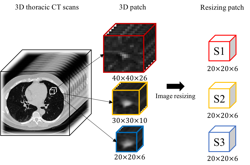
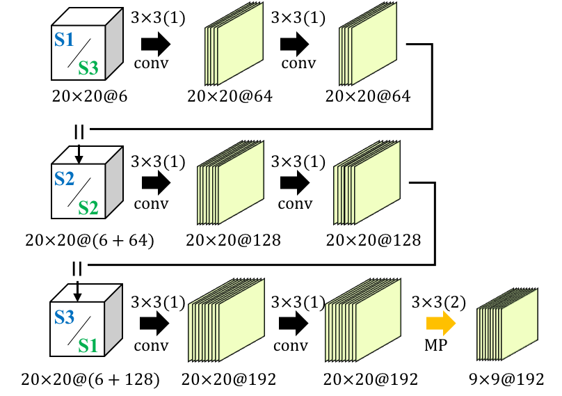
In this section, we describe our novel method of Multi-scale Gradual Integration Convolutional Neural Network (MGI-CNN) in Fig. 2 for pulmonary nodule identification, which consists of two main components: Gradual Feature Extraction (GFE) and Multi-Stream Feature Integration (MSFI). For each candidate nodule, we extract 3D patches at three different scales $40\times 40\times 26$, $30\times 30\times 10$, and $20\times 20\times 6$ by following Dou et al.’s work [6]. We then resize three patches to $20\times 20\times 6$, , denoted as $S1$, $S2$, and $S3$, respectively, as input to the proposed network (Fig. 2(a)). Note that patches of $S1$, $S2$, and $S3$ have the same center coordinates but pixels in the patches are different in resolution.

3.1 Gradual Feature Extraction

Inspired by the human visual system, which retrieves meaningful contextual information from a scene by changing the field of view, i.e., by considering contextual information at multiple scales [47], we first propose a scale-ordered GFE network presented in Fig. 2(b). In integrating morphological or structural features from patches at different scales, the existing methods [37, 39] combined features from multiple patches all at once. Unlike their methods, in this paper, we extract features by gradually integrating contextual information from different scales in a hierarchical manner. For gradual feature representation from multi-scale patches, i.e., $S1$, $S2$, and $S3$, there are two possible scenarios, i.e., $S1-S2-S3$ (‘zoom-in’) or $S3-S2-S1$ (‘zoom-out’).

For the zoom-in scenario of $S1-S2-S3$, a patch at one scale $S1$ is first filtered by the corresponding local convolutional kernels and the resulting feature maps $F1$ are concatenated ($\|$) with the patch at the next scale $S2$, i.e., $F1\|S2$. In our convolution layer, $F1$ is the result of two repeated computations of a spatial convolution and a non-linear transformation by a Rectifier Linear Unit (ReLU) [26]. Our convolution kernel uses zero padding to keep the size of the output feature maps equal to the size of an input patch and thus valid to concatenate the resulting feature maps and another input patch $S2$ in different scale. The $F1\|S2$ tensor is then convolved with kernels of the following convolution layers, producing feature maps $F12$, which now represent the integrated contextual information from $S1$ and $S2$. The feature maps $F12$ are then concatenated with the patch at the next scale $S3$ and the tensor of $F12\|S3$ is processed by the related kernels, resulting in feature maps $F123$. The feature maps $F123$ represent the final integration of various types of contextual information in patches $S1$, $S2$, and $S3$. The number of feature maps in our network increases as additional inputs are connected so that the additional information can be extracted from the information of the preceding inputs and the contextual information of the sequential inputs. For the zoom-out scenario of $S3-S2-S1$, the same operations are performed but with input patches in the opposite order.

In the zoom-in scenario, the network is provided with patches at an increasing scale. So, the field of view in a zoom-in network is gradually reduced, meaning that the network gradually focuses on a nodule region. Meanwhile, the zoom-out network has a gradually enlarging field of view, and thus the network finds morphological features combined with the neighboring contextual information by gradually focusing on the surrounding region. In our network architecture, the feature maps extracted from the previous scale are concatenated to the patch of the next scale with zero padding, and then fed into the following convolution layer. By means of our GFE method, our network sequentially integrates contextual features according to the order of the scales. It is noteworthy that the abstract feature representations from two different scenarios, i.e., zoom-in and zoom-out, carry different forms of information.

3.2 Multi-Stream Feature Integration (MSFI)

Rather than considering a single stream of information flow, either $S1-S2-S3$ or $S3-S2-S1$, it will be useful to consider multiple streams jointly and to learn features accordingly. With two possible scenarios of ‘zoom-in’ and ‘zoom-out’, we define the information flow of $S1-S2-S3$ as ‘zoom-in stream’ and the information flow of $S3-S2-S1$ as ‘zoom-out stream’.

As the zoom-in and zoom-out streams focus on different scales of morphological and contextual information around the candidate nodule in a different order, the learned feature representations from different streams can be complementary to each other for FP reduction. Hence, it is desirable to combine such complementary features in a single network and to optimize the feature integration from the two streams in an end-to-end manner. To this end, we design our network to integrate contextual information from the two streams as presented in Fig. 2(c) and call it as MSFI. The proposed MSFI is then followed by additional convolutional layers and fully-connected layers to fully define our MGI-CNN, as shown in Fig. 2(c).

Table 1: Statistics of the two datasets, i.e., V1 and V2, for FP reduction in the LUNA16 challenge. The numbers in parentheses denote the number of nodule-labeled candidates in each dataset that match with the radiologists’ decisions.

Dataset	Candidates
	Nodule	Non-nodule
V1	1,351 (1,120)	549,714
V2	1,557 (1,166)	753,418

4 Experimental Settings and Results

4.1 Experimental Settings

We performed the experiments on the LUng Nodule Analysis 2016 (LUNA16) challenge [35] datasets by excluding patients whose slice thickness exceeded 2.5 $mm$. LUNA16 includes samples from 888 patients in the LIDC-IDRI open database [1], which contains annotations of the Ground Truth (GT) collected from the two-step annotation process by four experienced radiologists. After each radiologist annotated all the candidates on the CT scans, each candidate nodule with the agreement of at least three radiologists was approved as GT. There are 1,186 GT nodules in total. For the FP reduction challenge, LUNA16 provides the center coordinates of candidate nodules, the respective patient’s ID, and the label information, obtained by commercially available systems. Specifically, there are two versions (V1 and V2) of datasets: The V1 dataset provides 551,065 candidate nodules obtained with [25, 43, 17], of which 1,351 and 549,714 candidates are, respectively, labeled as nodules and non-nodules. In comparison with the four radiologists’ decisions, 1,120 nodules out of the 1,351 are matched with GTs; The V2 dataset includes 754,975 candidate nodules detected with five different nodule detection systems [25, 43, 17, 34, 44]. Among the 1,557 nodule-labeled candidates, 1,166 are matched with the GTs, i.e., four radiologists’ decisions. Table 1 summarizes the statistics of the candidate nodules of two datasets for FP reduction in LUNA16.

Table 2: Statistics of the training samples used for 5-fold cross-validation.

Dataset		Fold 1	Fold 2	Fold 3	Fold 4	Fold 5
V2	Scans	710	710	710	711	711
	Nodule	1,205	1,262	1,260	1,217	1,284
	Augmentation	97,605	102,222	102,060	98,577	104,004
	Non-nodule	599,040	607,824	601,051	603,775	601,982
V1	Scans	533	532	533	536	530
	Nodule	665	677	745	762	709
	Augmentation	53,865	54,837	60,345	61,722	57,429
	Non-nodule	330,549	330,639	330,771	330,453	330,683

Table 3: The CPM scores of the competing methods for the FP reduction task on the dataset V2 and V1 in LUNA16 challenge.

		0.125	0.25	0.5	1	2	4	8	Average
V2	Proposed MGI-CNN	0.904	0.931	0.943	0.947	0.952	0.956	0.962	0.942
	Ding et al. [5]	0.797	0.857	0.895	0.938	0.954	0.970	0.981	0.913
	Dou et al. [6]	0.677	0.834	0.927	0.972	0.981	0.983	0.983	0.908
	Setio et al. [33]	0.669	0.760	0.831	0.892	0.923	0.944	0.960	0.854
V1	Proposed MGI-CNN	0.880	0.894	0.907	0.912	0.914	0.919	0.927	0.908
	Dou et al. [6]	0.678	0.738	0.816	0.848	0.879	0.907	0.922	0.827
	Sakamoto et al. [32]	0.760	0.794	0.833	0.860	0.876	0.893	0.906	0.846
	Setio et al. [33]	0.692	0.771	0.809	0.863	0.895	0.914	0.923	0.838

By using the 3D center coordinates of the candidates provided in the dataset, we extracted a set of 3D patches from thoracic CT scans at scales of $40\times 40\times 26$, $30\times 30\times 10$, and $20\times 20\times 6$, which covered, respectively, 99%, 85%, and 58% of the nodules in the dataset, by following Dou et al.’s work [6]. The extracted 3D patches were then resized to $20\times 20\times 6$ by nearest-neighbor interpolation. For faster convergence, we applied a min-max normalization to patches in the range of [-1000, 400] Hounsfield units (HU) [15].

Regarding the network training, we initialized network parameters with Xavier’s method [11]. We also used a learning rate of 0.003 by decreasing with a weight decay of 2.5% in every epoch and the number of epochs of 40. For non-linear transformation in convolution and fully-connected layers, we used a ReLU function. To make our network robust, we also applied a dropout technique to fully connected layers with a rate of 0.5. For optimization, we used a stochastic gradient descent with a mini-batch size of 128 and a momentum rate of 0.9.

For performance evaluation, we used a Competitive Performance Metric (CPM) [28] score, a criterion used in the FP reduction track of the LUNA16 challenge for ranking competitors. Concretely, a CPM is calculated with 95% confidence by using bootstrapping [8] and averaging sensitivity at seven predefined FP/scan indices, i.e., 0.125, 0.25, 0.5, 1, 2, 4, and 8. For fair comparison with other methods, the performance of our methods reported in this paper were obtained by submitting the probabilities of being nodule for candidate nodules to the website of the LUNA16 challenge. To better justify the validity of the proposed method, we also counted the number nodules and non-nodules correctly classified and thus to present the effect of reducing FPs.

We evaluated the proposed method with 5-fold cross-validation. To avoid a potential bias problem due to the high imbalance in the number of samples between nodules and non-nodules, we augmented the nodule samples by $90^{\circ},180^{\circ}$, and $270^{\circ}$ rotation on a transverse plane and 1-pixel shifting along the x, y, and z axes. Consequently, the ratio between the number of nodules to non-nodules was approximately $1:6$. The detailed numbers of nodules and non-nodules are presented in Table 2.

4.2 Performance Comparison

To verify the validity of the proposed method, i.e., MGI-CNN, we compared with the existing methods [33, 6, 5, 32] in the literature that achieved state-of-the-art performance on V1 and/or V2 datasets of the LUNA16 challenge. Concisely, Setio et al.’s method [33] uses 9-view 2D patches, Ding et al.’s method [5] takes 3D patches as input, and Dou et al.’s method [6] uses multi-level 3D patches. Sakamoto et al.’s 2D CNN [32] eliminates the predicted nonconformity in the training data by raising the threshold in every training iteration. Table 3 summarizes the CPM scores over seven different FP/scan values on the V2 and V1 datasets, respectively.

First, on the large-sized V2 dataset, the proposed MGI-CNN was superior to all other competing methods by a large margin in the average CPM. Notably, when comparing with Dou et al.’s method [6], which also uses a 3D CNN with the same multi-scale patches as ours, our method increased the average CPM by 0.034 ($\sim$3% improvement). It is also noteworthy that while the sensitivity of our method at 1, 2, 4, and 8 FP/scan was lower than [6, 5], our method still achieved the best performance at the 0.125, 0.25, and 0.5 FP/scan. That is, for a low FP rate, which is the main goal of the challenge, our method outperformed those methods.

Over the V1 dataset, our method obtained the highest CPMs under all conditions of the FP/scan as presented in Table 3. Again, when compared with Dou et al.’s and Setio et al. [33] et al.’s work, our method made promising achievements by increasing the average CPM by 0.081 ($\sim$10% improvement) and by 0.070 ($\sim$8.35% improvement). In comparison with Sakamoto et al.’s method [32] that reported the highest CPM among the competing methods, our MGI-CNN increased by 0.062 ($\sim$7.3% improvement).

Table 4: The CPM scores and the number of True Positives (TPs) and False Positives (FPs) of Multi-scale CNNs (MCNN) with different ways of integrating contextual information from input patches. (Radical integration of Input patches; MCNN-LR: MCNN with radical integration of Low-level feature Representations; MCNN-ZI: MCNN with zoom-in gradual feature integration; MCNN-ZO: MCNN with zoom-out gradual feature integration, for details refer to the main contexts)

	CPM								TP in GT	FP
	0.125	0.25	0.5	1	2	4	8	Average
MCNN-RI	0.887	0.921	0.939	0.943	0.947	0.958	0.962	0.936	1,159	383
MCNN-LR	0.879	0.907	0.926	0.935	0.945	0.954	0.962	0.929	1,156	309
MCNN-ZI	0.893	0.920	0.937	0.945	0.951	0.956	0.960	0.937	1,160	279
MCNN-ZO	0.899	0.920	0.939	0.945	0.951	0.957	0.965	0.939	1,161	267
Proposed MGI-CNN	0.904	0.931	0.943	0.947	0.952	0.956	0.962	0.942	1,161	232

Figure 3: Architecture of a multi-scale convolutional neural network with radical integration. ‘$\|$’ denotes concatenation of feature maps. The numbers above the thick black or yellow arrows present a kernel size, e.g., $3\times 3$ and a stride, e.g., (1) and (2). (conv: convolution, MP: max-pooling)

Figure 4: Architecture of a multi-scale convolutional neural network with radical integration of low-level feature representations. ‘$\oplus$’ denotes element-wise summation of feature maps. The numbers above the thick black or yellow arrows present a kernel size, e.g., $3\times 3$ and a stride, e.g., (1) and (2). (conv: convolution, MP: max-pooling)

4.3 Effects of the Proposed Strategies

To show the effects of our strategies in constructing a multi-scale CNN, i.e., GFE in Fig. 2(b) and MSFI in Fig. 2(c), we also conducted experiments with the following Multi-scale CNNs (MCNNs):

• MCNN with Radical integration of Input patches (MCNN-RI): taking multi-scale 3D patches concatenated at the input-level, i.e., $S1\|S2\|S3$, as presented in Fig. 4.

• MCNN with radical integration of Low-level feature Representations (MCNN-LR): integrating multi-scale information with feature maps of the first convolution layer as presented in Fig. 4.

• MCNN with zoom-in gradual feature integration (MCNN-ZI): integrating multi-scale patches gradually in the order of $S1-S2-S3$, i.e., the upper network pathway of the proposed network in Fig. 2(c).

• MCNN with zoom-out gradual feature integration (MCNN-ZO): integrating multi-scale patches gradually in the order of $S3-S2-S1$, i.e., the lower network pathway of the proposed network in Fig. 2(c).

To make these networks have similar capacity, we designed network architectures to have a similar number of tunable parameters: MCNN-RI (9,463,320), MCNN-LR (9,466,880), MCNN-ZI (9,464,320), MCNN-ZO (9,464,320), MGI-CNN (9,472,000), where the number of tunable parameters are in parentheses. We conducted this experiment on the V2 dataset only, because the V1 dataset is a subset of the V2 dataset and reported the results in Table 4.

First, regarding the strategy of gradual feature extraction, the methods of MCNN-ZI and MCNN-ZO obtained 0.937 and 0.939 of the average CPM, respectively. While the methods with radical integration of contextual information either in the input layer (MCNN-RI) or in the first convolution layer (MCNN-LR) achieved 0.939 and 0.929 of the average CPM. Thus, MCNN-ZI and MCNN-ZO showed slightly higher average CPM scores than MCNN-RI and MCNN-LR. However, in terms of FPs reduction, the power of the gradual feature extraction became notable. That is, while MCNN-RI and MCNN-LR misidentified 383 and 309 non-nodules as nodules, MCNN-ZI and MCNN-ZO failed to remove 279 and 267 non-nodule candidates.

Second, as for the effect of multi-stream feature integration, the proposed MGI-CNN overwhelmed all the competing methods by achieving the average CPM of 0.942. Further, in FP reduction, MGI-CNN reported only 232 mistakes in filtering out non-nodule candidates. In comparison with MCNN-ZI and MCNN-ZO, the proposed MGI-CNN made 47 and 35 less mistakes, respectively, and thus achieving the best performance in FPs reduction.

It is also worth mentioning that the networks of MCNN-RI, MCNN-LR, MCNN-ZI, MCNN-ZO achieved better performance than the competing methods of [6, 5, 33] in average CPM. From this comparison, it is believed that the network architectures with the number of tunable parameters of approximately 9.4M had better power of learning feature representations than those of [6, 5, 33] for FP reduction in pulmonary nodule detection.

Table 5: Performance changes of average (Avg.) CPM according to different stream-integration methods. ‘TP in GT’ denotes the number of true positives that are also included in GT. FP and FN stand for False Positive and False Negative, respectively.

	Avg. CPM	TP in GT	FP	FN
Concatenation	0.939	1,160	263	105
Element-wise sum	0.942	1,161	232	98
$1\times 1$ conv	0.942	1,160	253	93

Furthermore, the complementary features from the two different streams of GFE should be integrated properly without lowering the performance of FP reduction. To fully utilize the morphological and contextual information while reducing the chance of information loss, we integrate such information with the abstract-level feature representations through MSFI. With an effective integration method, it is possible to compensate for the loss of information that may occur through the feed-forward propagation of the network, especially the max-pooling layer. To combine the feature maps of two streams, we consider three different methods: concatenation, element-wise summation, and $1\times 1$ convolution (Table 5). In our experiments, there was no significant difference in the CPM score between element-wise summation and $1\times 1$ convolution, but the element-wise summation method achieved the lowest number of FPs, which is the ultimate goal of our work.

(a) Samples of feature maps from the zoom-in stream

(b) Samples of feature maps from the zoom-out stream

Figure 5: Examples of the feature maps extracted before concatenation with other scale inputs in the zoom-in/zoom-out stream of the proposed MGI-CNN. The feature maps show gradually extracted contextual information in nodule regions. (a) The zoom-in stream feature maps in the first row show the features of the small-scale patch, and the last row shows the features of the largest scale patch. (b) The zoom-out stream feature maps, on the contrary, show the features of the largest scale patch in the first row and the feature of the smallest scale patch in the last row.

5 Discussions

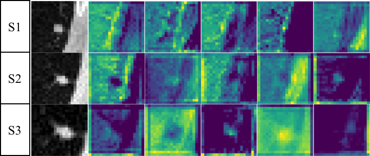
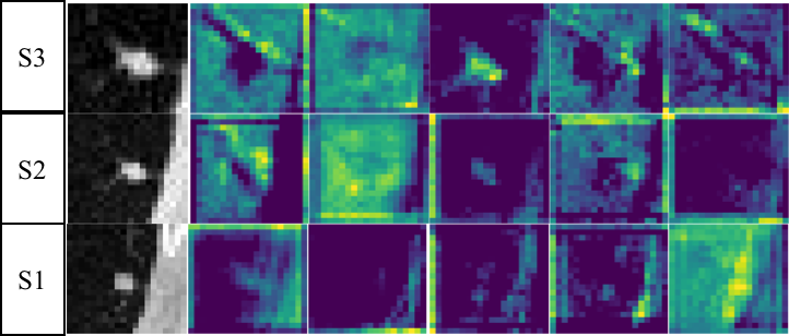
The major advantages of the proposed method can be summarized by two points. First, as shown in Fig. 5, our MGI-CNN could successfully discover morphological and contextual features at different input scales. In Fig. 5(a), we observe that the feature maps in the zoom-in network (i.e., each column in the figure) gradually integrate contextual information in the nodule region. Each sample feature map was extracted from the middle of the sagittal plane in the 3D feature map before concatenation with the next scale input. A similar but reversed pattern in integrating the contextual information can be observed in the zoom-out network (each column in Fig. 5(b)). These different ways of integrating contextual information and extracting features from multi-scale patches could provide complementary information, and thus could enhance performance in the end. Second, our proposed abstract feature integration is useful in terms of information utilization. It is possible to maximize the FP reduction by integrating features at the abstract-level.

With regard to complementary features integration at the abstract-level, we considered three different strategies, i.e., concatenation, element-wise summation, $1\times 1$ convolution [22], commonly used in the literature. The resulting performances are presented in Table 5. Although there is no significant difference among the four methods in average CPM, from a FP reduction perspective, the element-wise summation reported 232 number of FPs, reducing by 31 (vs. concatenation), 103 (vs. skip-connection), and 31 (vs. $1\times 1$ convolution). In this regard, we used element-wise summation in our MGI-CNN.

The 3D patches fed into our network were resized to fit the input receptive field size, i.e., $20\times 20\times 6$. Such image resizing may cause information loss or corruption in the original-sized patches. However, as we can see in Fig. 5, the 3D patches of size $20\times 20\times 6$, in which the nodule still occupies most of the patch, was not affected by the resizing operation. This means that even if the surrounding region information is lost by resizing, the information of the nodule itself could be preserved.

(a) Low confidence
($0.5\leq p<0.7$)

(b) Moderate confidence
($0.7\leq p<0.9$)

(c) High confidence
($0.9\leq p<1$)

Figure 6: Examples of the candidate nodules misclassified to nodule by our MGI-CNN. Based on the output probabilities as nodule, samples are clustered into three groups. The first, second, and third rows correspond to $S1$, $S2$, and $S3$ scale, respectively. The number at the bottom of each column is the output probability as nodule.

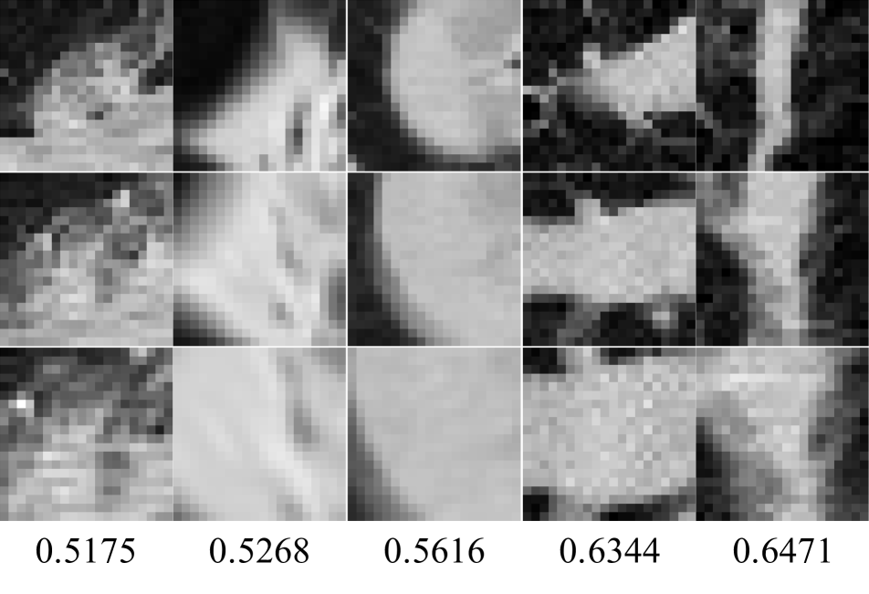
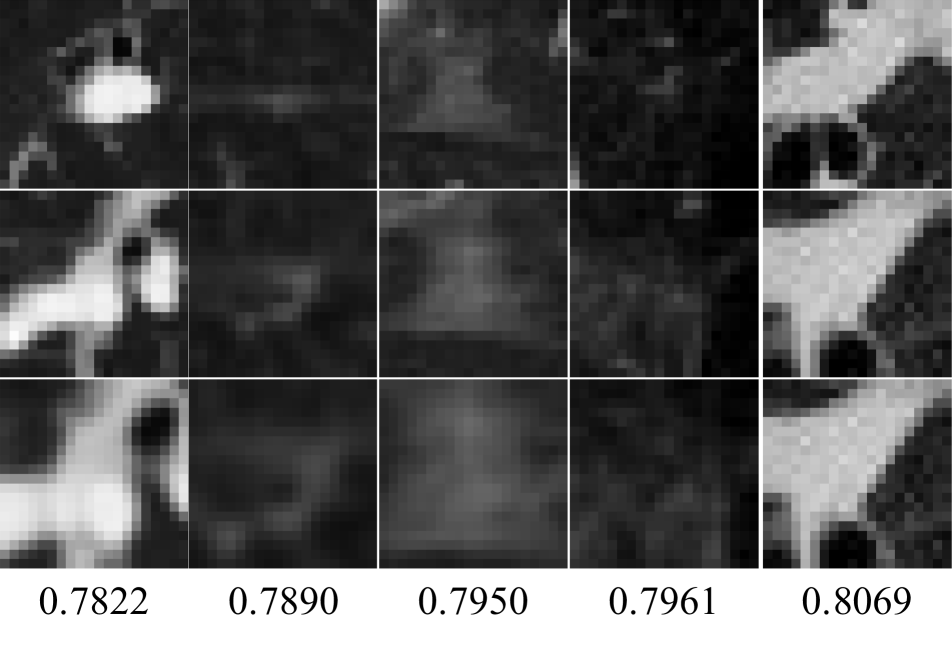
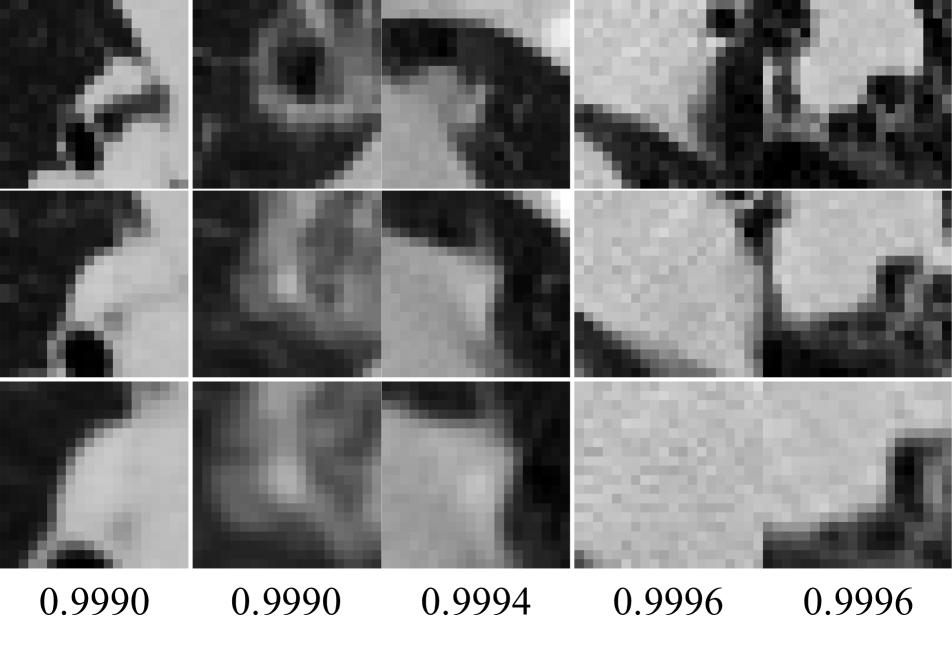
We visually inspected the misclassified candidate nodules. In particular, we first clustered the 232 FPs by our MGI-CNN into three groups based on the their probabilities as nodule: Low Confidence (LC; $0.5\leq p<0.7$), Moderate Confidence (MC; $0.7\leq p<0.9$), and High Confidence (HC; $p>0.9$). The number of FP patches for each group was 33 (LC), 47 (MC), and 152 (HC), respectively. Fig. 6 presents the representative FP 3D patches for three groups. One noticeable thing from the LC and HC groups is that the extracted 3D patches mostly seem to be a subpart of a large tissue or organ, and thus our network failed to find configural patterns necessary to differentiate from non-nodules. For the MC group, patches show relatively low contrasts, which is possibly due to our normalization during preprocessing (Section 4.1). These observations motivate us to extend our network to accommodate an increased number of patches with larger scales and patches normalized in different ways. This would be an interesting direction to further improve the performance.

From a system’s perspective, instead of developing a full pulmonary nodule detection system, which usually consists of a candidate detection part and a FP reduction part, this study mainly focused on improving the FP reduction component. As the proposed approach is independent of candidate screening methods, our network can be combined with any candidate detector. If the proposed network is combined with more high-performance candidate detection methods, we presume to obtain better results.

6 Conclusion

In this paper, we proposed a novel multi-scale gradual integration CNN for FP reduction in pulmonary nodule detection on thoracic CT scans. In our network architecture, we exploited three major strategies: (1) use of multi-scale inputs with different levels of contextual information, (2) gradual integration of the information inherent in different input scales, and (3) multi-stream feature integration by learning in an end-to-end manner. With the first two strategies, we successfully extracted morphological features by gradually integrating contextual information in multi-scale patches. Owing to the third strategy, we could further reduce the number of FPs. In our experiments on the LUNA16 challenge datasets, our network achieved the highest performance with an average CPM of 0.908 on the V1 dataset and an average CPM of 0.942 on the V2 dataset, outperforming state-of-the-art methods by a large margin. In particular, our method obtained promising performances in low FP/scan conditions.

Our current work mostly focused on FP reduction given coordinates of many candidate nodules. We believe that our network can be converted to accomplish positive nodule detection on the low-dose CT scans directly with minor modifications, such as replacing the fully-connected layers with $1\times 1$ convolution layers. For clinical practice, it is also important to classify nodules into various subtypes of solid, non-solid, part-solid, perifissural, calcified, spiculated [3], for which different treatments can be used. Thus, it will be our forthcoming research direction.

References

- [1] S. G. Armato, G. McLennan, L. Bidaut, M. F. McNitt-Gray, C. R. Meyer, A. P. Reeves, B. Zhao, D. R. Aberle, C. I. Henschke, E. A. Hoffman, et al. The Lung Image Database Consortium (LIDC) and Image Database Resource Initiative (IDRI): a Completed Reference Database of Lung Nodules on CT Scans. Medical Physics, 38(2):915–931, 2011.
- [2] P. Cao, X. Liu, J. Yang, D. Zhao, W. Li, M. Huang, and O. Zaiane. A multi-kernel based framework for heterogeneous feature selection and over-sampling for computer-aided detection of pulmonary nodules. Pattern Recognition, 64:327–346, 2017.
- [3] F. Ciompi, K. Chung, S. J. van Riel, A. A. A. Setio, P. K. Gerke, C. Jacobs, E. Th. Scholten, C. Schaefer-Prokop, M. M. W. Wille, A. Marchianò, U. Pastorino, M. Prokop, and B. van Ginneken. Towards Automatic Pulmonary Nodule Management in Lung Cancer Screening with Deep Learning. Scientific Reports, 7(46479), 2017.
- [4] F. Ciompi, B. de Hoop, S. J. van Riel, K. Chung, E. T. Scholten, M. Oudkerk, P. A. de Jong, M. Prokop, and B. van Ginneken. Automatic Classification of Pulmonary Peri-fissural Nodules in Computed Tomography using an Ensemble of 2D Views and a Convolutional Neural Network Out-of-The-Box. Medical Image Analysis, 26(1):195–202, 2015.
- [5] J. Ding, A. Li, Z. Hu, and L. Wang. Accurate Pulmonary Nodule Detection in Computed Tomography Images Using Deep Convolutional Neural Networks. arXiv preprint arXiv:1706.04303, pages 1–9, 2017.
- [6] Q. Dou, H. Chen, L. Yu, J. Qin, and P. A. Heng. Multi-level Contextual 3D CNNs for False Positive Reduction in Pulmonary Nodule Detection. IEEE Transactions on Biomedical Engineering, 64(7):1558–1567, 2017.
- [7] Q. Dou, H. Chen, L. Yu, L. Zhao, J. Qin, D. Wang, V. C. Mok, L. Shi, and P. A. Heng. Automatic Detection of Cerebral Microbleeds From MR Images via 3D Convolutional Neural Networks. IEEE Transactions on Medical Imaging, 35(5):1182–1195, 2016.
- [8] B. Efron and R. Tibshirani. An Introduction to the Bootstrap. Chapman & Hall, 1994.
- [9] A. Esteva, B. Kuprel, R. A. Novoa, J. Ko, S. M. Swetter, H. M. Blau, and S. Thrun. Dermatologist-Level Classification of Skin Cancer with Deep Neural Networks. Nature, 542(7639):115–118, 2017.
- [10] J. Friedman, T. Hastie, R. Tibshirani, and Y. Stanford. Additive Logistic Regression: a Statistical View of Boosting. The Annals of Statistics, 28(2):337–407, 1998.
- [11] X. Glorot and Y. Bengio. Understanding The Difficulty of Training Deep Feedforward Neural Networks. In In Proceedings of the International Conference on Artificial Intelligence and Statistics, pages 249–256, 2010.
- [12] M. K. Gould, J. Fletcher, M. D. Iannettoni, W. R. Lynch, D. E. Midthun, D. P. Naidich, and D. E. Ost. Evaluation of Patients with Pulmonary Nodules: When is it Lung Cancer? ACCP Evidence-Based Clinical Practice Guidelines (2nd edition). Chest, 132(3):108S–130S, 2007.
- [13] M. Havaei, A. Davy, D. Warde-Farley, A. Biard, A. Courville, Y. Bengio, C. Pal, P. M. Jodoin, and H. Larochelle. Brain Tumor Segmentation with Deep Neural Networks. Medical Image Analysis, 35:18–31, 2017.
- [14] S. Honari, J. Yosinski, P. Vincent, and C. Pal. Recombinator Networks: Learning Coarse-to-Fine Feature Aggregation. In Proceedings of the IEEE Conference on Computer Vision and Pattern Recognition, pages 1–11, 2016.
- [15] G. Hounsfield. Computed Medical Imaging. Science, 210(4465), 1980.
- [16] Z. Hu, J. Tang, Z. Wang, K. Zhang, L. Zhang, and Q. Sun. Deep learning for image-based cancer detection and diagnosis - a survey. Pattern Recognition, 83:134–149, 2018.
- [17] C. Jacobs, E. M. van Rikxoort, T. Twellmann, E. T. Scholten, P. A. de Jong, J.-M. Kuhnigk, M. Oudkerk, H. J. de Koning, M. Prokop, C. Schaefer-Prokop, et al. Automatic Detection of Subsolid Pulmonary Nodules in Thoracic Computed Tomography Images. Medical Image Analysis, 18(2):374–384, 2014.
- [18] K. Kamnitsas, C. Ledig, V. F. Newcombe, J. P. Simpson, A. D. Kane, D. K. Menon, D. Rueckert, and B. Glocker. Efficient multi-scale 3D CNN with fully connected CRF for accurate brain lesion segmentation. Medical Image Analysis, 36:61–78, 2017.
- [19] A. Karpathy, G. Toderici, S. Shetty, T. Leung, R. Sukthankar, and L. Fei-Fei. Large-Scale Video Classification with Convolutional Neural Networks. In Proceedings of the IEEE Conference on Computer Vision and Pattern Recognition, pages 1725–1732, 2014.
- [20] Y. Lee, T. Hara, H. Fujita, S. Itoh, and T. Ishigaki. Automated Detection of Pulmonary Nodules in Helical CT Images Based on an Improved Template-Matching Technique. IEEE Transactions on Medical Imaging, 20(7):595–604, 2001.
- [21] Q. Li, S. Sone, and K. Doi. Selective Enhancement Filters for Nodules, Vessels, and Airway Walls in Two- and Three-Dimensional CT Scans. Medical Physics, 30(8):2040–2051, 2003.
- [22] M. Lin, Q. Chen, and S. Yan. Network in Network. arXiv preprint arXiv:1312.4400, 2013.
- [23] T.-Y. Lin, P. Dollár, R. Girshick, K. He, B. Hariharan, and S. Belongie. Feature Pyramid Networks for Object Detection. arXiv preprint arXiv:1612.03144, 2016.
- [24] X. Liu, F. Hou, H. Qin, and A. Hao. Multi-view multi-scale cnns for lung nodule type classification from ct images. Pattern Recognition, 77:262–275, 2018.
- [25] K. Murphy, B. van Ginneken, A. M. Schilham, B. De Hoop, H. Gietema, and M. Prokop. A Large-Scale Evaluation of Automatic Pulmonary Nodule Detection in Chest CT using Local Image Fatures and k-Nearest-Neighbour Classification. Medical Image Analysis, 13(5):757–770, 2009.
- [26] V. Nair and G. E. Hinton. Rectified Linear Units Improve Restricted Boltzmann Machines. In Proceedings of International Conference on Machine Learning, pages 807–814, 2010.
- [27] National Lung Screening Trial Research Team, D. R. Aberle, A. M. Adams, C. D. Berg, W. C. Black, J. D. Clapp, R. M. Fagerstrom, I. F. Gareen, C. Gatsonis, P. M. Marcus, and J. D. Sicks. Reduced Lung-Cancer Mortality with Low-Dose Computed Tomographic Screening. New England Journal of Medicine, 365(5):395–409, 8 2011.
- [28] M. Niemeijer, M. Loog, M. D. Abramoff, M. A. Viergever, M. Prokop, and B. van Ginneken. On Combining Computer-Aided Detection Systems. IEEE Transactions on Medical Imaging, 30(2):215–223, 2011.
- [29] T. Okumura, T. Miwa, J.-I. Kako, S. Yamamoto, R. Matsumoto, Y. Tateno, T. Iinuma, and T. Matsumoto. Automatic Detection of Lung Cancers in Chest CT Images by Variable N-Quoit Filter. In Proceedings of International Conference on Pattern Recognition, volume 2, pages 1671–1673, 1998.
- [30] A. S. Razavian, H. Azizpour, J. Sullivan, and S. Carlsson. CNN Features Off-the-Shelf: An Astounding Baseline for Recognition. In Proceedings of the IEEE Conference on Computer Vision and Pattern Recognition Workshops, pages 512–519, 2014.
- [31] H. R. Roth, L. Lu, J. Liu, J. Yao, A. Seff, K. Cherry, L. Kim, and R. M. Summers. Improving Computer-Aided Detection using Convolutional Neural Networks and Random View Aggregation. IEEE Transactions on Medical Imaging, 35(5):1170–1181, 2016.
- [32] M. Sakamoto, H. Nakano, K. Zhao, and T. Sekiyama. Multi-stage Neural Networks with Single-Sided Classifiers for False Positive Reduction and Its Evaluation Using Lung X-Ray (CT) Images. In Proceedings of International Conference Image Analysis and Processing, pages 370–379, 2017.
- [33] A. A. A. Setio, F. Ciompi, G. Litjens, P. Gerke, C. Jacobs, S. J. Van Riel, M. M. Winkler Wille, M. Naqibullah, C. I. Sánchez, and B. Van Ginneken. Pulmonary Nodule Detection in CT Images: False Positive Reduction Using Multi-View Convolutional Networks. IEEE Transactions on Medical Imaging, 35(5):1160–1169, 2016.
- [34] A. A. A. Setio, C. Jacobs, J. Gelderblom, and B. van Ginneken. Automatic Detection of Large Pulmonary Solid Nodules in Thoracic CT Images. Medical Physics, 42(10):5642–5653, 2015.
- [35] A. A. A. Setio, A. Traverso, T. De Bel, M. S. Berens, C. van den Bogaard, P. Cerello, H. Chen, Q. Dou, M. E. Fantacci, B. Geurts, et al. Validation, Comparison, and Combination of Algorithms for Automatic Detection of Pulmonary Nodules in Computed Tomography Images: The LUNA16 Challenge. Medical Image Analysis, 42:1–13, 2017.
- [36] D. Shen, G. Wu, and H.-I. Suk. Deep Learning in Medical Image Analysis. Annual Review of Biomedical Engineering, 19:221–248, 2017.
- [37] W. Shen, M. Zhou, F. Yang, C. Yang, and J. Tian. Multi-scale Convolutional Neural Networks for Lung Nodule Classification. In Proceedings of International Conference on Information Processing in Medical Imaging, pages 588–599. Springer, 2015.
- [38] W. Shen, M. Zhou, F. Yang, D. Yu, D. Dong, C. Yang, Y. Zang, and J. Tian. Multi-crop convolutional neural networks for lung nodule malignancy suspiciousness classification. Pattern Recognition, 61:663–673, 2017.
- [39] W. Shen, M. Zhou, F. Yang, D. Yu, D. Dong, C. Yang, Y. Zang, and J. Tian. Multi-crop Convolutional Neural Networks for Lung Nodule Malignancy Suspiciousness Classification. Pattern Recognition, 61:663–673, 2017.
- [40] H. C. Shin, H. R. Roth, M. Gao, L. Lu, Z. Xu, I. Nogues, J. Yao, D. Mollura, and R. M. Summers. Deep Convolutional Neural Networks for Computer-Aided Detection: CNN Architectures, Dataset Characteristics and Transfer Learning. IEEE Transactions on Medical Imaging, 35(5):1285–1298, 2016.
- [41] R. L. Siegel, K. D. Miller, and A. Jemal. Cancer Statistics, 2017. CA: A Cancer Journal for Clinicians, 67(1):7–30, 1 2017.
- [42] K. Suzuki, S. G. Armato, F. Li, S. Sone, and K. Doi. Massive Training Artificial Neural Network (MTANN) for Reduction of False Positives in Computerized Detection of Lung Nodules in Low-Dose Computed Tomography. Medical Physics, 30(7):1602–1617, 2003.
- [43] M. Tan, R. Deklerck, B. Jansen, M. Bister, and J. Cornelis. A Novel Computer-Aided Lung Nodule Detection System for CT Images. Medical Physics, 38(10):5630–5645, 2011.
- [44] A. Traverso, E. L. Torres, M. E. Fantacci, and P. Cerello. Computer-Aided Detection Systems to Improve Lung Cancer Early Diagnosis: State-of-the-art and Challenges. In Proceedings of Journal of Physics: Conference Series, volume 841, page 012013, 2017.
- [45] Q. Yang and S. J. Pan. A Survey on Transfer Learning. IEEE Transactions on Knowledge and Data Engineering, 22:1345–1359, 2009.
- [46] X. Ye, X. Lin, J. Dehmeshki, G. Slabaugh, and G. Beddoe. Shape-Based Computer-Aided Detection of Lung Nodules in Thoracic CT Images. IEEE Transactions on Biomedical Engineering, 56(7):1810–1820, 2009.
- [47] J. Zhang, P. M. Atkinson, and M. F. Goodchild. Scale in Spatial Information and Analysis. CRC Press, Taylor and Francis, 2014.