Internal observability of the wave equation in a triangular domain

Abstract.

We investigate the internal observability of the wave equation with Dirichlet boundary conditions in a triangular domain. More precisely, the domain taken into exam is the half of the equilateral triangle. Our approach is based on Fourier analysis and on tessellation theory: by means of a suitable tiling of the rectangle, we extend earlier observability results in the rectangle to the case of a triangular domain. The paper includes a general result relating problems in general domains to their tiles, and a discussion of the triangular case. As an application, we provide an estimation of the observation time when the observed domain is composed by three strips with a common side to the edges of the triangle.

1. Introduction

We consider the problem

(1.1) $$\begin{cases}u_{tt}-\Delta u=0&\text{in }\mathbb{R}\times\Omega\\ u=0&\text{on }\mathbb{R}\times\partial\Omega\\ u(t,0)=u_{0},~{}u_{t}(t,0)=u_{1}&\text{in }\Omega\end{cases}$$

where $\Omega$ is a bounded open domain of $\mathbb{R}^{2}$ that can be tiled by the open triangle $\mathcal{T}$ whose vertices are $(0,0),(1/\sqrt{3},0)$ and $(0,1)$. More precisely, we use the symbol $cl(\Omega)$ to denote the closure of a set $\Omega$ and we say that an open set $\Omega_{1}$ tiles $\Omega_{2}$ if there exist a finite number $N$ of rigid transformations $K_{1},\dots,K_{N}$ such that

$$cl(\Omega_{2})=\bigcup_{h=1}^{N}K_{h}cl(\Omega_{2}).$$

and such that $K_{h}(\Omega_{1})\cap K_{j}(\Omega_{1})=\emptyset$ for all $h\not=j$. The triangle $\mathcal{T}$ is the half of an equilateral triangle of side $2/\sqrt{3}$, and it tiles the rectangle

$$\mathcal{R}:=(0,\sqrt{3})\times(0,1).$$

In particular, we have that the rectangle $\mathcal{R}$ can be tiled by $\mathcal{T}$ by means of $6$ rigid transformations $K_{1},\dots,K_{6}$: to keep the discussion at an introductory level, we postpone the explicit definition of the $K_{h}$’s to Section 3, however such tiling is depicted in Figure 1.

Figure 1. The tiling of $\mathcal{R}$ with $\mathcal{T}$. Note that $K_{1}$ is the identity map, hence $K_{1}(\mathcal{T})=\mathcal{T}$.

As it is well known, a complete orthonormal base for $L^{2}(\mathcal{R})$ is given by the eigenfunctions of $-\Delta$ in $H_{0}^{1}(\mathcal{R})$

$$\overline{e}_{k}:=\sin(\pi k_{1}x_{1}/\sqrt{3})\sin(\pi k_{2}x_{2}),\quad\text{where }k=(k_{1},k_{2}),~{}k_{1},k_{2}\in\mathbb{N}$$

and the associated eigenvalues are $\gamma_{k}=\frac{k_{1}^{2}}{3}+k_{2}^{2}$. In [29], a folding technique (that we recall in detail in Section 3) is used to derive from $\{\overline{e}_{k}\}$ an orthogonal base $\{e_{k}\}$ of $L^{2}(\mathcal{T})$ formed by the eigenfunctions of $-\Delta$ in $H_{0}^{1}(\mathcal{T})$. In particular, $\{e_{k}\}\subset span\{\overline{e}_{k}\}$ and $\{e_{k}\}$ and $\{\overline{e}_{k}\}$ share the same eigenvalues $\gamma_{k}$.

The explicit knowledge of a eigenspace for $H_{0}^{1}(\mathcal{T})$ allows us to set the problem (1.1) (with $\Omega=\mathcal{T}$) in the framework of Fourier analysis. Our goal is to exploit the deep relation between the eigenfunctions for $H_{0}^{1}(\mathcal{R})$ and those of $H_{0}^{1}(\mathcal{T})$ in order to extend known observability results for $\mathcal{R}$ to $\mathcal{T}$.

In particular, we are interested in the internal observability of (1.1), i.e., in the validity of the estimates

$$\|u_{0}\|_{L^{2}(\Omega)}^{2}+\|u_{1}\|^{2}_{H^{-1}(\Omega)}\asymp\int_{0}^{T}\int_{\Omega_{0}}|u(t,x)|^{2}dx$$

where $\Omega_{0}$ is a subset of $\Omega$ and $T$ is sufficiently large. Here and in the sequel $A\asymp B$ means $c_{1}A\leq B\leq c_{2}A$ with some constants $c_{1}$ and $c_{2}$ which are independent from $A$ and $B$. When we need to stress the dependence of these estimates on the couple of constants $c=(c_{1},c_{2})$, we write $A\asymp_{c}B$. Also by writing $A\leq_{c}B$ we mean the inequality $cA\leq B$ while the expression $A\geq_{c}B$ denotes $cA\geq B$.

1.1. Statement of the main results

We begin by introducing a few notations. Let $\{e_{k}\}\subset H^{1}_{0}(\Omega)\cap L^{2}(\Omega)$ be an orthonormal base of $L^{2}(\Omega)$ formed by eigenvalues of $-\Delta$ and let $\{\gamma_{k}\}$ be the associated eigenvalues. Denote by $D^{s}(\Omega)$ the completion of $\{e_{k}\}$ with respect to the Euclidean norm

$$\left\|\sum_{k\in\mathbb{Z}^{2}}c_{k}\gamma_{k}\right\|_{s}:=\left(\sum_{k\in\mathbb{Z}^{2}}\gamma_{k}^{s}|c_{k}|^{2}\right)^{1/2}.$$

Identifying $L^{2}(\Omega)$ with its dual we have

$$D^{0}(\Omega)=L^{2}(\Omega),\quad D^{-1}(\Omega)=H^{-1}(\Omega).$$

We have

Theorem 1.1.

Let $\overline{u}$ be the solution of

(1.2) $$\begin{cases}\overline{u}_{tt}-\Delta\overline{u}=0&\text{on }\mathbb{R}\times{\mathcal{R}}\\ \overline{u}=0&\text{in }\mathbb{R}\times\partial\mathcal{R}\\ \overline{u}(t,0)=\overline{u}_{0},~{}u_{t}(t,0)=\overline{u}_{1}&\text{in }{\mathcal{R}},\end{cases}$$

let $\overline{S}$ be a subset of $\mathcal{R}$ and assume that there exists a constant $T_{\overline{S}}\geq 0$ such that if $T>T_{\overline{S}}$ then there exists a couple of constants $c=(c_{1},c_{2})$ such that $\overline{u}$ satisfies

(1.3) $$\|\overline{u}_{0}\|_{0}^{2}+\|\overline{u}_{1}\|^{2}_{-1}\asymp_{c}\int_{0}^{T}\int_{\overline{S}}|\overline{u}(t,x)|^{2}dx$$

for all $(\overline{u}_{0},\overline{u}_{1})\in D^{0}(\mathcal{R})\times D^{-1}(\mathcal{R})$. Moreover let $u$ be the solution $u$ of

(1.4) $$\begin{cases}u_{tt}-\Delta u=0&\text{on }\mathbb{R}\times{\mathcal{T}}\\ u=0&\text{in }\mathbb{R}\times\partial\mathcal{T}\\ u(t,0)=u_{0},~{}u_{t}(t,0)=u_{1}&\text{in }{\mathcal{T}}.\end{cases}$$

and set

$$S:=\bigcup_{h=1}^{6}(K^{-1}_{h}\overline{S}\cap\mathcal{T})$$

Then for each $T>T_{\overline{S}}$ the solution $u$ satisfies

(1.5) $$\|u_{0}\|_{0}^{2}+\|u_{1}\|^{2}_{-1}\asymp_{c}\int_{0}^{T}\int_{S}|u(t,x)|^{2}dx.$$

for all $(u_{0},u_{1})\in D^{0}(\mathcal{T})\times D^{-1}(\mathcal{T})$.

The result also holds by replacing every occurrence of $\asymp_{c}$ with $\leq_{c}$ or $\geq_{c}$.

We point out that the time of observability $T_{\bar{S}}$ stated in Theorem 1.1, as well as the couple $c$ of constants in the estimates (1.3) and (1.5), are the same for both the domains $\mathcal{R}$ and $\mathcal{T}$. Also note that in Section 3 we prove a slightly stronger version of Theorem 1.1, that is Theorem 3.5: its precise statement requires some technicalities that we chose to avoid here, however we may anticipate to the reader that the assumption on initial data $(\overline{u}_{0},\overline{u}_{1})\in D^{0}(\mathcal{R})\times D^{-1}(\mathcal{R})$ can be weakened by replacing $D^{0}(\mathcal{R})\times D^{-1}(\mathcal{R})$ with an appropriate subspace.

Now we state the second main result of the present paper: its proof strongly relies on Theorem 1.1 and on a couple of technical lemmas that can be found in Section 4.

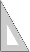
Figure 2. The triangle $\mathcal{T}$ and, in gray, the observation domain $S_{\alpha}$ with $\alpha=0.125$.

Theorem 1.2 (Observability on strips along the edges of $\mathcal{T}$).

Let $\alpha\in(0,1/(3+\sqrt{3})]$. Set $r_{\alpha}:=1-\alpha(3+\sqrt{3}),$

$$S_{\alpha}:={\mathcal{T}}\setminus cl(r_{\alpha}\mathcal{T}+(\alpha,\alpha)),$$

$$t_{\alpha}:=\inf_{k\in\mathbb{N}}\int_{0}^{\alpha}\sin^{2}(\pi kx/\sqrt{3})dx$$

and

$$T_{\alpha}:=8\sqrt{\frac{5}{\sqrt{3}}t_{\alpha}}.$$

If $u$ is the solution of (1.4), then for every $T>T_{\alpha}$

(1.6) $$\|u_{0}\|_{0}^{2}+\|u_{1}\|^{2}_{-1}\leq_{c_{\alpha}}\int_{0}^{T}\int_{S_{\alpha}}|u(t,x)|^{2}dx.$$

for all $(u_{0},u_{1})\in D^{0}(\mathcal{T})\times D^{-1}(\mathcal{T})$ with

$$c_{\alpha}:=\frac{T}{\pi}\left(\frac{t_{\alpha}}{\sqrt{3}}-\frac{40}{3T^{2}}\right)>0.$$

Remark 1.3.

If $\alpha\leq 1/(3+\sqrt{3})\simeq 0.211$ then $S_{\alpha}$ can be equivalently viewed as the intersection between $\mathcal{T}$ and the union of three open strips $s_{1}(\alpha)$, $s_{2}(\alpha)$ and $s_{3}(\alpha)$ of width equal to $\alpha$, each of which has a common side with an edge of $\mathcal{T}$, see Figure 2. If $\alpha=1/(3+\sqrt{3})$ then we are setting as domain of observation $\mathcal{T}\setminus\{(\alpha,\alpha)\}$: note that in this case the point $(\alpha,\alpha)$ is the incenter of $\mathcal{T}$. Finally if $\alpha\geq 1/(3+\sqrt{3})$ then the union of $s_{1}(\alpha),s_{2}(\alpha)$ and $s_{3}(\alpha)$ covers $\mathcal{T}$.

Proof.

Let

$$\bar{S}_{\alpha}:=[(0,\alpha)\times(0,1)]\cup[(0,\sqrt{3})\times(0,\alpha)].$$

Using a result in [18], we show in Lemma 4.2 that if $T>T_{\alpha}$ then the solution $\overline{u}$ of (1.2) satisfies (1.3) for all initial data $(\overline{u}_{0},\overline{u}_{1})\in D^{0}(\mathcal{R})\times D^{-1}(\mathcal{R})$. Then, by Theorem 1.1, setting

$$S^{\prime}_{\alpha}:=\bigcup_{h=1}^{6}(K^{-1}_{h}\overline{S}_{\alpha}\cap\mathcal{T})$$

we have that if $u$ is the solution of (1.4) then $T>T_{\alpha}$ implies

$$\|u_{0}\|_{0}^{2}+\|u_{1}\|^{2}_{-1}\leq c_{\alpha}\int_{0}^{T}\int_{S^{\prime}_{\alpha}}|u(t,x)|^{2}dx.$$

for all $(u_{0},u_{1})\in D^{0}(\mathcal{T})\times D^{-1}(\mathcal{T})$. The claim hence follows by showing that $S_{\alpha}=S^{\prime}_{\alpha}$ for all $\alpha\geq 0$, which is proved in Lemma 4.3. ∎

1.2. Organization of the paper.

In Section 2 we consider a generic domain $\Omega_{1}$ tiling a larger domain $\Omega_{2}$: we establish a result, Theorem 2.7, relating the observability properties of wave equation on $\Omega_{2}$ and on its tile $\Omega_{1}$. In Section 3 we specialize this result to the case in which $\Omega_{1}$ is the triangle $\mathcal{T}$ and the tiled domain $\Omega_{2}$ is the rectangle $\mathcal{R}$: this is the core of the proof of Theorem 1.1. Finally Section 4 is devoted to the proof of Theorem 1.2.

2. An observability result on tilings

The goal of this section is to state an equivalence between an observability problem on a domain $\Omega_{1}$ and an observability problem on a larger domain $\Omega_{2}$, under the assumption that $\Omega_{1}$ tiles $\Omega_{2}$. We begin with some definitions.

Definition 2.1 (Tilings, foldings and prolongations).

Let $\Omega_{1}$ and $\Omega_{2}$ be two open bounded subsets of $\mathbb{R}^{2}$. We say that $\Omega_{1}$ tiles $\Omega_{2}$ if there exists a set $\{K_{h}\}_{h=1}^{N}$ rigid transformations of $\mathbb{R}^{2}$ such that

$$cl(\Omega_{2})=\bigcup_{h=1}^{N}K_{h}cl(\Omega_{1}).$$

and such that $K_{h}(\Omega_{1})\cap K_{j}(\Omega_{1})=\emptyset$ for all $h\not=j$.

Let $(\Omega_{1},\{K_{h}\}_{h=1}^{N})$ be a tiling of $\Omega_{2}$ and $\delta=(\delta_{1},\dots,\delta_{N})\in\{-1,1\}^{N}$. The prolongation with coefficients $\delta$ of a function $u:\Omega_{1}\to\mathbb{R}$ to $\Omega_{2}$ is the function $\mathcal{P}_{\delta}u:\Omega_{2}\to\mathbb{R}$

$$\mathcal{P}_{\delta}u(K_{h}x)=\delta_{h}u(x)\text{ for each }h=1,\dots,N.$$

The folding with coefficients $\delta$ of a function $\overline{u}:\Omega_{2}\to\mathbb{R}$ is the function $\mathcal{F}_{\delta}\overline{u}:\Omega_{1}\to\mathbb{R}$

$$\mathcal{F}_{\delta}\overline{u}(x)=\frac{1}{N^{2}}\sum_{h=1}^{N}\delta_{h}\overline{u}(K_{h}x)\text{ for each }h=1,\dots,N.$$

A tiling $(\Omega_{1},K_{h})$ of $\Omega_{2}$ is admissible if there exists $\delta\in\{-1,1\}^{N}$ such that

(2.1) $$\mathcal{F}_{\delta}\varphi\in H^{1}_{0}(\Omega_{1})\quad\forall\varphi\in H_{0}^{1}(\Omega_{2}).$$

under scripts and we simply write $\mathcal{P}$ and $\mathcal{F}$.

Example 2.1.

We show in Lemma 3.1 below that the tiling of $\mathcal{R}$ with $\mathcal{T}$ depicted in Figure 1 is admissible, in particular (2.1) holds with $\delta=(1,-1,1,1,-1,1)$.

On the other hand the tiling of $\mathcal{R}^{\prime}:=(0,1/\sqrt{3})\times(0,1)$ given by the transformations $K_{1}^{\prime}:=id$ and

$$K_{2}^{\prime}:(x_{1},x_{2})\mapsto-(x_{1},x_{2})+(1/\sqrt{3},1),$$

see Figure 3, is not admissible. Let indeed $v_{1}:=(1/\sqrt{3},0)$, $v_{2}:=(0,1)$ and $x_{\lambda}:=\lambda v_{1}+(1-\lambda)v_{2}$ with $\lambda\in(0,1)$. Then $x_{\lambda}\in\partial\mathcal{T}$ and

$$K_{2}(x_{\lambda})=x_{1-\lambda}$$

Therefore it suffices to choose $\varphi\in H_{0}^{1}(\mathcal{R})$ such that $\varphi(x_{\lambda})\not=\pm\varphi(x_{1-\lambda})$ to obtain

$$\mathcal{F}_{\delta}\varphi(x_{\lambda})=\delta_{1}\varphi(x_{\lambda})+\delta_{2}\varphi(x_{1-\lambda})\not=0$$

for all $\delta_{1},\delta_{2}\in\{-1,1\}$. Consequently $\mathcal{F}_{\delta}\varphi\not\in H_{0}^{1}(\mathcal{T})$ for all $\delta\in\{-1,1\}^{2}$.

Figure 3. A non-admissible tiling of $\mathcal{R}^{\prime}=(0,1/\sqrt{3})\times(0,1)$ with $\mathcal{T}$.

Remark 2.2.

We borrowed the notion of prolongation and folding from [29]: while our definition of $\mathcal{P}_{\delta}$ is exactly as it is given in [29], we introduced a normalizing term $1/N^{2}$ in the definition of $\mathcal{F}_{\delta}$ in order to enlighten the notations. Note that the following equality holds:

(2.2) $$\mathcal{F}_{\delta}(\mathcal{P}_{\delta}u)=\frac{1}{N}u$$

for all $u:\Omega_{1}\to\mathbb{R}$.

Also remark that we shall need to prolong and fold also functions $u:\mathbb{R}\times\Omega_{1}\to\mathbb{R}$ and $\bar{u}:\mathbb{R}\times\Omega_{2}\to\mathbb{R}$, in this case the definition of $\mathcal{P}$ and $\mathcal{F}$ naturally extends by applying the transformations $K_{h}$’s to the spatial variables $x$. For instance if $u:\mathbb{R}\times\Omega_{1}\to\mathbb{R}$ then its prolongation to $\mathbb{R}\times\Omega_{2}$ reads

$$\mathcal{P}_{\delta}u(t,K_{h}x)=\delta_{h}u(t,x).$$

We want to establish a relation between solutions of a wave equation with Dirichlet boundary conditions and their prolongation. To this end we introduce the notations

$$\mathcal{P}_{\delta}L^{2}(\Omega_{1}):=\{\mathcal{P}_{\delta}u\mid u\in L^{2}(\Omega_{1})\},$$

$$\mathcal{P}_{\delta}H^{1}_{0}(\Omega_{1}):=\{\mathcal{P}_{\delta}u\mid u\in H^{1}_{0}(\Omega_{1})\}$$

and

$$\mathcal{P}_{\delta}H^{-1}(\Omega_{1}):=\{\mathcal{P}_{\delta}u\mid u\in H^{-1}(\Omega_{1})\}.$$

Note that $\mathcal{P}_{\delta}L^{2}(\Omega_{1})\subset L^{2}(\Omega_{2})$, $\mathcal{P}_{\delta}H^{1}_{0}(\Omega_{1})\subset H^{1}_{0}(\Omega_{2})$ and $\mathcal{P}_{\delta}H^{-1}(\Omega_{1})\subset H^{-1}(\Omega_{1})$ .

All results below hold under the following assumptions on the domains $\Omega_{1}$, $\Omega_{2}$ and on a base $\{e_{k}\}$ for $L^{2}(\Omega_{1})$:

Assumption 1.

$(\Omega_{1},\{K_{h}\}_{h=1}^{N})$ is an admissible tiling of $\Omega_{2}$.

Assumption 2.

$\{e_{k}\}$ is a base of eigenvectors of $-\Delta$ in $H^{1}_{0}(\Omega_{1})$, it is defined on $\Omega_{1}\cup\Omega_{2}$ and there exists $\delta\in\{-1,1\}^{N}$ such that

$$\mathcal{P}_{\delta}(e_{k}|_{\Omega_{1}})=e_{k}|_{\Omega_{2}}$$

for each $k\in\mathbb{N}$.

Remark 2.3 (Some remarks on Assumption 2).

We note that Assumption 2 can be equivalently stated as

(2.3) $$e_{k}(K_{h}x)=\delta_{h}e_{k}(x)\quad\text{ for all $x\in\Omega_{1}$, $h=1,\dots,N$, $k\in\mathbb{N}$.}$$

Indeed, by definition of prolongation and noting $\delta_{h}^{2}\equiv 1$, we have

$$e_{k}(K_{h}x)=\delta_{h}^{2}e_{k}(K_{h}x)=\delta_{h}\mathcal{P}_{\delta}e_{k}(x)=\delta_{h}e_{k}(x).$$

for every $x\in\Omega_{1}$, $h=1,\dots,N$ and $k\in\mathbb{N}$.
Also remark that, in view of (2.2), Assumption 2 also implies

(2.4) $$\mathcal{F}_{\delta}e_{k}=\frac{1}{N}e_{k}.$$

Example 2.4.

Let $\Omega_{1}=(0,\pi)^{2}$ and $\Omega_{2}=(0,2\pi)^{2}$. Consider the transformations of $\mathbb{R}^{2}$

$$\begin{array}[]{ll}K_{1}:=\text{id},&~{}K_{2}:(x_{1},x_{2})\mapsto(-x_{1}+2\pi,x_{2}),\\ K_{3}:(x_{1},x_{2})\mapsto(x_{1},-x_{2}+2\pi),&~{}K_{4}:(x_{1},x_{2})\mapsto-(x_{1},x_{2})+(2\pi,2\pi)\end{array}.$$

Then $\{\Omega_{1},\{K_{h}\}_{h=1}^{4}\}$ is a tiling for $\Omega_{2}$. In particular, Assumption 1 is satisfied: indeed setting $\delta=(1,-1,-1,1)$ we have for each $\varphi\in H_{0}^{1}(\Omega_{2})$

$$\mathcal{F}_{\delta}\varphi(x)=0\quad\forall x\in\partial\Omega_{1}.$$

Also note that the functions

$$e_{k}(x):=\sin(k_{1}x_{1})\sin(k_{2}x_{2})\quad k=(k_{1},k_{2})\in\mathbb{N}^{2}$$

satisfy Assumption 2, indeed they are a base for $L^{2}(\Omega_{1})$ composed by eigenfunctions of $-\Delta$ in $H_{0}^{1}(\Omega_{1})$ and

$$e_{k}(K_{h}x):=\delta_{h}e_{k}(x)$$

for all $x\in\mathbb{R}^{2}$, $h=1,\dots,4$ and $k\in\mathbb{N}^{2}$. The space $\mathcal{P}_{\delta}L^{2}(\Omega_{1})$ in this case coincides with the space of so-called $(2,2)$-cyclic functions, i.e., functions in $L^{2}(\Omega_{2})$ which are odd with respect to both axes $x_{1}=\pi$ and $x_{2}=\pi$. We refer to [17] for some results on observability of wave equation with $(p,q)$-cyclic initial data.

Our starting point is to show that, under Assumptions 1 and 2, the base of eigenfunctions $\{e_{k}\}$ is also a base of eigenfunctions also for an appropriate subspace of $L^{2}(\Omega_{2})$, and to compute the associated coefficients.

Lemma 2.5.

Let $\Omega_{1},\Omega_{2}$ and $\{e_{k}\}$ satisfy Assumption 1 and Assumption 2.

Then $\{e_{k}\}\subset H^{1}_{0}(\Omega_{2})$ and it is also a complete base for $\mathcal{P}_{\delta}L^{2}(\Omega_{1})$ formed by eigenfunctions of $-\Delta$ in $\mathcal{P}_{\delta}H_{0}^{1}(\Omega)$.

In particular, for every $k\in\mathbb{N}$, if $u_{k}$ is the coefficient of $u\in L^{2}(\Omega_{1})$ (with respect to $e_{k}$) then $Nu_{k}$ is the coefficient of $\mathcal{P}_{\delta}u$.

Proof.

The proof is organized two steps.
Claim 1: $\{e_{k}\}$ is a set of eigenfunctions of $-\Delta$ in $H_{0}^{1}(\Omega_{2})$. Extending a result given in [29], we need to show that, under Assumption 1 and Assumption 2, if $e_{k}\in H_{0}^{1}(\Omega_{1})$ is a solution of the boundary value problem

$$\int_{\Omega_{1}}\nabla e_{k}\nabla\varphi dx=\int_{\Omega_{1}}\gamma_{k}e_{k}\varphi dx\quad\forall\varphi\in H_{0}^{1}(\Omega_{1})$$

for some $\gamma_{k}\in\mathbb{R}$, then $e_{k}$ is also solution of the boundary value problem on $\Omega_{2}$

$$\int_{\Omega_{2}}\nabla e_{k}\nabla\varphi dx=\int_{\Omega_{2}}\gamma_{k}e_{k}\varphi dx\quad\forall\varphi\in H_{0}^{1}(\Omega_{2}).$$

Now, recall from Assumption 1 that if $\varphi\in H_{1}^{0}(\Omega_{2})$ then $\mathcal{F}_{\delta}\varphi\in H_{1}^{0}(\Omega_{1})$. Then it follows again from Assumption 1 and from Assumption 2 (in particular by recalling that $K_{h}$’s are isometries and (2.3)) that for all $\varphi\in H_{0}^{1}(\Omega_{2})$

$$\int_{\Omega_{2}}\nabla e_{k}(x) \nabla\varphi(x)dx=\int_{\bigcup_{h=1}^{N}K_{h}\Omega_{1}}\nabla e_{k}(x)\nabla\varphi(x)dx$$

$$=\sum_{h=1}^{N}\int_{\Omega_{1}}\nabla e_{k}(K_{h}x)\nabla\varphi(K_{h}x)dx=\int_{\Omega_{1}}\nabla e_{k}(x)\sum_{h=1}^{N}\delta_{h}\nabla\varphi(K_{h}x)dx$$

$$=\int_{\Omega_{1}}\nabla e_{k}(x)\nabla\mathcal{F}_{\delta}\varphi(x)dx=\int_{\Omega_{1}}\gamma_{k}e_{k}(x)\mathcal{F}_{\delta}\varphi(x)dx$$

$$=\int_{\Omega_{2}}\gamma_{k}e_{k}(x)\varphi(x)dx.$$

and this completes the proof of Claim 1.

Claim 2: completeness of $\{e_{k}\}$ and computation of coefficients By Assumption 1 and Assumption 2 and by recalling $\delta_{h}^{2}=1$ for each $h=1,\dots,N$, we have

$$\int_{\Omega_{2}}\mathcal{P}_{\delta}u(x)e_{k}(x)dx =\int_{\Omega_{2}}\mathcal{P}_{\delta}u(x)\mathcal{P}_{\delta}e_{k}(x)dx$$

$$=\sum_{h=1}^{N}\int_{K_{h}\Omega_{1}}\mathcal{P}_{\delta}u(x)\mathcal{P}e_{k}(x)dx$$

$$=\sum_{h=1}^{N}\int_{K_{h}\Omega_{1}}\delta_{h}^{2}u(K_{h}x)e_{k}(K_{h}x)dx$$

$$=\sum_{h=1}^{N}\int_{\Omega_{1}}u(x)e_{k}(x)dx=N\int_{\Omega_{1}}u(x)e_{k}(x)dx,$$

where the second to last equality holds because $K_{h}$’s are rigid transformations. Then we may deduce two facts: first if $\{u_{k}\}$ are the coefficients of $u\in L^{2}(\Omega_{1})$ then $\{Nu_{k}\}$ are coefficients of $\mathcal{P}_{\delta}u$. Secondly, $\{e_{k}\}$ is a complete base for $\mathcal{P}_{\delta}L^{2}(\Omega_{1})$, indeed if the coefficients of $\mathcal{P}_{\delta}u$ are identically null, then also the coefficients of $u$ are identically null: since $\{e_{k}\}$ is complete for $\Omega_{1}$ then $u\equiv 0$ and, consequently, $\mathcal{P}_{\delta}u\equiv 0$, as well. $\Omega_{2}$ and, consequently, $\partial\Omega_{2}\subset\bigcup_{h=1}^{N}K_{h}(\partial\Omega_{1})$. ∎

Next result establishes a relation between solutions of wave equations on tiles and their prolongations.

Lemma 2.6.

Let $\Omega_{1},\Omega_{2}$ and $\{e_{k}\}$ satisfy Assumption 1 and Assumption 2. Let $u$ be the solution of

(2.5) $$\begin{cases}u_{tt}-\Delta u=0&\text{in }\mathbb{R}\times\Omega_{1}\\ u=0&\text{on }\mathbb{R}\times\partial\Omega_{1}\\ u(t,0)=u_{0},~{}u_{t}(t,0)=u_{1}&\text{in }\Omega_{1}\end{cases}$$

Then $u$ is well defined in $\Omega_{1}\cup\Omega_{2}$ and $\overline{u}=Nu|_{\Omega_{2}}$ is the solution of

(2.6) $$\begin{cases}\overline{u}_{tt}-\Delta\overline{u}=0&\text{on }\mathbb{R}\times\Omega_{2}\\ \overline{u}=0&\text{in }\mathbb{R}\times\partial\Omega_{2}\\ \overline{u}(t,0)=\mathcal{P}_{\delta}u_{0},~{}\overline{u}(t,0)=\mathcal{P}_{\delta}u_{1}&\text{in }\Omega_{2}\end{cases}$$

Conversely, if $\bar{u}$ is the solution of (2.6) then $\mathcal{F}_{\delta}\bar{u}$ is the solution of (2.5) and for every $h=1,\dots,N$

(2.7) $$\mathcal{F}_{\delta}\bar{u}(t,x)=\frac{\delta_{h}}{N}\bar{u}(t,K_{h}x)\quad\text{for each $x\in\Omega_{1}$}.$$

Proof.

Let $\{\gamma_{k}\}$ be the sequence of eigenvalues associated to $\{e_{k}\}$ and set $\omega_{k}=\sqrt{\gamma_{k}}$, for every $k\in\mathbb{N}$. Expanding $u(t,x)$ with respect to $e_{k}$ we obtain

$$u(t,x)=\sum_{k=1}^{\infty}(a_{k}e^{i\omega_{k}t}+b_{k}e^{-i\omega_{k}t})e_{k}(x)$$

with $a_{k}$ and $b_{k}$ depending only the coefficients $c_{k}$ and $d_{k}$ of $u_{0}$ and $u_{1}$ with respect to $\{e_{k}\}$. In particular $a_{k}+b_{k}=c_{k}$ and $a_{k}-b_{k}=-id_{k}/\omega_{k}$. We then have that the natural domain of $u$ coincides with the one of $\{e_{k}\}$’s, hence it is included in $\Omega_{1}\cup\Omega_{2}$. By Lemma 2.5 the coefficients of $\mathcal{P}_{\delta}u_{0}$ and $\mathcal{P}_{\delta}u_{1}$ are $Nc_{k}$ and $Nd_{k}$, respectively. Then it is immediate to verify that

$$Nu(t,x)=\sum_{k=1}^{\infty}(Na_{k}e^{i\omega_{k}t}+Nb_{k}e^{-i\omega_{k}t})e_{k}(x)$$

is the solution of (2.6).

Now, let

$$\bar{u}(t,x)=\sum_{k=1}^{\infty}(\bar{a}_{k}e^{i\omega_{k}t}+\bar{b}_{k}e^{-i\omega_{k}t})e_{k}(x)$$

be the solution of (2.6), and note that, by the reasoning above, setting $a_{k}:=\frac{1}{N}\bar{a}_{k}$ and $b_{k}:=\frac{1}{N}\bar{b}_{k}$ we have that

$$u(t,x):=\sum_{k=1}^{\infty}(a_{k}e^{i\omega_{k}t}+b_{k}e^{-i\omega_{k}t})e_{k}(x)=\frac{1}{N}\bar{u}(t,x)$$

is the solution of (2.5). Hence to prove that $u(t,x)=\mathcal{F}_{\delta}\bar{u}(t,x)$ it it suffices to note that by Assumption 1 (see in particular (2.4))

$$\mathcal{F}_{\delta}\bar{u}(t,x) =\sum_{k=1}^{\infty}(\bar{a}_{k}e^{i\omega_{k}t}+\bar{b}_{k}e^{-i\omega_{k}t})\mathcal{F}_{\delta}e_{k}(x)$$

$$=\frac{1}{N}\sum_{k=1}^{\infty}(\bar{a}_{k}e^{i\omega_{k}t}+\bar{b}_{k}e^{-i\omega_{k}t})e_{k}(x)=\frac{1}{N}\bar{u}(t,x).$$

Finally, we show (2.7): for each $h=1,\dots,N$ we have

$$\bar{u}(t,x) =\delta_{h}^{2}\bar{u}(t,x)=\delta_{h}\sum_{k=1}^{\infty}(\bar{a}_{k}e^{i\omega_{k}t}+\bar{b}_{k}e^{-i\omega_{k}t})\delta_{h}e_{k}(x)$$

$$=\sum_{k=1}^{\infty}(\bar{a}_{k}e^{i\omega_{k}t}+\bar{b}_{k}e^{-i\omega_{k}t})e_{k}(K_{h}x)=\delta_{h}\bar{u}(t,K_{h}x)$$

and this concludes the proof. (2.6). ∎

We are now in position to state the main result of this section, that bridges observability of tiles with their prolongations.

Theorem 2.7.

Let $\Omega_{1},\Omega_{2}$ and $\{e_{k}\}$ satisfy Assumption 1 and Assumption 2. Let $u$ be the solution of

(2.8) $$\begin{cases}u_{tt}-\Delta u=0&\text{on }\mathbb{R}\times\Omega_{1}\\ u=0&\text{in }\mathbb{R}\times\partial\Omega_{1}\\ u(t,0)=u_{0},~{}u_{t}(t,0)=u_{1}&\text{in }\Omega_{1}\end{cases}$$

with $u_{0},u_{1}\in D^{0}(\Omega_{1})\times D^{-1}(\Omega_{1})$ and let $\overline{u}$ be the solution of

(2.9) $$\begin{cases}u_{tt}-\Delta u=0&\text{on }\mathbb{R}\times\Omega_{2}\\ u=0&\text{in }\mathbb{R}\times\partial\Omega_{2}\\ u(t,0)=\mathcal{P}_{\delta}u_{0},~{}u_{t}(t,0)=\mathcal{P}_{\delta}u_{1}&\text{in }\Omega_{2}.\end{cases}$$

Also let $\bar{S}\subset\Omega_{2}$ and define

$$S:=\bigcup_{h=1}^{N}K_{h}^{-1}\overline{S}\cap\Omega_{1}.$$

Then for every $T>0$ and for every couple $c=(c_{1},c_{2})$ of positive constants, the inequalities

(2.10) $$\|u_{0}\|_{0}^{2}+\|u_{1}\|^{2}_{-1}\asymp_{c}\int_{0}^{T}\int_{S}|u(t,x)|^{2}dx.$$

hold if and only if

(2.11) $$\|\mathcal{P}_{\delta}u_{0}\|_{0}^{2}+\|\mathcal{P}_{\delta}u_{1}\|^{2}_{-1}\asymp_{c}\int_{0}^{T}\int_{\overline{S}}|\overline{u}(t,x)|^{2}dx.$$

Proof.

By Lemma 2.6, $u$ and $\overline{u}$ satisfy

$$u(t,x)=\frac{\delta_{h}}{N}\overline{u}(t,K_{h}x)\quad\text{ for all }h=1,\dots,N.$$

Since $\Omega_{1}$ tiles $\Omega_{2}$, then setting $S_{h}:=K_{h}^{-1}\bar{S}\cap\Omega_{1}$ we have $S=\bigcup_{h=1}^{N}S_{h}$ and $\overline{S}=\bigcup_{h=1}^{N}K_{h}S_{h}$, and that these unions are disjoint. Hence, also recalling $|\delta_{h}|\equiv 1$ we have

$$\int_{I}\int_{\overline{S}}|\overline{u}(t,x)|^{2}dx =\sum_{h=1}^{N}\int_{I}\int_{K_{h}S_{h}}|\overline{u}(t,x)|^{2}dx$$

$$=\sum_{h=1}^{N}\int_{I}\int_{S_{h}}|\overline{u}(t,K_{h}x)|^{2}dx$$

$$=N^{2}\sum_{h=1}^{N}\int_{I}\int_{S_{h}}|\frac{\delta_{h}}{N}\overline{u}(t,K_{h}x)|^{2}dx$$

$$=N^{2}\sum_{h=1}^{N}\int_{I}\int_{S_{h}}|u(t,x)|^{2}dx$$

$$=N^{2}\int_{I}\int_{S}|u(t,x)|^{2}dx$$

Finally, by Lemma 2.5

$$\|\mathcal{P}_{\delta}u_{0}\|^{2}_{0}=N^{2}\|u_{0}\|_{0}^{2}\quad\text{and}\quad\|\mathcal{P}_{\delta}u_{1}\|^{2}_{-1}=N^{2}\|u_{1}\|_{-1}^{2}.$$

and this implies the equivalence between (2.10) and (2.11). ∎

3. Proof of Theorem 1.1

The proof of Theorem 1.1 is based on the application of Theorem 2.7 to the particular case

$$\Omega_{1}=\mathcal{T}\quad\text{and}\quad\Omega_{2}=\mathcal{R}.$$

$2/\sqrt{3}$) as well as side $2/\sqrt{3}$. wave equation in $\mathcal{T}$ bridge the well-established solutions in the rectangle $\mathcal{R}$ to the ones with domain equal to the rhombus or the hexagon.

We then need to admissibly tile $\mathcal{R}$ with $\mathcal{T}$ and a base $\{e_{k}\}$ formed by the eigenfunctions of $-\Delta$ in $H_{0}^{1}(\mathcal{T})$ satisfying Assumption 2. Such ingredients are provided in [29]: in order to introduce them we need some notations. We consider the Pauli matrix

$$\sigma_{z}:=\begin{pmatrix}1&0\\ 0&-1\\ \end{pmatrix}$$

and the rotation matrix

$$R_{\alpha}:=\begin{pmatrix}\cos\alpha&\sin\alpha\\ -\sin\alpha&\cos\alpha\\ \end{pmatrix}$$

where $\alpha:=\pi/3$. Now let $v_{1}:=(0,1/\sqrt{3})$ and $v_{2}:=(0,1)$ be two of the three vertices of $\mathcal{T}$ and define the transformations from $\mathbb{R}^{2}$ onto itself

(3.1) $$\small{\begin{array}[]{ll}K_{1}:=id;&\quad K_{4}:x\mapsto-R_{\alpha}(x-v_{2})+3v_{1}\\ K_{2}:x\mapsto-R_{\alpha}\sigma_{z}(x-v_{2})+v_{2};&\quad K_{5}:x\mapsto-R_{\alpha}(x-v_{2})+3v_{1}+v_{2}\\ K_{3}:x\mapsto R_{\alpha}(x-v_{2})+v_{2};&\quad K_{6}:x\mapsto-x+3v_{1}+v_{2}\end{array}}$$

and note $(\mathcal{T},\{K_{h}\}_{h=1}^{6})$ is a tiling for $\mathcal{R}$. Indeed

(3.2) $$cl(\mathcal{R})=\bigcup_{h=1}^{6}K_{h}cl(\mathcal{T}),$$

and the sets $K_{h}\mathcal{T}$, for $h=1,\dots,6$, do not overlap – see Figure 4 and [29].

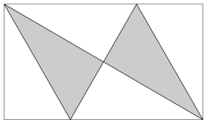
Figure 4. The tiling of $\mathcal{R}$ with $\mathcal{T}$, the gray areas correspond to negative $\delta_{h}$’s.

We set

$$\delta:=(1,-1,1,1,-1,1).$$

and, in next result, we prove that $\mathcal{T}$ admissibly tiles $\mathcal{R}$.

Lemma 3.1.

$(\mathcal{T},\{K_{h}\}_{h=1}^{6})$ is an admissible tiling of $\mathcal{R}$.

Proof.

We want to show that if $\varphi\in H_{0}^{1}(\mathcal{R})$ then $\mathcal{F}_{\delta}\varphi\in H_{0}^{1}(\mathcal{T})$. To this end let $v_{0}:=(0,0)$, $v_{1}:=(1/\sqrt{3},0)$ and $v_{2}:=(0,1)$ be the vertices of $\mathcal{T}$ and define

$$x_{ij}^{\lambda}:=\lambda v_{i}+(1-\lambda)v_{j}.$$

so that $\partial\mathcal{T}=\{x_{ij}^{\lambda}\mid\lambda\in[0,1],0\leq i<j\leq 2\}$. By a direct computation, for all $\lambda\in[0,1]$

$$K_{1}(x_{01}^{\lambda}),K_{6}(x_{01}^{\lambda})\in\partial\mathcal{R},$$

$$K_{2}(x_{01}^{\lambda})=K_{4}(x_{01}^{\lambda}),$$

and

$$K_{3}(x_{02}^{\lambda})=K_{5}(x_{02}^{\lambda}).$$

Since $\varphi\in H_{0}^{1}(\mathcal{R})$ then $\mathcal{F}_{\delta}\varphi(x_{01}^{\lambda})=0$. Similarly, for all $\lambda\in[0,1]$

$$K_{1}(x_{02}^{\lambda}),K_{6}(x_{02}^{\lambda})\in\partial\mathcal{R},$$

$$K_{2}(x_{02}^{\lambda})=K_{3}(x_{02}^{\lambda}),$$

and

$$K_{4}(x_{02}^{\lambda})=K_{5}(x_{02}^{\lambda})$$

therefore $\mathcal{F}_{\delta}\varphi(x_{02}^{\lambda})=0$ for all $\lambda\in[0,1]$. Finally for all $\lambda\in[0,1]$

$$K_{3}(x_{12}^{\lambda}),K_{4}(x_{12}^{\lambda})\in\partial\mathcal{R},$$

$$K_{1}(x_{12}^{\lambda})=K_{2}(x_{12}^{\lambda}),$$

and

$$K_{5}(x_{12}^{\lambda})=K_{6}(x_{12}^{\lambda})$$

therefore we get also in this case $\mathcal{F}_{\delta}\varphi(x_{12}^{\lambda})=0$ for all $\lambda\in[0,1]$ and we may conclude that $\mathcal{F}_{\delta}\varphi\in H_{0}^{1}(\mathcal{T})$. ∎

Remark 3.2.

Lemma 3.1 was remarked in [29, p.312], but to the best of our knowledge, this is the first time an explicit proof is provided.

Now, consider the eigenfunctions of $-\Delta$ in $H_{0}^{1}(\mathcal{R})$:

$$\overline{e}_{k}(x_{1},x_{2}):=\sin(\pi k_{1}\frac{x_{1}}{\sqrt{3}})\sin(\pi k_{2}x_{2}),\quad k=(k_{1},k_{2})\in\mathbb{N}^{2}.$$

We finally define for every $k\in\mathbb{N}^{2}$

(3.3) $$e_{k}(x):=N^{2}\mathcal{F}_{\delta}\overline{e}_{k}=\sum_{h=1}^{6}\delta_{h}\overline{e}_{k}(K_{h}x).$$

Next result, proved in [29], states that Assumption 2 is satisfied by $\{e_{k}\}$.

Lemma 3.3.

The set of functions $\{e_{k}\}$ defined in (3.3) is a complete orthogonal base for $\mathcal{T}$ formed by the eigenfunction of $-\Delta$ in $H_{0}^{1}(\mathcal{T})$. Furthermore $\mathcal{P}_{\delta}e_{k}(x)=e_{k}(x)$.

Remark 3.4.

For each $k\in\mathbb{N}^{2}$, the eigenfunctions $e_{k}$ and $\bar{e}_{k}$ share the same eigenvalue $\gamma_{k}=\pi^{2}(\frac{k_{1}^{2}}{3}+k_{2}^{2})$, see [29].

Next gives access to classical results on observability of rectangular membranes for the study of triangular domains.

Theorem 3.5.

Let $\overline{S}\subset\mathcal{R}$ be such that the solution $\overline{u}$ of

(3.4) $$\begin{cases}u_{tt}-\Delta u=0&\text{on }\mathbb{R}\times\mathcal{R}\\ u=0&\text{in }\mathbb{R}\times\partial\mathcal{R}\\ u(t,0)=\mathcal{P}_{\delta}u_{0},~{}u(t,0)=\mathcal{P}_{\delta}u_{1}&\text{in }\mathcal{R}.\end{cases}$$

satisfies for some $T>0$ and some couple of positive constants $c=(c_{1},c_{2})$

(3.5) $$\|\mathcal{P}_{\delta}u_{0}\|_{0}^{2}+\|\mathcal{P}_{\delta}u_{1}\|^{2}_{-1}\asymp_{c}\int_{0}^{T}\int_{\overline{S}}|\overline{u}(t,x)|^{2}dx$$

for all $(u_{0},u_{1})\in D^{0}(\mathcal{T})\times D^{-1}(\mathcal{T})$. Moreover let

$$S:=\bigcup_{h=1}^{6}(K^{-1}_{h}\overline{S}\cap\mathcal{T})$$

Then the solution $u$ of

(3.6) $$\begin{cases}u_{tt}-\Delta u=0&\text{on }\mathbb{R}\times\mathcal{T}\\ u=0&\text{in }\mathbb{R}\times\partial\mathcal{T}\\ u(t,0)=u_{0},~{}u_{t}(t,0)=u_{1}&\text{in }\mathcal{T}.\end{cases}$$

satisfies

(3.7) $$\|u_{0}\|_{0}^{2}+\|u_{1}\|^{2}_{-1}\asymp_{c}\int_{0}^{T}\int_{S}|u(t,x)|^{2}dx.$$

for all $(u_{0},u_{1})\in D^{0}(\mathcal{T})\times D^{-1}(\mathcal{T})$.

Proof.

Since $\mathcal{T},\mathcal{R}$ and $\{e_{k}\}$ satisfy Assumption 1 and Assumption 2, then the claim follows by a direct application of Theorem 2.7 with $\Omega_{1}=\mathcal{T}$ and $\Omega_{2}=\mathcal{R}$. ∎

We conclude this section by showing that Theorem 1.1 is a direct consequence of Theorem 3.5:

Proof of Theorem 1.1.

By Lemma 2.5, if $(u_{0},u_{1})\in D^{0}(\mathcal{T})\times D^{-1}(\mathcal{T})$ then $(\mathcal{P}_{\delta}u_{0},\mathcal{P}_{\delta}u_{1})\in D^{0}(\mathcal{R})\times D^{-1}(\mathcal{R})$. The claim hence follows by Theorem 3.5. also apply. ∎

4. Proof of Theorem 1.2

In this Section we keep all the notations used in Section 3. So that for instance $\{K_{h}\}$ are the transformations given in (3.1) and $\delta=(1,-1,1,1,-1,1)$. Also recall the definitions

$$S_{\alpha}:={\mathcal{T}}\setminus cl(r_{\alpha}\mathcal{T}+(\alpha,\alpha))$$

and

$$\overline{S}_{\alpha}:=[(0,\sqrt{3})\times(0,\alpha)]\cup[(0,\alpha)\times(0,1)]$$

As mentioned in the Introduction, to prove Theorem 1.2 we need two auxiliary results: Lemma 4.2, which is an internal observability result on rectangles, and Lemma 4.3, which is a geometric result characterizing $S_{\alpha}$.

We begin by recalling the following:

Proposition 4.1 ([18, Proposition 1.1]).

Let $\Omega=(0,\ell_{1})\times(0,\ell_{2})$, let $J_{1}\subset(0,\ell_{1})$ and $J_{2}\subset(0,\ell_{2})$ and define

$$\overline{S}:=[J_{1}\times(0,\ell_{2})]\cup[(0,\ell_{1})\times J_{2}]$$

Also define the positive constants

$$t_{1}:=\inf_{k\in\mathbb{N}}\int_{J_{1}}\sin\left(\frac{\pi kx}{\ell_{1}}\right)dx,\quad t_{2}:=\inf_{k\in\mathbb{N}}\int_{J_{2}}\sin\left(\frac{\pi kx}{\ell_{2}}\right)dx.$$

and

$$m:=\min\left\{\frac{t_{1}}{\ell_{1}},\frac{t_{2}}{\ell_{2}}\right\}$$

If $T>0$ satisfies the condition

(4.1) $$\frac{(\ell_{1}^{2}+\ell_{2}^{2})(\ell_{1}^{4}+\ell_{2}^{4})}{T^{2}\ell_{1}^{2}\ell_{2}^{2}}<m$$

then the solutions $u$ of (1.1) satisfy the estimate

(4.2) $$|u_{0}|_{0}^{2}+|u_{1}|^{2}_{-1}\leq_{c}\int_{0}^{T}\int_{\bar{S}}|u(t,x)|^{2}dxdt$$

for all $(u_{0},u_{1})\in D^{1}(\Omega)\times D^{0}(\Omega)$, with

(4.3) $$c:=\frac{T}{\pi}\left(m-\frac{(\ell_{1}^{2}+\ell_{2}^{2})(\ell_{1}^{4}+\ell_{2}^{4})}{T^{2}\ell_{1}^{2}\ell_{2}^{2}}\right)>0.$$

We apply Proposition 4.1 to prove

Lemma 4.2.

Let $T>T_{\alpha}$. Then the solutions $\overline{u}$ of (1.2) satisfy the estimate

(4.4) $$|u_{0}|_{0}^{2}+|u_{1}|^{2}_{-1}\leq_{c_{\alpha}}\int_{0}^{T}\int_{\bar{S}_{\alpha}}|u(t,x)|^{2}dxdt$$

for all $(u_{0},u_{1})\in D^{0}(\mathcal{R})\times D^{-1}(\mathcal{R})$.

Proof.

We apply Proposition 4.1 to $\Omega=\mathcal{R}$, so that $\ell_{1}=\sqrt{3}$ and $\ell_{2}=1$, and to $\overline{S}=\overline{S}_{\alpha}$ – so that $J_{1}=J_{2}=(0,\alpha)$. Recall from the statement of Theorem 1.2 the definition

$$t_{\alpha}:=\inf_{k\in\mathbb{N}}\int_{0}^{\alpha}\sin^{2}(\pi kx/\sqrt{3})dx.$$

Moreover let

$$t^{\prime}_{\alpha}:=\inf_{k\in\mathbb{N}}\int_{0}^{\alpha}\sin\left(\pi kx\right)dx$$

and

$$m_{\alpha}:=\min\{t_{\alpha}/\sqrt{3},t^{\prime}_{\alpha}\}.$$

With a little algebraic manipulation of (4.1) we have that if

$$T>\overline{T}_{\alpha}:=8\sqrt{\frac{5}{\sqrt{3}}m_{\alpha}}$$

then

(4.5) $$|u_{0}|_{0}^{2}+|u_{1}|^{2}_{-1}\leq_{\overline{c}_{\alpha}}\int_{0}^{T}\int_{\bar{S}_{\alpha}}|u(t,x)|^{2}dxdt$$

for all $(u_{0},u_{1})\in D^{0}(\mathcal{R})\times D^{-1}(\mathcal{R})$, with

$$\overline{c}_{\alpha}:=\frac{T}{\pi}\left(m_{\alpha}-\frac{40}{3T^{2}}\right).$$

Since

$$\frac{t_{\alpha}}{\sqrt{3}} =\inf_{k\in\mathbb{N}}\frac{1}{\sqrt{3}}\int_{0}^{\alpha}\sin^{2}\left(\frac{\pi kx}{\sqrt{3}}\right)dx$$

$$=\inf_{k\in\mathbb{N}}\int_{0}^{\alpha/\sqrt{3}}\sin^{2}\left(\pi kx\right)dx\leq t^{\prime}_{\alpha},$$

then $m_{\alpha}=\frac{t_{\alpha}}{\sqrt{3}}$. Hence $T_{\alpha}=\bar{T}_{\alpha}$ and $c_{\alpha}=\bar{c}_{\alpha}$ and this concludes the proof. ∎

Finally we prove

Lemma 4.3.

If $\alpha\in(0,1/(3+\sqrt{3})]$ then

$$S_{\alpha}=\bigcup_{h=1}^{6}K_{h}^{-1}\overline{S}_{\alpha}\cap\mathcal{T}.$$

Proof.

First of all we recall $cl(\mathcal{R})=\bigcup_{h=1}^{6}K_{h}(cl(\mathcal{T}))$. Then
$cl(\mathcal{T})=\bigcap_{h=1}^{6}K_{h}^{-1}(cl(\mathcal{R}))$ and

(4.6) $$\mathcal{T}_{\alpha}:=r_{\alpha}cl(\mathcal{T})+(\alpha,\alpha)=\bigcap_{h=1}^{6}r_{\alpha}K^{-1}_{h}(cl(\mathcal{R}))+(\alpha,\alpha))$$

Also recall that $K_{h}^{\prime}s$ are affine maps. Then for each $a\in\mathbb{R},~{}b\in\mathbb{R}^{2}$

$$K_{h}(ax+b)=aK_{h}(x)+K_{h}(b)-K_{h}(0)\quad\forall x\in\mathbb{R}^{2},~{}h=1,\dots,6.$$

In particular for all $h=1,\dots,6$

(4.7) $$K_{h}(r_{\alpha}K_{h}^{-1}cl(\mathcal{R})+(\alpha,\alpha))=r_{\alpha}cl(\mathcal{R})+K_{h}(\alpha,\alpha)-r_{\alpha}K_{h}(0)$$

By a direct computation, the assumption $\alpha\geq 0$ implies

(4.8) $$K_{h}(\alpha,\alpha)-r_{\alpha}K_{h}(0)\geq(\alpha,\alpha),\quad\forall h=1,\dots,6$$

where vector inequalities are meant componentwise. Since the complement set $\overline{S}_{\alpha}^{\complement}$ of $\overline{S}_{\alpha}$ satisfies

$$\{(x_{1},x_{2})\in\mathbb{R}^{2}\mid x_{1},x_{2}\geq\alpha\}\subset\overline{S}_{\alpha}^{\complement},$$

(4.8) and (4.7) imply

$$K_{h}(r_{\alpha}K_{h}^{-1}cl(\mathcal{R})+(\alpha,\alpha))\subset S_{\alpha}^{\complement}\quad\forall h=1,\dots,6.$$

Therefore

$$r_{\alpha}K_{h}^{-1}cl(\mathcal{R})+(\alpha,\alpha)\subset K^{-1}_{h}S_{\alpha}^{\complement}\quad\forall h=1,\dots,6$$

and, consequently,

$$\mathcal{T}_{\alpha} =\bigcap_{h=1}^{6}r_{\alpha}K^{-1}_{h}(cl(\mathcal{R}))+(\alpha,\alpha)\subset\bigcap_{h=1}^{6}K^{-1}_{h}(\overline{S}_{\alpha}^{\complement})$$

By the definition of $S_{\alpha}$ we then have

$$S_{\alpha} =\mathcal{T}_{\alpha}^{\complement}\cap\mathcal{T}\supseteq\left(\bigcap_{h=1}^{6}K^{-1}_{h}(\overline{S}_{\alpha}^{\complement})\right)^{\complement}\cap\mathcal{T}=\bigcup_{h=1}^{6}K^{-1}_{h}\overline{S}_{\alpha}\cap\mathcal{T}.$$

To prove the other inclusion, note that if

$$(x_{1},x_{2})\in\mathcal{T}_{\alpha}^{\complement}=co\{(0,0),(r_{\alpha}/\sqrt{3},0),(0,r_{\alpha})\}^{\complement}+(\alpha,\alpha)$$

then either $x_{1}\leq\alpha$, $x_{2}\leq\alpha$ or $x_{2}\geq-\sqrt{3}x_{1}+1-2\alpha$. Hence

$$\mathcal{T}\setminus\mathcal{T}_{\alpha}=A_{1}\cup A_{2}$$

with

$$A_{1}:= \{(x_{1},x_{2})\in\mathcal{T}\mid x_{1}\leq\alpha\text{ or }x_{2}\leq\alpha\}$$

$$=\overline{S}_{\alpha}\cap\mathcal{T}=K_{1}^{-1}(\overline{S}_{\alpha})\cap\mathcal{T}\subset\bigcup_{h=1}^{6}K^{-1}_{h}\overline{S}_{\alpha}\cap\mathcal{T}$$

and

$$A_{2} :=\{(x_{1},x_{2})\in\mathcal{T}\mid x_{2}\geq-\sqrt{3}x_{1}+1-2\alpha\}$$

$$=K_{4}^{-1}(\overline{S}_{\alpha})\cap\mathcal{T}\subset\bigcup_{h=1}^{6}K^{-1}_{h}\overline{S}_{\alpha}\cap\mathcal{T}.$$

∎

References

- [1] C. Baiocchi, V. Komornik, P. Loreti, Ingham type theorems and applications to control theory, Bol. Un. Mat. Ital. B (8) 2 (1999), no. 1, 33–-63.
- [2] C. Baiocchi, V. Komornik, P. Loreti, Ingham–Beurling type theorems with weakened gap conditions, Acta Math. Hungar. 97 (2002), 1–2, 55–95.
- [3] J.N.J.W.L. Carleson and P. Malliavin, editors, The Collected Works of Arne Beurling, Volume 2, Birkhäuser, 1989.
- [4] Cureton, L.M., J.R. Kuttler. Eigenvalues of the Laplacian on regular polygons and polygons resulting from their disection. Journal of sound and vibration 220.1 (1999): 83–98.
- [5] L. De Carli, Exponential bases on multi-rectangles in , preprint arXiv:1512.02275.
- [6] S. Gasmi, A. Haraux, -cyclic functions and multiple subharmonic solutions of Duffing’s equation, J. Math. Pures Appl., 97 (2012), 411–423.
- [7] S. Grepstad, N. Lev, Multi-tiling and Riesz bases. Adv. Math. 252 (2014), 1–6.
- [8] A. Haraux, Séries lacunaires et contrôle semi-interne des vibrations d’une plaque rectangulaire, J. Math. Pures Appl. 68 (1989), 457–465.
- [9] A. Haraux, On a completion problem in the theory of distributed control of wave equations, Nonlinear partial differential equations and their applications. Collège de France Seminar, Vol. X (Paris, 1987–1988), 241–271, Pitman Res. Notes Math. Ser., 220, Longman Sci. Tech., Harlow, 1991
- [10] A.E. Ingham, Some trigonometrical inequalities with applications in the theory of series, Math. Z. 41 (1936), 367–379.
- [11] J.-P. Kahane, Pseudo-périodicité et séries de Fourier lacunaires, Ann. Sci. de l’E.N.S. 79 (1962), 93–150.
- [12] V. Komornik, Rapid boundary stabilization of the wave equation, SIAM J. Control Optim., 29 (1991), pp. 197–208.
- [13] V. Komornik, A.C. Lai, P. Loreti, Ingham type inequalities in lattices, preprint arXiv:1512.04212.
- [14] V. Komornik, P. Loreti, Ingham type theorems for vector-valued functions and observability of coupled linear systems, SIAM J. Control Optim. 37 (1998), 461–485.
- [15] V. Komornik, P. Loreti, Fourier Series in Control Theory, Springer-Verlag, New York, 2005.
- [16] V. Komornik, P. Loreti, Multiple-point internal observability of membranes and plates, Appl. Anal. 90 (2011), 10, 1545–1555.
- [17] V. Komornik, P. Loreti, Observability of rectangular membranes and plates on small sets, Evol. Equations and Control Theory 3 (2014), 2, 287–304.
- [18] V. Komornik, B. Miara, Cross-like internal observability of rectangular membranes, Evol. Equations and Control Theory 3 (2014), 1, 135–146.
- [19] J.R. Kuttler, and V. G. Sigillito, Eigenvalues of the Laplacian in two dimensions, Siam Review 26(1984), 2, 163–193.
- [20] J.-L. Lions, Contrôle des systèmes distribués singuliers, Gauthier-Villars, Paris, 1983.
- [21] J.-L. Lions, Exact controllability, stabilizability, and perturbations for distributed systems, Siam Rev. 30 (1988), 1–68.
- [22] J.-L. Lions, Contrôlabilité exacte et stabilisation de systèmes distribués I-II, Masson, Paris, 1988.
- [23] P. Loreti, On some gap theorems, Proceedings of the 11th Meeting of EWM, CWI Tract (2005).
- [24] P. Loreti, M. Mehrenberger, An Ingham type proof for a two-grid observability theorem, ESAIM Control Optim. Calc. Var. 14 (2008), no. 3, 604–631.
- [25] P. Loreti, V. Valente, Partial exact controllability for spherical membranes, SIAM J. Control Optim. 35 (1997), 641–653.
- [26] P. Martinez. Boundary stabilization of the wave equation in almost star-shaped domains. SIAM journal on control and optimization 37 (1999) 3, 673–694.
- [27] J. Marzo Riesz basis of exponentials for a union of cubes in , preprint (2006) arXiv:math/0601288v1.
- [28] M. Mehrenberger, An Ingham type proof for the boundary observability of a N–d wave equation, C. R. Math. Acad. Sci. Paris 347 (2009), no. 1-2, 63–68.
- [29] Práger, M. Eigenvalues and eigenfunctions of the Laplace operator on an equilateral triangle. Applications of mathematics, 43(4), (1998) 311-320.
- [30] Sun, Jia-chang. On approximation of Laplacian eigenproblem over a regular hexagon with zero boundary conditions. J. Comp. Math., international edition, 22.2 (2004), 275–286.