Quantum Improved Schwarzschild-(A)dS and Kerr-(A)dS Space-times
Abstract
We discuss quantum black holes in asymptotically safe quantum gravity with a scale identification based on the Kretschmann scalar. After comparing this scenario with other scale identifications, we investigate in detail the Kerr-(A)dS and Schwarzschild-(A)dS space-times. The global structure of these geometries is studied as well as the central curvature singularity and test particle trajectories. The existence of a Planck-sized, extremal, zero temperature black hole remnant guarantees a stable endpoint of the evaporation process via Hawking radiation.
I Introduction
The consistent quantisation of gravity is an open challenge to date. One of the candidates is the asymptotic safety (AS) scenario for quantum gravity Weinberg (1979), its attraction being the possible quantum-field theoretical ultraviolet completion of the Standard Model with gravity. If realised, it is the minimal UV closure of high energy physics including gravity within a purely field-theoretical set-up.
One of the prominent and characteristic properties of asymptotically safe gravity is its ultraviolet scaling regime for momentum scales larger than the Planck scale . In the AS set-up, the latter is defined as the scale beyond which quantum gravity corrections dominate the physics and agrees well with the classical Planck scale. In this regime, the Newton’s coupling and cosmological constant , as well as all further couplings of terms, e.g. of the higher curvature invariants , run according to their canonical scaling. For the Newton’s coupling and cosmological constant in particular, this entails and respectively, instead of the classical constant behaviour. Consequently, the physics at these scales looks rather different to that of general relativity.
Black holes offer one of the few possibilities where such deviations from classical general relativity may be observed as they feature large curvatures. Asymptotically safe quantum black holes have been amongst the first applications of asymptotically safe gravity after its first explicit realisation within the functional renormalisation group Reuter (1998). Within such a renormalisation group setting, the Newton’s coupling and cosmological constant are naturally elevated to couplings running with the momentum (RG) scale . Then, classical solutions of the Einstein field equations are quantum improved by replacing Newton’s and the cosmological constant by functions depending on a respective length scale. The -dependent RG-runnings, equipped with an identification between momentum and length scales, serve as an ansatz for these functions. The earliest works investigated the Schwarzschild space-time Bonanno and Reuter (1999, 2000) followed by studies of the Kerr space-time Reuter and Tuiran (2011) and Schwarzschild-(A)dS geometries Koch and Saueressig (2014a). Black holes in higher dimensions have been studied in Falls et al. (2012). All works, summarised in Koch and Saueressig (2014b), match the classical results of general relativity in the low energy limit, but show significant changes for the number of horizons, test particle trajectories, the Hawking temperature, and the entropy around the Planckian regime. There is evidence for a cold, extremal Planck-sized remnant, which is a smallest black hole with zero temperature, a possibly promising answer to the endpoint of black hole evaporation. By studying dynamical, non-vacuum solutions such as the Vaidya space-time, the processes of black hole formation Bonanno et al. (2017) and evaporation Bonanno and Reuter (2006) can be addressed directly, leading to the same conclusions as above. The quantum effects render the central curvature singularity at less divergent, some scenarios lead to a complete resolution. A detailed study on the implications for the laws of black hole thermodynamics was performed in Falls and Litim (2014). Most of the above results for a quantum improved space-time were obtained by using a cut-off identification based on a classical space-time. This was addressed in Reuter and Weyer (2004a) and Emoto (2005), where a consistent framework with an underlying quantum space-time was introduced.
In this work, we present a new scale identification based on the quantum improved classical Kretschmann scalar. This approach takes the running of the couplings into account which removes unphysical features in the resulting geometries. For the first time in this quantum gravity set-up, the Kerr-(A)dS geometry, as the most general vacuum black hole solution including a cosmological constant, is studied in great detail. As a special case (), the results for Schwarzschild-(A)dS are presented separately. The ordinary Schwarzschild and Kerr solutions are also contained by setting the cosmological constant to zero.
This work is structured as follows: we start with a brief review of the AS scenario of quantum gravity in section II, and discuss the studied geometries in section III. The novel scale identification is discussed in section IV. Results on horizons and the GR-limit are presented in section V, the global structure in section VI, test particle trajectories in subsection VI.3, the curvature singularity in section VII, and Hawking temperatures and the black hole evaporation process in section VIII. Some technical details are deferred to the appendices which contain in particular a discussion of proper distance matchings, see appendix C.
II Asymptotic Safe Quantum Gravity
By now, asymptotically safe quantum gravity has been studied in an impressive wealth and depth of approximations including higher derivative terms, the full potential as well as the inclusion of matter, see e.g. Niedermaier (2007); Litim (2011); Reuter and Saueressig (2012); Bonanno and Saueressig (2017); Percacci (2017); Eichhorn (2017) and references therein. The specific shape of the running of and depends on the regularisation scheme or regulator which also defines part of the scale identification. Moreover, despite the advances in the approximation schemes used in recent computations, the systematic error estimates are still relatively large. However, while these details do not affect the results of this work qualitatively, all runnings have to meet the following general constraints:
-
1.
The existence of a UV fixed point, that is, the dimensionless couplings and become constant in the UV-limit:
(1) -
2.
The effective theory should recover the classical theory of general relativity in the IR-limit, i.e. and approach Newton’s constant and a cosmological constant respectively, reducing the effective action to the Einstein-Hilbert action:
(2)
The running of and is typically obtained numerically. In the following, we approximate them by analytical expressions, which show the same features and are compatible with the above constraints in the UV and IR. For instance, a comparison with the results of the systematic vertex expansion up to the fourth order in Denz et al. (2018) is provided in Figure 18 in the appendix. The following scale runnings are used,
| (3) |
The functional dependence of was already used in Bonanno and Reuter (2000) and agrees with the expression used in Koch and Saueressig (2014b) without the logarithmic term. and are the IR-values of the gravitational and cosmological coupling, whereas and are the fixed point values of the dimensionless couplings. In the following analysis, we choose the numerical values at the fixed point to be the ones for the background couplings obtained in appendix B of Denz et al. (2018), together with their identification scheme in (34):
| (4) |
The dependence of Newton’s coupling and cosmological constant on the running scale reflects the non-trivial dependence of the full effective action at vanishing cut-off scale on the Laplacian , as well as the existence of higher order terms. As in earlier works, we use the following strategy to take into account these terms: we use solutions to the Einstein field equations and assume that quantum gravity effects can be modeled by momentum-dependent and , equipped with a relation to convert the momentum into a length scale. The now -dependent and are inserted back into the classical solution, yielding a quantum improved space-time. This procedure is the analogue of the Uehling’s correction in QED, see Dittrich and Reuter (1985) and Bonanno and Reuter (2000) for more details. In the context of asymptotically save gravity, it has been shown in Koch and Saueressig (2014a), that a quantum improved metric in the above sense can be a solution to the field equations derived from the quantum improved Einstein-Hilbert action in the UV-limit, at least in the spherically symmetric case. Furthermore, the quantum improved metric, together with its observables, approach the results obtained from general relativity in the IR, and thus show the correct low energy limit.
In the following we need the couplings and as functions of radius rather than momentum scale . Thus, we have to establish a relation in order to arrive at . A commonly used ansatz for is
| (5) |
with constant and a -dependent function with momentum dimension minus one (length), encoding the physical scales. Our choice is further motivated in appendix A.
III Investigated Geometries
In this work, we study geometries based on solutions of the Einstein equations with cosmological constant, but vanishing stress-energy tensor. Depending on the sign of the cosmological constant, the space-time is called asymptotically de Sitter (dS), flat, or anti-de Sitter (AdS). As the stress-energy tensor is zero, the black hole is allowed to have a mass and angular momentum, but no charge. Thus, we study the Schwarzschild-(A)dS space-time of a non-rotating black hole and the Kerr-(A)dS space-time for a rotating black hole.
The Kerr-(A)dS geometry is the most general vacuum black hole solution, which includes a cosmological constant. Hence the Schwarzschild-(A)dS as well as the Schwarzschild and Kerr solutions in flat space can be obtained from Kerr-(A)dS by either setting the rotations parameter or the cosmological coupling to zero. In our analysis, we discuss the quantum improved Schwarzschild-(A)dS and Kerr-(A)dS solution, but the results can be easily extended to asymptotically flat space-times. Below we briefly summarise some basic properties of these geometries.
III.1 Schwarzschild-(A)dS
The Schwarzschild-(A)dS solution is a two-parameter family of solutions of the non-vacuum Einstein equations, labeled by . It is explicitly given by
| (6) |
with , , Newtons’s constant , the cosmological constant and the metric on . This solution is spherically symmetric and displays a curvature singularity at if . For , it reduces to the Schwarzschild solution in flat space and for but , one obtains the metric describing AdS or dS, depending on the sign of . Therefore, this metric interpolates between a Schwarzschild solution on small scales and an (A)dS solution on large scales. Horizons are solutions to .
III.2 Kerr-(A)dS
The Kerr-(A)dS solutions form a three parameter family, labelled by (). Unlike in the flat case, and cannot be interpreted as mass and angular momentum of the black hole anymore, however, for convenience we still refer to them as mass and angular momentum in the text below. The metric is given by Gibbons and Hawking (1977a),
| (7) |
with
| (8) |
The parameter is referred to as rotation parameter and is restricted by
| (9) |
in order to preserve the Lorentzian signature of the metric. The coordinate ranges are , , and . It can be shown that this solution reduces to a Kerr black hole in the limit of small , whereas for large it gives back the metric of (A)dS. In the case of , one recovers the Schwarzschild-(A)dS metric of a non-rotating black hole (6). For , the metric reduces to the one of a Kerr black hole in flat space. For and , we recover (A)dS. For , there is a curvature singularity at in the equatorial plane . Horizons correspond to solutions of .
IV Scale Identification
In pure gravity systems, i.e. systems with vanishing stress-energy tensor, there is no unique way to fix the scale identification. In fact, it turns out that physical features of the space-time such as the number of horizons, Hawking temperatures and the strength of the curvature singularity actually do depend on the particular choice of . Motivated by dimensional analysis, one simple way to identify the momentum scale of the FRG set-up with a length scale is an inverse proportionality. However, this ansatz is completely insensitive to typical scales of the underlying space-time. Therefore, different scale setting procedures have been brought forward, for instance on the level of the field equations, e.g. Koch and Saueressig (2014a). A more feasible approach to account for space-time features is to use proper distance integrals. As such, they give rise to diffeomorphism invariant quantities. Proper distance integrals based on classical space-times were suggested in Bonanno and Reuter (2000). Later, it was pointed out in Reuter and Weyer (2004a); Emoto (2005), that this procedure can be upgraded to a consistent setting by computing the proper distance already in the quantum improved geometry.
Here, we investigate this approach for Schwarzschild-(A)dS and Kerr-(A)dS space-times. However, using two different integrations contours for the computation of the proper distance in the upgraded scheme yields ill-defined quantities. In case of a radial integration path, we find diverging surface gravities for all horizons. This results in divergent Hawking temperatures, independent of the black hole parameters. In case of a path prescribed by the timelike geodesic of an infalling observer, we find an identically vanishing eigentime. The analysis and results for the proper distances are given in appendix C.
In light of these results, a different identification scheme is required. Such a scheme has to be based on other diffeomorphism invariant quantities, for example on curvature scalars. In cosmological contexts, the Ricci scalar has been used Hindmarsh and Saltas (2012); Copeland et al. (2015). However, the classical Ricci scalar cannot be used, since it vanishes identically for vacuum solutions of the Einstein field equations. Thus, in the following analysis, we will base our scale identification on the Kretschmann scalar , a diffeomorphism invariant quantity of momentum dimension four. This motivates the scale identification
| (10) |
with a constant , chosen to be in the following calculations, and , using (11). We subtract the Kretschmann scalar at , otherwise would approach a constant in the IR and therefore and would fail to display the correct IR-limit and respectively, cf. (3). For simplicity, we base the matching on the classical Kretschmann scalar in the equatorial plane (). For both, Kerr-(A)dS and Schwarzschild-(A)dS we arrive at
| (11) |
The quantum improved version of the classical Kretschmann scalar (11), referred to as , provides a consistent framework accounting for typical scales of the underlying (quantum) geometry. Of course it would be desirable to use the true Kretschmann scalar, computed directly from the quantum improved metric. This is left for future work. On a technical level, the RG-improved version turns (10) into a functional equation for . In order for this equation to have a positive, real solution, must be constrained to , such that the expression under the root in the UV-expression in Table 2 remains positive. In appendix A, we discuss the impact of on the results. Also, the quantum improved version of classical Kretschmann scalar (11) approaches the classical version for , but this does not hold for , given by (10), because is faster than . The curvature near the singularity, the construction of the Penrose diagrams, and the UV-limits for each proper distance are discussed in appendix E.
V Lapse Function and Number of Horizons
With the running couplings and from the previous section, physical properties of the quantum improved space-times can be deduced. Central tools are the lapse functions and , whose roots determine the location of horizons in the space-time. These zeros are shown to be Killing horizons in appendix B, implying that they can be assigned a constant surface gravity, which turns out to be proportional to the first derivative of the lapse function evaluated at the horizon. This can be used to address thermodynamical processes such as the endpoint of black hole evaporation via Hawking radiation. Another interesting question is that of the similarity of the quantum improved geometry to the classical geometry in general relativity, serving as a metric ansatz for the quantum improvement.
In this section, we will discuss the lapse functions and for the Kretschmann matching by determining the number of horizons and comparing them with the lapse functions of general relativity. We first start with asymptotically AdS space-times, i.e. , and comment on the results for subsequently. The results for all other matchings can be found in appendix C.
V.1 Schwarzschild-AdS
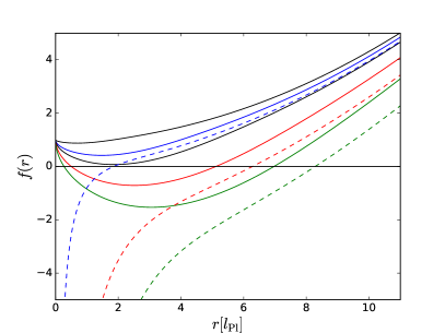
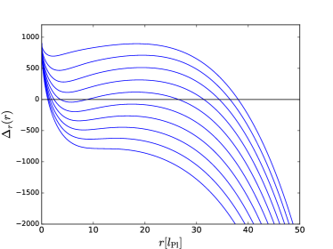
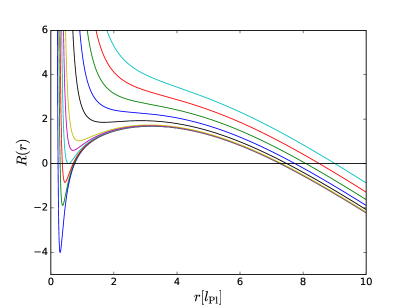
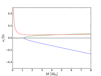
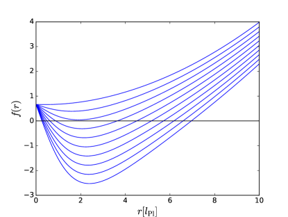
Classically, i.e. for constant & , the lapse function shows just one zero corresponding to the event horizon of the black hole, whereas the quantum improved Schwarzschild geometry shows up to two horizons, if a consistent matching is adopted, Figure 1. Starting at very large masses, well above the Planck mass, we find two horizons, generated by a minimum of the lapse function. Comparing with the classical lapse function in Figure 2 shows that the outer horizon of the quantum improved space-time coincides with the event horizon of the classical black hole. The larger the mass, the better the agreement and the more the inner horizon moves towards zero. Hence, increasing the mass makes the black holes more classical. Decreasing the mass causes the minimum to shrink and the horizons to move towards each other. There exists a critical mass around two Planck masses, , when the minimum is also a zero of the lapse function. Then, both horizons merge and has a double root. We will see later, that this geometry is similar to a classical, extreme Reissner-Nordström black hole in AdS. For masses below the critical mass, the minimum is above zero and no horizons are present.
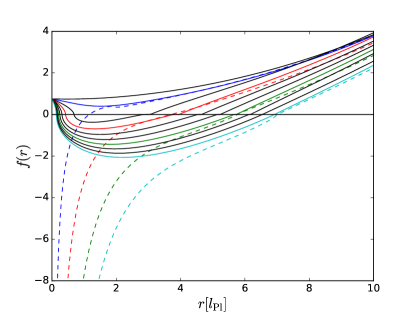
The results for matchings computed in space-times with running couplings agree with the matchings based on space-times with constant couplings on the position of the outer horizon, but differ significantly for smaller radii. These differences emerge because in the latter case, the matching is based on a classical geometry, whereas we actually study a quantum geometry with running couplings. Varying the amplitude for negative does not affect the qualitative results, but changes the scale.
V.2 Kerr-AdS
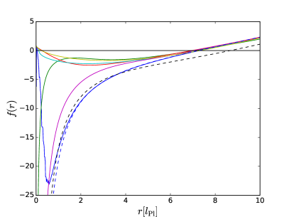
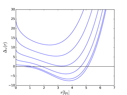
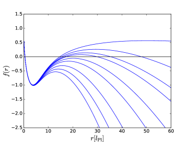
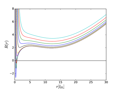
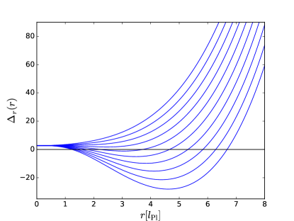
A classical, non-extremal Kerr-AdS space-time has two horizons: a Cauchy horizon inside the black hole event horizon. In contrast to the Schwarzschild case discussed above, the quantum improvement of this space-time does not allow for more horizons than in the classical geometry. Since the proper distances vanish identically in the consistent scenarios, we show only the results for the Kretschmann matching in Figure 3 and the dependence on the rotation parameter for fixed mass in Figure 4. The results for the linear matching can be found in appendix C. In general, the consistent quantum improved version displays the same behaviour as the classical solution. However, the inner horizon in the quantum improved space-time is located at larger radii than the classical Cauchy horizon, Figure 5.


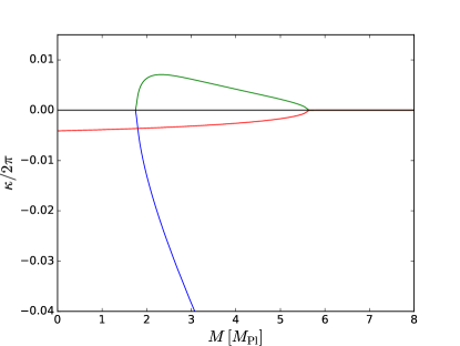
V.3 Asymptotically de Sitter spaces
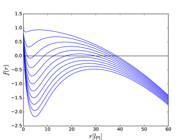
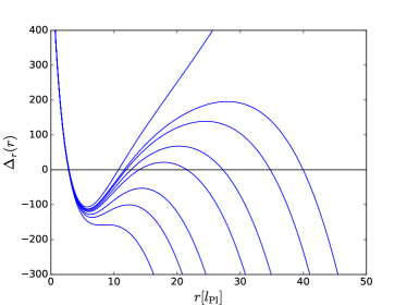
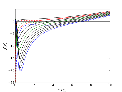
If we take the space-time to be asymptotically de Sitter, we find the possibility to get up to three horizons. The additional horizon is generated by the positive cosmological constant in the IR and appears in the classical regime at large radii. The typical shapes of and are displayed in Figure 6 & Figure 7 for the Kretschmann matching, the dependence on the amplitude of is shown in Figure 8 & Figure 9. Varying controls the position of the two inner horizons via the formation of a minimum, whereas governs the location of the outer horizon. Thereby, the interplay of the amplitudes of and dictates the number of horizons. Although we cannot provide an analytical condition involving and for the space-time exhibiting three horizons, it is suggestive to see it as the generalised version of the condition for a classical Kerr-dS space-time to have three horizons. This also implies that both quantum improved space-times have two distinct extremal cases: both inner horizons merge at a mass yielding an extremal black hole inside the cosmological horizon. Or both outer horizons merge at , forming the largest Schwarzschild/Kerr-dS black hole possible, analogous to the Nariai space-time.
VI Global Structure, Penrose Diagrams and Particle Trajectories
In contrast to the classical Schwarzschild-(A)dS and Kerr-(A)dS geometries of general relativity, the quantum improved counterparts can exhibit a different number of horizons and hence may show a different global structure, depicted in terms of Penrose diagrams. It turns out that both geometries, i.e. one based on the Schwarzschild and the other on the Kerr metric, have the same Penrose diagram. The resulting diagram is equivalent to the classical Reissner-Nordström or Kerr geometry. Hence, the quantum improvements of the metric lead to a unified global structure for quantum improved black hole space-times based on solutions of the Einstein field equations. Yet, as it is shown in section subsection VI.3 below, particles move differently in each geometry.
We start by determining whether the singularity is time-like, space-like or null. To that end we compute the norm of the normal vector of a hypersurface of constant in the limit . The norm turns out to be the -element of the inverse metric , yielding
| (12) |
Hence, the singularity is time-like in both cases, irrespective of whether the space-time is asymptotically AdS or dS. As it is shown in appendix B, zeros of and correspond to Killing horizons. The succession of sign changes of the lapse function dictates how the hypersurfaces of constant change from time-like over null to space-like.
VI.1 Asymptotically anti-de Sitter space-times
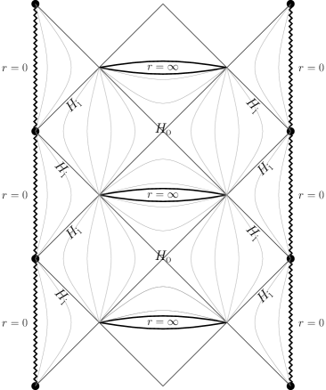
The lapse function of Schwarzschild-AdS and the Kerr-AdS space-time share the same qualitative features, resulting in the same Penrose diagram. The formal construction of the maximally extended space-time works the same as for the classical Kerr space-time, for instance see Carter (1968); Gibbons and Hawking (1977a), but now with an asymptotic AdS-patch. For a mass larger than the critical mass , the lapse function has two distinct roots, so the space-time exhibits two horizons, Figure 10. When , both roots coincide and we find an extremal black hole with just one horizon. For even lower masses, that is , no horizon is present, but the singularity still exists, cf. section VII, leaving a space-time with a naked singularity. Later, via a heuristic argument, we will argue that this unphysical space-time cannot be formed by gravitational collapse.
VI.2 Asymptotically de Sitter space-times
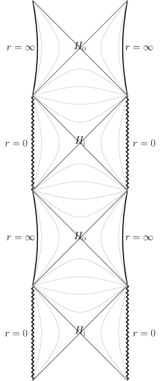
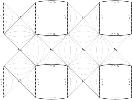
The results for the Schwarzschild- and Kerr-dS geometries agree with each other. The space-time exhibits two distinguished masses, , at which two of the possible three horizons merge. Starting with , the space-time has three distinct horizons, two of them are associated with the black hole and one with the positive cosmological constant on large scales, Figure 11. This case is equivalent to the classical Kerr-dS geometry. For , the outer black hole horizon and the cosmological horizon merge. This leaves an extremal space-time containing a maximally sized black hole, Figure 12, similar to the Nariai space-time. For even larger masses, there is just one horizon left, Figure 13. On the other end, the de Sitter space-time contains an extremal black hole if . For , we have a de Sitter geometry containing singularity, which is naked for observers within the cosmological horizon. The construction of the maximally extended space-time is analogous to the one for the classical Kerr-dS case, described for instance in Gibbons and Hawking (1977a).


VI.3 Particle Trajectories
In order to investigate whether particles propagate differently in the quantum space-times as compared to general relativity, we study their trajectories. Although most new effects in quantum improved space-times happen around the Planck scale, there are possibly deviations from classical trajectories already on length scales well above. Our set-up in the following is a test mass with zero angular momentum along its (timelike) geodesic in a non-extremal geometry, neglecting all backreactions. Furthermore, we are allowed to restrict the motion to the equatorial plane, see Hackmann et al. (2010) for more details. In order to classify orbits into categories, for instance orbits terminating at the central curvature singularity or bound ones, it suffices to study only the change of the radial coordinate.
VI.3.1 Schwarzschild
In the quantum improved Schwarzschild geometry, the equation for the radial motion of a test mass, starting with zero angular momentum at some distance with energy , reads according to (48)
| (13) |
where denotes the change of the radial coordinate along the geodesic parametrised by the eigentime. This equation is only dependent on and can be thought of as an energy equation per unit mass for the total energy of the test particle in an effective, one-dimensional potential . As was already found in Bonanno and Reuter (2000) for the asymptotically flat case, possible trajectories are the same as in the classical Reissner-Nordström scenario, thereby differing significantly from a classical Schwarzschild set-up. The only difference to the asymptotical flat case arises at large scales, where the effective potential , depending on whether the space-time is asymptotically de Sitter or anti-de Sitter. Recalling the shape of , e.g. Figure 1, we note that the effective potential is repulsive close to the singularity. In an asymptotically AdS geometry and for a test mass with energy , the following options are possible, all being bound orbits in radial direction:
-
1.
If equals the minimum of the lapse function , then the particle is on a circular, stable orbit in the region between the horizons. The radius is determined by the distance where the repulsive singularity balances the repulsive negative asymptotical cosmological constant.
-
2.
For , the particle is on a bound orbit, remaining in the region between both horizons.
-
3.
If , the orbit will again be bound, but now the particle periodically crosses horizons. For instance, first starting in the region outside of the outer horizon, the trajectory will first cross the outer horizon, then the inner one. Because it cannot overcome the repulsive barrier of the singularity, it is bounced back and the radius is increasing again. By crossing another horizon, it will end up in an identical patch of the extended space-time. This motion continues indefinitely and the particle will travel through infinitely many universes. We will comment on the physicality of this scenario at the end of this section.
-
4.
If , the energy of the particle can overcome the potential barrier and manages to approach the singularity at with non-zero kinetic energy. But in contrast to the classical Schwarzschild-AdS scenario, the particle again follows a path through infinitely many identical universes, reaching the singularity in each of them.
For the case of a non-extremal black hole with asymptotic de Sitter patch, we note that the maximum is always smaller than one. Therefore, we find scenarios one and two from above, but also some differences:
-
5.
The case admits a bound orbit, equivalent to scenario three with the outer turning point of the particle being located between the cosmological and the outer black hole horizon, as well as an unbound one beyond the cosmological horizon.
-
6.
For , the particle is at rest at the distance, where the attracting force of the black hole balances the attraction generated by the positive cosmological constant on large scales. This is an unstable equilibrium, since small perturbations cause the particle either to move inwards in a similar way to five, or to escape to infinity.
-
7.
In contrast to all above cases, the orbit is unbound in radial direction for , and the particle can escape to infinity. Depending on whether or not , it can reach the singularity at .
VI.3.2 Kerr
The equation for the change of the radial coordinate along the geodesic of a test particle with energy and zero angular momentum in the equatorial plane of the Kerr geometry reads (cf. (54)),
| (14) |
where we introduced the function for convenience. For a fixed geometry , the energy of the particle determines the allowed orbits. In the following, we continue closely along the more detailed analysis of the classical Kerr-(A)dS geometry carried out in Hackmann et al. (2010). Since the above equation is quadratic in , geodesics always have to satisfy . A simple root of corresponds to a turning point, where the particle comes to rest. A circular orbit of constant requires both and to vanish at , translating via equation (14) into the condition of having an extremum as well as a zero at . Depending on whether this extremum is a maximum or minimum, the circular orbit will be stable or unstable. Hence, having at least a double zero at is a sufficient condition for a circular orbit.
The function for Kerr-AdS is displayed in Figure 14. At large radii, the repulsiveness of the effective AdS space-time prevents particles from escaping to infinity. There exists a special energy , above which observers inevitably fall into the singularity along a terminating orbit. For , three types of orbits are possible. exhibits a double zero at , allowing for an unstable, circular orbit. For radii larger than , we find a bound orbit, crossing both horizons. Particles starting at are accelerated along terminating trajectories and will end up in the singularity. However, if , the double root splits and we find the possibility of having bound orbits as well as terminating ones at radii below the inner horizon. For the smallest energies, , the particle moves from horizon to horizon. The only difference for Kerr-dS compared to the AdS case, is that particles can always escape to infinity, see Figure 15.
The trajectories have been calculated for an idealised, pointlike observer, neglecting any backreaction on the geometry. However, the location of the inner horizon is typically at about the Planck scale, where backreaction effects should be taken into account. The quantum improved Schwarzschild case turns out to be similar to the classical Reissner-Nordström space-time, for which it was shown that there is a blueshift instability at the inner (Cauchy) horizon. Additionally, it was shown in Dafermos (2014), that perturbations of initial data cause the Cauchy horizon to be replaced by a null singularity. Due to the similarities between the quantum improved Schwarzschild and the classical Reissner-Nordström space-time, it is tempting to speculate that the classical findings might also hold for the quantum case. Hence, one has to take the above results with care, especially the many world trajectories. Summarising, there are differences between the classical and the quantum improved geometry, but they only become relevant at very small length scales, where the results have to be taken with a grain of salt.
VII Curvature Singularity & Effective Energy-momentum Tensor
Since quantum gravity effects become important in high curvature regimes, it is expected that they alter the nature of the curvature singularity at . Previous results from asymptotic safe quantum gravity Koch and Saueressig (2014b); Falls et al. (2012); Koch and Saueressig (2014a) and other quantum gravity scenarios, e.g. Modesto (2004), predict a substantial weakening of the singularity or even its disappearance. A weakening of the the singularity manifests itself for instance in changes of the Kretschmann scalar. We compute the Ricci scalar as well as the Kretschmann scalar of the quantum improved geometries in the UV fixed point regime, and compare the findings with the classical result of general relativity. Table 1 lists the highest degree of divergence of the Ricci and Kretschmann scalar for both investigated geometries for all discussed matchings. Upon comparison with the classical result of general relativity, the consistent quantum scenarios display a weakening of the singularity but not a complete resolution.
In the quantum improved space-times, the Ricci scalar is diverging too, because we have changed the geometry which is not a vacuum solution of the Einstein field equations anymore. In fact, it is a geometry with an effective energy-momentum tensor Cai and Easson (2011), induced by the running couplings. Using the classical field equations, this effective energy-momentum tensor can be computed by calculating the Einstein tensor from the quantum improved metric,
| (15) |
Note that is covariantly conserved, assuming a metric connection, , because the Einstein tensor satisfies the Bianchi identity by construction. However, physical interpretations of this effective energy-momentum tensor in terms of matter have to be drawn with great care. For instance, it turns out that the is diverging at horizons, , because and . Additionally, it has been shown in Reuter and Tuiran (2011), that in the quantum improved flat Kerr geometry violates the weak, the null, the strong and the dominant energy condition. We expect similar results in the present case, including the cosmological constant. These observations suggest that quantum gravity contributions to the energy-momentum tensor are of a fundamentally different nature than the ones of conventional matter and should not be interpreted as matter. In fact, the running couplings should be taken into account already on the action level, resulting in different field equations. This is done for example in Quantum Einstein Gravity (QEG) Reuter and Saueressig (2012), based on the quantum improved Einstein Hilbert action
| (16) |
The resulting new field equations Reuter and Weyer (2004b), based on the runnings (3), read the same as (15) with
| (17) |
It has been shown in Koch and Ramirez (2011), that the covariant conservation of the effective energy-momentum tensor in QEG is equivalent to the following relation between the running couplings,
| (18) |
This relation is not satisfied by our quantum improved Schwarzschild-(A)dS and Kerr-(A)dS metrics, meaning that they are not solutions to the new field equations (15) with (18), derived in the Einstein-Hilbert truncation of a potentially more complicated fundamental action.
| classical | cl. Kretschmann | qu. Kretschmann | linear | cl. radial path | qu. radial path | cl. geodesic | qu. geodesic | |
|---|---|---|---|---|---|---|---|---|
VIII Horizon Temperatures and Black Hole Evaporation
In this section, we first establish the fact, that surface gravities in space-times based on the quantum improved version of the radial path proper distance are divergent, before discussing the Hawking temperatures in the Kretschmann scenario. Finally, we will discuss implications on the black hole evaporation process.
The Hawking temperature of a black hole in flat space received by an observer at infinity is given by Hawking (1975), with surface gravity of the event horizon. For an observer at finite distance in the static region outside the black hole, the above expression is modified by a redshift factor,
| (19) |
where is the norm of the static Killing vector . In more general terms, a surface gravity can be assigned to any Killing horizon of a space-time. Gibbons and Hawking showed in Gibbons and Hawking (1977a), that cosmological horizons also emit radiation which can be detected by an observer in the static space-time region. In general, emission is a consequence of the observer not being able to access the space-time hidden behind the horizon(s), thereby being fundamentally unable to measure the quantum state of the complete universe (see Gibbons and Hawking (1977a) for a more detailed discussion). The notion of a horizon temperature only appears to be meaningful for observers in a static space-time region, since only such observers detect radiation of this temperature. Taking Reissner-Norström as example, this is only the case for the region outside the black hole. In between the horizons, the space-time is not static anymore and inside the inner horizon, the space-time is static again, but connected to the singularity. This would require to impose boundary conditions at the singularity, being far from obvious. Hence in the following, we only refer to a horizon having a temperature, if the horizon is the boundary of a static region, not connected to the singularity. In appendix B, horizons in the quantum improved space-time are shown to be Killing horizons, thus a surface gravity can be assigned to each of them.
Technically, the surface gravity of a Killing horizon can be computed by taking the covariant derivative of the norm of the Killing vector, or alternatively via a periodicity in Euclidean time introduced in Gibbons and Hawking (1977b). In any case, we find
| (20) |
being the radial coordinate of the horizon. Since horizons are zeros of and respectively, (36) implies that the derivative of the proper distance diverges at the horizons for the quantum version of the radial path. As addressed in appendix D in detail, this does not necessarily mean that the proper distance itself is diverging at a horizon, unless the horizon is extremal. But computing the surface gravity explicitly via (20) generates the following terms, proportional to , and therefore diverging at the horizons,
| (21) |
The terms in the brackets are in general non-vanishing at the horizons. In particular, this holds also for arbitrary large masses in the classical regime, where it is known that the surface gravity and Hawking temperature stays finite. This is the main reason why we consider the scale identification based on the quantum radial path as unphysical. In contrast, along with the proper distance based on a geodesic, the construction based on the Kretschmann scalar shows no divergent behaviour at the horizons and therefore leads to finite Hawking temperatures.
Next, we discuss the mass dependence of the surface gravities, focusing on the quantum Kretschmann scenario from now on. It suffices to look at the slope of the lapse function at each horizon, since it is proportional to the surface gravity. The results for Schwarzschild-AdS and Schwarzschild-dS can be found in Figure 16 and Figure 17, the plots for the Kerr cases are qualitatively the same. The whole evolution, appearance and disappearance of horizons is driven by the formation of a minimum of the lapse function. The quantum improved Schwarzschild-AdS space-time exhibits no horizon up to the critical mass . At , the minimum of the lapse function is at zero, hence the slope is zero and so are the surface gravities. For growing mass, the slope becomes steeper because the minimum expands, thus the surface gravities grow in amplitude. In contrast, in general relativity diverges for . However, the surface gravity of the outer horizon matches the classical one for sufficiently large masses. The Schwarzschild-dS scenario can have up to three horizons and two special masses, and , at which two of the three horizons merge. Starting in the regime, there is no black hole, but only the cosmological horizon. The case corresponds to the case from above. For , there are three horizons and the back hole gets bigger for increasing mass, until , when the black hole has reached its maximal size and its outer horizons merges with the cosmological horizon to an extremal horizon with zero temperature.
In AdS space-times, an observer in the static region could only
measure a temperature coming from the black holes’ event horizon,
whereas in dS space-times, the observer would measure a mixture of two
thermal spectra at different temperatures, one coming from the back hole and
one from the cosmological horizon. In the static region outside the
black hole, one valid choice for the Killing vector in
(19) is , yielding
. In the Schwarzschild geometries, this implies that an
observer located at a horizon would measure an infinite temperature,
in accordance with general relativity. In Schwarzschild-AdS, the
temperature drops to zero for an infinitely distant observer, as
diverges.
In the dS-scenario, there exists a distance between
the horizons, at which the observed temperature becomes minimal, s
because has a maximum. In
the Kerr geometries, is timelike only outside
the ergoregion. A static Killing vector field for the entire region
outside the black hole can be obtained by linearly combining the two
Killing vectors of a Kerr space-time, see appendix
B. Since all above observations equally apply
for classical as well as quantum improved space-times, the is no
qualitative difference for an observer measuring horizon temperatures
in a classical or a quantum space-time, except in the Planckian
regime.
As final point, we would like to address the black hole evaporation process. A standard mechanism to form black holes is gravitational collapse. If the mass of a collapsing object is larger than the Tolman-Oppenheimer-Volkoff mass around , no other force can counterbalance gravity and the object collapses to form a black hole. Assuming that a macroscopic Schwarzschild or Kerr black hole has formed via this process, well above the critical mass, it will emit Hawking radiation and thereby lose energy. This causes the black hole to shrink steadily, as its mass is decreasing. This process continues, until the critical mass is reached. The temperature then becomes zero and therefore the radiation stops. Hence, the naked singularity case with can never be reached via this process and we end up with a zero temperature, Planck-sized, extremal black hole, often referred to as remnant. This remnant serves as shield, guaranteeing that the cosmic censorship conjecture remains satisfied. However, in Aretakis (2015) it was shown that extremal black hole configurations with zero temperature suffer from an instability at the extremal horizon. Remnant endpoints were also found in other studies within asymptotic safety Bonanno and Reuter (2006); Falls et al. (2012) and beyond Chen et al. (2015). Based on a classical expression for the proper distance it has been shown in Koch and Saueressig (2014a, b) that the Schwarzschild-AdS black hole evaporates completely. A more suitable set-up to discuss the evaporation process is given by the dynamical Vaidya space-time, used in Bonanno and Reuter (2006). There, a Planck-sized, cold remnant as endpoint has been found.
IX Summary
In this work, the quantum improved Kerr-(A)dS black hole was studied for the first time within a self-consistent scale identification procedure. The latter is based on the Kretschmann scalar. The Kerr-(A)dS geometry also includes the Schwarzschild-(A)dS, as well as ordinary Schwarzschild and Kerr space-times as special cases, by setting either the rotation parameter or the cosmological constant to zero.
Both quantum improved geometries show the same global structure in terms of a timelike curvature singularity at and the same number of horizons. Furthermore, it has also been shown that the outer black hole horizon corresponds to the classical black hole event horizon. The timelike character of the singularity at in principle allows particles to avoid the singularity. The quantum corrections to the classical metric render the singularity less divergent, but none of the studied scenarios was able to resolve it completely. However, this singularity will always be dressed by a horizon, such that there is no violation of the cosmic censorship conjecture.
The horizons being Killing horizons admit a temperature, causing the black hole to evaporate. In the Planckian regime, however, the heat capacity of a tiny black hole stays positive, , in contrast to the classical case. Thus, the evaporation process comes to an end when the Hawking temperature of the black hole is zero, leaving an extremal, cold, Planck-sized remnant, serving as cosmic censor. This is a thermodynamically stable endpoint, because any additional mass absorbed by the black hole will radiate away until the temperature is again zero. It would be interesting to see what implications for the black hole information paradox can be drawn from the generic existence of such remnants.
Acknowledgements.
We thank Alfio Bonanno, Kevin Falls, Domenico Giulini and Alessia Platania for discussions. This work is supported by EMMI and is part of and supported by the DFG Collaborative Research Centre ”SFB 1225 (ISOQUANT)” and also by the DFG Research Training Group ”Models of Gravity”.
Appendix A Choice of Scale Identification
Here we motivate our choice for in (5). Inserting the general parametrisation , into (37), we are left with
| (22) | ||||
The numerical values of and depend on the particular RG-trajectory and parametrisation we have chosen and therefore cannot be physical observables. However, the product is an observable and hence independent of the particular choice of the RG-trajectory. Its magnitude turns out to be , e.g. in Reuter and Saueressig (2012); Denz et al. (2018). In this light, we have two choices for in order to make (22) solely dependent on ,
| (23) |
Thus, in (5) we have chosen the second of the two equivalent options. Varying for a fixed geometry (), which is effectively done also in the quantum Kretschmann scenario by introducing , turns out to have only a weak impact on the position of the inner horizon. Since it is typically located at small radii, we recall from Table 2, that varying mildly modifies the UV-limit. Furthermore, we have an upper limit .
Appendix B Killing Horizons
In this section, we review the formal proof that every zero of in (7) is a Killing horizon. This implies that a constant surface gravity and thereby a temperature can be associated to each horizon. The Schwarzschild-(A)dS case is automatically contained by taking .
Starting from the Kerr-(A)dS metric (7), assume that has positive roots, i.e. can be written as
| (24) |
The horizons are the hypersurfaces . Since the space-time is axisymmetric and stationary, we have two commuting Killing vector fields: is stationary, at least in some region of the space-time, and manifests the symmetry axis. We now have to construct a Killing vector field , that is normal to, and null on these horizon hypersurfaces. The most general form for would be a linear combination of both Killing vector fields,
| (25) |
with a constant . We will fix this constant later by requiring that should vanish at the horizons. But first, we must change from Boyer-Lindquist coordinates (7), to coordinates that leave the metric regular at the horizons. Such coordinates are induced by the principal null directions of the space-time. The Kerr-(A)dS space-time is of algebraic type D, thus admits two distinct principal null directions, referred to as ingoing and outgoing. They can be represented in Boyer-Lindquist coordinates by the following vectors,
| (26) |
where is outgoing and ingoing. They now induce outgoing and ingoing coordinates, being the Kerr-(A)dS counterparts of Kerr-coordinates in flat space. We will select the outgoing version, but in principle we could also work with ingoing ones. The outgoing Kerr-(A)dS coordinates are defined as,
| (27) |
Inserting these back into (7), leaves us with the metric in terms of Kerr-(A)dS coordinates ,
| (28) |
One can check that (28) reduces to Kerr coordinates for . The Killing vector field now reads
| (29) |
Requiring that is null on the horizons yields
| (30) |
and therefore
| (31) |
Thus, we have found a family of vector fields , being null at one horizon at a time. In order to show that the hypersurfaces are Killing horizons, it remains to be checked if is hypersurface orthogonal, i.e. evaluated at the horizon,
| (32) |
with all other components vanishing. In summary, we are able to construct a Killing vector field which is null on, and normal to each horizon hypersurface , and hence have shown that the horizons corresponding to the roots of are indeed Killing horizons.
Appendix C Other Matchings
C.1 Linear Matching
The simplest scaling is based on a dimensional analysis,
| (33) |
which has already been adopted for instance in Bonanno and Reuter (2000). In the case of an identically vanishing cosmological coupling, is the IR-limit of the classical proper distance along a radial path Falls et al. (2012). But this matching does not take physical scales of the underlying space-time into account, for instance the black hole scales given by & , or scales induced by the gravitational or the cosmological coupling. Nevertheless, this function already gives rise to many phenomena observed for more complicated choices and hence can serve as a toy model.
C.2 Proper Distances
We can also use the proper distance along a curve in space-time to specify ,
| (34) |
This definition is diffeomorphism invariant and encodes the space-time structure, since the gravitational and cosmological coupling typically appear in the metric. In most cases in the literature, e.g. Koch and Saueressig (2014b); Falls et al. (2012); Koch and Saueressig (2014a), the gravitational as well as cosmological coupling have been fixed to be constants, for instance the IR-values and . However, since the FRG-flow generically gives rise to running couplings, it is more natural and consequent to consider this running also in the above integral, thus and . In the following, this quantum improvement procedure of proper distances is extended to Schwarzschild- and Kerr-(A)dS geometries. We will provide expressions for the proper distance along a radial path and along the geodesic of a radially infalling observer, both for constant, as well as running and . Additionally, the UV-limit of each proper distance is obtained, cf. Table 2.
C.2.1 Radial Path
Inspired by the symmetry of the space-time, we first take the following radial path from to as integration contour in (34),
| (35) |
The restriction to the equatorial plane in the Kerr case is done for the sake of simplicity. Driven by the results of Reuter and Tuiran (2011) for the flat Kerr geometry, we assume that the varying will not alter our results qualitatively. Applying the above integration paths to (34) yields,
| (36) |
with the lapse functions
| (37) |
In the following, this scenario with constant and will be referred to as classical radial path, because the space-time underlying the integral is a classical black hole geometry with a cosmological constant.
Alternatively, we account for the running of the couplings already in the proper distance, referred to as quantum radial path with and in the above integrals. This turns (36) into integral equations for , which can be transformed into a differential equation by taking a derivative with respect to . One can then easily see that the derivative of diverges at every horizon, where and vanish. Using the fixed point behaviour of and in the UV, these differential equations read for small ,
| (38) |
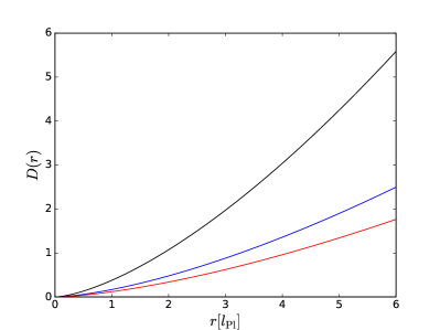
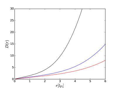
Both classical matchings as well as the one for the quantum Schwarzschild scenario monotonously increase and satisfy , as can be seen from the numerical results in Figure 23. In contrast, the proper distance is identically zero in the quantum Kerr scenario, see (42).
It turns out (cf. section VIII), that the expression for the Hawking temperature in a quantum improved space-time contains terms proportional to the derivative of , hence using the above construction for the proper distance leads to diverging Hawking temperatures at all horizons. Therefore, in the following we also discuss the proper distance induced by the eigentime of a radially infalling observer, where this feature is absent.
C.2.2 Radial Timelike Geodesic
The eigentime of an observer, initially at rest at and falling along a radial timelike geodesic into the singularity, can also be used to identify the momentum cut-off scale with a length scale by setting . Derived in appendix F, the eigentime for the Schwarzschild-(A)dS scenario reads
| (39) |
with for an observer initially starting at rest. It is worth noting that for , the integral reduces to the one in (36). By fixing , we equivalently specify the maximal distance of the observer from the origin. Independent on the particular value of , the proper distance again exhibits poles if , now shifted by away from the horizons. Once more, (39) gives rise to two different proper distances, referred to as either classical or quantum geodesic, depending on whether the underlying space-time is based on the constant or running versions of and . ss The analogous expression for the proper distance induced by an radial geodesic in the Kerr-(A)dS scenario reads (see appendix G)
| (40) | ||||
and reduces to (36) for . Again, we achieved that there are no poles at the horizons. Once more, we have two versions depending on whether and are running or not. The numerical results can be found in Figure 24, however, the proper distance in the quantum Kerr scenario is again identically zero.
| Kretschmann | Radial Path | Geodesic Path | ||||
|---|---|---|---|---|---|---|
| classic | quantum | classic | quantum | classic | quantum | |
| Schwarzschild | ||||||
| Kerr | ||||||
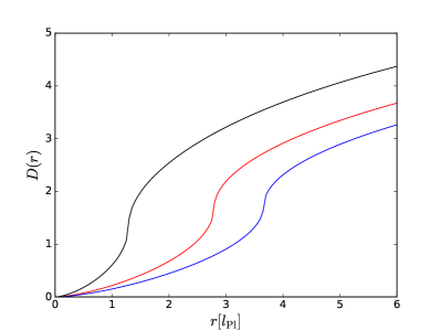
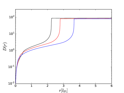
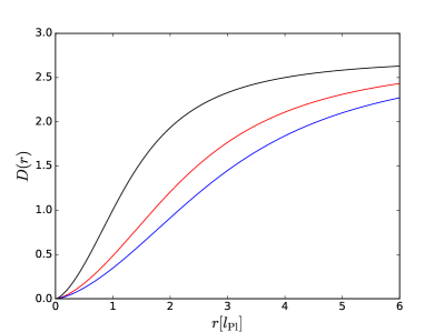
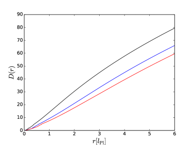
Appendix D Shape and Divergences of Proper Distances
As can be seen from Figure 23-25, all functions are monotonously increasing, some proper distances display a rapid increase. In order to understand these jumps and possible divergences, we have to look at the integral expressions for each proper distance (36), (39), and (40). The expression under each square root can become zero, and if has just a single root at , the corresponding pole is integrable, causing a jump in the proper distance,
| (41) | ||||
where has no root at . However, once the multiplicity of is larger than one, the pole is not integrable anymore and exhibits a divergence at . In any case, is diverging for the radial path proper distances, even at integrable poles of , as can be seen from (38). In case of the classical radial path, the position of these poles has no direct physical significance, however in the quantum case, the poles are located precisely at the horizons, because then, the function is nothing other than the horizon condition. Thus, for extremal black holes when at least two horizons coincide, the quantum proper distance along a radial path is ill-defined. is always diverging at the horizons leading to a diverging Hawking temperature of the horizon, as is shown in section VIII.
For this reason, we introduce the scenario with an infalling observer along a timelike, radial geodesic, in order to remove these problems, only due to the poor choice of the function and absent in all other scenarios. However, it turns out, that in both proper distance scenarios for Kerr-(A)dS with an underlying quantum space-time, the proper distance must vanish identically, in order to satisfy the condition . For instance, this can be seen by solving (38) in the limit , satisfying the boundary condition , yielding
| (42) |
Therefore, the solution vanishes identically in the limit , which is confirmed also for the full, numerical solution of (36). The same behaviour is found for Kerr-(A)dS, when the scale matching is based on the geodesic in a quantum-improved space-time.
Appendix E UV-limits of D(r)
For statements about the curvature near the singularity and also for the construction of the Penrose diagrams, the UV-limit for each proper distance is needed.
The leading order behaviour in the UV for the classical proper distances, i.e. constant and , can be obtained from (36), (39) and (40) by approximating the integral in the limit . For the identification based on the classical Kretschmann scalar (10), the UV-behaviour can easily be read off from (11).
In the quantum versions, the leading order of the proper distance in the UV-limit can be obtained by assuming a power law behaviour of the form , with constants and in order to satisfy the boundary condition . The constants and can be determined by inserting this ansatz back into the above equations, now being an integral, differential or functional equation respectively. All scenarios display monotonously increasing functions satisfying , apart from the quantum proper distance expressions for Kerr. They are identically zero, as an iterative algorithm for solving the integral equations shows.
For each scenario, the analytical UV-expression is listed in Table 2. The numerical results for are shown in Figure 23, Figure 24, Figure 25. Furthermore, the leading order exponent can be extracted numerically from the slope of the linear relation between the proper distance and its integral function :
| (43) |
This cross-check confirms agreement between numerical exponent and the one found analytically in Table 2.
Appendix F Eigentime of an Inflating Observer in a Schwarzschild-(A)dS Geometry
Another physically well-motivated choice for the integration path in (34) is the curve determined by an observer some distance away from the black hole, falling into the black hole along a radial timelike geodesic. Because the observer’s four-velocity is conserved along geodesics, we normalise it to be
| (44) |
Furthermore, we can choose the coordinate system such that the motion takes place only in the equatorial plane . Using (6), the normalisation condition of the four-velocity in the equatorial plane reads:
| (45) |
where denotes the derivative with respect to the eigentime . We have also conserved quantities and corresponding to the Killing vector fields and :
| (46) | ||||
| (47) |
However, for simplicity, we will choose an observer with . Inserting and back into (45) to eliminate and leaves us with
| (48) |
This is a type of energy equation for the observer, at least in asymptotically flat spacetimes. We now have to specify the initial conditions for the observer. In the asymptotically flat spacetime, one usually places the observer initially at rest at , still leaving finite. However, we cannot do that in the case of a non-vanishing cosmological constant, because is diverging for . Therefore, we take rather an observer at rest () at some finite distance to determine :
| (49) |
The proper distance is then given by the eigentime the observer needs to arrive at after starting at , i.e the integral over the eigentime along the geodesic:
| (50) |
Appendix G Eigentime of an Inflating Observer in a Kerr-(A)dS Geometry
Following the same procedure for a timelike geodesic in the equatorial plane in Kerr-(A)dS, given by the metric (7), the normalisation of the four-velocity is
| (51) |
whereas the conserved quantities induced by the Killing vector fields and read
| (52) | ||||
| (53) |
Combining the equations and restricting again to yields the following radial equation,
| (54) |
Subsequently, we arrive at the proper distance in a Kerr-(A)dS geometry induced by an infalling observer in the equatorial plane, initially starting at rest at and falling towards the singularity at :
| (55) |
where is in this case then given by
| (56) |
References
- Weinberg (1979) S. Weinberg, General Relativity: An Einstein centenary survey, Eds. Hawking, S.W., Israel, W; Cambridge University Press , 790 (1979).
- Reuter (1998) M. Reuter, Phys. Rev. D57, 971 (1998), arXiv:hep-th/9605030 .
- Bonanno and Reuter (1999) A. Bonanno and M. Reuter, Phys. Rev. D60, 084011 (1999), arXiv:gr-qc/9811026 [gr-qc] .
- Bonanno and Reuter (2000) A. Bonanno and M. Reuter, Phys. Rev. D62, 043008 (2000), arXiv:hep-th/0002196 .
- Reuter and Tuiran (2011) M. Reuter and E. Tuiran, Phys. Rev. D83, 044041 (2011), arXiv:1009.3528 [hep-th] .
- Koch and Saueressig (2014a) B. Koch and F. Saueressig, Class. Quant. Grav. 31, 015006 (2014a), arXiv:1306.1546 [hep-th] .
- Falls et al. (2012) K. Falls, D. F. Litim, and A. Raghuraman, Int.J.Mod.Phys. A27, 1250019 (2012), arXiv:1002.0260 [hep-th] .
- Koch and Saueressig (2014b) B. Koch and F. Saueressig, Int. J. Mod. Phys. A29, 1430011 (2014b), arXiv:1401.4452 [hep-th] .
- Bonanno et al. (2017) A. Bonanno, B. Koch, and A. Platania, Class. Quant. Grav. 34, 095012 (2017), arXiv:1610.05299 [gr-qc] .
- Bonanno and Reuter (2006) A. Bonanno and M. Reuter, Phys. Rev. D73, 083005 (2006), arXiv:hep-th/0602159 .
- Falls and Litim (2014) K. Falls and D. F. Litim, Phys. Rev. D89, 084002 (2014), arXiv:1212.1821 [gr-qc] .
- Reuter and Weyer (2004a) M. Reuter and H. Weyer, Phys. Rev. D70, 124028 (2004a), arXiv:hep-th/0410117 [hep-th] .
- Emoto (2005) H. Emoto, (2005), arXiv:hep-th/0511075 [hep-th] .
- Niedermaier (2007) M. Niedermaier, Class. Quant. Grav. 24, R171 (2007), arXiv:gr-qc/0610018 .
- Litim (2011) D. F. Litim, Phil.Trans.Roy.Soc.Lond. A369, 2759 (2011), arXiv:1102.4624 [hep-th] .
- Reuter and Saueressig (2012) M. Reuter and F. Saueressig, New J. Phys. 14, 055022 (2012), arXiv:1202.2274 [hep-th] .
- Bonanno and Saueressig (2017) A. Bonanno and F. Saueressig, Comptes Rendus Physique 18, 254 (2017), arXiv:1702.04137 [hep-th] .
- Percacci (2017) R. Percacci, An Introduction to Covariant Quantum Gravity and Asymptotic Safety, 100 Years of General Relativity, Vol. 3 (World Scientific, 2017).
- Eichhorn (2017) A. Eichhorn, in Black Holes, Gravitational Waves and Spacetime Singularities Rome, Italy, May 9-12, 2017 (2017) arXiv:1709.03696 [gr-qc] .
- Denz et al. (2018) T. Denz, J. M. Pawlowski, and M. Reichert, Eur. Phys. J. C78, 336 (2018), arXiv:1612.07315 [hep-th] .
- Dittrich and Reuter (1985) W. Dittrich and M. Reuter, Effective Lagrangians in Quantum Electrodynamics (Springer Verlag, 1985).
- Gibbons and Hawking (1977a) G. W. Gibbons and S. W. Hawking, Phys. Rev. D 15, 2738 (1977a).
- Hindmarsh and Saltas (2012) M. Hindmarsh and I. D. Saltas, Phys. Rev. D86, 064029 (2012), arXiv:1203.3957 [gr-qc] .
- Copeland et al. (2015) E. J. Copeland, C. Rahmede, and I. D. Saltas, Phys. Rev. D91, 103530 (2015), arXiv:1311.0881 [gr-qc] .
- Carter (1968) B. Carter, Phys. Rev. 174, 1559 (1968).
- Hackmann et al. (2010) E. Hackmann, C. Lammerzahl, V. Kagramanova, and J. Kunz, Phys. Rev. D81, 044020 (2010), arXiv:1009.6117 [gr-qc] .
- Dafermos (2014) M. Dafermos, Commun. Math. Phys. 332, 729 (2014), arXiv:1201.1797 [gr-qc] .
- Modesto (2004) L. Modesto, Phys. Rev. D70, 124009 (2004), arXiv:gr-qc/0407097 [gr-qc] .
- Cai and Easson (2011) Y.-F. Cai and D. A. Easson, Phys. Rev. D84, 103502 (2011), arXiv:1107.5815 [hep-th] .
- Reuter and Weyer (2004b) M. Reuter and H. Weyer, JCAP 0412, 001 (2004b), arXiv:hep-th/0410119 [hep-th] .
- Koch and Ramirez (2011) B. Koch and I. Ramirez, Class. Quant. Grav. 28, 055008 (2011), arXiv:1010.2799 [gr-qc] .
- Hawking (1975) S. W. Hawking, Comm. Math. Phys. 43, 199 (1975).
- Gibbons and Hawking (1977b) G. W. Gibbons and S. W. Hawking, Phys. Rev. D15, 2752 (1977b).
- Aretakis (2015) S. Aretakis, Adv. Theor. Math. Phys. 19, 507 (2015), arXiv:1206.6598 [gr-qc] .
- Chen et al. (2015) P. Chen, Y. C. Ong, and D.-h. Yeom, Phys. Rept. 603, 1 (2015), arXiv:1412.8366 [gr-qc] .