Robustness of Magic and
Symmetries of the Stabiliser Polytope
Abstract
We give a new algorithm for computing the robustness of magic—a measure of the utility of quantum states as a computational resource. Our work is motivated by the magic state model of fault-tolerant quantum computation. In this model, all unitaries belong to the Clifford group. Non-Clifford operations are effected by injecting non-stabiliser states, which are referred to as magic states in this context. The robustness of magic measures the complexity of simulating such a circuit using a classical Monte Carlo algorithm. It is closely related to the degree negativity that slows down Monte Carlo simulations through the infamous sign problem. Surprisingly, the robustness of magic is submultiplicative. This implies that the classical simulation overhead scales subexponentially with the number of injected magic states—better than a naive analysis would suggest. However, determining the robustness of copies of a magic state is difficult, as its definition involves a convex optimisation problem in a -dimensional space. In this paper, we make use of inherent symmetries to reduce the problem to dimensions. The total run-time of our algorithm, while still exponential in , is super-polynomially faster than previously published methods. We provide a computer implementation and give the robustness of up to 10 copies of the most commonly used magic states. Guided by the exact results, we find a finite hierarchy of approximate solutions where each level can be evaluated in polynomial time and yields rigorous upper bounds to the robustness. Technically, we use symmetries of the stabiliser polytope to connect the robustness of magic to the geometry of a low-dimensional convex polytope generated by certain signed quantum weight enumerators. As a by-product, we characterised the automorphism group of the stabiliser polytope, and, more generally, of projections onto complex projective 3-designs.
1 Introduction
In fault-tolerant quantum computation (for a recent review, see Ref. [8]), each logical qubit is encoded in a non-local subspace of a number of physical qubits. There are several ways of effecting a unitary transformation of logical qubits. In the simplest case, logical unitaries can be implemented transversally, i.e. by local gates acting on the physical qubits. Unfortunately, a no-go theorem by [13] states that there are no quantum codes that allow for a universal set of transversal gates.
In the magic state model [5], the logical gate set is chosen to be the Clifford group, which can be implemented transversally in various quantum codes using their physical counterparts. Any logical non-Clifford gate would promote the Clifford group to universality. This remaining problem is solved by providing an auxiliary qubit in a non-stabiliser state. Using a circuit gadget (which only requires Clifford operations), one can turn this auxiliary state into a non-Clifford gate (Fig. 1). The auxiliary qubit state is consumed in the process, so that one such input needs to be injected for each non-Clifford gate. These inputs are the magic states from which the protocol derives its name.

A common choice for a non-Clifford gate is the -gate , which is realised by the following magic state
| (1) |
Moreover, there is a second magic state, , which realises the non-Clifford gate . Their Bloch representation is shown in Fig. 5. Interestingly, it has been found that even certain mixed states can “supply the magic” to promote a Clifford circuit to universality. Indeed, a process called magic state distillation (Fig. 2) can turn many copies of some mixed state into a pure magic state using Clifford unitaries and computational basis measurements [5, 34].
Magic state distillation motivates the search for quantitative measures of the “computational utility” of auxiliary states. This analysis turns out to be slightly simpler for quantum systems with odd-dimensional Hilbert spaces [36, 27, 37], as the theory of stabiliser states is somewhat better-behaved in this case, and there is a better-developed toolbox of “phase space methods” available in this case (see e.g. Refs. [15, 42, 24]). However, as qubits are the paradigmatic systems for quantum computation, quantitative resource theories for multi-qubit magic states have since been developed [23, 6].
The starting point of these theories is the Gottesman-Knill Theorem [30]. It states that quantum circuits consisting only of preparations of stabiliser states, Clifford unitaries, and computational basis measurements can be efficiently simulated on a classical computer. Therefore, if the auxiliary states are stabilisers, there can be no quantum computational advantage. Next, assume that an auxiliary -qubit state is an element of the stabiliser polytope , i.e.
where is a probability distribution and the are stabiliser states. This readily gives rise to an efficient classical randomised algorithm that will draw outcomes from the same distribution as a quantum computer would [39], provided that one can sample efficiently from the probability distribution : Indeed, draw with probability , and then continue to simulate the further time evolution using Gottesman-Knill. Thus, density matrices contained in the convex hull of stabiliser states are equally useless as computational resource states in the magic state model (Fig. 3).
Since the stabiliser states span the space of Hermitian operators, any auxiliary state can be expanded as , with coefficients that are not necessarily non-negative. However, taking traces on both sides shows that the expansion is affine, i.e. . It is well-known in the theory of Quantum Monte Carlo methods [17] that the probabilistic algorithm sketched above can be extended to the more general scenario. However, the runtime will increase with the total amount of “negativity” in the expansion coefficients . This is the dreaded sign problem. A precise theory of the simulation runtime in the context of quantum computation has been developed in Ref. [31] and applied to the magic state model in Ref. [23]. More precisely, they define the robustness of magic (RoM) as
| (2) |
where the sum ranges over stabiliser states and the -norm
measures the “amount of negativity” in the affine combination. Then, the number of samples which have to be taken in the Monte Carlo simulation scales as [23, 31].
In addition to measuring the “computational utility” in the above precise sense, the RoM has further interpretations. For example, it can be used to systematically lower-bound the number of non-Clifford gates required to synthesise certain unitaries, namely those that allow for a magic state realisation [23]. Lastly, the RoM derives its name from the fact that it quantifies the robustness of a state’s computational utility against noise processes. A precise account of this point of view is given in Section 2.
Interestingly, the RoM is submultiplicative, i.e. , where the inequality is usually strict [23]. That means that the simulation effort of a magic state circuit grows subexponentially with the number of injected magic states—an intriguing phenomenon. Therefore, a quantity of interest is the regularised RoM:
Unfortunately, computing seems to be a difficult task. For being a single-qubit state, the tensor power lives in an -dimensional space, and the sum over the in the definition (2) of the RoM has to range over the stabiliser states defined for -qubit systems. Any direct implementation of the optimisation problem (2) will thus quickly became computationally intractable—and, indeed, [23] could carry it out only up to .
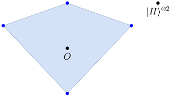
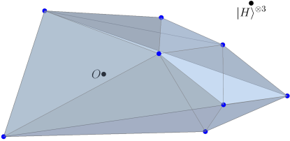
The starting point of this work is the observation that there is a large symmetry group shared by and the stabiliser polytope. Thus, we formulate the optimisation in a space where the joint symmetries have been “modded out”. The space of operators invariant under the joint symmetry group turns out to have a dimension mildly polynomial in . For the especially interesting cases where the state is or , the dimension reduces further to exactly . While the projection of the stabiliser polytope to this invariant space (Fig. 4) still has exponentially many vertices, it turns out that formulating the optimisation problem in this symmetry-reduced way leads to a super-polynomially faster algorithm.
Equipped with the knowledge of the exact solution to Eq. (2) for the commonly used magic states and and qubits, we formulate a relaxation of the RoM problem for these states which yields an upper bound for the exact RoM. These approximations are in excellent agreement with the exact data for and can be carried out for up to qubits. What is more, we can not only compute the RoM bounds for these approximations, but also find the corresponding affine decompositions , which can directly be used in Monte Carlo simulations. Furthermore, we find a hierarchy of such RoM approximations by restricting to -partite entangled stabiliser states which converges to the exact RoM. Interestingly, every level of the hierarchy can be computed in polynomial time.
Finally, both the exact and approximate results imply a runtime of for simulating a circuit with T gates using the RoM algorithm. Moreover, our analysis suggests that this runtime is the optimal one that can be achieved using a RoM algorithm. Our work improves on the previously known runtime of derived in Ref. [23]. Note that the RoM algorithm is able to simulate noisy circuits and mixed states. This is in contrast to simulation algorithms based on the so-called stabiliser rank which can achieve a runtime of for pure states [4, 6, 7].
This paper is organised as follows. Section 2 is devoted to a short discussion of the Robustness of Magic, giving an alternative definition to the one in the previous section and stating the properties of this resource monotone. Next, a series of techniques is presented which use the symmetries in the definition of the monotone to simplify the computation significantly. To this end, the symmetry group of the stabiliser polytope is characterised in Sec. 3.2 and certain classes of states are singled out in Sec. 3.3 which profit from a high degree of symmetry. For these states, we explicitly derive the symmetry-reduced problem by constructing a suitable basis for the invariant subspace in Sec. 3.3, followed by enumerating equivalence classes of stabiliser states up to symmetry in Sec. 3.4. The numerical solutions for the constructed problems are presented and discussed in Section 4. Based on this, we prove a polytime relaxation of the RoM problem in Sec. 4.3. Our results are summarised in Sec. 5.
2 Robustness of Magic
The resource theory of magic states can be developed in analogy to the more-established resource theory of entanglement and the robustness of entanglement [38] studied in this context. There, the robustness of a state can be interpreted as a measure for the worst-case separable noise that renders the state separable. However, its construction can be generalised to any resource theory as follows: Given a convex set of free resources, the robustness of relative to is defined as
| (3) |
Depending on the choice of , the robustness might be infinite. If it is finite, we can express as a pseudo-mixture
| (4) |
Following [38], one can define the so-called total robustness by minimising over the set of free resources:
| (5) |
In the following, we choose to be the convex polytope spanned by the -qubit stabiliser states. More precisely, , where is the set of all -qubit stabiliser states. Here, and in the following, by a “quantum state”, we will always mean the density matrix representing it. In the case of pure states , the associated vector will be referred to as a state vector. The polytope is a subset of the real vector space of -dimensional Hermitian matrices where is the overall dimension of Hilbert space. More specifically, quantum states lie in the -dimensional affine subspace given by . Within this affine hyperplane, is full-dimensional and we usually consider it as the the ambient space of .
[23] work with an equivalent robustness measure: the robustness of magic (RoM) introduced in Eq. (2). A straightforward calculation (c.f. Appendix A) shows that the two measures are related by a simple affine transformation:
| (6) |
The robustness of magic provides a proper resource monotone with the following properties:
Proposition 1 (Properties of Robustness of Magic [23]).
The robustness of magic has the following properties:
-
1.
Faithfulness: iff
-
2.
Monotonicity: for all stabiliser operations with equality if is unitary.
-
3.
Convexity: for .
-
4.
Submultiplicativity: .
3 Exploiting stabiliser symmetries
3.1 Definition of the RoM problem.
The Robustness of Magic is defined as the following optimisation problem.
Problem 1 (Robustness of Magic).
Let be the set of stabiliser states. Given a state , solve the following problem:
| min | |||
| s. t. |
Using standard techniques, this problem can be reformulated as a linear program (LP) with constraints and variables [3]. Although the time complexity of LPs is linear in the product of number of constraints and variables, these numbers themselves grow super-exponentially with the number of qubits . Concretely, and . Moreover, the LP needs access to an oracle which provides the stabiliser states. The implementation of such an oracle would necessarily have super-exponential time complexity itself. However, even if an efficient oracle were provided, the storage of the states would quickly exceed the memory capacity of any computer. In practice, this limits the evaluation of the problem to on normal computers and renders it infeasible, even on supercomputers, for .111Already the storage of would require around 77 TiB of memory. For , this number increases to around 76 PiB which exceeds the state-of-the-art by a factor of 7.
A standard method in the analysis of optimisation problems is dualising the problem. Clearly, by Slater’s condition, strong duality holds and thus the dual problem is an equivalent definition for the Robustness of Magic. In Appendix B, we state the dual problem and derive a lower bound from a feasible solution. However, this bound matches the one that was already found in Ref. [23].
3.2 Symmetry reduction
The complexity of the RoM problem can be significantly reduced by exploiting the symmetries of the problem, a procedure that we will call symmetry reduction and is well-known in convex optimisation theory, see e. g. [2]. Here, we will explain the basic ideas and refer the interested reader to App. E for a mathematical review.
By stabiliser symmetries , we mean the linear symmetry group of the stabiliser polytope. This is the group of linear maps that leave invariant. These maps necessarily have to preserve the set of vertices, i. e. the set of stabiliser states . Clearly, the group of -qubit Clifford unitaries induces such symmetry transformations by conjugation. Another obvious symmetry of the set of stabilisers is the transposition:
where is the (anti-unitary) operation of complex conjugation in the computational basis. The group of unitary and anti-unitary operations generated by Clifford unitaries and complex conjugation is known as the extended Clifford group [1]. Our first result states that any stabiliser symmetry is induced by the action of an element of the extended Clifford group on the Hilbert space. This is a corollary of the more general Thm. 1 on symmetries of 3-designs and is proven in App. C.
Corollary 1.
The group of stabiliser symmetries is given by the adjoint representation of the extended Clifford group .
We emphasise that this is a non-trivial result which is in general wrong for the case of odd-dimensional qudits where it is possible to construct explicit counter-examples. This turns out to be related to the fact that stabiliser states fail to form 3-designs in odd dimensions [41, 25, 40].
Note that anti-unitary symmetries in act in the adjoint representation as , where and is the transposition map. Hence, there are only global antiunitary symmetries. Every tensor product of local antiunitary symmetries would involve a partial transposition and such a map could not preserve the set of entangled stabiliser states.
Let be a (not necessarily maximal) subgroup fixing . The projection onto the subspace of -fixed points , see App. E, is given by
| (7) |
Note that is trace-preserving, hence the image of quantum states will again lie in the affine subspace .
Recall that we can express the robustness of as a minimisation over and (mixed) stabiliser states such that
| (8) |
Since preserves , every such decomposition yields a decomposition in terms of -invariant mixed stabiliser states:
| (9) |
In particular, if the decomposition was optimal in the first place, the projected decomposition is also optimal.
This shows that there is always -invariant optimal solution for the problem. Hence, instead of optimising over the whole set of stabiliser states, we only have to optimise over -invariant mixed stabiliser states . By Lemma 3 in App. E, these are exactly given by and can thus be computed by evaluating the projections . Since for all and , it is sufficient to compute the projections on representatives of . Finally, we remark that a majority of the projected states are not extremal points of the projected polytope . Given an extremal subset , the symmetry-reduced version of Prob. 1 is given by substituting and .
3.3 Identification of symmetries
The first step towards the explicit symmetry-reduced problem is to identify the group that fixes the state of interest. Motivated by magic state distillation and the submultiplicativity problem, we are especially interested in the case with being a -qubit state. A large part of the analysis does not depend on the choice of , so we keep the discussion as general as possible and specialise later to and particular choices of . The symmetries of can be classified as follows:
-
Permutation symmetry Clearly, is invariant under permutations of the tensor factors. Such permutations also preserve the stabiliser polytope. Thus, the symmetric group is contained in the symmetry group of the problem.
-
Local symmetries By local symmetries of we mean products of -qubit stabiliser symmetries of . By Corollary 1, this class contains only local Clifford operations. Let be the stabiliser of within the -qubit Clifford group , then the local symmetry group is given by .
-
Global symmetries We refer to all other symmetries as global. The global symmetry group contains e.g. the transposition .
The maximal symmetry group for is given by the subgroup that stabilises within . Here, we focus on the subgroup of which is given by local symmetries and permutations:
| (10) |
The following analysis suggests that for our choices of , actually coincides with , meaning that there are no further global symmetries. However, since the study of symmetries in can be quite involved [16], we can not exclude the possibility that we missed some of the symmetries.
For the rest of this paper, we will consider the case . Note that acts by rotating about the symmetry axes of the stabiliser polytope. It is easy to see that states with non-trivial stabilisers fall into three classes: Stabiliser states (with trivial robustness), and magic states that lie on the Clifford orbit of or . Since the RoM is Clifford-invariant, we can pick the following states for concreteness:
| (11) |
Figure 5 shows the two states and their stabiliser symmetries. The respective unitary symmetries correspond to a two-fold rotation symmetry about the -axis and three-fold rotation symmetry about the -axis. In terms of Clifford operations, these stabiliser groups are represented by
| (12) |
Recall that these should be understood in the adjoint representation and thus the order of these groups is indeed and .
Furthermore, there are antiunitary stabiliser symmetries
| (13) | ||||||||
| (14) | ||||||||
| (15) |
such that is fixed by and and is fixed by and . Recall that these can only contribute global symmetries such as . However, the common eigenspace of and coincides with that of and thus adding these symmetries to the symmetry group will not further reduce the invariant subspace. A similar argument holds also for the antiunitary symmetries of .
Hence, the considered symmetry groups are as follows:
| (16) |
Since the symmetric group is always a subgroup of the symmetry group, the fixed point subspace is always a subspace of the totally symmetric subspace . Let us first consider a generic state with no further symmetries. Then, coincides with . Thus, the trace 1 subspace has dimension and is thus exponentially smaller than the full space. A basis for the symmetric subspace is given by a Fock-style “occupation number basis” constructed from the Pauli basis as follows
| (17) |
Here, the symmetrisation operator is given by averaging over all permutations of the tensor factors. The trace one subspace can be obtained as the span of all basis elements with the component set to .
Due to linearity, the symmetrisation map is completely determined by its action on the Pauli basis. Given a Pauli operator , there is a permutation such that . The appearing exponents , and are exactly the weights of , i. e. the number of , , factors, respectively. By the invariance of under permutations, we thus get . We define weight indicator functions,
| (18) |
such that we can write the -projection of a Pauli operator as
| (19) |
By extending the functions linearly to , we thus get exactly the coefficients of the projection in the number basis.
Let be a stabiliser group stabilising a state . The projection of this state is
| (20) |
The are the coefficients of the complete signed quantum weight enumerators of the stabiliser code . Recall that for a classical code , the complete weight enumerator is the degree- polynomial in variables given by
where gives the number of times appears in [26]. The analogy should be clear. Unsigned weight enumerators for quantum codes have been studied since the early days of quantum coding theory [28, Ch. 13]. Much less seems to be known about their signed counterparts, with Refs. [33, 32] being the only related references we are aware of. There it is shown that, as their classical analogues, signed quantum weight enumerators are NP-hard to compute.
Finally, we want to return to the cases and and discuss the invariant subspaces for these states. Let us rotate the Pauli basis such that the first basis vector corresponds to the Bloch representation of and , respectively:
| (21) | ||||||
| (22) | ||||||
| (23) |
Note that this choice of basis is such that the orthogonal decompositions of state space correspond to (real) irreps of the respective Clifford stabilisers , as can be seen from the matrix representation of the generators in the rotated basis:
| (24) |
In general, a basis for the trivial representation of in the -qubit state space is given by . To construct a basis for the full invariant subspace, we have to symmetrise resulting in . Here, is the occupation number basis associated to the rotated basis and is constructed analogously to before.
In general, the components of stabiliser states in the rotated bases can be written in terms of weight enumerators by computing the induced basis transformations on from to . However, we are only interested in the projection onto which simplifies this computation. First, let us rewrite the -qubit Pauli operators in the -basis. Note that every operator with non-vanishing -weight is already in the orthocomplement of .
| (25) |
Here, we left out possible identity factors and all orthogonal terms on the RHS, i. e. those containing . This result implies that we can write the projection of a stabiliser state as
| (26) |
We call the numbers the partial signed quantum weight enumerators of . The analysis works the same way for the -projection:
| (27) |
In this case, the -projection of a stabiliser state with stabiliser group involves total signed quantum weight enumerators as follows:
| (28) |
Note that all projections , and can be computed from the complete signed weight enumerators of the stabiliser codes which themselves are functions of the weight distributions. For numerical purposes, it is convenient to absorb all appearing factors in the bases such that the coefficients of stabiliser states are given by the integer weight enumerators.
Finally, we want to give expressions for the states and in the respective bases:
| (29) | ||||
| (30) |
In general, we are not aware of any method which can predict whether the projection of a stabiliser state will be extremal within the projected polytope. However, the following lemma gives a necessary condition on the extremality of products of stabiliser states which will be useful later.
Lemma 1 (Projection of product states).
The following is true for : If the projection of an arbitrary stabiliser state is non-extremal, so is for any other stabiliser state .
Proof.
We prove the statement by showing it on the level of the complete signed weight enumerators . This proves the claim directly for and the other cases follow since the partial and total signed weight enumerators are linear functions of the complete ones.
Note that the Pauli , , weights are additive under tensor products, e. g. . This implies that we can write the indicator function as for , , being the weights of . However, since is zero if , , are not the weights of , we can instead sum over all possible decompositions on the right hand side. Hence, for any two stabiliser codes we get
| (31) |
Suppose is the stabiliser of a state and can be written as convex combination,
| (32) |
with stabiliser states , stabilised by the groups . Let be stabilised by , then we find by Eq. (31),
| (33) |
and hence the projection of the product state is non-extremal. ∎
Note that Eq. (31) allows us to compute the projection of products from and via the signed quantum weight enumerators using operations. This is an important improvement over computing for a general (fully entangled) stabiliser state which requires operations.
3.4 Representatives of inequivalent stabiliser states
Computing the projected polytope involves the computation of the signed quantum weight enumerators for all stabiliser states. However, from the previous discussions we know that we can restrict the computations to the orbits with respect to the symmetry group In this section we will construct representatives for these orbits.
Our approach is based on a subset of the set of stabiliser states, the so-called graph states . For every simple, i. e. self-loop free, graph of vertices, there is a state vector that is stabilised by operators of the form
| (34) |
where are the Pauli operators on the -th qubit and is the adjacency matrix of the graph . Graph states play a fundamental role in the studies of stabiliser states since [35] proved that every stabiliser state is equivalent to a graph state under the action of the local Clifford group :
| (35) |
This result can be used to label every stabiliser state vector by a local Clifford unitary and a graph state such that . However, -equivalent graph states generate the same -orbit and are equally well suited to represent a stabiliser state. [29, 19] discovered that that two graph states are -equivalent if and only if the underlying graphs are related by a graph theoretic transformation called local complementation (LC). Thus, it is sufficient to consider graphs up to local complementation.
Furthermore, the symmetry group induces additional equivalence relations on the graph state representation. Let us again begin the discussion with the case of a generic state with -symmetry. This already allows us to restrict the representation to non-isomorphic graphs, i. e. graphs up to permutation of their vertices, since for any graph state and a permuted version the -orbits are isomorphic: with the permuted local Clifford unitary . Moreover, it is straightforward to show that the composition of graph isomorphism and local complementation is symmetric and thus a equivalence relation on graphs whose equivalence classes are isomorphic to . These equivalence classes have been studied in the context of graph codes and entanglement in graph states [11, 20] and were enumerated by [10]. However, different local Clifford unitaries can still result in equivalent states. To see this, pick some symmetry of the graph, i. e. , then the actions of and yield isomorphic states. Hence, it is enough to act with on the graph state .
For the computation of the -orbits it is enough to consider , since Pauli operators will only change the possible signs of the final generators which are better added by hand. It is well known that the quotient is isomorphic to the binary symplectic group which is the foundation of the phase space formalism. We make use of this formalism to compute the -orbits of graph states by evaluating the orbits of the local symplectic group up to the stabiliser of and .
The additional symmetries in the case of the and state can be taken into account by restricting the allowed symplectic transformations using the symplectic maps and induced by the generators and , respectively. The corresponding cosets are given by the representatives and , respectively.
However, the described generation procedure will quickly become computationally expensive. Moreover, most of the projected stabiliser states are non-extremal points for the projected polytope and thus redundant. Unfortunately, there is no simple way of deciding whether a state will be extremal after projection or not. However, Lemma 1 states at least a criterion for product states which allows us to restrict to projecting only fully entangled stabiliser states. To this end, we only have to iterate over connected graph representatives with respect to and compute the projections of product states directly from lower-dimensional vertices using the appropriate version of Eq. (31).
4 Computing the robustness of magic
Using the enumeration procedure of the last section, we generated the set of - and -projections of fully entangled stabiliser states and the set of projected product states from lower-dimensional vertices. In an additional step, we removed non-extremal points from the set of projected states, resulting in vertex sets of the projected stabiliser polytopes for and , respectively. As described in the last section, we are labelling the vertices by certain stabiliser representatives. To this end, we use a notation in terms of “decorated graph states” compatible with Refs. [35, 14]: A graph is decorated by symbols which indicate the action of local Clifford operations on the respective graph state. Nodes with signs indicate a sign change of the respective stabiliser generator, or alternatively, the action of on the respective qubit prior the any other gates. A hollow node in the graph denotes a Hadamard gate acting on the respective qubit and self-loops correspond to the action of phase gates (prior to possible Hadamard gates). Figure 6 shows the vertex sets for . Since the dimension of the polytope is exactly , it can be easily visualised for , see also Fig. 4 in Sec. 2.
The database of vertices and the program code can be found on the arXiv [21]. For a discussion of the algorithmic details see App. D.


| + prod. | + prod. | ||||
| 1 | 6 | 3+0 | 2 | 2+0 | 2 |
| 2 | 60 | 5+3 | 4 | 4+3 | 4 |
| 3 | 1080 | 11+8 | 8 | 4+8 | 6 |
| 4 | 36720 | 48+18 | 13 | 18+14 | 12 |
| 5 | 2423520 | 252+38 | 32 | 61+26 | 22 |
| 6 | 315057600 | 1881+86 | 60 | 256+57 | 42 |
| 7 | 81284860800 | 20378+208 | 144 | 2151+116 | 66 |
| 8 | 41780418451200 | 331794+510 | 304 | 21475+226 | 131 |
| 9 | 42866709330931200 | 8410183+1270 | 804 | 329712+462 | 238 |
| 10 | – | – | – | 5964000+991 | 371 |
Table 1 shows the number of vertices of the projected polytopes in comparison with the original number of stabiliser states. We see that the number of states that have to be used in the -minimisation is reduced drastically from to a scaling which is approximately . Additionally, the dimension of the ambient space is reduced exponentially from to exactly . As discussed in Sec. 3.2, the required -minimisation for RoM is computed via a linear program with constraints and variables and has a runtime that is linear in its size . The runtime is thus reduced as
| (36) |
leading to a super-polynomial speed-up in the -minimisation. Although both time and space complexity of the -minimisation are exponential in , it is in principle feasible for moderate . Here, the limiting factor is the implementation of the oracle providing the projected states with runtime which is still super-exponential in .
4.1 Robustness of the and states
Figure 7 shows the Robustness of Magic of for , computed from the vertices of the projected stabiliser polytope. Note that the data for is in perfect agreement with the so-far computed values in Ref. [23]. We are particularly interested in the submultiplicative behaviour of . Here, the new data for turns out to be helpful: We can observe that the data points quickly approach an apparent exponential scaling with . More precisely, submultiplicativity is clearly observable for , but the scaling becomes effectively multiplicative for larger . We quantified this using an exponential fit of the data range (shown in blue in Fig. 7) resulting in . From previous works it is known that the regularised robustness is bounded from below by 1.207. Our work, however, indicates that it converges from above to a constant which is given by the fit as .
| 1 | 1.41422 | 1.41422 |
|---|---|---|
| 2 | 1.74754 | 1.32195 |
| 3 | 2.21896 | 1.30432 |
| 4 | 2.86274 | 1.30076 |
| 5 | 3.68705 | 1.29818 |
| 6 | 4.73894 | 1.29603 |
| 7 | 6.07646 | 1.29405 |
| 8 | 7.78935 | 1.29252 |
| 9 | 9.97501 | 1.29119 |
The previously known time complexity for simulating a circuit with T gates using the RoM algorithm is [23]. Our findings improve this to . Moreover, since we already explored an effectively multiplicative regime of the RoM, solving the problem for higher will not much reduce the runtime. From our estimate for the asymptotic regularised robustness, we can estimate the best possible scaling to be .
Furthermore, we applied the same procedure to compute the robustness of the magic state . Since the -symmetry group is larger than in the previous case, we were able to compute for up to 10 qubits, see Fig. 8. Qualitatively, the results agree very well with those of the last section. Quantitatively, the robustness of the state is considerably higher than the one of the state. Using again an exponential fit, we find the scaling which predicts a regularised robustness of . By the RoM construction, the 10-qubit solution gives rise to a simulation algorithm with runtime where is the total number of magic states used, or equivalently, the number of -rotation gates.
| 1 | 1.73206 | 1.73206 |
|---|---|---|
| 2 | 2.23206 | 1.49401 |
| 3 | 3.09808 | 1.45780 |
| 4 | 4.33100 | 1.44260 |
| 5 | 6.04494 | 1.43311 |
| 6 | 8.35898 | 1.42460 |
| 7 | 11.5114 | 1.41772 |
| 8 | 15.8436 | 1.41248 |
| 9 | 22.1823 | 1.41110 |
| 10 | 30.7056 | 1.40839 |
4.2 Analysis of the optimal solutions
Additionally, we studied the optimal solutions of the -minimisation for the previously discussed cases of and . For this purpose, it is instructive to use the original formulation of the robustness of a state in terms of an optimal affine combination of two (mixed) stabiliser states , cp. Eq. (5):
| (37) |
The states can be obtained from the optimal solution of the -minimisation as follows:
| (38) |
Recall from the discussion in Sec. 3.2 that replacing every vertex in the optimal solution by a stabiliser representative in its preimage yields an optimal solution for the original problem. Hence, we simply identify the vertices of the projected polytope by their stabiliser representatives constructed in Sec. 3.3. Surprisingly, these states seem to have a rather simple structure, especially the positive contributions . We will discuss the solutions in the following for the and case separately.
Optimal solutions for the state
The positive contributions to the state for are simply given by the graph state . Figure 9 shows the remaining states for . Note that these states have to lie on a facet of the polytope to minimise the robustness. But instead of the generic contributions, they can be written using only terms. The vertices themselves are products of and the Bell state .

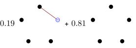


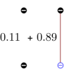

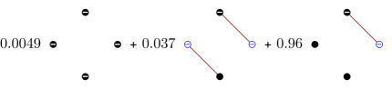


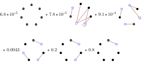
In contrast, the negative contributions , shown in Fig. 10, have less structure and seem to be partially irregular. Of course, has a non-unique convex combination and thus part of structure could be shadowed by the non-uniqueness. Nevertheless, since the dominant part of the contributions consists of products of and the Bell states , it is reasonable to assume that the can be approximated by Bell states. We suspect that this approximation is quite good, at least for a moderate number of qubits, due to the apparent suppression of vertices with more complex structure.
Motivated by these observations, we define the following polytope:
| (39) |
By Eq. (31), we can compute these states efficiently from the signed weight enumerators of and . Note that the projection of is a convex combination of the projected Bell states and thus only states with “all plus” or “all minus” contributions are extremal in . Let be the set of vertices of and . We can explicitly enumerate its elements by tuples such that . Every such tuple corresponds to a product of , and states. Hence, the number of vertices is
| (40) |
We define the approximate robustness of as the robustness with respect to the polytope :
| (41) |
Since the optimisation is over a subset of all projected stabiliser states, is an upper bound for . Moreover, it can be efficiently evaluated since both the complexity of computing and of the -minimisation is . Figure 11 shows a comparison of with the exact robustness. From the previous analysis it is clear that the approximation is exact for . The deviation from the exact data for is at most 0.06% and thus negligible. However, we expect that the deviation becomes larger the higher is, since it is likely that the importance of multipartite entangled contributions increases. Nevertheless, the approximation seems to be surprisingly good. The approximate data again follows an exponential increase with , predicting an asymptotic regularised robustness of about which is compatible with the prediction from the exact data.
However, this approach is limited to . For larger , the -minimisation lacks a feasible solution, which can only be the case if is not in the affine span of the product states . This indicates that the dimension of the subpolytope becomes too small. A solution to these infeasibility problems will be discussed in Sec. 4.3.
| 1 | 1.41422 | 1.41422 |
|---|---|---|
| 2 | 1.74754 | 1.74754 |
| 3 | 2.21896 | 2.21896 |
| 4 | 2.86274 | 2.86274 |
| 5 | 3.68705 | 3.68930 |
| 6 | 4.73894 | 4.74071 |
| 7 | 6.07646 | 6.07650 |
| 8 | 7.78935 | 7.78942 |
| 9 | 9.97501 | 9.97510 |
Optimal solutions for the state
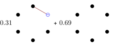
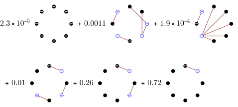
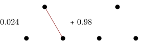
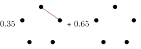
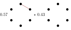
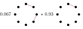
As in the previous case, the two connected vertices of the projected 2-qubit polytope constitute a dominant part in the optimal solutions. They are not projections of Bell states, so we will denote their representatives by and define them to be the states stabilised by and , respectively. The analysis of the optimal solutions shows that the states are convex combinations of products of and the maximally entangled state . Moreover, they seem to be even more sparse than for the previous case, see Fig. 12. As in the case of , the state shows only partial structure, see Fig. 14 .


| 1 | 1.73206 | 1.73206 |
|---|---|---|
| 2 | 2.23206 | 2.23206 |
| 3 | 3.09808 | 3.09808 |
| 4 | 4.33100 | 4.33316 |
| 5 | 6.04494 | 6.04494 |
| 6 | 8.35898 | 8.36006 |
| 7 | 11.5114 | 11.5117 |
| 8 | 15.8436 | 15.8492 |
| 9 | 22.1823 | 22.2499 |
| 10 | 30.7056 | 30.9411 |
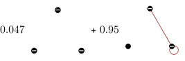




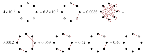
The similarities suggest that the robustness for can be well approximated using a similar procedure as in the last section. To this end, we define the polytope
| (42) |
The approximate robustness is again defined with respect to this polytope. The vertices can be efficiently computed using the same procedure as in the case and the approximation is exact for . Figure 13 shows the approximate robustness compared to the exact results. The approximation is again surprisingly good with a maximum deviation from the exact data of around 0.8%. Although this error is still small, it is an order of magnitude larger than for the state. The approximation yields an asymptotic regularised robustness of which is slightly larger than the result from the exact data. Similar to the last section, the applicability of this approximation is limited to due to the infeasibility of the optimisation problem for larger . In the next section, we will show how to generalise this approximation to overcome the feasibility problems.
4.3 Finite hierarchy of RoM approximations
In general, the idea of restricting to at most -partite entangled stabiliser states leads to a hierarchy of approximations with levels . Clearly, for the exact problem is recovered. The set of at most -partite entangled -qubit stabiliser states can be constructed by taking all possible tensor products of states in for which result in -qubit states. However, without the presence of additional symmetries, this will still result in an exponentially large set since already the set of fully separable stabiliser states () has size .
Hence, we assume that we want to compute approximations to where is a symmetric -qubit state (not necessarily pure) such that the stabiliser symmetry group contains at least the symmetric group . In particular, this applies to the magic states and . In this case, we are able to give upper bounds on the runtime for every fixed level .
Following Lemma 1 and Section 3.3, the set of -projections of -partite entangled -qubit stabiliser states can be constructed from the vertices of the projected polytopes for which have fully entangled representatives. Let us denote the sets of representatives by . Since the order does not matter, the possible ways to take tensor products of these sets are exactly captured by (descending) partitions of into parts with size at most . We will denote such a partition by . Then, we define the subpolytope of projected -partite entangled states as
| (43) |
and the -th level of the RoM hierarchy by the relaxation of Prob. 1 to the subpolytope . Clearly, this defines an upper bound to the exact RoM .
To bound the runtime of the -th level of the hierarchy, we have to count the vertices of . An upper bound to this number is given by the number of tensor products appearing in Eq. (43) up to permutations. Thus, let be a (descending) partition of into parts, with no part larger than :
| (44) |
This can be rewritten as
| (45) |
where is the multiplicity of in the partition . Since the permutations of the partition itself were already considered, the number of product states corresponding to the partition is given, up to permutations, by
| (46) |
Using that the number of fully entangled vertices is increasing with , we can bound this number by
| (47) |
Finally, the number of partitions of with parts no greater than coincides with the number of partitions of into at most parts and is denoted by . A standard result in number theory is that
| (48) |
Thus, we can bound the number of vertices to be
| (49) |
Since the dimension is , this implies that the runtime of the relaxation of Problem 1 is polynomial in for a fixed .
Finally, we remark that one has to know the vertex sets up to to run the -th level of the hierarchy. Moreover, the bounds are very loose due to the fact we have not strictly bound the number of fully entangled vertices which is beyond the scope of this paper. However, by using the actual numbers for , one can obtain much better bounds on by evaluating the binomial coefficients. Let us illustrate this for the case of and : Using that , and , we find
| (50) | ||||
| (51) |
Note that we derived in the previous section using further information about the extremality of products.
5 Conclusion & Outlook
In this work, we have studied the symmetries of the -qubit stabiliser polytope and showed how to use these to greatly reduce the combinatorical complexity of computing the robustness of single-qubit magic states and to gain insight into the structure of the problem.
We have determined the symmetry groups for the two types of single-qubit magic states and have constructed explicit stabiliser state representatives of the symmetry orbits. This has allowed us to evaluate the robustness of for and for qubits. Using the structure of the solutions, we have proposed an approximation based on at most bipartite entangled states which is efficient in and gives an upper bound on the exact robustness. Furthermore, the agreement with the exact data for qubits is excellent. Since the RoM becomes effectively multiplicative for larger , we expect that the approximation is still very good in the regime . Moreover, by restricting to -partite entangled stabiliser states, we obtained a finite hierarchy of approximations which recovers the exact RoM for . We showed that a fixed level of the hierarchy can be computed in time.
We feel that the most interesting task left open in this work is to explain why even two-body entangled states are sufficient to produce excellent bounds on the RoM. This may be insightful in a wider context. Indeed, sub-additivity of resource costs occurs in several areas of quantum information theory, most famously for the entanglement of formation [18]. The violations to additivity in [18] can be proven to exist for randomised constructions in high dimensions. This makes it hard to study the structure of the optimal solutions, or their behavior in a limit of many copies. The combinatorial nature of the stabiliser polytope, and the observation that only few-body entanglement is enough to find almost-optimal solutions, suggest that RoM may provide an instance where understanding submultiplicativity is feasible.
6 Acknowledgements
We thank Earl Campbell, Mateus Araújo, Felipe M. Mora, Felix Huber, Frank Vallentin, Arne Heimendahl, and Huangjun Zhu for helpful discussions and comments. In particular, we want to thank Richard Kueng for productive discussions concerning the dual problem.
This work has been supported by the Excellence Initiative of the German Federal and State Governments (Grant ZUK 81), the German Research Foundation (DFG project B01 of CRC 183), and ARO under contract W911NF-14-1-0098 (Quantum Characterization, Verification, and Validation).
Appendix A Equivalence of the two robustness measures
[38] defined the so-called total robustness which is given by
| (52) |
For being a (compact) polytope, this can be rewritten as follows. Since is compact, the minimum is attained. Hence, and
| (53) |
Let be the vertices of and write as convex combinations with coefficients and . It follows:
| (54) |
The last sum is an affine combination of the vertices since . In other words, is a feasible solution for the following minimisation problem:
| (55) |
Moreover, the optimal value can be bounded as follows:
| (56) |
Assume is the optimal solution for . Then, we can rewrite , using , as follows:
| (57) |
Hence, the optimal affine combination for becomes
| (58) | ||||
| (59) |
Here, the renormalised modulus of the affine coefficients form a convex combination and hence . Thus, we found a pseudo-mixture for and the parameter can not be smaller than the total robustness of :
| (60) |
Combined with Eq. (56), this shows that the two measures are equivalent:
| (61) |
Finally, let us remark that constructed from the optimal affine combination for is such that
| (62) |
Appendix B On the dual RoM problem
At this point, any analytical insight could be helpful in simplifying the problem. A standard method is dualising the problem. Clearly, by Slater’s condition, strong duality holds and thus the dual problem is an equivalent definition for the Robustness of Magic. The dual problem is straightforwardly obtained as follows:
Problem 2 (Dualised Robustness of Magic).
Let be the set of stabiliser states. Given a state , solve the following problem:
| max | |||
| s. t. |
This formulation of the RoM has a particularly nice form. Thus, it seems at first that the dual problem might be easier to solve. Indeed, one can guess the following feasible solution:
| (63) |
Here, denote the -qubit Pauli operators which generate the -qubit Pauli group . Feasibility follows from the following calculation for a stabiliser state with stabiliser group :
| (64) |
The corresponding objective value is
| (65) |
where is the coefficient vector of in the Pauli basis, i.e. . The objective value yields a lower bound to the RoM of . Note that this bound, also called st-norm , was already found in [23] with different techniques and gives the following lower bound on the RoM of and :
| (66) |
Appendix C Symmetries of 3-designs
In this section, we characterise the symmery group associated with the projectors of certain -designs.
A complex projective -design is a finite family of unit vectors in such that
| (67) |
where
| (68) |
is the orthogonal projection onto the totally symmetric subspace . Furthermore, is its dimension and acts by permuting the factors of the tensor product . Taking a partical trace of Eq. (67) shows that a -design is also a design.
As in the main part of this paper, we denote by the real vector space of Hermitian matrices with the induced Hilbert-Schmidt inner product . With respect to this inner product, we denote by the adjoint of a linear map and call orthogonal if it preserves the inner product, or equivalently, if .
Theorem 1.
Let be a set of unit vectors. Let be a linear map on Hermitian operators that permutes the projectors .
-
1.
If is a 1-design, then is unital (i.e. ).
-
2.
If is a 2-design, then is orthogonal and trace-preserving.
-
3.
If is a 3-design, then is of the form , where is either a unitary or an antiunitary operator on .
Proof.
Define .
1.—Using , we get
| (69) |
hence is unital.
2.—Let us define the traceless operators operators . Using the fact that forms a 2-design, Eq. (68), and the “swap trick”
| (70) |
valid for the non-trivial element of , one verifies the following for any traceless Hermitian operator :
| (71) |
In other words, the operators form a tight frame for the subspace of traceless Hermitian matrices. Moreover, setting with , a similar calculation shows that the set forms a tight frame for all of .
By 1., is unital and thus permutes the tight frame . However, any map permuting the elements of a tight frame is orthogonal. Finally, orthogonal and unital maps preserve the trace:
| (72) |
3.—Consider the following trilinear function on :
| (73) |
is invariant under since is also a symmetry of the projectors :
| (74) |
We can explicitely evaluate by expanding in terms of permutations and arguing as in Eq. (70). This yields
| (75) |
The first four terms are individually -invariant since preserves the trace and is orthogonal. Hence, the -invariance of implies
| (76) |
Since this holds , we get
| (77) |
A linear automorphism on a matrix algebra fulfilling (77) is called a Jordan automorphism. Our goal is to apply a known structure theorem that restricts that form of such maps [22]. For the theorem to be applicable, we have to extend from a map on the real vector space of Hermitian matrices, to a map on the algebra of all matrices. To this end, we use that every can be written uniquely as where , and set
| (78) |
Clearly, this continuation yields a linear automorphism on . Morover, since the anticommutator is bilinear, we get :
| (79) |
i. e. the continuation to is a Jordan automorphism. It is also straightforward to check that orthogonality of implies that is unitary with respect to the trace inner product.
It is known that every Jordan automorphism is either an algebra automorphism or algebra anti-automorphism [22]. Since every algebra automorphism is inner and is unitary, (and thus also ) can in the first case be written as for some . In the second case, we can write as a composition , where is an algebra automorphism and is the transposition map. For every Hermitian matrix, transposition coincides with complex conjugation as . Hence, we can write , where and is complex conjugation on . Hence, is in this case given by conjugation with the anti-unitary operator . ∎
Since the qubit stabiliser state vectors in Hilbert space form a complex projective 3-design [41, 25, 40], we get the following corollary:
See 1
Proof.
Theorem 1 implies that every qubit stabiliser symmetry is given by conjugation with either an unitary or anti-unitary operator on the Hilbert space .
Theorem 2 in [9] implies that every unitary operator that preserves the set of stabiliser states is an element of the Clifford group, up to a global phase.
Furthermore, note that complex conjugation preserves the set of stabiliser states. Thus, if is an anti-unitary operator preserving this set, is a perserving unitary operator. Hence, up to a phase, is Clifford and thus is anti-Clifford. Finally, this implies our claim that ∎
We note that the result is in general wrong for stabiliser states on odd-dimensional qudits. This also means that the third conclusion of Thm. 1 is not in general true for 2-designs. Concretely, take to be the set of stabiliser state vectors for , with a prime number larger than or equal to 5. Then is a 2-design, but the group of linear symmetries of contains maps that cannot be represented by a linear or anti-linear operator on .
Sketch of proof.
We sketch the proof of this claim in the language of [15]. With each , one can associate a phase space point operator . The form a basis for . The finite general linear group acts on this basis by permuting the indices . The expansion coefficients of an operator with respect to the phase space point basis are the Wigner function of the operator. The stabiliser state are exactly the set of Hermitian operators whose Wigner function is the indicator function of an affine line in [15]. Clearly, the -action introduced above preserves the set of affine lines and thus permutes the . As argued in the proof of Corollary 1, the group of (anti-)linear operators acting on the state vectors is the extended Clifford group . To each in , one can associate a such that . But ’s that arise this way have determinant (if is unitary) or (if is anti-unitary) [1]. The claim follows, as for , there are elements with determinant different from . ∎
Appendix D Numerical implementation
Based on the discussion in Sec. 3.3, we can construct a generic algorithm for generating projected stabiliser states by calling various oracles. generates suitable representatives of graph states. Here, these are given by connected representatives of which were classified by [11] up to 12 qubits and can by found in Ref. [10]. computes the binary generator matrix of the graph state . Furthermore, returns the set of local symplectic matrices, ideally up to the considered symmetry group. For the discussed cases in Sec. 3.3, this is either the set of direct sums of or up to the symmetry of the graph . Finally, ProjectState() and ProductState() basically evaluate the weight enumerator formulas (18) and (31).
Furthermore, we use a output-sensitive algorithm by [12] to compute the extremal points of the projected stabiliser polytope. This algorithm has time complexity where is the dimension, the input size and the output size, i. e. the number of extremal points. It performs way better than a naive approach since the input size is much larger than the number of extremal points .
Appendix E Symmetry reduction of convex optimisation problems
E.1 Group projections
The central tool for performing a symmetry reduction with respect to some (finite) group is the so-called -projection. Suppose is represented by on a (real or complex) vector space , we define a linear map , the -projection, by
| (80) |
The -projection is well known in the representation theory of finite groups. In the physics literature, it is often called a twirl or twirling operation. Thus, we will also sometimes refer to it as -twirl. For reference, we state some elementary properties of these maps without proof.
Proposition 2 (Properties of -projections).
Let be a -projection. Then the following holds:
-
1.
is a projection operator. Its image is the subspace of fixed points of .
-
2.
If is an inner product space and is an orthogonal/unitary representation, then the projection is orthogonal/unitary.
-
3.
For all , it holds that
(81) -
4.
is constant on every orbit in
-
5.
If , then .
E.2 Symmetries in convex optimisation
A convex optimisation is the problem of minimising a convex function over a convex set . It can always be rewritten in standard form as follows: Let be a convex function and be a (generalised) convex function with respect to the component-wise partial order on , i. e. every component of is convex. Furthermore, let be an affine function. The problem is defined as [3]
| (82) |
Here, the function is called the objective function and the functions and are the (in-)equality constraints. Depending on the convex set that is modelled, one distinguishes between many subclasses such as linear, conic or semi-definite programming.
We call a symmetry of the problem (82), if it acts on such that the feasible set
| (83) |
and the objective function are left invariant. In particular, this will be the case if acts linearly on all vector spaces such that the objective function is -invariant and the constraints are -equivariant, i. e. for all and it holds
| (84) |
Again, note that the -action is different on the left and right hand side. Additionally, for to be a proper symmetry, we require that its representation on is given by order automorphisms, i. e.
| (85) |
Consequently, both the inequality and the equality constraint are fulfilled if and only if they hold for . Hence, is a feasible solution of Eq. (82) iff its orbit is feasible. Moreover, the objective function is constant on every orbit and thus any optimal solution will have an orbit of optimal solutions.
The key point for the simplification of the problem is that all functions are convex ( is even affine). Let us again slightly abuse notation and denote with
| (86) |
all -projections on the respective spaces. Using this, we will derive two important consequences of -equivariance of and . First, we evaluate the affine function :
| (87) |
Recall that is convex w.r.t. to the component-wise order and that every preserves this order. Thus, preserves order, too, and it follows:
| (88) |
Suppose is a feasible solution, then by these relations, its -projection is feasible, too. Following the same argument as above, we get . Finally, we find the following results:
Lemma 2.
Every -symmetric convex optimisation problem has a -invariant optimal solution.
Proof.
Be a optimal solution, then is -invariant, feasible and . Hence, is optimal, too. ∎
Theorem 2 (Symmetry reduction of convex optimisation problems).
The convex optimisation problem (82) with symmetry group is equivalent to the following, symmetry-reduced convex optimisation problem:
| (89) |
With , and being functions such that
| (90) |
and , , being the -invariant subspace of , and .
Proof.
First, it should be clear that the functions , and exist and are well-defined by Eq. (90). Moreover, we compute for and :
| (91) |
Hence, and are convex and as an affine function.
Suppose is a feasible solution of the original problem (82) which can be assumed to be -invariant, i. e. . It will be feasible for the reduced problem since
| (92) |
and .
Next, suppose is feasible for the reduced problem. By the same line of argumentation we get due to Eq. (87):
| (93) |
In the same fashion, we compute using Eq. (88):
| (94) |
Hence, is feasible for the original problem and .
Finally, this implies that the optimal objective values have to agree: Suppose and are (-invariant) optimal solutions for the original and the reduced problem, respectively. Then, and . But since both and are feasible for both problems, would be a contradiction to the optimality of the solutions.
∎
E.3 Affine constraints and symmetries
In the remainder of this work, both and will be affine maps and originate from a set of points that span a polytope . The symmetry group leaves invariant and hence introduces permutations on . This will lead naturally lead to -equivariance of these functions, as we will see in the following.
To simplify the discussion, we will focus on the function . We can write the affine function as
| (95) |
Here, are the column vectors of the matrix representing the linear part of and is its affine part. Suppose is represented on such that it leaves the set invariant and fixes 222In general, -equivariance requires that the action preserves the range of which is a weaker condition.. Hence, it can by identified with the left action of some subgroup of the symmetric group on the index set via for some . We can associate a right action on with this left action by . This action is clearly linear and such that for all :
| (96) |
In particular, the function is -equivariant:
| (97) |
To make use of Thm. 2, we have to compute the function . Note that is constant on the every orbit and hence for all :
| (98) |
where in the last step we set . Finally, we have to turn this into a map on . Note that the right permutation action of on partitions the standard basis into orbits corresponding to . Next, the linear spans of these orbits provide a decomposition of and acts transitively on every orbit. Hence, is one-dimensional and due to linearity. This implies that . Hence, the are the components of a vector w.r.t. the basis . Note that if we normalise that basis as , then the new components are , which are exactly the components of . Hence, the induced map on is
| (99) |
As stated in the beginning of this subsection, the points are the extremal points of a polytope and is as subgroup of the polytope symmetries . We saw that the symmetry reduction corresponds to projecting the vertices of the polytope, and hence the polytope itself, onto the -invariant subspace. This is equivalent to taking its intersection with this subspace as the following lemma states:
Lemma 3 (Projection with Polytope Symmetries).
Be a subgroup. Then, the -projection of is contained in , . More precisely, .
Proof.
For all , we have and is a convex combination of points in , hence in itself. Moreover, it holds . The converse direction follows since and , thus , which shows . ∎
Finally, we want to remark that for computing the projection of the vertices , it is sufficient to compute for some representatives of the orbits since the projection only depends on the orbit.
References
- [1] D. M. Appleby “Symmetric informationally complete–positive operator valued measures and the extended Clifford group” In Journal of Mathematical Physics 46.5, 2005, pp. 052107 DOI: 10.1063/1.1896384
- [2] Christine Bachoc, Dion C. Gijswijt, Alexander Schrijver and Frank Vallentin “Invariant semidefinite programs” In Handbook on Semidefinite, Conic and Polynomial Optimization, International Series in Operations Research & Management Science Springer US, 2012 DOI: 10.1007/978-1-4614-0769-0
- [3] Stephen Boyd and Lieven Vandenberghe “Convex Optimization” Cambridge University Press, 2009 DOI: 10.1017/CBO9780511804441.007
- [4] Sergey Bravyi and David Gosset “Improved Classical Simulation of Quantum Circuits Dominated by Clifford Gates” In Physical Review Letters 116.25, 2016, pp. 250501 DOI: 10.1103/PhysRevLett.116.250501
- [5] Sergey Bravyi and Alexei Kitaev “Universal quantum computation with ideal Clifford gates and noisy ancillas” In Physical Review A 71.2, 2005, pp. 022316 DOI: 10.1103/PhysRevA.71.022316
- [6] Sergey Bravyi, Graeme Smith and John A. Smolin “Trading Classical and Quantum Computational Resources” In Physical Review X 6.2, 2016, pp. 021043 DOI: 10.1103/PhysRevX.6.021043
- [7] Sergey Bravyi, Dan Browne, Padraic Calpin, Earl Campbell, David Gosset and Mark Howard “Simulation of quantum circuits by low-rank stabilizer decompositions”, 2018 arXiv: http://arxiv.org/abs/1808.00128
- [8] Earl T. Campbell, Barbara M. Terhal and Christophe Vuillot “Roads towards fault-tolerant universal quantum computation” In Nature 549.7671, 2017, pp. 172–179 DOI: 10.1038/nature23460
- [9] Cecilia Cormick, Ernesto F. Galvão, Daniel Gottesman, Juan Pablo Paz and Arthur O. Pittenger “Classicality in discrete Wigner functions” In Physical Review A 73.1, 2006, pp. 012301 DOI: 10.1103/PhysRevA.73.012301
- [10] Lars Eirik Danielsen “Database of Self-Dual Quantum Codes” URL: http://www.ii.uib.no/~larsed/vncorbits/
- [11] Lars Eirik Danielsen and Matthew G. Parker “On the classification of all self-dual additive codes over GF(4) of length up to 12” In Journal of Combinatorial Theory, Series A 113.7, 2006, pp. 1351–1367 DOI: 10.1016/j.jcta.2005.12.004
- [12] J. H. Dulá and R. V. Helgason “A new procedure for identifying the frame of the convex hull of a finite collection of points in multidimensional space” In European Journal of Operational Research 92.2, 1996, pp. 352–367 DOI: 10.1016/0377-2217(94)00366-1
- [13] Bryan Eastin and Emanuel Knill “Restrictions on Transversal Encoded Quantum Gate Sets” In Physical Review Letters 102.11, 2009, pp. 110502 DOI: 10.1103/PhysRevLett.102.110502
- [14] Matthew B. Elliott, Bryan Eastin and Carlton M. Caves “Graphical description of the action of Clifford operators on stabilizer states” In Physical Review A 77.4, 2008, pp. 042307 DOI: 10.1103/PhysRevA.77.042307
- [15] D. Gross “Hudson’s theorem for finite-dimensional quantum systems” In Journal of Mathematical Physics 47.12, 2006, pp. 122107 DOI: 10.1063/1.2393152
- [16] David Gross, Sepehr Nezami and Michael Walter “Schur-Weyl Duality for the Clifford Group with Applications: Property Testing, a Robust Hudson Theorem, and de Finetti Representations”, 2017 arXiv: http://arxiv.org/abs/1712.08628
- [17] J. Gubernatis, N. Kawashima and P. Werner “Quantum Monte Carlo Methods: Algorithms for Lattice Models” Cambridge University Press, 2016 DOI: 10.1017/CBO9780511902581
- [18] Matthew B Hastings “Superadditivity of communication capacity using entangled inputs” In Nature Physics 5.4, 2009, pp. 255 DOI: 10.1038/nphys1224
- [19] M. Hein, J. Eisert and H. J. Briegel “Multiparty entanglement in graph states” In Physical Review A 69.6, 2004 DOI: 10.1103/PhysRevA.69.062311
- [20] M. Hein, W. Dür, J. Eisert, R. Raussendorf, M. Van den Nest and H.-J. Briegel “Entanglement in Graph States and its Applications”, 2006 arXiv: http://arxiv.org/abs/quant-ph/0602096
- [21] Markus Heinrich and David Gross “Robustness of Magic and Symmetries of the Stabiliser Polytope”, 2018 arXiv: http://arxiv.org/abs/1807.10296
- [22] Israel Nathan Herstein “Jordan Homomorphisms” In Transaction of the American Mathematical Society 81.2, 1956, pp. 331 –341 DOI: 10.2307/1992920
- [23] Mark Howard and Earl Campbell “Application of a Resource Theory for Magic States to Fault-Tolerant Quantum Computing” In Physical Review Letters 118.9, 2017, pp. 090501 DOI: 10.1103/PhysRevLett.118.090501
- [24] Angela Karanjai, Joel J Wallman and Stephen D Bartlett “Contextuality bounds the efficiency of classical simulation of quantum processes”, 2018 arXiv:arXiv:1802.07744
- [25] Richard Kueng and David Gross “Qubit stabilizer states are complex projective 3-designs”, 2015 arXiv: http://arxiv.org/abs/1510.02767
- [26] F. J. MacWilliams and N. J. A. Sloane “The Theory of Error-Correcting Codes” North Holland, 1977 DOI: 0.1137/1022103
- [27] A. Mari and J. Eisert “Positive Wigner Functions Render Classical Simulation of Quantum Computation Efficient” In Physical Review Letters 109.23, 2012, pp. 230503 DOI: 10.1103/PhysRevLett.109.230503
- [28] Gabriele Nebe, Eric M. Rains and Neil J. A. Sloane “Self-Dual Codes and Invariant Theory” Springer Science & Business Media, 2006 DOI: 10.1007/3-540-30731-1
- [29] Maarten Van den Nest, Jeroen Dehaene and Bart De Moor “Graphical description of the action of local Clifford transformations on graph states” In Physical Review A 69.2, 2004 DOI: 10.1103/PhysRevA.69.022316
- [30] Michael A. Nielsen and Isaac L. Chuang “Quantum Computation and Quantum Information: 10th Anniversary Edition” New York, NY, USA: Cambridge University Press, 2011 DOI: 10.1017/CBO9780511976667
- [31] Hakop Pashayan, Joel J. Wallman and Stephen D. Bartlett “Estimating Outcome Probabilities of Quantum Circuits Using Quasiprobabilities” In Physical Review Letters 115.7, 2015, pp. 070501 DOI: 10.1103/PhysRevLett.115.070501
- [32] Patrick Rall “Fractal Properties of Magic State Distillation”, 2017 arXiv: http://arxiv.org/abs/1708.09256
- [33] Patrick Rall “Signed quantum weight enumerators characterize qubit magic state distillation”, 2017 arXiv:arXiv:1702.06990
- [34] Ben W. Reichardt “Quantum universality by state distillation”, 2006 arXiv: http://arxiv.org/abs/quant-ph/0608085
- [35] D. Schlingemann “Stabilizer codes can be realized as graph codes”, 2001 arXiv: http://arxiv.org/abs/quant-ph/0111080
- [36] Victor Veitch, Christopher Ferrie, David Gross and Joseph Emerson “Negative quasi-probability as a resource for quantum computation” In New Journal of Physics 14.11, 2012, pp. 113011 DOI: 10.1088/1367-2630/14/11/113011
- [37] Victor Veitch, S. A. Hamed Mousavian, Daniel Gottesman and Joseph Emerson “The resource theory of stabilizer quantum computation” In New Journal of Physics 16.1, 2014, pp. 013009 DOI: 10.1088/1367-2630/16/1/013009
- [38] Guifré Vidal and Rolf Tarrach “Robustness of entanglement” In Physical Review A 59.1, 1999, pp. 141–155 DOI: 10.1103/PhysRevA.59.141
- [39] S. Virmani, Susana F. Huelga and Martin B. Plenio “Classical simulability, entanglement breaking, and quantum computation thresholds” In Physical Review A 71.4, 2005, pp. 042328 DOI: 10.1103/PhysRevA.71.042328
- [40] Zak Webb “The Clifford Group Forms a Unitary 3-design” In Quantum Info. Comput. 16.15, 2016, pp. 1379–1400 DOI: 10.26421/QIC16.15-16
- [41] Huangjun Zhu “Multiqubit Clifford groups are unitary 3-designs” In Physical Review A 96.6, 2017, pp. 062336 DOI: 10.1103/PhysRevA.96.062336
- [42] Huangjun Zhu “Permutation symmetry determines the discrete Wigner function” In Physical Review Letters 116.4 APS, 2016-01-26, pp. 040501 DOI: 10.1103/PhysRevLett.116.040501
