Structured Point Cloud Data Analysis via Regularized Tensor Regression for Process Modeling and Optimization

Abstract

Advanced 3D metrology technologies such as Coordinate Measuring Machine (CMM) and laser 3D scanners have facilitated the collection of massive point cloud data, beneficial for process monitoring, control and optimization. However, due to their high dimensionality and structure complexity, modeling and analysis of point clouds are still a challenge. In this paper, we utilize multilinear algebra techniques and propose a set of tensor regression approaches to model the variational patterns of point clouds and to link them to process variables. The performance of the proposed methods is evaluated through simulations and a real case study of turning process optimization.

Keywords: Structured Point Cloud Data; Process Modeling; Regularized Tensor Regression; Regularized Tensor Decomposition

1 Introduction

Modern measurement technologies provide the means to measure high density spatial and geometric data in three-dimensional (3D) coordinate systems, referred to as point clouds. Point cloud data analysis has broad applications in advanced manufacturing and metrology for measuring dimensional accuracy and shape analysis, in geographic information systems (GIS) for digital elevation modeling and analysis of terrains, in computer graphics for shape reconstruction, and in medical imaging for volumetric measurement to name a few.

The role of point cloud data in manufacturing is now more important than ever, particularly in the field of smart and additive manufacturing processes, where products with complex shape and geometry are manufactured with the help of advanced technologies (Gibson et al.,, 2010). In these processes, the dimensional and geometric accuracy of manufactured parts are measured in the form of point clouds using modern sensing devices, including touch-probe coordinate measuring machines (CMM) and optical systems, such as laser scanners. Modeling the relationship of the dimensional accuracy, encapsulated in point clouds, with process parameters and machine settings is vital for variation reduction and process optimization. As an example, consider a turning process where the surface geometry of manufactured parts is affected by two process variables; namely cutting speed and cutting depth. Figure 1 shows nine point-cloud samples of cylindrical parts produced with different combinations of the cutting speed and cutting depth. Each point-cloud sample represents the dimensional deviation of a point from the corresponding nominal value. The main goal of this paper is to propose novel tensor regression methods to quantify the relationship between structured point clouds and scalar predictors. In this paper, we focus on a class of point clouds where the measurements are taken on a pre-specified grid. We refer to this as structured point-cloud, commonly found in dimensional metrology (Pieraccini et al.,, 2001; Colosimo et al.,, 2010). The widely used metrology system to acquire a structured point-cloud is a conventional CMM, where points can be sampled one by one (acquisition in a single point mode). In such systems, the localization of the points on a surface can be accurately controlled by the operator. Due to the optimal traceability of CMMs, high accuracy and precision are obtained, making a CMM one of the most important metrology systems in manufacturing.

Point-cloud data representation and analysis for surface reconstruction have been extensively discussed in the literature. Point clouds are often converted to polygon or triangle mesh models (Baumgart,, 1975), to NURBS surface models (Rogers,, 2000), or to CAD models by means of surface reconstruction techniques, such as Delaunay triangulation (Shewchuk,, 1996), alpha shapes (Edelsbrunner and Mücke,, 1994), and ball pivoting (Bernardini et al.,, 1999). Although these techniques are effective in providing a compact representation of point clouds, they are not capable of modeling the relationship between point clouds and some independent variables. In the area of process improvement, the literature on modeling and analysis of point clouds can be classified into two general categories : (i) process monitoring and (ii) process modeling and optimization approaches.

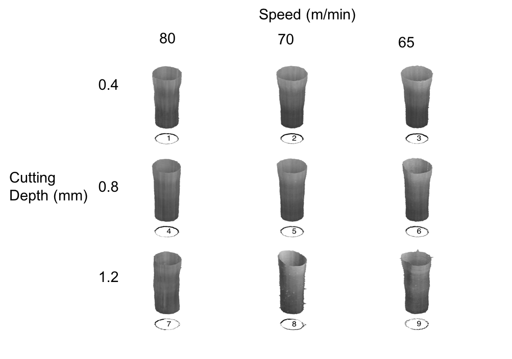
Figure 1: Examples of cylindrical surfaces in $9$ different settings. 3D colored parametric diagram (darker color refers to a minor deviation, brighter color to a major deviation). Scale 250:1

Research in the process monitoring category mainly focuses on finding unusual patterns in the point cloud to detect out-of-control states and corresponding assignable causes, e.g., combining parametric regression with univariate and multivariate control charts for quantifying 3D surfaces with spatially correlated noises. However, these models assume that a parametric model exists for 3D point clouds, which may not be true for surfaces with complex shapes. To address this challenge, Wells et al., (2013) proposed to use Q–Q plots to transform the high-dimensional point cloud monitoring into a linear profile monitoring problem. This approach, however, fails to capture the spatial information of the data as it reduces a 3D point cloud to a Q-Q plot. Colosimo et al., (2014) applied the Gaussian process to model and monitor 3D surfaces with spatial correlation. However, applying Gaussian process models can be inefficient for high-dimensional data such as those in our application. The main objective of the second category, namely, process modeling and optimization, is to build a response surface model of a structured point cloud as a function of some controllable factors. This model is then used to find the optimal control settings to minimize the dimensional and geometric deviations of produced parts from nominal values. Despite the importance of the topic, little research can be found in this area. Colosimo and Pacella, (2011) proposed a two-step approach where first a high-dimensional point cloud is reduced to a set of features using complex Principal Component Analysis (PCA) and then, the multivariate ANOVA is applied to the extracted features to test the effect of a set of scalar factors on the features mean. The main issue of the two-step approach is that the dimension reduction and modeling/test steps are carried out separately. Hence, the relationship of scalar factors with point cloud is not considered in the dimension reduction step.

Because of its grid structure, a structured point cloud can be compactly represented in a multidimensional array also known as a tensor. Therefore, modeling the structured point cloud as a function of some controllable factors can be considered as a tensor regression problem. The objective of this paper is to develop a tensor regression framework to model a tensor response as a function of some scalar predictors and use this model for prediction and process optimization. The main challenge in achieving this objective is the high dimensionality resulting in a large number of parameters to be estimated.

To achieve this, we take the advantage of the fact that the essential information of high-dimensional point cloud data lies in a low-dimensional space and we use low-dimensional basis to significantly reduce the dimensionality and the number of models parameters. To select appropriate bases, we introduce two approaches, namely One-step Tensor Decomposition Regression (OTDR) and Regularized Tensor Regression (RTR). OTDR is a data-driven approach, where the basis and coefficients are learned automatically from the tensor regression objective function. In RTR, we project the response tensor on a set of predefined basis such as Splines with roughness penalization to control the smoothness of the estimated tensor response.

The remainder of the paper is organized as follows. Section 2 gives a brief literature review on functional and tensor regression models. Section 3 provides an overview of the basic tensor notations and multilinear algebra operations. Section 4 first introduces the general regression framework for tensor response data and then elaborates the two approaches for basis selection, i.e., OTDR and RTR. Section 5 validates the proposed methodology by using simulated data with two different types of structured point clouds. In this section, the performance of the proposed method is compared with existing two-step methods in terms of the estimation accuracy and computational time. In Section 6, we illustrate a case study for process modeling and optimization in a turning process. Finally, we conclude the paper with a short discussion and an outline of future work in Section 7.

2 Literature Review

We review three categories of models in this area. The first category focuses on regression models with a multivariate vector response. For example, similar to Pacella and Colosimo, (2016), one can use a multilinear extension of PCA (Jolliffe,, 2002) to reduce the dimensionality of a multidimensional array of data (a tensor response) and then build a regression model for the estimated PC scores. Reiss et al., (2010) proposed a function-on-scalar regression, in which the functional response is linked with scalar predictors via a set of functional coefficients to be estimated in a predefined functional space. Other methods such as partial least squares (Helland,, 1990) or sparse regression Peng et al., (2010) are also capable of regressing a multivariate or functional response on scalar predictors. Although these methods are effective for modeling multivariate vectors, they are inadequate for analysis of structured point clouds due to the ultrahigh dimensionality as well as their complex tensor structures (Zhou et al.,, 2013). The second category pertains to regression models with a scalar response and tensor covariates. For example, Zhou et al., (2013) proposed a regression framework in which the dimensionality of tensor covariates is substantially reduced by applying low-rank tensor decomposition techniques leading to efficient estimation and prediction. The third category, directly related to our problem, is the modeling of a tensor response as a function of scalar predictors. (Penny et al.,, 2011) independently regressed each entry of the response tensor on scalar predictors and generated a statistical parametric map of the coefficients across the entire response tensor. This approach often required a preprocessing smoothing step to denoise the tensor response. For example, Li et al., (2011) proposed a multi-scale adaptive approach to denoise the tensor response before fitting the regression model. However, the major drawback of this approach is that all response variables are treated independently and hence, important spatial correlation is often ignored. To overcome this problem, Li and Zhang, (2016) built a parsimonious linear tensor regression model by making the generalized sparsity assumption about the tensor response. Although the sparsity assumption is valid in neuroimaging applications, it may not be valid in other point cloud applications such as the one discussed in this paper.

3 Basic Tensor Notation and Multilinear Algebra

In this section, we introduce basic notations, definitions, and operators in multilinear (tensor) algebra that we use in this paper. Throughout the paper, scalars are denoted by lowercase italic letters, e.g., $a$, vectors by lowercase boldface letters, e.g., $\mathbf{a}$, matrices by uppercase boldface letter, e.g., $\mathbf{A}$, and tensors by calligraphic letters, e.g., $\mathcal{A}$. For example, an order-$K$ tensor is represented by $\mathcal{A}\in\mathbb{R}^{I_{1}\times\cdots\times I_{K}}$, where $I_{k}$ represents the mode-$k$ dimension of $\mathcal{A}$. The mode-$k$ product of a tensor $\mathcal{A}$ by a matrix $\mathbf{V}\in\mathbb{R}^{P_{k}\times I_{k}}$ is defined by $(\mathcal{A}\times_{k}\mathbf{V})(i_{1},\cdots,i_{k-1},j_{k},i_{k+1},\cdots,i_{K})=\sum_{i_{k}}A(i_{1},\cdots,i_{k},\cdots,i_{K})V(j_{k},i_{k})$. The Frobenius norm of a tensor $\mathcal{A}$ can be defined as $\|\mathcal{A}\|_{F}^{2}=\sum_{i_{1},\cdots,i_{K}}A(i_{1},\cdots,i_{k},\cdots,i_{K})^{2}$. The n-mode unfold operator maps the tensor $\mathcal{A}$ into matrix $\mathbf{A}_{(n)}$, where the columns of $\mathbf{A}_{(n)}$ are the $n$-mode vectors of $\mathcal{A}$.

Tucker decomposition decomposes a tensor into a core tensor multiplied by a matrix along each mode, i.e., $\mathcal{A}=\mathcal{S}\times_{1}\mathbf{U}^{(1)}\times_{2}\mathbf{U}^{(2)}\cdots\times_{K}\mathbf{U}^{(K)}$, where $\mathbf{U}^{(k)}$ is an orthogonal $I_{k}\times I_{k}$ matrix and is a principal component mode-$k$. Tensor product can be represented equivalently by a Kronecker product, i.e., $\mathrm{vec}(\mathcal{A})=(\mathbf{U}^{(K)}\otimes\cdots\otimes\mathbf{U}^{(1)})\mathrm{vec}(\mathcal{S})$, where $\mathrm{vec}$ is the vectorized operator defined as $\mathrm{vec}(\mathcal{A})=\mathbf{A}_{(K+1)}$ ($\mathbf{A}_{(K+1)}$ refers to the unfolding of $\mathcal{A}$ along the additional $(K+1)^{th}$ mode, which is an $I_{1}\times I_{2}\times\cdots\times I_{K}$-dimensional vector). The definition of Kronecker product is as follow: Suppose $\mathbf{A}\in\mathbb{R}^{m\times n}$ and $\mathbf{B}\in\mathbb{R}^{p\times q}$ are matrices, the Kronecker product of these matrices, denoted by $\mathbf{A}\otimes\mathbf{B}$, is an $mp\times nq$ block matrix given by $\mathbf{A}\otimes\mathbf{B}=\left[\begin{array}[]{ccc}a_{11}\mathbf{B}&\cdots&a_{1n}\mathbf{B}\\ \vdots&\ddots&\vdots\\ a_{m1}\mathbf{B}&\cdots&a_{mn}\mathbf{B}\end{array}\right]$.

4 Tensor Regression Model with Scalar Input

In this paper, for simplicity and without loss of generality, we present our methodology with a 2D tensor response. However, this can be easily extended to higher order tensors by simply adding other dimensions. Suppose a training sample of size $N$ is available that includes tensor responses denoted by $\mathbf{Y}_{i}\in\mathbb{R}^{I_{1}\times I_{2}}$, $i=1,\cdots,N$ along with the corresponding input variables denoted by $\mathbf{x}_{i}\in\mathbb{R}^{p\times 1}$, $i=1,\cdots,N$, where $p$ is the number of regression coefficients. The tensor regression aims to link the response $\mathbf{Y}_{i}$ with the input variables $\mathbf{x}_{i}$ through a tensor coefficient $\mathcal{A}\in\mathbb{R}^{I_{1}\times I_{2}\times p}$ such that

$$\mathbf{Y}_{i}=\mathcal{A}\times_{3}\mathbf{x}_{i}+\delta\mathbf{E}_{i},i=1,\cdots,N,$$ (1)

where $\mathbf{E}_{i}$ represents the random noises. We combine the response data $\mathbf{Y}_{i}$ and the residual $\mathbf{E}_{i}$ across the samples into 3D tensors denoted by $\mathcal{Y}\in\mathbb{R}^{I_{1}\times I_{2}\times N}$ and $\mathcal{E}\in\mathbb{R}^{I_{1}\times I_{2}\times N}$, respectively. Furthermore, we combine all $\mathbf{x}_{i}$’s into a single input matrix $\mathbf{X}\in\mathbb{R^{\mathrm{\mathit{N\times p}}}}$, where the first column of $\mathbf{X}$ is $\mathbf{1}\in\mathbb{R^{\mathrm{\mathit{N\times 1}}}}$ corresponding to the intercept coefficients. Therefore, (1) can compactly be represented in the tensor format as shown in (2):

$$\mathcal{Y}=\mathcal{A}\times_{3}\mathbf{X}+\delta\mathcal{E},$$ (2)

where $\mathcal{E}$ is assumed to follow a tensor normal distribution as $\mathcal{E}\sim N(0,\Sigma_{1},\Sigma_{2},\Sigma_{3})$ (Manceur and Dutilleul,, 2013), or equivalently $e=\mathrm{vec}(\mathcal{E})\sim N(0,\Sigma_{3}\otimes\Sigma_{2}\otimes\Sigma_{1})$. $\Sigma_{1}$ and $\Sigma_{2}$ represent the spatial correlation of the noise that are assumed to be defined by $\Sigma_{k}|_{i_{1},i_{2}}=\exp(-\theta\|r_{i_{1}}-r_{i_{2}}\|^{2})=\exp(-\theta\|r_{i_{1}}-r_{i_{2}}\|^{2});k=1,2$. $\Sigma_{3}$ represents the between-sample variation. We further assume the samples are independent, and hence, $\Sigma_{3}$ is a diagonal matrix, defined by $\Sigma_{3}=diag(\sigma_{1}^{2},\sigma_{2}^{2},\cdots,\sigma_{N}^{2})$, where $diag$ is the diagonal operator that transforms a vector to a diagonal matrix with the corresponding diagonal elements. The tensor coefficients can be estimated by minimizing the negative likelihood function $\mathbf{a}$, which can be solved by $\hat{\mathcal{A}}=\mathcal{Y}\times_{3}(\mathbf{X}^{T}\Sigma_{3}^{-1}\mathbf{X})^{-1}\mathbf{X}^{T}\Sigma_{3}^{-1}$. The detailed proof is shown in Appendix A. However, since the dimensions of $\mathcal{A}$ is too high, solving $\hat{\mathcal{A}}$ directly can result in the severe overfitting. In most practical applications, however, $\mathcal{A}$ lies in a low-dimensional space. Hence, we assume that $\mathcal{A}$ can be represented in a low-dimensional space expanded by basis $\mathbf{U}^{(k)},k=1,2$, as shown in (3):

$$\mathcal{A}=\mathcal{B}\times_{1}\mathbf{U}^{(1)}\times_{2}\mathbf{U}^{(2)}+\mathcal{E}_{\mathcal{A}},$$ (3)

where $\mathcal{E}_{\mathcal{A}}$ is the residual tensor of projecting the coefficient $\mathcal{A}$ into a low-dimensional space. $\mathcal{B}\in\mathbb{R}^{P_{1}\times P_{2}\times p}$ is the core tensor (or coefficient tensor) after the projection. If $\mathbf{U}^{(k)}$ is complete, the residual tensor $\|\mathcal{E}_{\mathcal{A}}\|_{F}=0$. As $\mathcal{A}$ is low rank, we can use a set of low-dimensional bases $\mathbf{U}^{(k)}\in\mathbb{R}^{I_{k}\times P_{k}}$ (i.e., $P_{k}\ll I_{k}$) to significantly reduce the dimensionality of the coefficient tensor $\mathcal{A}$ while keeping $\|\mathcal{E}_{\mathcal{A}}\|_{F}$ close to zero. Since $\mathcal{E}_{\mathcal{A}}$ is negligible, given $\mathbf{U}^{(1)}$ and $\mathbf{U}^{(2)}$, $\mathcal{A}$ can be approximated by $\mathcal{B}\times_{1}\mathbf{U}^{(1)}\times_{2}\mathbf{U}^{(2)}$. Therefore, by combining (3) and (2), we have

$$\mathcal{Y}=\mathcal{B}\times_{1}\mathbf{U}^{(1)}\times_{2}\mathbf{U}^{(2)}\times_{3}\mathbf{X}+\delta\mathcal{E}.$$ (4)

To estimate $\mathcal{B}$, the following likelihood function can be derived, as shown in (5).

$$\min_{\mathcal{B}}l(\mathcal{B})=(\mathbf{y}-(\mathbf{X}\otimes\mathbf{U}^{(2)}\otimes\mathbf{U}^{(1)})\boldsymbol{\beta})^{T}(\Sigma_{3}\otimes\Sigma_{2}\otimes\Sigma_{1})^{-1}(\mathbf{y}-(\mathbf{X}\otimes\mathbf{U}^{(2)}\otimes\mathbf{U}^{(1)})\boldsymbol{\beta})$$ (5)

Proposition 1.

Problem (5) has a closed-form solution expressed by

$$\hat{\mathcal{B}}=\mathcal{Y}\times_{1}(\mathbf{U}^{(1)T}\Sigma_{1}^{-1}\mathbf{U}^{(1)})^{-1}\mathbf{U}^{(1)T}\Sigma_{1}^{-1}\times_{2}(\mathbf{U}^{(2)T}\Sigma_{2}^{-1}\mathbf{U}^{(2)})^{-1}\mathbf{U}^{(2)T}\Sigma_{2}^{-1}\times_{3}(\mathbf{X}^{T}\Sigma_{3}^{-1}\mathbf{X})^{-1}\mathbf{X}^{T}\Sigma_{3}^{-1}.$$ (6)

The proof of proposition 1 is shown in Appendix C.

The choice of basis $\mathbf{U}^{(k)},k=1,2$ is important to the model accuracy. In the next subsections, we propose two methods for defining basis matrices: The first method Regularized Tensor Regression (RTR) incorporates the user knowledge about the process and response; and the second method One-step Tensor Decomposition Regression (OTDR) is a one-step approach that automatically learns the basis $\mathbf{U}^{(k)},k=1,2$ and coefficients from data.

4.1 Regularized Tensor Regression (RTR) with Customized Basis Selection

In some cases, we prefer to customize the basis based on the domain knowledge and/or data characteristics. For example, a predefined spline or kernel basis can be used to represent general smooth tensors. Fourier or periodic B-spline basis can be used to represent smooth tensors with periodic boundary constraints. Furthermore, a penalty term can be added to control the level of smoothness. Consequently, the one-step regression model can be rewritten by

$$\hat{\boldsymbol{\beta}}=\mathop{\mathrm{argmin}}_{\boldsymbol{\beta}}(\mathbf{y}-(\mathbf{X}\otimes\mathbf{U}^{(2)}\otimes\mathbf{U}^{(1)})\boldsymbol{\beta})^{T}(\Sigma_{3}\otimes\Sigma_{2}\otimes\Sigma_{1})^{-1}(\mathbf{y}-(\mathbf{X}\otimes\mathbf{U}^{(2)}\otimes\mathbf{U}^{(1)})\boldsymbol{\beta})+P(\boldsymbol{\beta}).$$ (7)

However, the dimensions of $\mathbf{X}\otimes\mathbf{U}^{(2)}\otimes\mathbf{U}^{(1)}$ are $NI_{1}I_{2}\times pP_{1}P_{2}$, which is often too large to compute or even to be stored. To address this computational challenge, following (Yan et al., 2015a, ), we use a special form of the penalty term defined by

$$P(\boldsymbol{\beta})=\boldsymbol{\beta}^{T}(\mathbf{X}^{T}\Sigma_{3}^{-1}\mathbf{X})\otimes(\lambda\mathbf{P}_{2}\otimes\mathbf{U}^{(1)^{T}}\Sigma_{1}^{-1}\mathbf{U}^{(1)}+\lambda\mathbf{U}^{(2)^{T}}\Sigma_{2}^{-1}\mathbf{U}^{(2)}\otimes\mathbf{P}_{1}+\lambda^{2}\mathbf{P}_{2}\otimes\mathbf{P}_{1})\boldsymbol{\beta},$$ (8)

where $\boldsymbol{\beta}=\mathrm{vec}(\mathcal{B})$, $\mathbf{P}_{k}=(\mathbf{D}_{k}^{2})^{T}\mathbf{D}_{k}^{2}$ is the penalization matrix to control the smoothness among the mode-$k$ of the original tensor. As shown in (Xiao et al.,, 2013) and (Yan et al., 2015a, ), the penalty term defined with tensor structure works well in the simulation and achieve the optimal rate of convergence asymptotically under some mild conditions. In Proposition 2 We prove that by using this $P(\mathcal{B})$, not only does Problem (7) have a closed-form solution, but also the solution can be computed along each mode of the original tensor separately, which significantly reduces the computational complexity.

Proposition 2.

The optimization problem (7) with $P(\mathcal{B})$ defined in (8) can efficiently be solved via a tensor product given by

$$\hat{\mathcal{B}}=\mathcal{Y}\times_{1}(\mathbf{U}^{(1)^{T}}\Sigma_{1}^{-1}\mathbf{U}^{(1)}+\lambda\mathbf{P}_{1})^{-1}\mathbf{U}^{(1)^{T}}\Sigma_{1}^{-1}\times_{2}(\mathbf{U}^{(2)^{T}}\Sigma_{2}^{-1}\mathbf{U}^{(2)}+\lambda\mathbf{P}_{2})^{-1}\mathbf{U}^{(2)^{T}}\Sigma_{2}^{-1}\times_{3}(\mathbf{X}^{T}\Sigma_{3}^{-1}\mathbf{X})^{-1}\mathbf{X}^{T}\Sigma_{3}^{-1}.$$ (9)

The proof is given in Appendix D. The tuning parameter selection will be discussed in section 4.3.

Assuming $I_{1}=I_{2}=I_{0}$, the computational complexity of the RTR method in each iteration is $O(I_{0}^{2}N^{2}p)$ provided that the covariance matrix is computed beforehand to save the computational time in each iteration.

4.2 One-step Tensor Decomposition Regression (OTDR)

In cases where little engineering or domain knowledge is available, it is necessary to learn the basis from the data. Similar to principal component regression, one technique is to learn the basis from Tucker decomposition and apply the regression on the Tucker decomposition core tensor. The details of this method is given in Appendix B. However, the major limitation of this two-step approach is that the learned basis may not correspond to the input variables $\mathbf{X}$.

Consequently, in this section, we propose a one-step approach to learn the basis and coefficients at the same time. To achieve this, we propose to simultaneously optimize both the coefficient $\boldsymbol{\beta}$ and basis $\mathbf{U}^{(k)}$ in 5. Moreover, instead of the orthogonality constraint on $\mathbf{U}^{(i)},i=1,2$ , we apply the weighted constraint given by $\mathbf{U}^{(k)T}\Sigma_{i}^{-1}\mathbf{U}^{(k)}=I$. This constraint not only results in a closed-form solution in each iteration, but also ensures that the estimated basis and residuals share a similar spatial covariance structure.

$$\mathop{\mathrm{argmin}}_{\boldsymbol{\beta},\mathbf{U}^{(k)}}(\mathbf{y}-(\mathbf{X}\otimes\mathbf{U}^{(2)}\otimes\mathbf{U}^{(1)})\boldsymbol{\beta})^{T}(\Sigma_{3}\otimes\Sigma_{2}\otimes\Sigma_{1})^{-1}(\mathbf{y}-(\mathbf{X}\otimes\mathbf{U}^{(2)}\otimes\mathbf{U}^{(1)})\boldsymbol{\beta})$$

$$s.t.\quad\mathbf{U}^{(k)T}\Sigma_{k}^{-1}\mathbf{U}^{(k)}=I$$ (10)

To efficiently optimize (10), we use the alternative least square approach, which optimizes $\mathcal{B}$, $\mathbf{U}^{(1)}$, $\mathbf{U}^{(2)}$, iteratively. From proposition (1), we know that if $\mathbf{U}^{(k)},k=1,2$ are given, $\mathcal{B}$ has a closed-form solution as the one in (5). To optimize $\mathbf{U}^{(k)},k=1,2$, we use the following proposition.

Proposition 3.

Minimizing the negative log-likelihood function in (5) is equivalent to maximizing the projected scores norm in (11),

$$\arg\max_{\mathbf{U^{(k)}}}\|\mathcal{Y}\times_{1}\mathbf{U}^{(1)^{T}}\Sigma_{1}^{-1}\times_{2}\mathbf{U}^{(2)^{T}}\Sigma_{2}^{-1}\times_{3}\mathbf{X}_{3}\|^{2};k=1,2,$$

$$s.t.\quad\mathbf{U}^{(k)T}\Sigma_{k}^{-1}\mathbf{U}^{(k)}=I,$$ (11)

where $\mathbf{X}_{3}$ can be computed by the Cholesky decomposition as $\mathbf{X}_{3}\mathbf{X}_{3}^{T}=\Sigma_{3}^{-1}\mathbf{X}(\mathbf{X}^{T}\Sigma_{3}^{-1}\mathbf{X})^{-1}\mathbf{X}^{T}\Sigma_{3}^{-1}$. Furthermore, given $\mathbf{U}^{(i)}$, the maximizer of (11) is given by $\mathbf{U}^{(k)}=\Sigma_{k}^{1/2}\mathbf{\tilde{U}}^{(k)},$ where $\mathbf{\tilde{U}}^{(k)}$ is the first $P_{k}$ eigenvectors of $\Sigma_{k}^{-1/2}\mathbf{W}_{k}$. $\mathbf{W}_{k}$ is the $k^{th}$ mode unfolding of $\mathcal{W}_{k}=\mathcal{Y}\times_{3-k}\mathbf{U}^{(i)}\Sigma_{3-k}^{-1}\times_{3}\mathbf{X}_{3}$.

The procedure for performing OTDR is given in Algorithm 1. The fact that the resulting sub-problem in each iteration reduces to a generalized eigenvalue problem significantly speeds up the algorithm. Thus, assuming that $P_{1}=P_{2}=P_{0}$ and $I_{1}=I_{2}=I_{0}$, the complexity of the algorithm in each iteration is $O(\min(P_{0}^{2}NI_{0},N^{2}I_{0}^{2}P_{0}))$, provided that $\Sigma_{k}^{-1},\Sigma_{k}^{1/2},\Sigma_{k}^{-1/2}$ is computed beforehand.

Similar to many non-convex models such as Tucker decomposition and matrix factorization (Kolda and Bader,, 2009), the solution of OTDR is not unique. For example, it is possible to define an orthogonal transformation $\mathbf{R}_{k}$ on the basis $\mathbf{U}^{(k)}$ as $\mathbf{U}_{1}^{(k)}=\mathbf{U}^{(k)}\mathbf{R}_{k}$, and $\beta_{1}=(I\otimes\mathbf{R}_{2}^{-1}\otimes\mathbf{R}_{1}^{-1})\beta$ such that the fitted response $\hat{\mathbf{y}}=(\mathbf{X}\otimes\mathbf{U}^{(2)}\otimes\mathbf{U}^{(1)})\boldsymbol{\beta}$ stays the same and the constraint still holds. However, different matrix factorization and tensor decomposition models are still widely used despite the non-uniqueness of the solution (Kolda and Bader,, 2009). The reason is that over-complete representation is more flexible and robust to noise and the fitted response will not be affected (Anandkumar et al.,, 2013). However, if uniqueness of parameter is important, it is possible to add the sparsity constraint on the core tensor so that the algorithm will search for the rotation to make as many elements $0$ as possible (Anandkumar et al.,, 2013). For more detailed discussions about the over-complete representation in the application of tensor decomposition, please refer to (Anandkumar et al.,, 2013).

• Initialize

  Compute $\Sigma_{k}^{-1},\Sigma_{k}^{1/2},\Sigma_{k}^{-1/2}$ and compute $X_{3}$ through the Cholesky decomposition as $\mathbf{X}_{3}\mathbf{X}_{3}^{T}=\Sigma_{3}^{-1}\mathbf{X}(\mathbf{X}^{T}\Sigma_{3}^{-1}\mathbf{X})^{-1}\mathbf{X}^{T}\Sigma_{3}^{-1}$

• For $i=1,2,\cdots$, $k=1,2$

  Compute $\mathcal{W}_{k}=\mathcal{Y}\times_{3-k}\mathbf{U}^{(3-k)^{T}}\Sigma_{3-k}^{-1}\times_{3}X_{3}$,

  Compute $\mathbf{W}_{k}$ as the $k$-th mode unfolding of $\mathcal{W}_{k}$.

  Compute $\mathbf{\tilde{U}}^{(k)}$ is the first $P_{k}$ eigenvectors of $\Sigma_{k}^{-1/2}\mathbf{W}_{k}$,

  Update$\mathbf{U}^{(k)}=\Sigma_{k}^{1/2}\mathbf{\tilde{U}}^{(k)}$ until convergence

• Compute $\mathcal{B}$ based on (6)

Algorithm 1 ALS algorithm for RTD

4.3 Tuning Parameter Selection

In this section, we propose a procedure for selecting the tuning parameters including the smoothness parameter $\lambda$ in RTD and RTR, and the covariance parameter $\theta$ in OTDR. To select tuning parameter $\lambda$ in RTR, since the formulation follows the standard ridge regression format, the Generalized Cross Validation (GCV) criterion can be used. That is, $\hat{\lambda}=\arg\min_{\lambda}\mathrm{GCV}(\lambda)=\arg\min_{\lambda}\frac{\|\mathcal{Y}-\hat{\mathcal{B}}\times_{1}\mathbf{U}^{(1)}\times_{2}\mathbf{U}^{(2)}\times_{3}\mathbf{X}\|^{2}/N}{(1-N^{-1}\mathrm{tr}(\hat{\mathbf{H}}_{1}(\lambda))\mathrm{tr}(\hat{\mathbf{H}}_{2}(\lambda))\mathrm{tr}(\hat{\mathbf{H}}_{3}(\lambda)))^{2}}$, where $\hat{\mathbf{H}}_{k}(\lambda)=\mathbf{U}^{(k)}(\mathbf{U}^{(k)^{T}}\mathbf{U}^{(k)}+\lambda\mathbf{P}_{k})^{-1}\mathbf{U}^{(k)^{T}}$, $k=1,2$, and $\hat{\mathbf{H}}_{3}(\lambda)=\mathbf{X}(\mathbf{X}^{T}\mathbf{X})^{-1}\mathbf{X}^{T}$.

In the OTDR model, we propose to find the set of tuning parameters including the covariance parameters $\theta$, $\sigma$, and number of PCs $P_{1}$, $P_{2}$ by minimizing the BIC criterion defined in (12), where $P_{1}$ and $P_{2}$ are number of bases in $\mathbf{U}^{(1)}$ and $\mathbf{U}^{(2)}$.

$$\min_{\theta,\sigma,P_{1},P_{2}}BIC=N\ln(\frac{1}{N}(\mathbf{y}-(\mathbf{X}\otimes\mathbf{U}^{(2)}\otimes\mathbf{U}^{(1)})\boldsymbol{\beta})^{T}(\Sigma_{3}\otimes\Sigma_{2}\otimes\Sigma_{1})^{-1}(\mathbf{y}-(\mathbf{X}\otimes\mathbf{U}^{(2)}\otimes\mathbf{U}^{(1)})\boldsymbol{\beta})+(P_{1}+P_{2})p\ln N$$ (12)

5 Simulation Study

In this section, we conduct simulations to evaluate the performance of the proposed OTDR and RTR for structured point cloud modeling. We simulate $N$ structured point clouds as training samples $\mathbf{Y}_{i},i=1,\cdots,N$ for two different responses, namely, a wave-shape response surface and a truncated cone response. The simulated data is generated according to $\mathbf{Y}_{i}=\mathbf{M}+\mathbf{V}_{i}+\mathbf{E}_{i}$, or equivalently in the tensor form, $\mathcal{Y}=\mathcal{M}+\mathcal{V}+\mathcal{E}$, where $\mathcal{Y}$ is a 3rd order tensor combining $\mathbf{Y}_{i},i=1,\cdots,N$, $\mathcal{M}$ is the mean of the point cloud data and $\mathcal{V}$ is the variational pattern of the point cloud due to different levels of input variables, $\mathbf{x}_{i}$. $\mathcal{E}$ is a tensor of random noises. We consider two cases to generate noises: 1) i.i.d noise, where $\mathbf{E}_{i}\overset{i.i.d}{\sim}N(0,\sigma^{2})$; and 2) non-i.i.d noise, $e=\mathrm{vec}(\mathcal{E})\sim N(0,\Sigma_{3}\otimes\Sigma_{2}\otimes\Sigma_{1})$. Since the point cloud is spatially correlated, we put the spatial correlation structure on the covariance matrix on two spatial axes $\Sigma_{1},\Sigma_{2}$, i.e., $\Sigma_{1}|_{i_{1},i_{2}}=\Sigma_{2}|_{i_{1},i_{2}}=\exp(-\theta\|r_{i_{1}}-r_{i_{2}}\|^{2})$.

Case 1. Wave-shape surface point cloud simulation

We simulate the surface point cloud in a 3D Cartesian coordinate system $(x,y,z)$ where $0\leq x,y\leq 1$. The corresponding $z_{i_{1}i_{2}}$ values at $(\frac{i_{1}}{I_{1}},\frac{i_{2}}{I_{2}}),i_{1}=1,\cdots,I_{1};i_{2}=1,\cdots I_{2}$, with $I_{1}=I_{2}=200$ for $i^{th}$ sample recorded in the matrix $\mathbf{Y}_{i}$, is generated by $\mathcal{Y}=\mathcal{V}+\mathcal{E}$. We simulate the variational patterns of point cloud surface $\mathcal{V}$, according to the following linear model $\mathcal{V}=\mathcal{B}\times_{1}\mathbf{U}^{(1)}\times_{2}\mathbf{U}^{(2)}\times_{3}\mathbf{X}$. In the simulation setup, we select three basis matrices, namely $\mathbf{U}^{(k)}=[\mathbf{u}_{1}^{(k)},\mathbf{u}_{2}^{(k)},\mathbf{u}_{3}^{(k)}]$ with $\mathbf{u}_{\alpha}^{(k)}=[\sin(\frac{\pi\alpha}{n}),\sin(\frac{2\pi\alpha}{n}),\cdots,\sin(\frac{n\pi\alpha}{n})]^{T},\alpha=1,2,3$. The two mode-3 slices of $\mathcal{B}\in\mathbb{R}^{3\times 3\times 2}$ is generated as $\mathbf{B}_{1}=\left[\begin{array}[]{ccc}4&1&0\\ 1&0.1&0\\ 1&0&1\end{array}\right]$, $\mathbf{B}_{2}=\left[\begin{array}[]{ccc}1&2&0\\ 1&3&0\\ 1&0&0.2\end{array}\right]$. The input matrix $\mathbf{X}$ are randomly sampled from the standard normal distribution $N(0,1)$. In this study, we generate 100 samples according the foregoing procedure. The examples of the generated point cloud surface with the i.i.d noise and non-i.i.d noise ($\theta=10$) are shown in Figure 2.

Case 2. Truncated cone point cloud simulation

We simulate truncated cone point clouds in a 3D cylindrical coordinate system $(r,\phi,z)$, where $\phi\in[0,2\pi]$, $z\in[0,1]$. The corresponding $r$ values at $(\phi,z)=(\frac{2\pi i_{1}}{I_{1}},\frac{i_{2}}{I_{2}})$, $i_{1}=1,\cdots,I_{1};i_{2}=1,\cdots I_{2}$ with $I_{1}=I_{2}=200$ for the $i^{th}$ sample are recorded in the matrix $\mathbf{Y}_{i}$. We simulate the variational patterns of point cloud surface $\mathcal{V}$ according to $r(\phi,z)=\frac{r+z\tan\theta}{\sqrt{1-e^{2}\cos^{2}\phi}}+c(z^{2}-z)$ with three different settings ($0.9\times$, $1\times$, and $1.1\times$) of the normal setting, i.e., $\theta_{0}=\frac{\pi}{8},r_{0}=1.3,e_{0}=0.3,c_{0}=0.5$ , which corresponds to 1) different angles of the cone; 2) different radii of the upper circle; 3) different eccentricities of top and bottom surfaces; and 4) different curvatures of the side of the truncated cone. Furthermore, we define four input variables by $x_{1}=\tan\theta$, $x_{2}=r$, $x_{3}=e^{2}$, $x_{4}=c$ and record them in an input matrix $\mathbf{X}$ of size $81\times 4$. These nonlinear transformations lead to a better linear approximation of the point cloud in the cylindrical coordinate system given the input matrix $\mathbf{X}$. Finally, we use a full factorial design to generate $3^{4}=81$ training samples with different combinations of the coefficients. The examples of the generated truncated cones with i.i.d noise and non-i.i.d noise ($\theta=10$) are shown in Figure 2. We simulated 1000 test examples $\mathcal{Y}_{te}$ based on different settings of $\theta,r,e,c$ (uniformly between the lowest and highest settings in the design table).

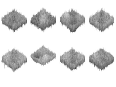
(a) Case 1 with i.i.d noise

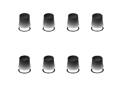
(b) Case 2 with i.i.d noise

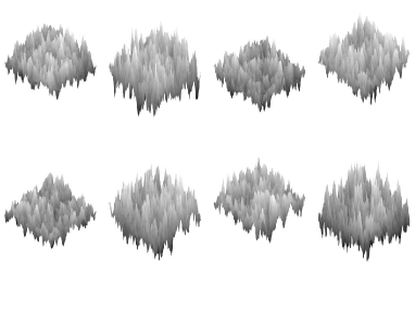
(c) Case 1 with non-i.i.d noise

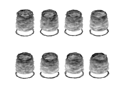
(d) Case 2 with non-i.i.d noise

Figure 2: Examples of generated point cloud for simulation study with i.i.d and non i.i.d noise

For both cases, the goal is to find the relationship between the point cloud tensor $\mathcal{Y}$ and input variables $\mathbf{X}$. We compare our proposed RTR and OTDR with two existing methods in the literature. The benchmark methods we used for comparison include vectorized principal component analysis regression (VPCR), Tucker decomposition regression (TDR) and simple linear regression (LR). For VPCR, PCA is applied on the unfolded matrix denoted by $\mathbf{Y}_{(3)}$. In LR, we separately conduct a linear regression for each entry of the tensor $\mathcal{Y}$ with the input variables $\mathbf{X}$. In TDR, we use basis matrices learned from Tucker Decomposition of the data. For RTR, we use B-spline with 20 knots on each dimension. It should be noted that in Case 2, we apply the periodic B-spline with the period of $2\pi$ to model the periodicity in the $\theta$ direction. In OTDR, the basis is automatically learned from the data. The tuning parameters of RTR and OTDR are selected by using the GCV and BIC criteria. For Case 1 and 2, the relative sum of squared error (SSE) between $\mathcal{Y}_{te}$ and the predicted tensor $\hat{\mathcal{Y}}_{te}$ defined by $\frac{\|\mathcal{Y}_{te}-\hat{\mathcal{Y}}_{te}\|^{2}}{\|\hat{\mathcal{Y}}_{te}-\bar{\mathcal{Y}}_{te}\|^{2}}$ is computed from 10,000 simulation replications under different noise levels, $\delta$, and two noise structures: i.i.d and non-i.i.d with different $\theta$ values. The results are reported in Tables 1. Furthermore, the average computational time per sample for each method is reported: RTR, 1.19s; OTDR, 1.7s; VPCR, 0.97s; and LR, 0.77s. It can be seen that the proposed RTR and OTDR have a similar level of complexity to VPCR. Recall that the complexities of RTR, OTDR, and VPCR are $O(I_{0}^{2}N^{2}p)$, $O(\min(P_{0}^{2}NI_{0},N^{2}I_{0}^{2}P_{0}))$, and $O(I_{0}^{2}N^{2})$ respectively. As $p$ and $P_{0}$ are often small, the complexity of these methods are roughly the same.

Table 1: SSEs (Unit: percentage %) of the proposed methods when $\sigma=1$ with i.i.d and non-i.i.d noise ($\theta=10$)

	Case 1				Case 2
	Non i.i.d		i.i.d		Non i.i.d		i.i.d
$\delta=0.1$	Mean	STD	Mean	STD	Mean	STD	Mean	STD
RTR	136.79	6.69	0.36	0.00048	2.91	0.24	0.0012	4.e-06
TDR	57.44	29.96	0.00043	1e-05	3.08	0.71	9e-05	4e-07
VPCR	60.72	27.39	0.028	9e-05	2.87	0.78	0.0016	3e-06
LR	50.37	29.36	0.028	9e-05	3.19	0.69	0.0018	5e-06
OTDR	22.88	8.79	0.00043	1e-05	0.23	0.28	9e-05	4e-07
$\delta=1$	Mean	STD	Mean	STD	Mean	STD	Mean	STD
RTR	110.38	34.57	0.36	0.0058	1.85	1.03	0.0012	6e-05
TDR	552.14	195.08	0.04	0.002	36.69	5.99	0.0013	7e-05
VPCR	422.57	188.02	2.79	0.009	29.49	7.98	0.092	0.0027
LR	947.11	202.33	2.78	0.0091	56.93	8.23	0.18	0.00061
OTDR	311.19	120.51	0.04	0.002	7.64	4.00	0.0015	0.0001

From Table 1, we can conclude that the proposed OTDR outperforms all other methods when the noise level is small and is only second to RTR when the noise level is large. This superiority is due to two reasons: 1) OTDR can utilize the tensor structure of point cloud data, while RTR can capture its smoothness; and 2) OTDR can simultaneously perform dimension reduction and learn regression coefficients. To understand the the contribution of each component (i.e., one-step approach, smoothness, and the tensor structure) in improving the model accuracy, we take a closer look at simulation results: a) Benefit of the one-step approach for non-i.i.d noises: In Case 2 with $\delta=1$, the relative SSE of TDR is $36.69\%$ compared to $7.64\%$ of OTDR. This indicates that the advantage of the one-step approach (OTDR) over the two-step approach (TDR) becomes more pronounced for highly correlated noises. On the other hand, if the noise is i.i.d, the relative SSE of the OTDR and TDR are very similar. The reason is that for i.i.d. noises, most of the variational patterns learned through PCs, directly correlate with the input variables $X$, not with the noise structure; b) Benefit of utilizing the tensor structure: We compare the performance of TDR and VPCR, which are two-step approaches. They both first reduce the dimensions of the point clouds, and then, perform regression on the low-dimensional features. However, unlike VPCR, TDR utilizes the tensor structure of the data. If $\theta$ is large, the relative SSE of TDR is much smaller than that of VPCR, especially when the noise level $\delta$ is large. For example, for i.i.d noises, the relative SSE is $0.0013$% for TDR compared to $0.092\%$ for VPCR when $\delta=1$; c) Benefit of capturing smoothness : The proposed RTR outperforms other methods when $\delta$ is large. For example, in Case 1, for non i.i.d case and $\delta=1$, the relative SSE of RTR is $1.85\%$, much smaller than that of the second best, OTDR, which is $7.64\%$.

We then plot the learned coefficient $\mathcal{A}$ for VPCR, OTDR and RTR for Case 1 and 2 in Figure 3 and 4, respectively. From these plots, we can see that RTR learns a much smoother coefficient due to the use of smooth basis. However, this constraint may lead to a larger bias when the noise level is small for non-i.i.d noises (See Figure 3 (d) as an example). Furthermore, although OTDR does not incorporate any prior smoothness, the learned basis matrices are much smoother than those of VPCR. This can be seen clearly by comparing Figure 3 (b), (f) with (d), (h); and by comparing Figure 4 (b), (f) with (d), (h). This is because OTDR utilizes the tensor structure. Furthermore, in the non i.i.d noise case, all the methods perform worse than in the case with the i.i.d noise. However, the one-step approach OTDR still learns more accurate basis than TDR. This can be seen clearly seen by comparing Figure 4 (g) with (h) and by comparing Figure 3 (g) with (h).

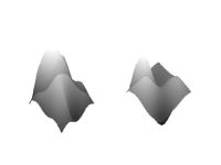
(a) RTR

(b) OTDR

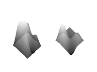
(c) TDR

(d) VPCR

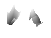
(e) RTR

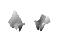
(f) OTDR

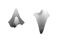
(g) TDR

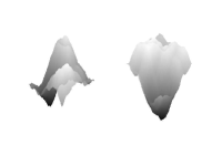
(h) VPCR

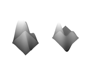
(i) True coefficient

Figure 3: Estimated and true coefficient for Case 1 with $\delta=0.1$ (1st row: i.i.d noise; 2nd row non-i.i.d noise with $\theta=10$)

(a) RTR

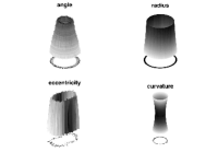
(b) OTDR

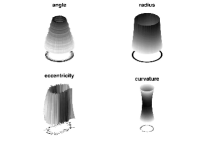
(c) TDR

(d) VPCR

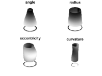
(e) RTR

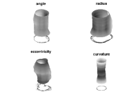
(f) OTDR

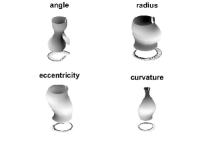
(g) TDR

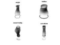
(h) VPCR

Figure 4: Estimated and true coefficient for Case 2 with $\delta=0.1$ (1st row: i.i.d noise; 2nd row non-i.i.d noise with $\theta=10$)

6 Case Study

In this section, a real case study concerning cylindrical surfaces obtained by lathe-turning is described and taken as reference in order to analyze the proposed methods. The study refers to cylinders of material Ti-6Al-4V, which is a titanium alloy principally used in the aerospace field because of certain properties (e.g., high specific strength, corrosion and erosion resistance, high fatigue strength) that make it the ideal structural material of mechanical components for both airframes and engines (Peters et al.,, 2003). While aerospace applications require significant machining of mechanical components, titanium and its alloys are generally classified as difficult-to-machine materials (Pramanik,, 2014; Pervaiz et al.,, 2014). Combinations of machining parameters, such as the cutting speed, cutting depth and feed rate, are varied and optimized in order to improve machinability and thereby improving part quality.

6.1 The Reference Experiment

Various investigations have been conducted in the literature to achieve the most favorable cutting conditions of titanium alloys by optimizing the process parameters (Khanna and Davim,, 2015; Chauhan and Dass,, 2012). In this paper, the experiment described in (Pacella and Colosimo,, 2016) is considered as reference. Bars supplied in $20$mm diameter, were machined to a final diameter of $16.8$mm by implementing two cutting steps. During the experiment, the combinations of two parameter values were varied according to a $3^{2}$ full factorial design. In particular, with reference to the second cutting step, the cutting speed was set at $65$, $70$ and $80$ m/min, while cutting depth was set at $0.4$, $0.8$ and $1.2$ mm. The combinations of parameters used are shown in Table 2, which shows $9$ treatments with different process variables (each treatment replicated $10$ times). In order to apply the proposed methods to the experimental data, the two process variables (cutting depth and cutting speed) were recorded in the input matrix $\mathbf{X}$ after the normalization (subtract the mean and divided by the standard deviation).

Table 2: Cutting parameters for $9$ experimental conditions

Ex. No	Depth($mm$)	Speed($m/min$)
1	0.4	80
2	0.4	70
3	0.4	65
4	0.8	80
5	0.8	70
6	0.8	65
7	1.2	80
8	1.2	70
9	1.2	65

The $90$ cylindrical surfaces were measured with a CMM using a touch trigger probe with a tip stylus of $0.5$ mm radius. The measurements were taken in $42$ mm along the bar length direction with $210$ cross-sections. Each cross-section was measured with $64$ generatrices. A set of $210\times 64$ points, equally distributed on the cylindrical surface, was measured for each sample $\mathbf{Y}_{i},i=1,\cdots,90$. All the samples were aligned by rotation (Silverman,, 1995). The final surface data was computed as deviations of the measured radii from a reference cylinder, which was computed using a least-square approach. By subtracting the radius of the substitute geometry, the final set of measurements consists of a set of radial deviations from a perfect cylinder, measured at each position.

The examples of the cylindrical surfaces are shown in Figure 1, which clearly shows that the shape of the cylinder is influenced by both the cutting speed and cutting depth. In particular, a taper axial form error (Henke et al.,, 1999) is the most evident form error for cylindrical surfaces. This was mainly due to deflection of the workpiece during turning operations. The degree of the deflection at cutting location varies and depends on how far the cutting tool is from the supporters of the chuck (Zhang et al.,, 2005).

6.2 Surface Roughness

While surface shape represents the overall geometry of the area of interest, surface roughness is a measurement of the surface finish at a lower scale (surface texture). Surface roughness is commonly characterized with a quantitative calculation, expressed as a single numeric parameter of the roughness surface, which is obtained from a high-pass filtering of the measured surface after the shortest wavelength components are removed. In the reference case study, the measured surface is obtained from scanning the actual surface with a probe which mechanically filters this data due to the CMM tip radius (0.5 mm). Given the CMM measurements in the experiments, the variance of residuals after modeling the shape of cylindrical items is assumed as the quantitative parameter related to surface roughness.

In machining the titanium alloy, several surface roughness prediction models - in terms of the cutting speed, feed rate and cutting depth - have been reported in the literature (e.g., Ramesh et al., (2012)). In general, it has been found that cutting depth is the most significant machining parameter. In the experiment of (Pacella and Colosimo,, 2016) an unequal residual variance, caused by different process variables, was observed.

6.3 Handling Unequal Variances of Residuals

In order to model both the cylindrical mean shape and the residuals with unequal variance (unequal surface roughness) caused by the different process variables, we combine the framework proposed by (Western and Bloome,, 2009) with our proposed tensor regression model in Section 6.3.

To model the unequal variances of residuals as a function of the process variables, we assume that the noise $E_{i}\sim N(0,\sigma_{i}^{2})$, where $\log\sigma_{i}^{2}=\mathbf{x}_{i}^{\prime}\boldsymbol{\gamma}+\gamma_{0}$. Therefore, by combining it with the tensor regression model in (1), the maximum likelihood estimation (MLE) method can be used to estimate the parameters $\boldsymbol{\gamma}$, $\gamma_{0}$ and $\mathcal{A}$. The likelihood function (for the i.i.d noise) is given by $L(\beta,\boldsymbol{\gamma};y_{i})=-\frac{1}{2}(\sum_{i}I_{1}I_{2}\log(\sigma_{i}^{2})+\sum_{i}\frac{\|\mathbf{Y}_{i}-\bar{\mathbf{Y}}-\mathcal{A}\times_{3}\mathbf{X}_{i}\|^{2}}{\sigma_{i}^{2}})$, which can be maximized by iteratively updating $\boldsymbol{\gamma}$ and $\mathcal{A}$ until convergence according to the following procedure: 1) For the fixed $\boldsymbol{\gamma}$ and $\gamma_{0}$, perform transformations given by $\mathbf{Y}_{i}^{0}=\frac{\mathbf{Y}_{i}-\bar{\mathbf{Y}}}{\sigma_{i}}$, $\mathbf{X}_{i}^{0}=\frac{\mathbf{X}_{i}}{\sigma_{i}}$, where $\sigma_{i}^{2}=\exp(\mathbf{x}_{i}^{\prime}\boldsymbol{\gamma}+\gamma_{0})$. The resulting MLE can be obtained by the proposed tensor regression methods introduced in Section (4). 2) For fixed $\mathcal{A}$, MLE reduces to gamma regression with $\log$ link on the Residual Mean Squares Error (RMSE), i.e., $\frac{1}{I_{1}I_{2}}\|\hat{\mathbf{E}}_{i}\|^{2}$, where $\hat{\mathbf{E}}_{i}=\mathbf{Y}_{i}-\mathcal{A}\times_{3}\mathbf{X}_{i}$.

We then apply OTDR on these cylindrical surfaces to map the relationship of the mean shape and residual variance with process variables. The first nine ($3\times 3$) eigentensors of OTDR are extracted and shown in Figure 5.

From Figure 5, it can be observed that the shape of eigentensors can be interpreted as the combination of both bi-lobed and three-lobed contours along the radial direction, to conical shapes along the axial direction. This result is consistent with that reported in the literature where a conical shape along the vertical (referred to as taper error) was defined as a “dominant” axial form error of manufactured cylindrical surfaces. Similarly, radial form errors are often described as bi-lobed (oval) and three-lobed (three-cornered) contours, which are typical harmonics that characterize the cross-section profiles of cylinders obtained by lathe-turning (Henke et al.,, 1999). The estimated coefficients, $\hat{\mathcal{A}}$, are also shown in Figure 6a. A visual inspection of this figure shows that the systematic shape characterizing the tensor regression coefficients relates to the cutting depth and speed parameters, i.e., a conical shape whose inferior portion assumes a bi-lobed contour. Again, the result is consistent with that reported in the literature where a conical shape is a common axial form error of manufactured cylindrical surfaces, and a bi-lobed contour is a typical harmonic that characterize the cross-section profiles of cylinders obtained by lathe-turning (Henke et al.,, 1999).

The RMSE and the fitted $\sigma^{2}$ of the $90$ samples via the gamma regression are shown in Figure 6b. It is clear that the proposed framework is able to account for unequal variances under the $9$ different input settings. The gamma regression coefficients of the RMSE are reported in Table 3. From this table, we can conclude that if the cutting depth increases or cutting speed decreases, the variance of residuals will also increase. Moreover, for the variance of residuals (surface roughness), the effect of the cutting depth is much more significant than the that of the cutting speed. These findings are consistent with engineering principles.

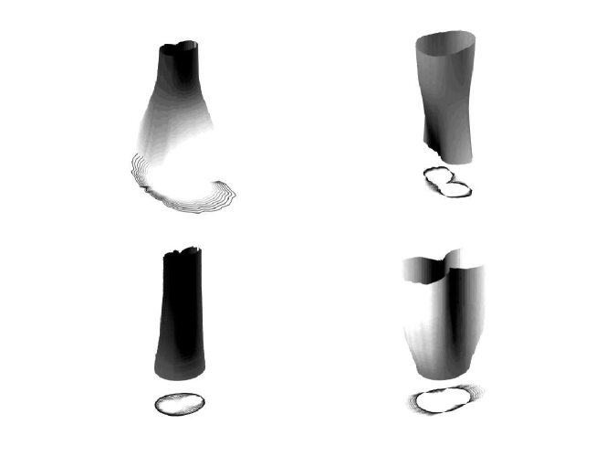
Figure 5: Eigentensors learned from OTDR with regularized Tucker decomposition

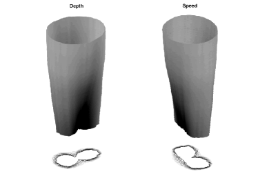
(a) Tensor regression coefficient $\mathcal{A}$

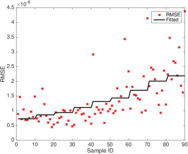
(b) Residual Mean of Square Error (RMSE) and fitted $\hat{\sigma}^{2}$ via gamma regression

Figure 6: Result of tensor regression via OTDR

Table 3: Gamma regression of $\|\hat{E}_{i}\|^{2}$

		Estimate	SE	t-Stat	p-Value
$\gamma_{0}$	Intercept	$-13.5681$	$0.0455$	$-298.12$	$1e-133$
$\boldsymbol{\gamma}$	depth	$0.3654$	$0.0483$	$7.568$	$3.7e-11$
	speed	$-0.1121$	$0.0483$	$-2.322$	$0.02$

6.4 Process Optimization

The estimated tensor regression model can also provide useful information to optimize the process settings (cutting depth and cutting speed) for better product quality. In this turning process, the goal is to produce a cylindrical surface with a uniform radius $r_{t}=16.8\mathrm{mm}$. Therefore, the objective function is defined as the sum of squared differences of the produced mean shape and the uniform cylinder with radius $r_{t}$. Furthermore, we require the produced variance of residuals, $\sigma$ , to be smaller than a certain threshold, $\sigma_{0}$. Finally, the process variables are typically constrained in a certain range defined by $\mathbf{l}\leq\mathbf{x}\leq\mathbf{u}$ due to the physical constraints of the machine. Therefore, the following convex optimization model can be used for optimizing the turning process:

$$\min_{\mathbf{x}}\|\bar{\mathbf{Y}}+\hat{\mathcal{A}}\times_{3}\mathbf{x}-r_{t}\|_{F}^{2}\quad s.t.\sigma\leq\sigma_{0},\mathbf{l}\leq\mathbf{x}\leq\mathbf{u}.$$

It is straightforward to show that this optimization problem can be reformulated to a quadratic programming (QP) model with linear constraints as

$$\min_{\mathbf{x}}\mathbf{x}^{T}\mathbf{A}_{(3)}^{T}\mathbf{A}_{(3)}\mathbf{x}+2\mathbf{x}^{T}\mathbf{A}_{(3)}^{T}(\mathrm{vec}(\bar{\mathbf{Y}})-r_{t})\quad s.t.\boldsymbol{\gamma}^{\prime}\mathbf{x}\leq\log(\sigma_{0}^{2})-\gamma_{0},\mathbf{l}\leq\mathbf{x}\leq\mathbf{u}.$$

Since the problem is convex, it can be solved via a standard quadratic programming solver. For example, if $\sigma_{0}=0.0001$ and process variables are limited to the range defined by the design matrix in Table 2, the optimal cutting speed and cutting depth are computed as $80\mathrm{m/min}$ and $0.7264\mathrm{mm}$, respectively. Under this setting, we simulate the produced cylindrical surfaces as shown in Figure 7b by combining both the predicted surface $\hat{\mathbf{Y}}=\bar{\mathbf{Y}}+\hat{\mathcal{A}}\times_{3}\mathbf{x}$ and generated noises from the normal distribution with the estimated standard deviation by $\hat{\sigma}=\exp(\frac{1}{2}(\gamma_{0}+\boldsymbol{\boldsymbol{\gamma}}^{\prime}\hat{\mathbf{x}}))$. It is clear that the produced cylindrical surfaces under this optimal setting is closer to the uniform cylinder compared than other input settings as shown in Figure 1. To show the optimal setting for different levels of the $\sigma_{0}$, we plot the relationship between the optimal cutting depth and the right hand side of the roughness constraint, $\sigma_{0}$ in Figure 7a. It is worth noting that for all $\sigma_{0}$ larger than $0.8\times 10^{-3}$, the optimal cutting speed stays at the upper bound $80\mathrm{m/min}$, since the higher cutting speed helps to reduce the variance of residuals and make the overall shape more uniform. For $\sigma_{0}\leq 0.8\times 10^{-3}$, the problem is not feasible, since it is not possible to reduce the surface variation to a level smaller than $0.8\times 10^{-3}$. For the case where $1.3\times 10^{-3}\leq\sigma_{0}\leq 0.8\times 10^{-3}$, the higher values of cutting depth results in more uniform cylinder. However, for $\sigma_{0}\geq 1.3\times 10^{-3}$, when the variance of residuals constraint is not the bottle neck, the optimal cutting depth stays at $1.2$ mm, which is determined by the optimal mean shape requirement.

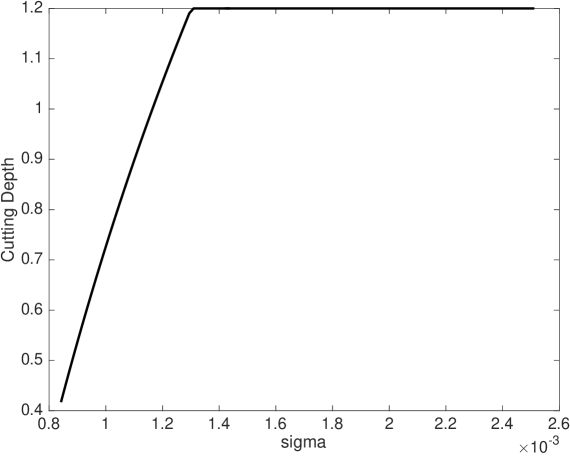
(a) Relationship of optimal cutting depth and $\sigma_{0}$

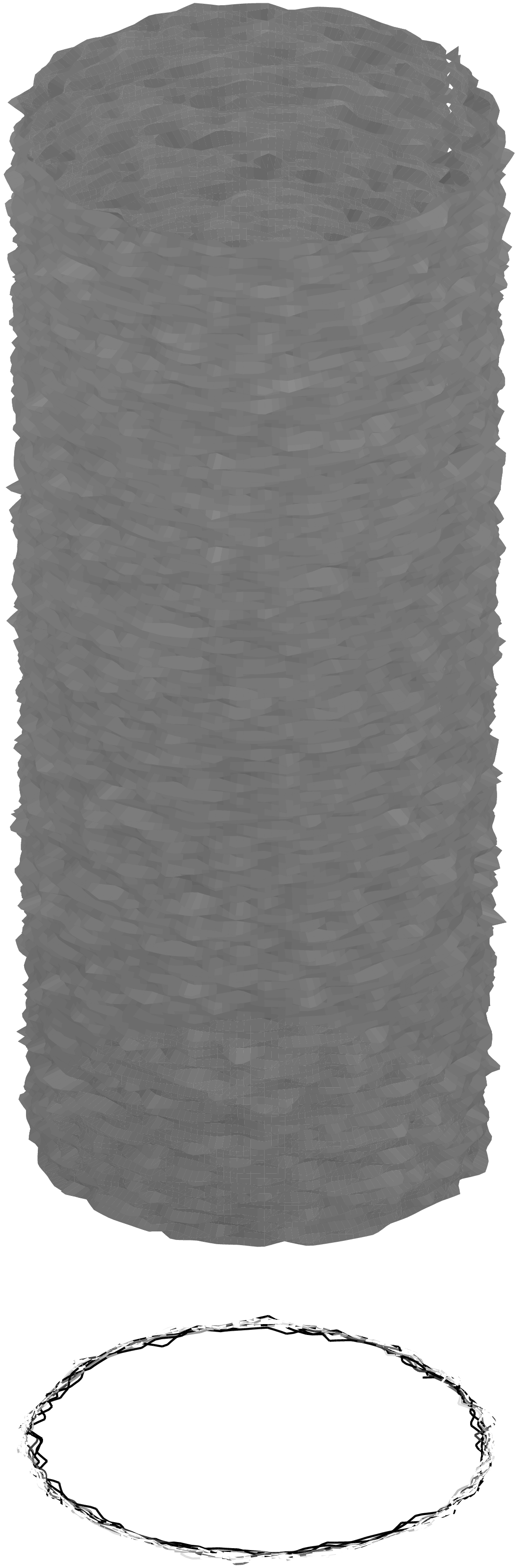
(b) Simulated cylinder under the optimal setting. Scale 250:1

Figure 7: Optimal Settings for different $\sigma$

7 Conclusion

Point cloud modeling is an important research area with various applications especially in modern manufacturing due to the ease of accessibility to 3D scanning tools and the need for accurate shape modeling and control. As most structured point clouds can be represented in a tensor form in a certain coordinate system, in this paper, we proposed to use tensor regression to link the shape of point cloud data with some scalar process variables. However, since the dimensionality of the tensor coefficients in the regression is too high, we suggested to reduce the dimensionality by expanding the tensors on a few sets of basis. To determine the basis, two strategies (i.e. RTR and OTDR) were developed. In the simulation study, we showed both RTR and OTDR outperform the existing vector-based techniques. Finally, the proposed methods were applied to a real case study of the point cloud modeling in a turning process. To model unequal variances due to the roughness, an iterative algorithm for maximum likelihood estimation was proposed which combined the proposed tensor regression model with gamma regression. The results indicated that our methods were capable of identifying the main variational pattern caused by the input variables. We also demonstrated that how this model could be used to find the optimal setting of process variables.

There are several potential research directions to be investigated. One direction is to extend this method to non-smooth point clouds with abrupt changes in surface. Another direction is to develop a modeling approach for unstructured point clouds. Also, the tensor regression problem where both input and response variables are high-order tensors is an interesting, yet challenging problem for future research.

Appendix A Optimizing the Likelihood Function Without Basis

The tensor coefficients can be estimated by minimizing the negative likelihood function $\mathbf{a}$, i.e., $\hat{\mathbf{a}}=\min_{\mathbf{a}}(\mathbf{y}-(\mathbf{X}\otimes I\otimes I)\mathbf{a})^{T}(\Sigma_{3}\otimes\Sigma_{2}\otimes\Sigma_{1})^{-1}(\mathbf{y}-(\mathbf{X}\otimes I\otimes I)\mathbf{a}).$ This can be solved by $\hat{\mathbf{a}}=((\mathbf{X}^{T}\Sigma_{3}^{-1}\mathbf{X})^{-1}\mathbf{X}^{T}\Sigma_{3}^{-1}\otimes I\otimes I)\mathbf{y}$, where $\mathbf{y}=\mathrm{vec}(\mathcal{Y})$ and $\mathbf{a}=\mathrm{vec}(\mathcal{A})$ are the vectorized $\mathcal{Y}$ and $\mathcal{A}$, respectively. This is equivalent to the tensor format equation, which is $\hat{\mathcal{A}}=\mathcal{Y}\times_{3}(\mathbf{X}^{T}\Sigma_{3}^{-1}\mathbf{X})^{-1}\mathbf{X}^{T}\Sigma_{3}^{-1}$.

Appendix B Tucker Decomposition Regression

Principal component analysis (PCA) (Jolliffe,, 2002) has been widely used because of its ability to reduce the dimensionality of high-dimensional data. However, as pointed out by Yan et al., 2015b , applying PCA directly on tensor data requires unfolding the original tensor into a long vector, which may result in the loss of structural information of the original tensor. To address this issue, tensor decomposition techniques such as Tucker decomposition (Tucker,, 1966) have been proposed and widely applied in image denoising, image monitoring, tensor completion, etc. Tucker decomposition aims to find a set of orthogonal transformation matrices $\mathbf{U}=\{\mathbf{U}^{(k)}\in\mathbb{R}^{I_{k}\times P_{k}};\mathbf{U}^{(k)^{T}}\mathbf{U}^{(k)}=\mathbf{I}_{P_{k}},P_{k}<I_{k},k=1,2\}$ such that it can best represents the original data $\mathcal{Y}$, where $\mathbf{I}_{P_{k}}$ represents the identity matrix of size $P_{k}\times P_{k}$. That is,

$$\{\mathcal{\hat{S}},\hat{\mathbf{U}}^{(1)},\hat{\mathbf{U}}^{(2)}\}=\mathop{\mathrm{argmin}}_{\mathcal{S},\mathbf{U}^{(1)},\mathbf{U}^{(2)}}\|\mathcal{Y}-\mathcal{S}\times_{1}\mathbf{U}^{(1)}\times_{2}\mathbf{U}^{(2)}\|_{F}^{2}.$$ (13)

$\mathcal{\hat{S}}$ is the core tensor and can be obtained by

$$\mathcal{\hat{S}}=\mathcal{Y}\times_{1}\hat{\mathbf{U}}^{(1)^{T}}\times_{2}\hat{\mathbf{U}}^{(2)^{T}}.$$ (14)

Yan et al., 2015b showed that (13) is equivalent to maximizing the variation of the projected low-dimensional tensor, known as multi-linear principal component analysis (MPCA) method proposed in (Lu et al.,, 2008). Therefore, for finding the basis matrix, one can solve the following optimization problem:

$$\{\mathbf{\hat{U}}^{(1)},\mathbf{\hat{U}}^{(2)}\}=\mathop{\mathrm{argmax}}_{\mathbf{U}^{(1)},\mathbf{U}^{(2)}}\|\mathcal{Y}\times_{1}\mathbf{U}^{(1)^{T}}\times_{2}\mathbf{U}^{(2)^{T}}\|_{F}^{2}.$$ (15)

$\hat{\mathcal{B}}$ can then be computed by (6) and $\hat{\mathcal{A}}=\hat{\mathcal{B}}\times_{1}\hat{\mathbf{U}}^{(1)}\times_{2}\hat{\mathbf{U}}^{(2)}$.

Appendix C The Proof of Proposition 1

Proof.

The likelihood function can be minimized by:

$$\hat{\boldsymbol{\beta}} =\arg\min_{\boldsymbol{\beta}}(\mathbf{y}-(\mathbf{X}\otimes\mathbf{U}^{(2)}\otimes\mathbf{U}^{(1)})\boldsymbol{\beta})^{T}(\Sigma_{3}\otimes\Sigma_{2}\otimes\Sigma_{1})^{-1}(\mathbf{y}-(\mathbf{X}\otimes\mathbf{U}^{(2)}\otimes\mathbf{U}^{(1)})\boldsymbol{\beta})$$

$$=\arg\min_{\boldsymbol{\beta}}\boldsymbol{\beta}^{T}(\mathbf{X}^{T}\Sigma_{3}^{-1}\mathbf{X}\otimes\mathbf{U}^{(2)T}\Sigma_{2}^{-1}\mathbf{U}^{(2)}\otimes\mathbf{U}^{(1)T}\Sigma_{1}^{-1}\mathbf{U}^{(1)})\boldsymbol{\beta}-2\boldsymbol{\beta}^{T}(\mathbf{X}^{T}\Sigma_{3}^{-1}\otimes\mathbf{U}^{(2)T}\Sigma_{2}^{-1}\otimes\mathbf{U}^{(1)T}\Sigma_{1}^{-1})\mathbf{y}$$

$$=(\mathbf{X}^{T}\Sigma_{3}^{-1}\mathbf{X}\otimes\mathbf{U}^{(2)T}\Sigma_{2}^{-1}\mathbf{U}^{(2)}\otimes\mathbf{U}^{(1)T}\Sigma_{1}^{-1}\mathbf{U}^{(1)})^{-1}(\mathbf{X}^{T}\Sigma_{3}^{-1}\otimes\mathbf{U}^{(2)T}\Sigma_{2}^{-1}\otimes\mathbf{U}^{(1)T}\Sigma_{1}^{-1})\mathbf{y}$$

$$=(\mathbf{X}^{T}\Sigma_{3}^{-1}\mathbf{X})^{-1}\mathbf{X}^{T}\Sigma_{3}^{-1}\otimes(\mathbf{U}^{(2)T}\Sigma_{2}^{-1}\mathbf{U}^{(2)})^{-1}\mathbf{U}^{(2)T}\Sigma_{2}^{-1}\otimes(\mathbf{U}^{(1)T}\Sigma_{1}^{-1}\mathbf{U}^{(1)})^{-1}\mathbf{U}^{(1)T}\Sigma_{1}^{-1}\mathbf{y}$$

Equivalently, this can be written in the tensor format as

$$\hat{\mathcal{B}}=\mathcal{Y}\times_{1}(\mathbf{U}^{(1)T}\Sigma_{1}^{-1}\mathbf{U}^{(1)})^{-1}\mathbf{U}^{(1)T}\Sigma_{1}^{-1}\times_{2}(\mathbf{U}^{(2)T}\Sigma_{2}^{-1}\mathbf{U}^{(2)})^{-1}\mathbf{U}^{(2)T}\Sigma_{2}^{-1}\times_{3}(\mathbf{X}^{T}\Sigma_{3}^{-1}\mathbf{X})^{-1}\mathbf{X}^{T}\Sigma_{3}^{-1}$$

∎

Appendix D The Proof of Proposition 2

Proof.

$\boldsymbol{\beta}$ can be solved by

$$\hat{\boldsymbol{\beta}} =\mathop{argmin}_{\boldsymbol{\beta}}(\mathbf{y}-(\mathbf{X}\otimes\mathbf{U}^{(2)}\otimes\mathbf{U}^{(1)})\boldsymbol{\beta})^{T}(\Sigma_{3}\otimes\Sigma_{2}\otimes\Sigma_{1})^{-1}(\mathbf{y}-(\mathbf{X}\otimes\mathbf{U}^{(2)}\otimes\mathbf{U}^{(1)})\boldsymbol{\beta})+P(\boldsymbol{\beta})$$

$$=\mathop{argmin}_{\boldsymbol{\beta}}\boldsymbol{\beta}^{T}(\mathbf{X}^{T}\Sigma_{3}^{-1}\mathbf{X}\otimes\mathbf{U}^{(2)T}\Sigma_{2}^{-1}\mathbf{U}^{(2)}\otimes\mathbf{U}^{(1)T}\Sigma_{1}^{-1}\mathbf{U}^{(1)})\boldsymbol{\beta}$$

$$+\boldsymbol{\beta}^{T}(\mathbf{X}^{T}\Sigma_{3}^{-1}\mathbf{X})\otimes(\lambda\mathbf{P}_{2}\otimes\mathbf{U}^{(1)^{T}}\mathbf{U}^{(1)}+\lambda\mathbf{U}^{(2)^{T}}\mathbf{U}^{(2)}\otimes\mathbf{P}_{1}+\lambda^{2}\mathbf{P}_{2}\otimes\mathbf{P}_{1})\boldsymbol{\beta}$$

$$-2\boldsymbol{\beta}^{T}(\mathbf{X}^{T}\Sigma_{3}^{-1}\otimes\mathbf{U}^{(2)T}\Sigma_{2}^{-1}\otimes\mathbf{U}^{(1)T}\Sigma_{1}^{-1})\mathbf{y}$$

$$=\mathop{argmin}_{\boldsymbol{\beta}}\boldsymbol{\beta}^{T}(\mathbf{X}^{T}\Sigma_{3}^{-1}\mathbf{X})\otimes(\mathbf{U}^{(2)^{T}}\Sigma_{2}^{-1}\mathbf{U}^{(2)}+\lambda\mathbf{P}_{2})\otimes(\mathbf{U}^{(1)^{T}}\Sigma_{1}^{-1}\mathbf{U}^{(1)}+\lambda\mathbf{P}_{1})$$

$$-2\boldsymbol{\beta}^{T}(\mathbf{X}^{T}\Sigma_{3}^{-1}\otimes\mathbf{U}^{(2)T}\Sigma_{2}^{-1}\otimes\mathbf{U}^{(1)T}\Sigma_{1}^{-1})\mathbf{y}$$

$$=((\mathbf{X}^{T}\Sigma_{3}^{-1}\mathbf{X}\otimes(\mathbf{U}^{(2)^{T}}\Sigma_{2}^{-1}\mathbf{U}^{(2)}+\lambda\mathbf{P}_{2})\otimes(\mathbf{U}^{(1)^{T}}\Sigma_{1}^{-1}\mathbf{U}^{(1)}+\lambda\mathbf{P}_{1}))^{-1}(\mathbf{X}^{T}\Sigma_{3}^{-1}\otimes\mathbf{U}^{(2)T}\Sigma_{2}^{-1}\otimes\mathbf{U}^{(1)T}\Sigma_{1}^{-1})\mathbf{y}$$

$$=(\mathbf{X}^{T}\Sigma_{3}^{-1}\mathbf{X})^{-1}\mathbf{X}^{T}\Sigma_{3}^{-1}\otimes(\mathbf{U}^{(2)^{T}}\Sigma_{2}^{-1}\mathbf{U}^{(2)}+\lambda\mathbf{P}_{2})^{-1}\mathbf{U}^{(2)^{T}}\Sigma_{2}^{-1}\otimes(\mathbf{U}^{(1)^{T}}\Sigma_{1}^{-1}\mathbf{U}^{(1)}+\lambda\mathbf{P}_{1})^{-1}\mathbf{U}^{(1)^{T}}\Sigma_{1}^{-1}\mathbf{y},$$

which is equivalent to solve $\mathcal{B}$ in the tensor format as shown in (9). ∎

Appendix E The Proof of Proposition 3

Proof.

$\beta$ can be solved by

$$\mathop{\mathrm{argmin}}_{\boldsymbol{\beta}}(\mathbf{y}-(\mathbf{X}\otimes\mathbf{U}^{(2)}\otimes\mathbf{U}^{(1)})\boldsymbol{\beta})^{T}(\Sigma_{3}\otimes\Sigma_{2}\otimes\Sigma_{1})^{-1}(\mathbf{y}-(\mathbf{X}\otimes\mathbf{U}^{(2)}\otimes\mathbf{U}^{(1)})\boldsymbol{\beta})$$

$$= \beta^{T}(\mathbf{X}\otimes\mathbf{U}^{(2)}\otimes\mathbf{U}^{(1)})^{T}(\Sigma_{3}\otimes\Sigma_{2}\otimes\Sigma_{1})^{-1}(\mathbf{X}\otimes\mathbf{U}^{(2)}\otimes\mathbf{U}^{(1)})\beta-2\beta^{T}(\mathbf{X}\otimes\mathbf{U}^{(2)}\otimes\mathbf{U}^{(1)})^{T}(\Sigma_{3}\otimes\Sigma_{2}\otimes\Sigma_{1})^{-1}y$$

$\mathbf{y}$ is the vectorized $\mathcal{Y}$ with size $\mathbf{y}\in\mathbb{R^{\mathrm{n_{1}n_{2}N\times 1}}}$, $\boldsymbol{\mathbf{\beta}}$ is the vectorized $\mathcal{B}$ with size $\boldsymbol{\mathbf{\beta}}\in\mathbb{R}^{pI_{1}I_{2}\times 1}$. If we optimize the $\beta$ gives

$$\hat{\beta} =((\mathbf{X}^{T}\Sigma_{3}^{-1}\mathbf{X})^{-1}\mathbf{X}^{T}\Sigma_{3}^{-1}\otimes(\mathbf{U}^{(2)^{T}}\Sigma_{2}^{-1}\mathbf{U}^{(2)})^{-1}\mathbf{U}^{(2)^{T}}\Sigma_{2}^{-1}\otimes(\mathbf{U}^{(1)^{T}}\Sigma_{1}^{-1}\mathbf{U}^{(1)})^{-1}\mathbf{U}^{(1)^{T}}\Sigma_{1}^{-1})\mathbf{y}.$$

$$=((\mathbf{X}^{T}\Sigma_{3}^{-1}\mathbf{X})^{-1}\mathbf{X}^{T}\Sigma_{3}^{-1}\otimes\mathbf{U}^{(2)^{T}}\Sigma_{2}^{-1}\otimes\mathbf{U}^{(1)^{T}}\Sigma_{1}^{-1})\mathbf{y}$$

Or equivalently

$$\hat{\mathcal{B}}=\mathcal{Y}\times_{1}\mathbf{U}^{(1)^{T}}\Sigma_{1}^{-1}\times_{2}\mathbf{U}^{(2)^{T}}\Sigma_{2}^{-1}\times_{3}(\mathbf{X}^{T}\Sigma_{3}^{-1}\mathbf{X})^{-1}\mathbf{X}^{T}\Sigma_{3}^{-1}.$$

Plugging in the estimation of $\hat{\beta}$, we have

$$(\mathbf{y}-(\mathbf{X}\otimes\mathbf{U}^{(2)}\otimes\mathbf{U}^{(1)})\boldsymbol{\hat{\beta}})^{T}(\Sigma_{3}\otimes\Sigma_{2}\otimes\Sigma_{1})^{-1}(\mathbf{y}-(\mathbf{X}\otimes\mathbf{U}^{(2)}\otimes\mathbf{U}^{(1)})\hat{\beta})$$

$$= \hat{\beta}^{T}(\mathbf{X}\otimes\mathbf{U}^{(2)}\otimes\mathbf{U}^{(1)})^{T}(\Sigma_{3}\otimes\Sigma_{2}\otimes\Sigma_{1})^{-1}(\mathbf{X}\otimes\mathbf{U}^{(2)}\otimes\mathbf{U}^{(1)})\hat{\beta}-2\hat{\beta}^{T}(\mathbf{X}\otimes\mathbf{U}^{(2)}\otimes\mathbf{U}^{(1)})^{T}(\Sigma_{3}\otimes\Sigma_{2}\otimes\Sigma_{1})^{-1}y$$

$$= \hat{\beta}^{T}((\mathbf{X}^{T}\Sigma_{3}^{-1}\mathbf{X})\otimes I\otimes I)\hat{\beta}-2\hat{\beta}^{T}(\mathbf{X}^{T}\Sigma_{3}^{-1}\otimes\mathbf{U}^{(2)^{T}}\Sigma_{2}^{-1}\otimes\mathbf{U}^{(1)^{T}}\Sigma_{1}^{-1})y$$

$$= -\mathbf{y}^{T}(\Sigma_{3}^{-1}\mathbf{X}(\mathbf{X}^{T}\Sigma_{3}^{-1}\mathbf{X})^{-1}\mathbf{X}^{T}\Sigma_{3}^{-1})\otimes(\Sigma_{2}^{-1}\mathbf{U}^{(2)}\mathbf{U}^{(2)^{T}}\Sigma_{2}^{-1})\otimes(\Sigma_{1}^{-1}\mathbf{U}^{(1)}\mathbf{U}^{(1)^{T}}\Sigma_{1}^{-1})\mathbf{y}$$

$$= -\|\mathbf{X}_{3}\otimes(\mathbf{U}^{(2)^{T}}\Sigma_{2}^{-1})\otimes(\mathbf{U}^{(1)^{T}}\Sigma_{1}^{-1})\mathbf{y}\|^{2}$$

$$= -\|\mathcal{Y}\times_{1}\mathbf{U}^{(1)^{T}}\Sigma_{1}^{-1}\times_{2}\mathbf{U}^{(2)^{T}}\Sigma_{2}^{-1}\times_{3}\mathbf{X}_{3}\|^{2}$$

∎

This close the first half of the proof. Then we will discuss how to maximize $\|\mathcal{Y}\times_{1}\mathbf{U}^{(1)^{T}}\Sigma_{1}^{-1}\times_{2}\mathbf{U}^{(2)^{T}}\Sigma_{2}^{-1}\times_{3}\mathbf{X}_{3}\|^{2}$ according to the $\mathbf{U}^{(1)}$ and $\mathbf{U}^{(2)}$. We first like to define that $\tilde{\mathbf{U}}^{(k)}=\Sigma_{k}^{-1/2}\mathbf{U}^{(k)}$. The constraint is equivalent to $\tilde{\mathbf{U}}^{(k)T}\tilde{\mathbf{U}}^{(k)}=I$ and the data is$\mathbf{U}^{(k)^{T}}\Sigma_{k}^{-1}=\tilde{\mathbf{U}}^{(k)}\Sigma_{k}^{-1/2}$. The problem becomes

$$\|\mathcal{Y}\times_{1}\mathbf{U}^{(1)^{T}}\Sigma_{1}^{-1}\times_{2}\mathbf{U}^{(2)^{T}}\Sigma_{2}^{-1}\times_{3}\mathbf{X}_{3}\|^{2}$$

$$= \|\mathcal{W}_{k}\times_{k}\tilde{\mathbf{U}}^{(k)}\Sigma_{k}^{-1/2}\|^{2}$$

$$= \|\tilde{\mathbf{U}}^{(k)}\Sigma_{k}^{-1/2}\mathbf{W}_{k}\|^{2}$$

Here $W_{k}$ is the $k^{th}$ mode unfolding of $\mathcal{W}_{k}=\mathcal{Y}\times_{i}\mathbf{U}^{(i)}\Sigma_{i}^{-1}\times_{3}X_{3}$. It is not hard to prove that $\max_{\tilde{\mathbf{U}}^{(k)}}\|\tilde{\mathbf{U}}^{(k)}\Sigma_{k}^{-1/2}\mathbf{W}_{k}\|^{2}$ s.t. $\tilde{\mathbf{U}}^{(k)T}\tilde{\mathbf{U}}^{(k)}=I$ can be solved by the first $P_{k}$ eigenvectors of $\Sigma_{k}^{-1/2}\mathbf{W}_{k}$.

References

- Anandkumar et al., (2013) Anandkumar, A., Hsu, D. J., Janzamin, M., and Kakade, S. M. (2013). When are overcomplete topic models identifiable? uniqueness of tensor tucker decompositions with structured sparsity. In Advances in neural information processing systems, pages 1986–1994.
- Baumgart, (1975) Baumgart, B. (1975). Winged-edge polyhedron representation for computer vision. national computer conference, may 1975.
- Bernardini et al., (1999) Bernardini, F., Mittleman, J., Rushmeier, H., Silva, C., and Taubin, G. (1999). The ball-pivoting algorithm for surface reconstruction. IEEE transactions on visualization and computer graphics, 5(4):349–359.
- Chauhan and Dass, (2012) Chauhan, S. R. and Dass, K. (2012). Optimization of machining parameters in turning of titanium (grade-5) alloy using response surface methodology. Materials and Manufacturing Processes, 27(5):531–537.
- Colosimo et al., (2014) Colosimo, B. M., Cicorella, P., Pacella, M., and Blaco, M. (2014). From profile to surface monitoring: Spc for cylindrical surfaces via gaussian processes. Journal of Quality Technology, 46(2):95–113.
- Colosimo et al., (2010) Colosimo, B. M., Mammarella, F., and Petro, S. (2010). Quality control of manufactured surfaces. In Frontiers in Statistical Quality Control 9, pages 55–70. Springer.
- Colosimo and Pacella, (2011) Colosimo, B. M. and Pacella, M. (2011). Analyzing the effect of process parameters on the shape of 3d profiles. Journal of Quality Technology, 43(3).
- Edelsbrunner and Mücke, (1994) Edelsbrunner, H. and Mücke, E. P. (1994). Three-dimensional alpha shapes. ACM Transactions on Graphics (TOG), 13(1):43–72.
- Gibson et al., (2010) Gibson, I., Rosen, D. W., Stucker, B., et al. (2010). Additive manufacturing technologies, volume 238. Springer.
- Helland, (1990) Helland, I. S. (1990). Partial least squares regression and statistical models. Scandinavian Journal of Statistics, pages 97–114.
- Henke et al., (1999) Henke, R., Summerhays, K., Baldwin, J., Cassou, R., and Brown, C. (1999). Methods for evaluation of systematic geometric deviations in machined parts and their relationships to process variables. Precision Engineering, 23(4):273 – 292.
- Jolliffe, (2002) Jolliffe, I. (2002). Principal component analysis. Wiley Online Library.
- Khanna and Davim, (2015) Khanna, N. and Davim, J. (2015). Design-of-experiments application in machining titanium alloys for aerospace structural components. Measurement, 61:280 – 290.
- Kolda and Bader, (2009) Kolda, T. G. and Bader, B. W. (2009). Tensor decompositions and applications. SIAM review, 51(3):455–500.
- Li and Zhang, (2016) Li, L. and Zhang, X. (2016). Parsimonious tensor response regression. Journal of the American Statistical Association, (just-accepted).
- Li et al., (2011) Li, Y., Zhu, H., Shen, D., Lin, W., Gilmore, J. H., and Ibrahim, J. G. (2011). Multiscale adaptive regression models for neuroimaging data. Journal of the Royal Statistical Society: Series B (Statistical Methodology), 73(4):559–578.
- Lu et al., (2008) Lu, H., Plataniotis, K. N., and Venetsanopoulos, A. N. (2008). Mpca: Multilinear principal component analysis of tensor objects. Neural Networks, IEEE Transactions on, 19(1):18–39.
- Manceur and Dutilleul, (2013) Manceur, A. M. and Dutilleul, P. (2013). Maximum likelihood estimation for the tensor normal distribution: Algorithm, minimum sample size, and empirical bias and dispersion. Journal of Computational and Applied Mathematics, 239:37–49.
- Pacella and Colosimo, (2016) Pacella, M. and Colosimo, B. M. (2016). Multilinear principal component analysis for statistical modeling of cylindrical surfaces: a case study. Quality Technology and Quantitative Management, In press.
- Peng et al., (2010) Peng, J., Zhu, J., Bergamaschi, A., Han, W., Noh, D.-Y., Pollack, J. R., and Wang, P. (2010). Regularized multivariate regression for identifying master predictors with application to integrative genomics study of breast cancer. The annals of applied statistics, 4(1):53.
- Penny et al., (2011) Penny, W. D., Friston, K. J., Ashburner, J. T., Kiebel, S. J., and Nichols, T. E. (2011). Statistical parametric mapping: the analysis of functional brain images. Academic press.
- Pervaiz et al., (2014) Pervaiz, S., Rashid, A., Deiab, I., and Nicolescu, M. (2014). Influence of tool materials on machinability of titanium- and nickel-based alloys: A review. Materials and Manufacturing Processes, 29(3):219–252.
- Peters et al., (2003) Peters, M., Kumpfert, J., Ward, C., and Leyens, C. (2003). Titanium alloys for aerospace applications. Advanced Engineering Materials, 5(6):419–427.
- Pieraccini et al., (2001) Pieraccini, M., Guidi, G., and Atzeni, C. (2001). 3d digitizing of cultural heritage. Journal of Cultural Heritage, 2(1):63–70.
- Pramanik, (2014) Pramanik, A. (2014). Problems and solutions in machining of titanium alloys. The International Journal of Advanced Manufacturing Technology, 70(5):919–928.
- Ramesh et al., (2012) Ramesh, S., Karunamoorthy, L., and Palanikumar, K. (2012). Measurement and analysis of surface roughness in turning of aerospace titanium alloy (gr5). Measurement, 45(5):1266 – 1276.
- Reiss et al., (2010) Reiss, P. T., Huang, L., and Mennes, M. (2010). Fast function-on-scalar regression with penalized basis expansions. The international journal of biostatistics, 6(1).
- Rogers, (2000) Rogers, D. F. (2000). An introduction to NURBS: with historical perspective. Elsevier.
- Shewchuk, (1996) Shewchuk, J. R. (1996). Triangle: Engineering a 2d quality mesh generator and delaunay triangulator. In Applied computational geometry towards geometric engineering, pages 203–222. Springer.
- Silverman, (1995) Silverman, B. W. (1995). Incorporating parametric effects into functional principal components analysis. Journal of the Royal Statistical Society. Series B (Methodological), pages 673–689.
- Tucker, (1966) Tucker, L. R. (1966). Some mathematical notes on three-mode factor analysis. Psychometrika, 31(3):279–311.
- Wells et al., (2013) Wells, L. J., Megahed, F. M., Niziolek, C. B., Camelio, J. A., and Woodall, W. H. (2013). Statistical process monitoring approach for high-density point clouds. Journal of Intelligent Manufacturing, 24(6):1267–1279.
- Western and Bloome, (2009) Western, B. and Bloome, D. (2009). Variance function regressions for studying inequality. Sociological Methodology, 39(1):293–326.
- Xiao et al., (2013) Xiao, L., Li, Y., and Ruppert, D. (2013). Fast bivariate p-splines: the sandwich smoother. Journal of the Royal Statistical Society: Series B (Statistical Methodology), 75(3):577–599.
- (35) Yan, H., Paynabar, K., and Shi, J. (2015a). Anomaly detection in images with smooth background via smooth-sparse decomposition. Technometrics, (just-accepted):00–00.
- (36) Yan, H., Paynabar, K., and Shi, J. (2015b). Image-based process monitoring using low-rank tensor decomposition. Automation Science and Engineering, IEEE Transactions on, 12(1):216–227.
- Zhang et al., (2005) Zhang, X. D., Zhang, C., Wang, B., and Feng, S. C. (2005). Unified functional approach for precision cylindrical components. International Journal of Production Research, 43(1):25–47.
- Zhou et al., (2013) Zhou, H., Li, L., and Zhu, H. (2013). Tensor regression with applications in neuroimaging data analysis. Journal of the American Statistical Association, 108(502):540–552.