Traces of exomoons in
computed flux and polarization phase curves
of starlight reflected by exoplanets

Abstract

Context. Detecting moons around exoplanets is a major goal of current and future observatories. Moons are suspected to influence rocky exoplanet habitability, and gaseous exoplanets in stellar habitable zones could harbor abundant and diverse moons to target in the search for extraterrestrial habitats. Exomoons will contribute to exoplanetary signals but are virtually undetectable with current methods.

Aims. We identify and analyze traces of exomoons in the temporal variation of total and polarized fluxes of starlight reflected by an Earth–like exoplanet and its spatially unresolved moon across all phase angles, with both orbits viewed in an edge–on geometry.

Methods. We compute the total and linearly polarized fluxes, and the degree of linear polarization $P$ of starlight that is reflected by the exoplanet with its moon along their orbits, accounting for the temporal variation of the visibility of the planetary and lunar disks, and including effects of mutual transits and mutual eclipses. Our computations pertain to a wavelength of 450 nm.

Results. Total flux $F$ shows regular dips due to planetary and lunar transits and eclipses. Polarization $P$ shows regular peaks due to planetary transits and lunar eclipses, and $P$ can increase and/or slightly decrease during lunar transits and planetary eclipses. Changes in $F$ and $P$ will depend on the radii of the planet and moon, on their reflective properties, and their orbits, and are about one magnitude smaller than the smooth background signals. The typical duration of a transit or an eclipse is a few hours.

Conclusions. Traces of an exomoon due to planetary and lunar transits and eclipses show up in $F$ and $P$ of sunlight reflected by planet–moon systems and could be searched for in exoplanet flux and/or polarization phase functions.

1 Introduction

Since the detection of the first planets beyond our Solar System (Wolszczan & Frail, 1992; Campbell et al., 1988), the number of discoveries has steadily increased, yielding almost 4000 confirmed exoplanets and 2500 unconfirmed, candidate exoplanets to this day (Han et al., 2014). Exoplanet space telescopes, such as ESA’s CHEOPS (CHaracterising ExOPlanet Satellite) and Plato (PLAnetary Transits and Oscillations of stars), and NASA’s Transiting Exoplanet Survey Satellite (TESS), are dedicated to find exoplanets around bright, nearby stars. The relative small distances to these stars and their planets combined with the high sensitivity of these missions and the upcoming JWST/NASA (James Webb Space Telescope) and ARIEL/ESA (Tinetti et al., 2016) missions will allow the search for lunar companions and planetary rings.

The continuous increase in instrument precision, stability and spatial resolution has enabled a new generation of ground–based instruments, such as the Gemini Planet Imager (GPI) instrument (see Macintosh et al., 2014) on the Gemini North telescope, the Spectro–Polarimetric High–contrast Exoplanet Research (SPHERE) instrument (see Beuzit et al., 2006) on ESO’s Very Large Telescope (VLT) and the proposed Exoplanet Imaging Camera and Spectrograph (EPICS) (see Keller et al., 2010; Gratton et al., 2010) on the European Extremely Large Telescope (E-ELT), which is under construction by ESO. These high–contrast instruments use direct imaging of planetary radiation to not only detect but also characterize exoplanetary systems through a combination of spectroscopy and polarimetry techniques. Using GPI and SPHERE, respectively, Macintosh et al. (2015) and Wagner et al. (2016) announced the discoveries of young, and thus hot Jovian planets, whose atmospheric properties and orbits were characterized using near–infrared spectroscopy.

Direct detection of extrasolar bodies presents a major challenge as their observed radiation, both emitted and reflected, is very weak compared to that of the host star. In addition, the angular distance from the planet to the star is extremely small. Consequently, the vast majority of exoplanets have only been detected indirectly. In contrast, direct imaging of the planet can reveal a wealth of information of the planet properties that cannot be obtained through other methods, such as lower atmospheric composition and, for rocky planets, their surface coverage.

Despite not having been exploited yet, great hope is placed in the polarimetry capabilities of current and future telescopes as powerful tools for detecting and characterizing exoplanets (see Snik & Keller, 2013; Stam et al., 2004; Seager et al., 2000; Hough et al., 2003; Hough & Lucas, 2003; Saar & Seager, 2003; Stam, 2003, 2008). Previous works in this field involve the modeling of stellar polarization during planetary transits (Wiktorowicz & Laughlin, 2014; Kostogryz et al., 2011, 2015; Sengupta, 2016; Carciofi & Magalhães, 2005), the modeling of light curves and polarization of starlight reflected signals in the visible range of Earth-like planets (Rossi & Stam, 2017; Karalidi et al., 2012; Stam, 2008), and giant Jupiter-like planets (Stam et al., 2004; Seager et al., 2000), as well as the modeling of exoplanetary atmospheres in the infrared (De Kok et al., 2011; Marley & Sengupta, 2011), which demonstrated the usefulness of direct observations on exoplanet characterization. More recently, Bott et al. (2016) reported linear polarization observations of the hot Jupiter system HD 189733, and Ginski et al. (2018) announced the detection of planetary thermal radiation that is polarized upon reflection by circumstellar dust. Indeed, polarization has also been proposed as a means for exomoon detection: Sengupta & Marley (2016) studied the effects of a satellite transiting its hot host planet in the polarization signal of (infrared) thermally emitted radiation for the case of homogeneous, spherically symmetric cloudy planets. Studying exomoons can improve our understanding of in particular:

1. Planet formation: Solar System moons appear to support diverse formation histories. For instance, Titan might have formed from circumplanetary debris, while the Moon, Phobos and Deimos suggest a cumulative bombardment (Rufu et al., 2017; Rosenblatt et al., 2016). Triton might have been captured by Neptune (Agnor & Hamilton, 2006), while collisions are thought to have altered the relative alignment between Uranus and its moons (Morbidelli et al., 2012). Indeed, studying Solar System moons gives essential insights on formation mechanisms and evolution (see Heller, 2017, and references therein). Exomoon research would allow refining planet formation theories in a way not achievable by studying exoplanets alone.

2. Extra-solar system characterization: studying exomoons will not only provide information on lunar orbits and physical properties, but will also allow constraining planet characteristics such as i.e. mass, oblateness, and rotation axis (Barnes & Fortney, 2003; Kipping et al., 2009; Schneider et al., 2015). A signal of a planet-moon system could be interpreted as that of a planet alone, resulting in e.g. an overestimation of the planet mass and effective temperature (Williams & Knacke, 2004), and/or an anomalous composition from spectroscopy (Schneider et al., 2015). Extrasolar system characterization would indeed require analysis of all of its elements, i.e. planets, moons, rings, and exozodiacal dust.

3. Exoplanet and exomoon habitability: a moon may influence its planet’s habitability (Benn, 2001), and moons of giant exoplanets within the stellar habitable zone (HZ) might host habitable environments (Canup & Ward, 2006). Reynolds et al. (1987) and Heller & Barnes (2015) mention the role of a moon’s orbit on the presence of liquid, life–supporting water. Indeed, tidal heating could maintain surface temperatures compatible with life on large moons around cold giant planets (Scharf, 2006). Lehmer et al. (2017) show that small moons could retain atmospheres over limited time periods, while Ganymede–sized moons in a stellar HZ could hold atmospheres and surface water indefinitely. Although radiation in a giant planet’s magnetic field and eclipses could threaten local conditions for life (Heller & Barnes, 2013; Heller, 2012; Forgan & Yotov, 2014), exomoons are interesting targets in the search for extraterrestrial life.

Led by Kipping’s Hunt for Exomoons with Kepler, which uses a combination of photometric transits, Transit Timing Variations (TTV) and Transit Duration Variations (TDV) data (Kipping et al., 2015; Kipping, 2009; Sartoretti & Schneider, 1999; Szabó et al., 2006; Simon et al., 2007, 2015), and Hippke’s search using the Orbital Sampling Effect (OSE) (Hippke, 2015; Heller, 2014; Heller et al., 2016), the search for exomoons is in its starting phase. Mars–sized and possibly even Ganymede-sized satellites could be traceable in archived Kepler data (Heller et al., 2014). Unfortunately, as of yet no exomoons have been confirmed.

In this paper, we use numerical simulations to show how an exomoon could influence the flux and degree of polarization of the starlight that is reflected by an Earth-like exoplanet, using the following outline. In Sect. 2, we describe the numerical code to compute the various geometries of the exoplanet–exomoon system that are required for our radiative transfer computations and the radiative transfer code to compute the reflected fluxes and polarization for a given exoplanet–exomoon system. In Sect. 3, we present computed flux and polarization phase functions at 450 nm, for an Earth-like planet (with a Lambertian reflecting surface and a gaseous atmosphere) with a Moon–like satellite (with a Lambertian reflecting surface) in an edge–on geometry. Finally, in Sect. 4, we summarize and discuss our findings and their implications.

2 Computing the reflected starlight

2.1 Stokes vectors and polarization

We describe the flux and polarization of starlight that is reflected by a body, with a Stokes vector (see e.g. Hansen & Travis, 1974):

$$\mathbf{F}=\left[{\begin{array}[]{*{20}{c}}F\\ Q\\ U\\ V\end{array}}\right],$$ (1)

with $F$ the total flux, $Q$ and $U$ the linearly polarized fluxes, and $V$ the circularly polarized flux, all with dimensions W m^-2. In principle, these fluxes are wavelength dependent. However, we will not explicitly include the wavelength in the dimensions, because we focus on a single wavelength region. Fluxes $Q$ and $U$ are defined with respect to a reference plane, for which we use the planetary (or lunar) scattering plane, which contains the observer, and the centers of the planet (or moon) and the star. We do not compute the circularly polarized flux $V$, because it is usually much smaller than the linearly polarized fluxes (see Rossi & Stam, 2018; Kawata, 1978; Hansen & Travis, 1974), and because ignoring $V$ does not lead to significant errors in the computation of $F$, $Q$, and $U$ (see Stam & Hovenier, 2005). The light of the star is assumed to be unpolarized (see Kemp et al., 1987), and is given by $\mathbf{F}_{\rm 0}=F_{0}\mathbf{1}$, with $\mathbf{1}$ the unit column vector and $\pi F_{0}$ the flux measured perpendicular to the light’s propagation direction. If the orbit of the barycenter of the planet–moon system around the star is eccentric, the incident flux varies along the orbit. Our standard stellar flux, $\pi F_{0}$, is defined with respect to the periapsis of the orbit of the system’s barycenter.

The degree of linear polarization, $P$, of vector $\mathbf{F}$ is defined as

$$P=\sqrt{Q^{2}+U^{2}}/F,$$ (2)

and the direction of polarization, $\chi$, with respect to the reference plane can be computed from

$$\tan{2\chi}=U/Q,$$ (3)

where $\chi$ is chosen such that $0\leq\chi<\pi$, while $\cos{2\chi}$ and $Q$ have the same sign (Hansen & Travis, 1974; Hovenier et al., 2004).

2.2 Disk–integrated reflected Stokes vectors

We compute the reflected Stokes vector $\mathbf{F}$ of the spatially unresolved planet–moon system as a summation of the reflected Stokes vectors $\mathbf{F}^{\rm p}$ and $\mathbf{F}^{\rm m}$ of, respectively, the planet and the moon (the pair is spatially resolved from the star):

$$\mathbf{F}=\hskip 1.42271pt\mathbf{F}^{\rm p}+\frac{R^{2}_{\rm m}}{R^{2}_{\rm p}}\hskip 1.42271pt\mathbf{L}(\psi)\hskip 1.42271pt\mathbf{F}^{\rm m}.$$ (4)

Vectors $\mathbf{F}^{\rm p}$ and $\mathbf{F}^{\rm m}$ are disk–integrated vectors that include the effects of eclipses and transits. They are normalized such that the total fluxes reflected by the planet and moon at a phase angle $\alpha=0^{\circ}$ and without shadows and/or eclipses on their disks, equal the planet’s and moon’s geometric albedo’s, respectively (see Stam et al., 2006). Furthermore, $R_{\rm p}$ and $R_{\rm m}$ are the radii of the (spherical) planet and moon, respectively.

Vectors $\mathbf{F}$ and $\mathbf{F}^{\rm p}$ in Eq. 4 are defined with respect to the planetary scattering plane, while $\mathbf{F}^{\rm m}$ is defined with respect to the lunar scattering plane. Depending on the orientation of the lunar orbit, the lunar scattering plane can have a different orientation than the planetary scattering plane. Matrix ${\bf L}$ in Eq. 4 rotates $\mathbf{F}^{\rm m}$ from the lunar to the planetary scattering plane. It is given by (see Hovenier & van der Mee, 1983)

$$\mathbf{L}(\psi)=\left[{\begin{array}[]{*{20}{c}}1&0&0&0\\ 0&{\cos{2\psi}}&{\sin{2\psi}}&0\\ 0&{\sin{2\psi}}&{\cos{2\psi}}&0\\ 0&0&0&1\end{array}}\right]\,,$$ (5)

with $\psi$ the rotation angle measured in the clockwise direction from the lunar to the planetary scattering plane when looking towards the moon ($0\leq\psi<\pi$).

Figure 1: 3D–view (left) and projection onto the $x_{0}-y_{0}$ plane (right) of the discretized planet or moon. The $z_{0}$–axis points towards the observer. The orientation of the $x_{0}$ and $y_{0}$ axes with respect to the disk of the planet or moon can be chosen arbitrarily.

To compute the disk–integrated vectors $\mathbf{F}^{\rm p}$ and $\mathbf{F}^{\rm m}$, we divide the disks of the planet and the moon as seen by the observer, into a grid of equally sized, square pixels (see Fig. 1). The number of pixels on the planetary disk is $N_{\rm p}$ and that on the lunar disk $N_{\rm m}$. A given pixel will contribute to a disk–signal when its center is within the disk–radius. Obviously, the larger the number of pixels (and the smaller each pixel), the better the approximation of the curved limb of the disk, the terminator, and the shadows, such as those due to eclipses (see App. C for insight into the effect of the number of pixels on the computed signals). The disk–integrated vectors are obtained by summing up the contributions of the individual pixels across the disk, fully taking into account shadows and eclipses, i.e.

$${\mathbf{F}}^{\rm x}=\frac{\pi}{N_{\rm x}}\hskip 1.42271pt\displaystyle\sum_{i=1}^{N_{\rm x}}b_{i}\hskip 1.42271ptc_{i}\hskip 1.42271ptd_{i}\hskip 1.42271pt\mathbf{L}(\beta_{i})\hskip 1.42271pt\mathbf{F}^{\rm x}_{i},$$ (6)

where ’x’ is either ’p’ or ’m’. Factor $\pi/N_{\rm x}$ is the surface area per pixel. Furthermore, ${\mathbf{F}}^{\rm x}_{i}$ is the reflected Stokes vector for the $i$-th pixel on the planet (x=p) or moon (x=m), the computation of which is described in Sect. 2.3. Matrix $\mathbf{L}$ is a rotation matrix (see Eq. 5) that is used for rotating the local Stokes vector ${\mathbf{F}}^{\rm x}_{i}$ that is defined with respect to the local reference plane, to the planetary or lunar scattering plane. Factor $b_{i}$ accounts for the visibility of pixel $i$: if $b_{i}=1$, the pixel is visible to the observer, and if $b_{i}=0$ it is invisible due to a transiting body. Factor $c_{i}$ accounts for the dimming of the local incident stellar flux due to a (partial) eclipse: $c_{i}=0.0$ indicates that pixel $i$ is eclipsed and receives no flux, and $c_{i}=1.0$ indicates that the pixel is not eclipsed. For partial (penumbral) eclipses, $0.0<c_{i}<1.0$. The computation of factors $b_{i}$ and $c_{i}$ is described in Sect. 2.4. Factor $d_{i}$, finally, indicates the decrease of the standard incident stellar flux $\pi F_{0}$ due to an increase of the distance to the star, according to

$$d_{i}=\left(r_{\rm ref}/r_{i{\rm s}}\right)^{2},$$ (7)

where $r_{\rm ref}$ is the reference distance at which the standard stellar flux is defined and $r_{i{\rm s}}$ is the actual distance between pixel $i$ and the star.

2.3 The locally reflected starlight

The Stokes vector of the starlight that is reflected by pixel $i$ on the planet or moon is computed using (see Hansen & Travis, 1974):

$${\mathbf{F}_{i}^{\rm x}}(\theta_{i},\theta_{0i},\phi_{i}-\phi_{0i})=\cos{\theta_{0i}}\leavevmode\nobreak\ {\bf\mathbf{R}}_{1i}^{\rm x}(\theta_{i},\theta_{0i},\phi_{i}-\phi_{0i})\leavevmode\nobreak\ F_{0},$$ (8)

with $\theta_{i}$ the angle between the local zenith direction and the local direction to the observer, $\theta_{0i}$ the angle between the local zenith direction and the local direction to the star, and $\phi_{i}-\phi_{0i}$ the local azimuthal difference angle, i.e. the angle between the plane containing the local zenith direction and the local direction to the observer and the plane containing the local zenith direction and the local direction to the star (see Rossi et al., 2018; de Haan et al., 1987). Furthermore, ${\mathbf{R}}^{\rm x}_{1i}$ is the first column of the local reflection matrix of the planet or moon. Only the first column is needed because the incident starlight is assumed to be unpolarized (cf. Sect. 2.1). For a given pixel, the illumination and viewing angles, and thus $\mathbf{R}^{\rm x}_{1i}$, depend on the position of the planet or moon with respect to the star and to each other. Local reflection matrix $\mathbf{R}^{\rm x}_{i}$ also depends on the local composition and structure of the atmosphere and/or surface of the reflecting body. We compute reflected starlight for an Earth–Moon–like planetary system, keeping the reflection models for the Earth and the moon simple to avoid introducing too many details that increase computational times while not adding insight into the observable signals.

Our model planet has a flat, Lambertian (i.e. isotropically and depolarizing) reflecting surface with an albedo, $a_{\rm surf}$, of 0.3. The surface is overlaid by an atmosphere that is assumed to consist of only gas. We compute the atmospheric optical thickness at a given wavelength $\lambda$, using a model atmosphere consisting of 32 layers, with the ambient pressure and temperature according to a mid-latitude summer profile McClatchey et al. (1972). The surface pressure is 1.0 bars. The molecular scattering optical thickness $b^{\rm m}_{\rm sca}$ of an atmospheric layer at wavelength $\lambda$ is calculated according to

$$b^{\rm m}_{\rm sca}(\lambda)=\sigma^{\rm m}_{\rm sca}(\lambda)\hskip 5.69046ptN,$$ (9)

with $\sigma^{\rm m}_{\rm sca}$ the molecular scattering cross–section (in m²) and $N$ the molecular column number density (in m^-2) of the atmospheric layer. The molecular scattering cross–section is calculated according to

$$\sigma^{\rm m}_{\rm sca}(\lambda)=\frac{24\pi^{3}}{N_{\rm L}^{2}}\frac{(n(\lambda)^{2}-1)^{2}}{(n(\lambda)^{2}+2)^{2}}\frac{6+3\delta(\lambda)}{6-7\delta(\lambda)}\frac{1}{\lambda^{4}},$$ (10)

with $N_{\rm L}$, Loschmidt’s number at standard pressure and temperature, $n$, the wavelength dependent refractive index of dry air under standard pressure and temperature, and $\delta$, the depolarization factor of the atmospheric gas (see Stam, 2008, and references therein for the values that have been chosen for the various parameters). To calculate the molecular column number density $N$, we assume hydrostatic equilibrium in each atmospheric layer, thus

$$N=\frac{\delta p}{mg},$$ (11)

with $\Delta p$ the difference between the pressure at the bottom and at the top of the atmospheric layer (in Pa), $m$ the average molecular mass in the layer (in kg), and $g$ the acceleration of gravity (in m s^-2). The atmospheric optical thickness at a given wavelength $\lambda$ is calculated by adding the values of $b^{\rm m}_{\rm sca}$ for all atmospheric layers at that wavelength (note that for a model atmosphere containing only gas, the radiative transfer of incident sunlight only depends on the total optical thickness, not on the vertical distribution of the optical thickness). The total atmospheric optical thickness at 450 nm, the wavelength of our interest, is 0.14. At this wavelength, there is no significant absorption by atmospheric gases in the Earth’s atmosphere (see Stam, 2008, for sample spectra). The single scattering albedo of the gaseous molecules can thus be assumed to equal 1.0. And, at this short wavelength, the horizontal inhomogeneities of the Earth’s surface and the contributions of clouds and aerosol to the reflected signal are relatively small (see Stam, 2008, for simulations of the Earth’s signal at 440 nm). Our model moon has no atmosphere above its flat, Lambertian (i.e. isotropic and depolarizing) reflecting surface with $a_{\rm surf}=0.1$ (Williams, 2017).

The computation of the local illumination and viewing geometries $\theta_{i}$, $\theta_{0i}$, and $\phi_{i}-\phi_{0i}$ is described in Appendix A. Given these angles and the planet’s atmosphere–surface model, we use PyMieDAP (Rossi et al., 2018), an efficient radiative transfer code based on the adding–doubling algorithm described by de Haan et al. (1987). PyMieDAP fully includes polarization for all orders of scattering, and assumes a locally plane–parallel atmosphere–surface model to compute ${\mathbf{R}}_{1i}^{\rm p}$ for every pixel on the planet. The computed locally reflected Stokes vector, ${\mathbf{F}_{i}}^{\rm p}$, is defined with respect to the local meridian plane, i.e. the plane through the local zenith and the local direction towards the observer. For each illuminated pixel on the moon, ${\mathbf{R}}_{1i}^{\rm m}=a_{\rm surf}\mathbf{1}$. A detailed description of PyMieDAP including benchmark results can be found in Rossi et al. (2018).

Results of our radiative transfer code have been compared against results presented in e.g. Stam (2008); Stam et al. (2006, 2004) (who all used the same adding–doubling code, but an entirely different disk–integration algorithm), and Karalidi et al. (2012) (who used their own version of an adding–doubling code and an independent disk–integration method). Buenzli & Schmid (2009) and Stolker et al. (2017), each compared their own, independently implemented Monte Carlo radiative transfer codes successfully against results from the code used by Stam et al. (2004) and Stam et al. (2006).

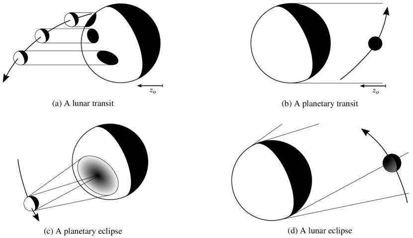
Figure 2: Sketch illustrating the mutual events between a planet and its moon: (a) a lunar transit, (b) a planetary transit, (c) a planetary eclipse, and (d) a lunar eclipse. The positive $z_{0}$–axis (in sub-figures a and b) points to the observer. The white–black scale indicates full–null illumination of a body. An arrow indicates the lunar motion around the planet. The distances and radii are not to scale.

2.4 Computing transits and eclipses

As described in Eq. 6, the contribution of the light reflected by a pixel $i$ on the planet or the moon to the disk–integrated Stokes vector $\mathbf{F}$, depends on the factors $b_{i}$ and $c_{i}$, that account for the pixel’s visibility and dimming, respectively. The values of these factors depend on so–called mutual events, specifically, transits, in which one body is (partially) blocking the light that is reflected towards the observer by another body, and eclipses, in which one body is casting a (partial) shadow on the illuminated and visible disk of another body. Limiting ourselves to systems in which a single star is orbited by a planet with a single moon, we distinguish the following four mutual events (cf. Fig. 2):

1. A planetary eclipse: the moon is between the star and the planet, casting its shadow on the planet, the extent of which depends on the planet–star and moon–star distances, on the stellar, planetary and lunar radii, and on their orbital positions.

2. A lunar eclipse: the planet is between the star and the moon, casting its shadow on the moon, the extent of which depends on the planet–star and moon–star distances, on the stellar, planetary and lunar radii, and on their orbital positions.

3. A planetary transit: the planet is between the moon and the observer, blocking the view of the moon, the extent of which depends on the planetary and lunar radii, and their orbital positions.

4. A lunar transit: the moon is between the planet and the observer, occulting a region of the planetary disk, the extent of which depends on the planetary and lunar radii, and their orbital positions.

We exclude planetary and lunar transits of the star, i.e. the epochs in which these bodies move in front or behind the star. Numerical simulations of transiting planets with moons have been published by Kipping (2011). Modeling the transmission and scattering of starlight in the planetary atmosphere during those epochs (which is not included in the work by Kipping (2011)), requires a fully spherical atmosphere model instead of a locally plane-parallel one (de Kok & Stam, 2012) and falls outside the scope of this paper.

For our computation of the effects of transits of the planet in front of the moon and vice versa on the flux and polarization of the reflected starlight, we assume that the bodies are at ’infinite’ distance of the observer. For our computation of the effects of the eclipses, i.e. the shadow of one body darkening regions on the other body, on the reflected flux and polarization, we follow the mathematical description of eclipses in the Moon–Earth system as developed by Link (1969), taking into account the sizes of the planet and the moon, their distances and positions with respect to the star, and the size of the stellar disk. The latter is crucial for the modeling of the umbra, antumbra en penumbra shadow regions (for an example of the umbra and penumbra, see Fig. 2). The contribution of the starlight reflected by pixels in the antumbral or penumbral region of the planet or moon to the total signal is weighted by the depth of the shadow (i.e. factor $c_{i}$ in Eq. 6). We ignore stellar limb darkening and the transmission of starlight through the planetary atmosphere during a lunar eclipse.

A detailed description of our numerical computation of eclipses and the factor $c_{i}$ in Eq. 6 is provided in Appendix B. This computation requires the positions of the planet and the moon with respect to the star across time, and thus the dynamics of the three–body system. The basics of this dynamics is outlined in the next section.

2.5 Computing the orbits of the planet & moon

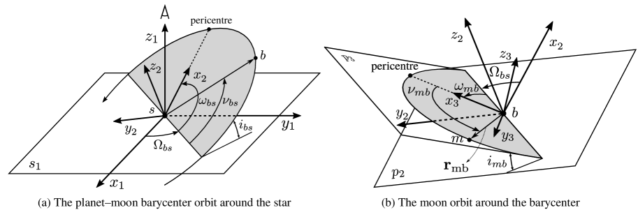
Figure 3: Sketch of the reference frames and angles used to describe the Keplerian orbits of the planet–moon system barycenter around the parent star (Fig. a) and the Keplerian orbit of the moon around the planet–moon system barycenter (Fig. b). Plane $p_{1}$ (a) is the plane of the sky as seen by the observer on the positive $z_{1}$–axis. Plane $p_{2}$ (Figs. a & b) is the barycenter’s orbital plane, and plane $p_{3}$ (Fig. b) is the orbital plane of the moon around the barycenter. Angle $i$ is the orbital inclination angle, $\omega$ the argument of periastron, $\Omega$ the right ascension of the ascending node, and $\nu$ the true anomaly. Subscript ${\rm bs}$ refers to the barycenter of the planet–moon system around the star, and ${\rm mb}$ to the moon around the barycenter. Vectors $\mathbf{r}_{\rm bs}$ and $\mathbf{r}_{\rm mb}$ are the position vectors of the barycenter and the moon, respectively. The barycenter and the moon are indicated by $b$ and $m$, respectively.

We compute the position vectors of the planet and moon as functions of time for determining the factors $b_{i}$, $c_{i}$, and $d_{i}$ of each pixel $i$ and for evaluating the disk–integration according to Eq. 6. Both the motions of the planet and its moon around the star depend on their mutual gravitational interactions. Assuming each body attracts as a point mass and neglecting the gravity of other planets and/or moons in the system, our star–planet–moon system is a classical, generic three–body problem.

A precise computation of the orbital positions in the generic three–body problem requires the numerical propagation of a given set of initial conditions. Instead, we use the ’nested two–body’ approximation described by Kipping (2011, 2010), which assumes that the orbits of the planet and moon around the planet–moon system barycenter, and the orbit of this barycenter around the star can all be described by Keplerian orbits. The advantages of the nested two–body approximation are: 1. the solution can be described analytically; 2. the computational time is significantly shorter than with numerical integrations; 3. it provides better insight in the computed orbits as the elements of all orbits can be specified; 4. unlike the circular restricted three–body problem simplification (Wakker, 2015, see e.g.), it can handle eccentric orbits.

As demonstrated by Kipping (2010), the nested two–body approximation is excellent for the generic three–body problem provided $\Re\leq 0.531$, where $\Re$ is the moon–planet separation in units of the planet’s Hill’s sphere radius (see e.g. De Pater & Lissauer, 2015). As follows from Domingos et al. (2006) and Kipping (2011), stable, prograde orbiting moons should fulfill $\Re\leq 0.4895$, while retrograde orbiting moons can be stable up to $\Re\approx 0.9309$. The nested two–body approximation can thus be applied to all prograde orbiting moons, while retrograde orbiting moons are only partially covered, depending on $\Re$. We will limit ourselves to prograde orbiting moons, as we do not expect any influence of the moon’s orbital direction on the magnitude of reflected flux and polarization features, except on their timing.

Figure 3 shows the geometry of the planet–moon system with the reference frames describing the orbit of the planet–moon barycenter around the star, and the orbit of the moon around the barycenter. The nested two–body approximation assumes that the motions of the planet–moon barycenter around the star and that of the moon around the barycenter are independent. Orthonormal, right–handed coordinate system $S_{1}=\{x_{1},y_{1},z_{1}\}$ is the reference frame for the observation of the planet–moon–star system, with the star at the origin, and the $z_{1}$–axis pointing towards the observer. Plane $p_{1}$, through $x_{1}$ and $y_{1}$, is the plane on the observer’s sky, onto which the pixels (Fig. 1) are projected. Axes $x_{1}$ and $y_{1}$ have an arbitrary (but fixed) orientation. Coordinate system $S_{2}=\{x_{2},y_{2},z_{2}\}$ is the reference frame for the orbit of the barycenter, which lies in plane $p_{2}$, through $x_{2}$ and $y_{2}$. The lunar orbit itself lies in the $x_{3}$–$y_{3}$–plane of coordinate system $S_{3}=\{x_{3},y_{3},z_{3}\}$ that is centered at the barycenter’s position. The various orbital elements in these coordinate systems are indicated as follows:

$$\begin{array}[]{lp{0.8\linewidth}}a&semi--major axis\\ e&eccentricity [0, 1]\\ i&inclination angle [0\degr, 180\degr]\\ \omega&argument of periastron [0\degr, 360\degr]\\ \Omega&right ascension of the ascending node [0\degr, 360\degr]\\ \nu&true anomaly [0\degr, 360\degr]\end{array}$$

With the orbital parameters of the barycenter and the moon, we compute the true anomalies $\nu_{\rm bs}$ of the barycenter and $\nu_{\rm mb}$ of the moon around the barycenter, respectively, at any time $t$ using Kepler’s equation for elliptical orbits, i.e.

$$E(t)-e\sin{E(t)}=M(t),$$ (12)

where $E$ is the eccentric anomaly and $M$ the mean anomaly of the orbit. The true anomalies of the barycenter and the moon are related to the eccentric anomaly $E$ through:

$$\tan{\dfrac{\nu(t)}{2}}=\sqrt{\dfrac{1+e}{1-e}}\tan{\dfrac{E(t)}{2}}.$$ (13)

We solve for $\nu(t)$ for each orbit in the appropriate reference system by applying the Newton–Raphson method (Wakker, 2015) to Eqs. 12 and 13.

We compute the position of the barycenter, $\mathbf{r}_{\rm bs}$, in coordinate system $S_{2}$, and the position of the moon around the barycenter, $\mathbf{r}_{\rm mb}$, in coordinate system $S_{3}$. The absolute position of the moon in coordinate system $S_{2}$ is then obtained through:

$$\mathbf{r}_{\rm ms}(t)=\mathbf{r}_{\rm mb}(t)+\mathbf{r}_{\rm bs}(t)\,.$$ (14)

As formulated by Murray & Correia (2010), the position of the barycenter and the moon in $S_{2}$ at time $t$ can be put through a series of transformation matrices to yield the position of the barycenter and the moon in the observer’s coordinate system $S_{1}$. For further details on these transformation matrices, see Kipping (2011, 2010).

After having computed the positions of the planet and the moon in $S_{1}$ at time $t$, we compute the positions of the pixels across the planetary and lunar disks (see Fig. 1), and the angles $\beta_{i}$ that are used to rotate locally computed Stokes vectors to the planetary and lunar scattering planes (Eq. 6), respectively, Then we calculate parameter $d_{i}$, which accounts for the change of the standard incident flux due to the changing distance to the star (see Eq. 6), and the local illumination and viewing angles required for the computation of the Stokes vector of reflected starlight for each pixel seen by the observer. Details on these computations can be found in App. A. For each $t$, we also compute angle $\psi$ to rotate ${\bf F}^{\rm m}$, the disk-integrated Stokes vector for the moon, to the planetary scattering plane (Eq. 4).

2.6 Our baseline planet–moon system

In this paper, we focus on planet–moon systems in edge–on geometries, in which the inclination angle of the barycenter’s orbit is 90^∘, because exoplanets in (near) edge–on orbits are prime targets for space telescopes such as TESS, JWST, PLATO and CHEOPS, that all will employ the transit method to detect and/or characterize exoplanets, as well as for follow–up missions including telescopes aimed at directly detecting planet signals.

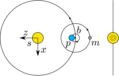
Figure 4: Sketch illustrating the orbital geometry of our edge–on planet–moon system at time $t=0$ as seen from the positive $y$–axis (left) and from the observer’s position at the positive $z$–axis (right). Indexes $s$, $p$, $m$, and $b$ refer to the positions of the star, the planet, the moon, and the planet–moon system barycenter, respectively. Distances and radii are not to scale.

Table 1 lists the orbital elements of our baseline planet–moon system. Both the barycenter’s and the lunar orbit are assumed to be circular ($e=0.0$), and their semi–major axes match those of the Earth–Moon system (Williams, 2017). We neglect the Earth–barycenter distance, so that $a_{\rm bs}=1$ AU. The semi–major axis of the lunar orbit, $a_{\rm mb}$, is computed from the Moon–Earth semi–major axis, $a_{\rm mp}=2.5696\cdot 10^{-3}$ AU (Williams, 2017), as follows:

$$a_{\rm mb}=a_{\rm mp}\hskip 1.42271pt\frac{m_{\rm p}}{m_{\rm p}+m_{\rm m}}\approx 2.54\cdot 10^{-3}\hskip 5.69046pt{\rm AU}\,,$$ (15)

with $m_{\rm p}$ and $m_{\rm m}$ the masses of the Earth and Moon, respectively. Because of the edge–on geometry, the right ascensions of the ascending nodes of the orbits of the barycenter and the moon are set to zero. Because both orbits are assumed to be circular, their perihelions are undefined. The barycenter’s argument of perihelion is chosen precisely behind the star at time $t=t_{0}=0$, i.e. $\omega_{\rm b}=270\degr$. For the moon, $\omega_{\rm m}$ is set to zero. The observational and orbital geometry at $t=0$ is sketched in Fig. 4. We use $R_{\rm p}=6371.0$ km and $R_{\rm m}=1737.4$ km for the baseline radii of the planet and the moon, respectively.

	Barycenter	Moon
$a$  [AU]	1.0	0.00254
$e$  [-]	0.0	0.0
$i$   [°]	90.0	0.0
$\omega$ [°]	270.0	0.0
$\Omega$ [°]	0.0	0.0
$t_{0}$ [sec]	0.0	0.0

Table 1: The orbital elements of the barycenter of our planet–moon system and of the orbit of the moon, with $a$ the semi–major axis, $e$ the eccentricity, $i$ the inclination angle, $\omega$ the argument of the perihelion, $\Omega$ the right ascension of the ascending node, and $t_{0}$ the time of perihelion passage. The inclination angle of the lunar orbit is defined with respect to the normal on the barycenter orbit.

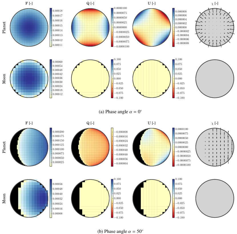
Figure 5: Reflected fluxes $F$, $Q$, and $U$, and the direction of polarization $\chi$ across the planet and the moon at $\alpha=0\degr$ (top) and 50$\degr$ (bottom). Fluxes $Q$ and $U$, and $\chi$ are defined with respect to the scattering planes of the planet and the moon, respectively. In order to facilitate the interpretation of the degree of polarization, we plot $180\degr-\chi$. Fluxes $Q$ and $U$ are zero across the moon’s disk because of the Lambertian reflection. All fluxes have been normalized such that the disk–integrated flux $F$ at $\alpha=0\degr$ equals the body’s geometric albedo. Absolute planetary fluxes per pixel are not comparable to the absolute lunar fluxes per pixel because of the different number of pixels across each disk.

3 Numerical results

Here, we present the computed total flux $F$, the linearly polarized fluxes $Q$ and $U$, and degree of polarization $P$ of starlight that is reflected by our model planet–moon system across time. As a trade–off between spatial resolution, radiometric and polarimetric accuracy, and computational time, we use 50 and 14 pixels along the equators of the planet and moon, respectively (see App. C), resulting in $N_{\rm p}=1956$ and $N_{\rm m}=156$ (Eq. 6). In Sect. 3.1, we analyze the individual contributions of the planet and the moon, and in Sect. 3.2, the results for the spatially unresolved planet–moon system. In Sect. 3.3, we take a closer look at particular transit and eclipse events.

3.1 Reflection by the spatially resolved planet & moon

In order to understand the traces of eclipses and transits in the flux and polarization of starlight reflected by spatially unresolved planet–moon systems, we first discuss the disk–resolved signals of the planet and the moon separately. Figure 5 shows the elements of the locally reflected Stokes vectors $\mathbf{F}^{\rm p}$ and $\mathbf{F}^{\rm m}$ and the direction of polarization $\chi$, with respect to the planetary and lunar scattering planes, respectively, at phase angles $\alpha$ of 0$\degr$ and 50$\degr$.

At $\alpha=0\degr$ (Fig. 5a), both the planet and the moon would be behind the star and thus invisible, but their disk–resolved signals give insight in the reflection processes. For both bodies, total flux $F$ is maximum at the sub-stellar/sub-observer region and decreases towards the terminator (which coincides with the limb at this phase angle). Because of the Lambertian reflection of the lunar surface and the lack of atmosphere around the moon, the reflected flux is unpolarized and $\chi$ undefined for the moon. The linearly polarized fluxes $Q$ and $U$ of the planet are due to Rayleigh scattering in the planet’s atmosphere. At the sub-stellar region, both $Q$ and $U$ are zero because of symmetry. The general increase of $Q$ and $U$ towards the limb is due to polarized second order scattered light, which is also apparent from the direction of polarization $\chi$. Because of its definition, $Q$ ($U$) equals zero along the lines at angles of 45^∘ (0^∘) and -45^∘ (90^∘) with the horizontal. Integrated across the planetary disk, $P$ would equal zero. Note that because of the Lambertian reflection of the surface of the planet, $Q$ and $U$ are independent of planetary surface albedo $a_{\rm surf}$, while $P$ will generally decrease with increasing $a_{\rm surf}$ because of the increasing flux $F$ (see e.g. Stam, 2008, for sample computations).

At $\alpha=50^{\circ}$ (Fig. 5b), the total flux $F$ of the moon is maximum at the sub-stellar region and decreases towards the terminator, due to the isotropic surface reflection and the absence of an atmosphere. The planet also shows a decrease of $F$ towards the terminator, but the location of the flux maximum is more diffuse and more towards the limb than on the moon, because light that is incident on the planet is scattered in the atmosphere in addition to being reflected by the surface; the reflected flux thus also depends on the optical path–lengths through the atmosphere, which in turn depend on the local illumination and viewing angles. The planet’s polarized fluxes $Q$ and $U$, and angle $\chi$ are mostly determined by starlight that has been singly scattered by the atmospheric gas molecules. For our choice of reference plane, $U$ is anti–symmetric with respect to this plane (and $U$ would thus equal zero when integrated across the disk), and $Q$ is symmetric. The negative values for $Q$ in Fig. 5b indicate that the reflected light is polarized perpendicular to the reference plane, which is indeed also clear from the polarization angle $\chi$, and what is expected for a Rayleigh scattering atmosphere.

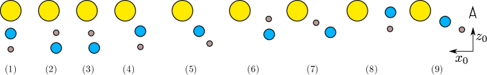
Figure 6: Sketch illustrating the sequence of planetary (1, 4, 8, …) and lunar (2, 6, …) transits, as well as planetary (3, 7, …) and lunar (1, 5, 9, …) eclipses for part of the barycenter’s orbit for an edge-on system. The positive $z_{0}$–axis points towards the observer. Position 1 corresponds to phase angle $\alpha=0^{\circ}$ and time $t=0$ s in our simulation (cf. Fig. 7).

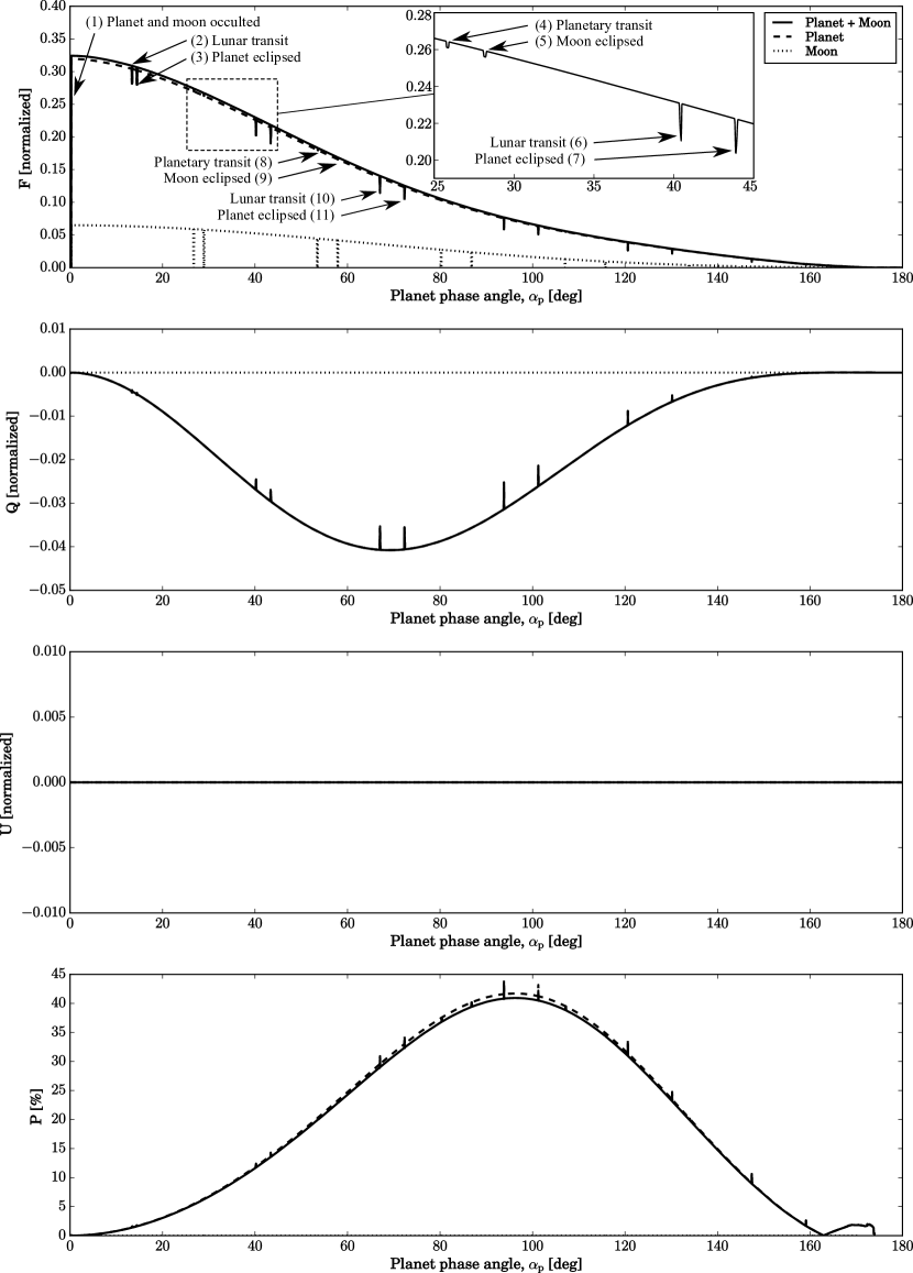
Figure 7: The total flux $F$, the linearly polarized fluxes $Q$ and $U$, and the degree of polarization $P$ of the spatially unresolved, edge–on, base-line planet–moon system, as functions of the planet’s phase angle $\alpha_{\rm p}$. Also included are curves for the isolated planet (coinciding with $Q$ and $U$ of the planet–moon system) and the isolated moon (equal to zero in $Q$, $U$, and $P$). Fluxes have been normalized such that at $\alpha_{\rm p}=0\degr$, $F$ equals the geometric albedo of the planet–moon system or each of the isolated bodies. The labels in the plot for $F$ refer to the illustrations in Fig. 6.

3.2 Reflection by the spatially unresolved planet & moon

Figure 7 shows the disk–integrated $F$, $Q$, $U$, and $P$ as functions of the planetary phase angle $\alpha_{\rm p}$. For our edge–on system, the curves cover only half of the barycenter’s orbital period. For comparison, we have also included curves for the planet and the moon as isolated bodies, thus without any mutual events. The total flux of the planet–moon system is lower than the sum of the total fluxes of the isolated planet and moon because the latter have not been scaled to the actual radii of the planet and the moon. Indeed the moon’s flux at $\alpha_{\rm p}=0^{\circ}$, equals the moon’s geometric albedo, i.e. 0.067, which matches the theoretical geometric albedo of a Lambertian reflecting body with surface albedo of 0.1 (see Stam et al., 2006). The geometric albedo of the unresolved planet–moon system (with both bodies at $\alpha_{\rm p}=0^{\circ}$ and next to each other) is about 0.33. Note that in Fig. 7, the observable planet–moon flux at $\alpha_{\rm p}=0^{\circ}$ is zero, because both bodies are then located behind the star as seen from the observer (in addition, the moon is located behind the planet, as can be seen from Fig. 4, and from situation 1 in Fig. 6).

The curves for $F$ decrease smoothly with increasing $\alpha_{\rm p}$, apart from the occasional sharp dips due to eclipses and transits (to be discussed below) and reach zero close to $\alpha_{\rm p}=180^{\circ}$, where the planet and moon would both be in front of the star. The slightly different slope of the lunar flux phase function as compared to that of the planet is due to the scattering of light in the latter’s atmosphere. As can be seen in Fig. 7, without the sharp dips, the smooth flux phase function of the planet–moon system does not reveal the presence of a moon, especially not without accurate information on the planetary radius, orbital distance, atmospheric and surface properties.

Because the lunar surface is completely depolarizing, the moon’s polarized fluxes $Q$ and $U$ are zero at each $\alpha_{\rm p}$. The disk–integrated $U$ of the light reflected by the planet is zero due to symmetry (see Fig. 5). Polarized flux $Q$ and degree of polarization $P$ of this light both show a smooth dependence on $\alpha_{\rm p}$, apart from the occasional sharp peaks that will be discussed below. The degree of polarization is maximum at phase angles between 90^∘ and 100^∘ due to the atmospheric Rayleigh scattering. At about 165^∘, the direction of polarization changes from perpendicular ($\chi=90^{\circ}$) to parallel ($\chi=0^{\circ}$) to the reference plane, and $P$ equals zero. The degree of polarization of the unresolved planet–moon system is somewhat lower than that of the isolated planet, because of the added unpolarized lunar flux. If the planetary atmosphere would contain clouds, the shape of this continuum curve would depend on the optical thickness and altitude of the clouds, the microphysical properties of the particles, and the cloud coverage across the planetary disk (for sample curves, see Rossi & Stam, 2017; Karalidi et al., 2012, and references therein).

While the smooth curves for the spatially unresolved planet–moon system shown in Fig. 7, do not provide direct evidence of the presence of a moon, the mutual events result in a series of dips and peaks in the reflected flux and polarization, respectively. Figure 6 illustrates the various events. Both the planet and the moon are initially ($\alpha_{\rm p}=0^{\circ}$) behind the star (position 1 in Fig. 6). Given the prograde lunar motion, the next event, when planet and moon are in view of the observer, is a lunar transit (position 2) and an eclipse of the star on the planet (3). After the first lunar period, the moon again disappears behind the planet (4), followed by an eclipse of the star on the moon (5). This sequence repeats along the barycenter’s orbit.

Both the planetary and lunar eclipses and transits temporarily reduce the flux $F$ that the observer receives. Indeed, when the planet transits the moon, the system’s flux phase function equals that of the isolated planet. The dip in the system’s flux due to a lunar transit (moon in front of the planet) will depend on the radius of the moon as compared to that of the planet and on the lunar surface albedo: the lower the lunar surface albedo and/or the larger the lunar radius, the deeper the dip compared to the continuum. The depth of the dip in the system’s flux $F$ due to an eclipse depends on the relative sizes of the moon and the planet, the reflection properties of the eclipsed body, and on the precise orbital geometry, especially because an eclipse shadow on the moon will not be completely black (cf. Fig. 2) (and the total flux $F$ thus slightly larger) due to starlight that is refracted through the limb of the planetary atmosphere and reaches the moon. This refraction is not included in our code (due to the wavelength dependence of Rayleigh scattering, the contribution of refracted light would be larger in the (near) infrared region of the spectrum than at 450 nm).

Because the moon reflects unpolarized light, neither a planetary transit (planet in front of the moon) nor an eclipse on the moon leads to a reduction of the polarized fluxes, as can be seen in Fig. 7. Because the planet reflects polarized light, a transit of the moon and an eclipse on the planet will both decrease $Q$ (given the geometry of our system). Because $P$ depends on $F$ and $Q$, the dips in $F$ due to less (unpolarized) lunar light being observed yield peaks in $P$. The peak value of $P$ that is due to the planet transiting the moon equals $P$ of the isolated planet at that value of $\alpha_{\rm p}$. In our computational results, peaks in $P$ that are due to an eclipse on the moon, would equal $P$ of the isolated planet when the whole lunar disk would be in the planet’s umbra because we neglect refracted starlight through the limb of the planetary atmosphere. Changes in $P$ that are due to the moon transiting the planet or due to the moon casting a shadow on the planet will depend on the total and polarized fluxes of the region of the planetary disk that is covered or darkened, and thus, for a given model planet and its atmosphere, on the relative sizes of the moon and the planet and the precise orbital geometry. This will be discussed further in Sect. 3.3.

The absolute depth of the dips in $F$ and $Q$ decreases with increasing $\alpha_{\rm p}$ because the fraction of a body’s disk that is illuminated and visible decreases with increasing $\alpha_{\rm p}$. The amplitudes of features in $P$ for our planet-moon model system are maximum when $\alpha_{\rm p}\approx 90\degr$. This is particularly convenient for exomoon detection with direct imaging techniques, because that is the phase angle range where the angular distance between the planet–moon system and the parent star will be largest.

As can be seen in Fig. 7, the phase angle gap between a lunar transit and the subsequent planetary eclipse (or a planetary transit and a subsequent lunar eclipse) increases with increasing $\alpha_{\rm p}$. As the orbital speed of both bodies is constant in our baseline system with circular orbits, this also applies in the time domain. Indeed, the lunar and planetary transits have a characteristic period because an observer–planet–moon alignment occurs twice per lunar orbit (see Fig. 6). The time gap between two consecutive transits and eclipses, however, increases with increasing $\alpha_{\rm p}$ because of the movement of the barycenter along its orbit.

3.3 Analysis of the mutual events

In this section, we analyze individual mutual events, i.e. their shape, symmetry, periodicity, magnitude, and duration. For this analysis, the change in flux $F$ and degree of polarization $P$ during an event are defined as follows

$$\Delta F = F_{\rm event}-F_{\rm continuum},$$ (16)

$$\Delta P = P_{\rm event}-P_{\rm continuum}.$$ (17)

First, we’ll discuss the lunar and planetary transits, then the lunar and planetary eclipses.

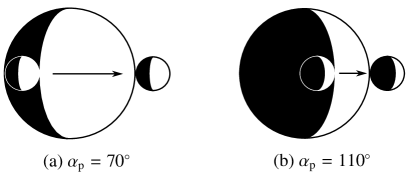
Figure 8: Sketch of the ingress and egress of the moon during a lunar transit for $\alpha_{\rm p}=70\degr$ and $\alpha_{\rm p}=110\degr$. The arrow indicates the direction of motion of the moon across the planetary disk.

Lunar transits

Figures 9a sand b provide detailed views of $\Delta F$ and $\Delta P$ during the six lunar transits (moon in front of the planet) shown in Fig. 7, together with sketches of the geometry of the planet and the moon at the beginning and the end of the transit for $\alpha_{\rm p}\approx 80^{\circ}$. As expected with constant orbital speeds, the duration of a lunar transit event decreases with increasing $\alpha_{\rm p}$ because of the decrease of the illuminated area on the planetary disk, and thus the shift of the time of ingress (see Fig. 8). Because egress takes place over the planetary limb, all curves in Figs. 9a and b have the same egress time. Also, the planet is relatively dark near the terminator, and thus yields a smooth flux decrease upon the lunar ingress, while it is bright near the limb (see Fig. 5), yielding a rapid increase of $F$ upon the lunar egress.

The depth $\Delta F$ depends strongly on $\alpha_{\rm p}$, because with increasing $\alpha_{\rm p}$, the illuminated area, and hence also the covered area on the planet decreases. The shape of $\Delta F$ also depends on $\alpha_{\rm p}$. At $\alpha_{\rm p}=0^{\circ}$, the curve would be symmetric. At larger values of $\alpha_{\rm p}$, the trace of the lunar night–side starts to appear in the curve. Because of the moon’s prograde orbit, the lunar day–side ingresses before the night–side. In the curves for $\alpha_{\rm p}=13.4^{\circ}$, and 40.3^∘, the steeper decrease of $F$ due to the ingress of the lunar night–side can be seen. The value of $\Delta F$ that is reached within a transit at a given $\alpha_{\rm p}$ depends on the lunar albedo and on the area of the planetary disk that is covered, thus on the lunar radius. The lower the lunar surface albedo and/or the larger the lunar radius as compared to the planetary radius, the larger $\Delta F$ will be. As an example, Fig. 11a shows $F$ at $\alpha_{\rm p}=67.2^{\circ}$ for various values of the lunar radius expressed as fraction of the planetary radius (the value for the baseline model is approximately 0.3). As can be seen, the continuum flux increases with increasing lunar radius due to the increased amount of flux reflected by the moon, and, indeed the lowest flux during the transit decreases and $\Delta F$ increases with increasing lunar radius.

Note that a change in the lunar radius implies a change in the lunar mass (assuming a similar composition) and, thus, a change in the lunar period around the planet. While the frequency of the events decreases non–linearly with increasing lunar radii, we have aligned the mutual events in Fig. 11 in time to facilitate a comparison. Mutual transits show up every half lunar sidereal period. Because $T\propto\sqrt{1/(M_{\rm m}+M_{\rm p})}$, relative timing variations of 1% to 13% are obtained for lunar–to–planet radius ratios from 0.1 to 0.7 (with our baseline value of approximately 0.3). In the case of eclipses, and assuming coplanar circular lunar and planetary orbits, the repetition period equals the lunar synodic period, for which timing variations of 1% to 14% are obtained for the same range of radii ratios.

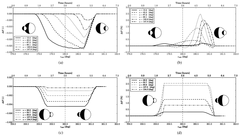
Figure 9: Changes in the total reflected flux $\Delta F$ (a and c), and the degree of polarization $\Delta P$ (b and d), as functions of the lunar true anomaly, $\nu_{\rm mb}$, and relative time for the lunar transits (top) and planetary transits (bottom) shown in Fig. 7. The time–step of these simulations is 3 minutes.

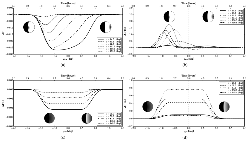
Figure 10: Similar to Fig. 9, except for the planetary eclipses (top) and the lunar eclipses (bottom), both as functions of angle $\varphi_{\rm ms}$ (see Fig. 12).

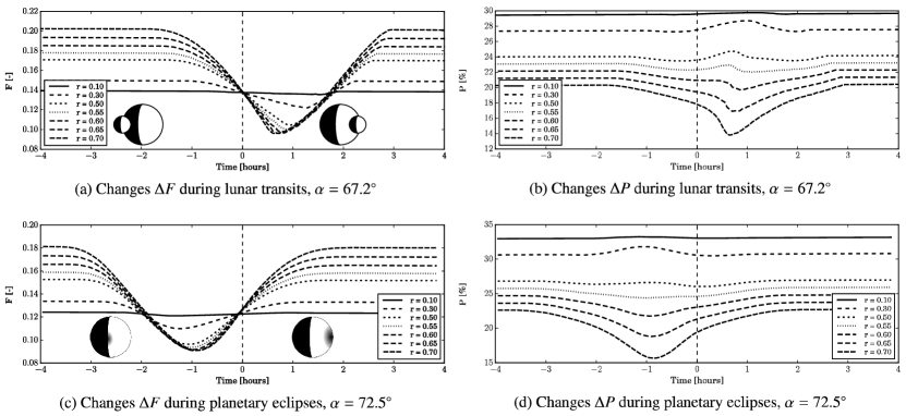
Figure 11: Changes in the total reflected flux $\Delta F$ (a and c) and $\Delta P$ (b and d) during lunar transits at $\alpha=67.2\degr$ (top) and planetary eclipses at $\alpha=72.5\degr$ (bottom) for various lunar–to–planetary radius ratios $r$. The horizontal axis shows the elapsed time since the concentric alignment of the planet and moon as seen from the star in the case of an eclipse and as seen from the observer in the case of a transit. The time–step of these simulations is 3 minutes. The baseline lunar–to–planetary radius ratio $r$ is about 0.3.

Figure 9b shows $\Delta P$ during lunar transits. It can be seen that $P$ can also decrease during a transit, which is not apparent from the curves in Fig. 7. The curves exhibit a strong variation in shapes, and with increasing $\alpha_{\rm p}$, get increasingly asymmetric. The largest $\Delta P$ is found around $\alpha_{\rm p}=90^{\circ}$, where $P$ of our model planet is highest (see Fig. 7). The precise shapes of the curves depend on the properties of the planet and its moon and the path of the transit across the planetary disk.

In our planet–moon system, the lunar transit occurs along the planet’s equator, where the antisymmetry of $U$ yields a null net contribution, and the shape of $\Delta P$ thus depends on the variation of $Q$ and $F$ along the path (cf. Fig. 5). At $\alpha_{\rm p}=13.4^{\circ}$, $Q$ is maximum near the planet’s limb and close to zero at the center of the body. The disk–integrated $P$ is close to zero due to symmetry. During ingress and egress, the moon breaks the symmetry, and (slightly) increases the disk–integrated value of $P$ (see Fig. 9b). With increasing $\alpha_{\rm p}$, the maximum $\Delta P$ increases, to reach a maximum (in the figure) at $\alpha_{\rm p}=90.1^{\circ}$. The $\alpha_{\rm p}$ where the maximum $P$ is found, corresponds roughly with the $\alpha_{\rm p}$ of the minimum $F$. This increase in $P$ appears to be driven by the decrease of $F$.

The negative values of $\Delta P$ in the curves for $\alpha_{\rm p}=67.2^{\circ}$, $90.1^{\circ}$ and 120.9^∘, indicate that during that part of the transit, the decrease in $Q$ is larger than that in $F$. This happens in particular when the illuminated part of the moon is transiting the illuminated part of the planetary disk, while the dark part of the moon is still transiting the dark part of the planet, and when the moon transits the limb of the planet, where $Q$ is relatively large and where the transit thus strongly decreases $Q$.

As mentioned earlier, the maximum $\Delta P$ (on the order of 2 % for our planet–moon system) should be observable when $\alpha_{\rm p}$ is between about 70^∘ and 150^∘, where the angular distance between the planet–moon and the star is relatively large, which would facilitate the detection of lunar transits with direct detection methods.

Figure 11b shows the change in $P$ at $\alpha_{\rm p}=67.2^{\circ}$, for various values of $r$, the lunar radius expressed as a fraction of the planetary radius. With increasing $r$, the continuum $P$ decreases because more unpolarized flux reflected by the moon is added to the total flux. During a transit, $P$ can be seen to be very sensitive to the lunar radius. Indeed, with increasing $r$, $\Delta P$ changes from positive ($P$ during the event is higher than in the continuum) to negative ($P$ during the event is lower than in the continuum) because apparently, the polarized flux reflected by the planet decreases more during the event than the total flux reflected by the planet with the moon in front of it.

Planetary transits

Figures 9c and d show the planetary transits (planet in front of the moon) from Fig. 7 in detail, both for $F$ and $P$. At $\alpha_{\rm p}=0^{\circ}$, the planet and the moon are behind the star and would thus not be visible to the observer, but, similarly to the lunar transits, planetary transits would yield symmetric events in $\Delta F$ and $\Delta P$. With increasing $\alpha_{\rm p}$, the events become more asymmetric.

With a planetary transit, the shapes of the $\Delta F$ curves are very different from those of the lunar transits, because, for our orbital geometry, the moon will be completely covered during the planetary transit and while it is covered, the transit curve is flat. The depth of the transit depends on the total amount of reflected flux received from the (isolated) moon. For a given value of $\alpha_{\rm p}$, $\Delta F$ will increase linearly with the surface area of the lunar disk (thus, with the lunar radius squared), and/or with the lunar surface albedo. The start time of the transit depends on $\alpha_{\rm p}$, as $\alpha_{\rm p}$ determines the extent of the illuminated area on the moon, and thus when it will be covered. Like with the lunar transits, the end of the transit, over the bright limb of the moon, is independent of $\alpha_{\rm p}$; it only depends on the lunar true anomaly.

For the planetary transits, $\Delta P$ is entirely due to the decrease in $F$, as the moon itself reflects only unpolarized light, and the planet thus blocks no polarized flux. As a result, the transits in $\Delta P$ are flat as long as the illuminated part of the lunar disk is covered. The maximum $\Delta P$ depends both on the $\Delta F$ and on the planet’s polarized flux $Q$, and thus on $\alpha_{\rm p}$ for a given planet-moon model. In Fig. 9d, a maximum $\Delta P$ of about 2.5$\leavevmode\nobreak\ \%$ occurs at $\alpha_{\rm p}=80.6\degr$. Through $\Delta F$, $\Delta P$ will increase with the lunar surface albedo and/or the surface area of the lunar disk at a given $\alpha_{\rm p}$ and for a given planet-moon model; a darker and/or smaller moon would yield a smaller $\Delta F$ and hence a smaller $\Delta P$.

Planetary eclipses

Figures 10a and b show the curves of $\Delta F$ and $\Delta P$ during the planetary eclipse events shown before in Fig. 7. During these eclipses, the moon casts its shadow on the planet, and because in our geometry the lunar orbital plane coincides with the barycenter’s orbital plane, the shadow of the moon travels along the horizontal line crossing the center of the planetary disk. Figure 12 illustrates the geometries for the planetary eclipse, with $\varphi_{\rm ms}$ the angle between the star and the moon measured positive in the counter clock–wise direction from the center of the planet. Angle $\varphi_{\rm ms}$ is used as relative measure of eclipse events. Its relation with time is linear, given the circular orbital motion of the bodies.

For planetary eclipses, the explanation regarding the asymmetry of $\Delta F$ and $\Delta P$ is the same as for lunar transits, with one important difference: while the transit events start increasingly later with increasing $\alpha_{\rm p}$ and end at the same (relative) time, the planetary eclipses start at the same (relative) time and end increasingly earlier with increasing $\alpha_{\rm p}$. The reason for this difference is that eclipses depend on the position of the star with respect to the planet–moon system, and not on the position of the observer. The observer’s position does influence the fraction of the eclipse that is captured, as it determines the phase angle and hence the fraction of the illuminated part of the planetary disk across which the eclipse travels. Thus, with increasing $\alpha_{\rm p}$, the duration of an eclipse decreases, as is visible in Figs. 10a and b. The depth $\Delta F$ decreases with increasing $\alpha_{\rm p}$ because less of the illuminated part of the planetary disk is visible.

The shape of the $\Delta F$ curves for the planetary eclipses (where the moon’s shadow moves across the planetary disk) appears to be more gradual than that of the lunar transit curves (where the moon itself moves across the planetary disk) (cf. Fig. 9). This is because the planet first travels through the lunar penumbral shadow, before entering the deep, umbral shadow cone. Because we discuss only half of the barycenter’s orbit, the ingress of the lunar eclipse shadow on the illuminated part of the planetary disk is through the terminator and the egress through the bright limb, as illustrated in Figs. 8 and 12. However, because the spatial extent of the penumbral and umbral shadows across the disk are smallest halfway the total duration of the eclipse (as seen from a vantage point on the moon facing the planet), the egress of the lunar shadow yields a much smoother $\Delta F$ curve than observed during the egress of a lunar transit. The difference in the maximum $\Delta F$ during a lunar transit and a planetary eclipse is most apparent at the smaller phase angles, because with increasing $\alpha_{\rm p}$, the contribution of light reflected by the moon decreases. Note that differently than for lunar transits, the value of $\Delta F$ during a planetary eclipse is independent of the lunar surface albedo. It will obviously increase with the radius of the moon relative to that of the planet. This can also be seen in Figs. 11c and d, which show $F$ at $\alpha_{\rm p}=72.5^{\circ}$ for various values of $r$, the lunar radius expressed as fraction of the planetary radius (for the baseline model, $r$ is 0.3). Indeed, with increasing $r$, the continuum flux increases because of the added flux reflected by the moon, and the minimum flux during the event decreases because of the increasing extent of the lunar shadow.

The change in $P$ during the planetary eclipses is shown in Fig. 10b. The increase in $P$ during the ingress of the lunar shadow is due to the decrease in $F$ and a decrease in $Q$. As the shadow progresses across the disk, its spatial extent decreases, and its influence on $P$ decreases. The maximum of $\Delta P$ appears to be $1-2\leavevmode\nobreak\ \%$ for phase angles $\alpha_{\rm p}\approx 70\degr-160\degr$. For the largest phase angles, the corresponding value of $\Delta F$ is relatively small, because only a narrow crescent of the planet is illuminated, so there $\Delta P$ is mostly due to a change in $Q$.

Figure 11d shows $P$ at $\alpha_{\rm p}=72.5^{\circ}$ for various values of $r$ (the lunar radius expressed as fraction of the planetary radius). With increasing $r$, the continuum $P$ decreases because of the added unpolarized flux reflected by the moon, and $P$ during the eclipse decreases, too, apparently because the polarized flux $Q$ decreases more than the total flux $F$.

Figure 12: The geometrical definition of angle $\varphi_{\rm ms}$ as moon $m$ passes between planet $p$ and star $s$. Seen from the top, the moon moves anti–clockwise around the planet. A similar definition holds for angle $\varphi_{\rm mp}$ as the planet passes between the moon and the star. Distances between bodies and radii are not to scale.

Lunar eclipses

As can be seen in Figs. 10c and d, lunar eclipses, when the planet casts its shadow on the moon, show a similar symmetry as the planetary transits, where the planet moves in front of the moon (Fig. 9c and d). Because our model moon is small compared to the planetary shadow, both the $\Delta F$ and $\Delta P$ curves are flat except during ingress and egress. The flux changes during ingress and egress of the lunar eclipse, respectively, are smoother than with the planetary transits, due to the extended penumbral region of the planet’s shadow.

Like with the planetary eclipses discussed above, the moon’s ingress into the planetary shadow occurs at the same value of angle $\varphi_{\rm ms}$ (cf. Fig. 12) independent of phase angle $\alpha_{\rm p}$. The duration of the eclipse decreases with increasing $\alpha_{\rm p}$ because of the decrease of the illuminated area on the moon with increasing $\alpha_{\rm p}$. The change in $P$ during lunar eclipses, shown in Fig. 10, is similar to that during planetary transits (Fig. 9), as in both cases $P$ changes during the event because $F$ decreases and because there is no actual change in the amount of polarized flux from the system, because our model moon reflects only unpolarized light. The maximum $\Delta P$ value is about $2.7\leavevmode\nobreak\ \%$, attained at $\alpha_{\rm p}\approx 87.1^{\circ}$ in Fig. 10.

With increasing lunar radius as compared to the planetary radius, and depending on the distance between the moon and the planet and the distance to the star, the planetary shadow might cover only part of the lunar disk. In that case, $F$ and $P$ will no longer be flat during the eclipse, because there will be a contribution of unpolarized lunar flux that will vary in time. Indeed, the curves will become asymmetric (more similar to those for the planetary eclipses). Because the moon only reflects unpolarized flux, $P$ will always increase during the eclipses.

4 Conclusions

We present numerically simulated flux and polarization phase functions of starlight that is reflected by an orbiting planet–moon system, including mutual events, such as transits and eclipses. Most results presented in this paper apply to a Moon–sized, Lambertian (i.e. isotropically and depolarizing) reflecting moon orbiting an Earth–sized exoplanet with an Earth–like, gaseous atmosphere on top of a Lambertian reflecting surface (the surface pressure is 1 bar), in an edge–on configuration. Our results show that the flux and polarization phase functions of starlight reflected by such a planet–moon system contain traces of the moon in the form of periodic changes in the total flux $F$ and degree of polarization $P$ as the bodies shadow each other (eclipses) and/or hide one another from the observer’s view (transits) along their orbit around the star. These changes in $F$ and $P$ are only one order of magnitude smaller than the system’s continuum phase functions. The magnitude, shape and duration of the obtained total flux signatures are comparable with the results by Cabrera & Schneider (2007), except that they do not include the influence of the penumbra.

During events that darken the planet, i.e. the lunar transits and planetary eclipses, the shape of the dip in $F$ depends on the reflection properties of the regions on the planet along the path of the shadow. The change in $P$ during such events strongly depends on the ratio of polarized–to–total reflected flux across the disk and along the path of the shadow. Indeed, $\Delta P\approx 1\%-1.8\%$ for $67\degr<\alpha_{\rm p}<121\degr$. For the planet–moon system used in this paper, we found the strongest changes in $P$ during either the first (planetary eclipse) or the last (lunar transit) half of the event, compared to the duration of the event in $F$, in particular at intermediate phase angles. The asymmetry of the planet darkening events as imprinted on the change in polarization $\Delta P$ is due to the variation of the polarization across the planetary disk with our model atmosphere–surface: the polarized flux at the limb is higher than at the terminator.

During lunar darkening events, i.e. planetary transits and lunar eclipses, the size difference between the planet and the moon yields a relatively symmetric change in $F$ and, due to the non–polarizing lunar reflection, a similarly relatively symmetric change in $P$, as the latter is only due to the decrease in total flux, upon a lunar darkening event, not to a change in polarized flux. The curves for planetary transits have steeper slopes during the ingress and egress phases than the curves for the lunar eclipses, because with the latter, the moon travels through the penumbral shadow of the planet. The change in $P$ depends on the size and albedo of the moon, and on the polarization signal of the planet, which itself depends on the atmosphere-surface model and the phase angle. Our simulations have been performed at 450 nm, i.e. in the blue, where the scattering by the gas in the Earth–like planetary atmosphere strongly contributes to the planet’s polarization signals. In particular at intermediate phase angles, the polarization signal of a gaseous atmosphere is strong, and the change in polarization during the lunar darkening events can reach a few percent. Indeed, $\Delta P\approx 1.25\%-2.66\%$ for $54\degr<\alpha_{\rm p}<108\degr$ during planetary transits. Note that at these phase angles, the angular distance between the planet–moon system and the parent star is relatively large, so these angles are favorable for the detection of reflected starlight. For a planet with clouds in its atmosphere, the continuum flux phase function will have a similar shape as that for our cloud–free planet, except the total amount of reflected flux will be larger (of course not at wavelengths where atmospheric gases absorb the light). The polarization curve of a cloudy planet will show angular features due to the scattering of light by the cloud particles, such as the rainbow for liquid water droplets (see e.g. Karalidi et al., 2012; Bailey, 2007, and references therein).

The duration of a transit event depends on the orbital parameters, on the sizes of the planet and moon, and on the phase angle (the latter mostly for lunar transits). In our simulations, a typical planetary transit takes $\sim 4$ hours both in flux and polarization. A lunar transit at an intermediate phase angle of 90^∘, takes about 2 hours in flux. In polarization, the change in $P$ is apparent during a shorter period than the change in flux $F$, due to the distribution of polarized flux across the planetary disk. The duration of eclipse events is somewhat longer than that of transit events due to the diverging shape of the shadow cone. In our simulations, eclipse events can take up to 6 hours, where the polarization change in the planetary eclipses is only apparent during part of the time of the flux change.

The results presented in this paper correspond to half of the planetary orbit around the star. The results for the other half of the orbit will be similar, except that the curves will be mirrored with respect to the central event time, because transit and eclipse ingresses and egresses will happen over the other side of the darkened body.

Our results show that measuring the temporal variation in $F$ and/or $P$ during transits and eclipses could provide extra information on the properties of a planet and/or moon and their orbits. Extracting such information, however, requires not only detecting such events but also measuring the shape of the variations in $F$ and/or $P$. For the interpretation of such measurements, numerical simulations to map in more detail the influence of the physical characteristics of the moon and the planet (radius, albedo, atmosphere-surface properties) and their orbital characteristics (inclination angles, ellipticity) on the temporal variation in $F$ and $P$ are required. Such simulations will be targeted in future research.

Appendix A Local illumination and viewing angles

In this appendix, we describe the computation of the angles required to compute the starlight that is reflected by each pixel on the planet (cf. Eq. 8): the phase angle $\alpha$, the local viewing zenith angle $\theta_{i}$, the local illumination zenith angle $\theta_{0i}$, the local azimuthal difference angle $\phi_{i}-\phi_{0i}$, and the local rotation angle $\beta_{i}$. To add the computed Stokes vectors of the moon to those of the planet, we usually also need rotation angle $\psi$ that redefines the lunar Stokes vector from the lunar scattering plane to the planetary scattering plane (cf. Eq. 4).

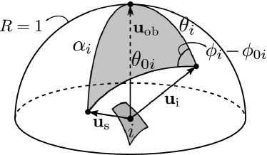
Figure 13: Angular geometry of the spherical triangle centered at pixel $i$ and defined by the zenith direction unit vector, $\mathbf{u}_{\rm zi}$, the observer’s direction unit vector, $\mathbf{u}_{\rm ob}$, and the star direction unit vector, $\mathbf{u}_{\rm s}$. The sides of the spherical triangle are: the observer–zenith angle $\theta_{i}$ , the star–zenith angle $\theta_{0i}$, and the pixel–based phase angle $\alpha_{i}$, all centered at pixel $i$. The angle between sides $\theta_{0i}$ and $\theta_{i}$ is the azimuthal difference angle $\phi_{i}-\phi_{0i}$.

A.1 Phase angle $\alpha_{\rm x}$

Phase angle $\alpha$ is the angle between the direction to the star and the observer, as measured from the center of a body (see Fig. 13). In principle its value ranges from 0^∘ to $180\degr$, although the phase angle range accessible to an observer depends on the inclination angle of the orbit of a body. A body in an edge–on orbital geometry (inclination angle $i=90^{\circ}$) can attain phase angles between 0^∘ (when it is located behind the star) and 180^∘, while a body in a face–on orbital geometry ($i=0^{\circ}$) can only be observed at $\alpha=90^{\circ}$. Generally, given an orbital inclination angle $i$, the phase angle range is given by

$$90^{\circ}-i\leq\alpha\leq 90^{\circ}+i.$$ (18)

The phase angle of the planet or the moon at time $t$ is computed as

$$\alpha_{\rm x}(t)=\arccos\left[\mathbf{u}^{T}_{\rm z}\cdot\left(-\frac{\mathbf{r}_{\rm xs}(t)}{\left\lVert\mathbf{r}_{\rm xs}(t)\right\rVert}\right)\right]\,,$$ (19)

where subscript ’x’ refers to either ’p’ (planet) or ’m’ (moon), $\mathbf{u}^{T}_{\rm z}=\left[0,0,1\right]$ is the unit vector along the $z$–axis, pointing towards the observer, and vector ${\bf r}_{\rm xs}$ connects the center of the planet or moon with the center of the star. Given the small separation between the planet and moon compared to their distances to the star, $\alpha_{\rm p}$ is virtually the same as $\alpha_{\rm m}$, yet our numerical model uses both values.

A.2 Local viewing zenith angle $\theta_{i}$

The local viewing zenith angle $\theta_{i}$ is the angle between the zenith direction of pixel $i$ and the direction towards the observer (see Fig. 13). Angle $\theta_{i}$ takes values between $0\degr$ (at the sub-observer location) and $90\degr$ (at the limb). It depends on the location of the pixel on the disk of the planet or moon and is thus time-independent. It is computed according to

$$\theta_{i}=\arccos\left[\mathbf{u}^{T}_{\rm z}\cdot\frac{\mathbf{r}_{i{\rm x}}}{\left\lVert\mathbf{r}_{i{\rm x}}\right\rVert}\right]\,,$$ (20)

where subscript ’x’ refers to either ’p’ or ’m’, $\mathbf{u}_{\rm z}$ is the unit vector along the $z$–axis that points towards the observer, and $\mathbf{r}_{i{\rm x}}$ is the vector pointing to the center of the pixel from the center of either the planet or the moon.

A.3 Local illumination zenith angle $\theta_{0i}$

The local illumination zenith angle $\theta_{0i}$ is defined as the angle between the local zenith direction of pixel $i$ and the direction towards the star (see Fig. 13). Angle $\theta_{0i}$ takes values between $0^{\circ}$ (at the sub-stellar location) and $90^{\circ}$ (at the terminator). The position of the star changes in time, so that the time–dependent local illumination zenith angle can be computed as

$$\theta_{0i}(t)=\arccos\left[\,\frac{\mathbf{r}^{T}_{i{\rm x}}(t)}{\left\lVert\mathbf{r}_{i{\rm x}}(t)\right\rVert}\cdot\left(-\frac{\mathbf{r}_{i{\rm s}}(t)}{\left\lVert\mathbf{r}_{i{\rm s}}(t)\right\rVert}\right)\right]\,,$$ (21)

where subscript ’x’ refers to either ’p’ or ’m’, $\mathbf{r}_{i{\rm x}}$ is the vector from the center of the planet or moon to the center of the pixel, and $\mathbf{r}_{i{\rm s}}$ the vector from the center of the star to the center of the pixel on the planet or moon.

A.4 Local azimuthal difference angle $\phi_{i}-\phi_{0i}$

The azimuthal difference angle $\phi_{i}-\phi_{0i}$ for pixel $i$ on the planet or moon is the angle between the plane described by the local zenith direction and the direction towards the observer and the plane described by the local zenith direction and the direction towards the star. As Fig. 13 shows, $\phi_{i}-\phi_{0i}$ follows from

$$\phi_{i}-\phi_{0i}(t)=\arccos{\left(\frac{\cos{\alpha_{i}(t)}-\cos{\theta_{i}}\cos{\theta_{0i}(t)}}{\sin{\theta_{i}}\cos{\theta_{0i}(t)}}\right)}\,.$$

where $\alpha_{i}$ is the angle between the direction to the observer and the direction to the star measured from the center of pixel $i$. Given that $\left\lVert\mathbf{r}_{i{\rm x}}\right\rVert\ll\left\lVert\mathbf{r}_{\rm xs}\right\rVert$ with ’x’ referring to either ’p’ or ’m’, $\alpha_{i}$ can be approximated by the body’s phase angle $\alpha_{\rm x}$, and thus

$$\phi_{i}-\phi_{0i}(t)=\arccos{\left(\frac{\cos{\alpha_{\rm p}(t)}-\cos{\theta_{i}}\cos{\theta_{0i}(t)}}{\sin{\theta_{i}}\cos{\theta_{0i}(t)}}\right)}\,.$$ (22)

A.5 Local rotation angle $\beta_{i}$

Angle $\beta_{i}$ is used to rotate a locally computed vector ${\bf F}^{\rm x}_{i}$ (see Eq. 6) for pixel $i$ on the planet or the moon from the local meridian plane to the scattering plane of the body, which is used as the reference plane for the disk–integrated signal of the body. The pixel grid across the planet is defined with respect to the planetary scattering plane, and $\beta_{i}$ is thus time independent for the planetary pixels. For a pixel $i$, $\beta_{i}$ is computed according to

$$\beta_{i}=\arcsin{\dfrac{y_{i{\rm p}}}{x^{2}_{i{\rm p}}+y^{2}_{i{\rm p}}}}\,,$$ (23)

where $x_{i{\rm p}}$ and $y_{i{\rm p}}$ are the coordinates of the center of the pixel (recall that the $z$–axis points towards the observer).

For the lunar pixels, the alignment between the lunar scattering plane and the lunar grid, and hence angle $\beta_{i}$, is time-dependent and requires to redefine the pixel coordinates with respect to the lunar scattering plane. Indicating the redefined coordinates of lunar pixel $i$ with subscript $j$, angle $\beta_{j}$ is then computed as:

$$\beta_{j}(t)=\arcsin{\frac{y_{j{\rm m}}(t)}{x^{2}_{j{\rm m}}(t)+y^{2}_{j{\rm m}}(t)}}.$$ (24)

A.6 Scattering plane rotation angle $\psi$

Scattering plane rotation angle $\psi$ is used to rotate a Stokes vector that is defined with respect to the lunar scattering plane to the planetary scattering plane, which we use as the reference plane for the planet–moon system. Angle $\psi$ is measured in the clock–wise direction from the lunar scattering plane to the planetary scattering plane. For the results presented in this paper, the moon and the planet orbit in the same, edge–on plane, and angle $\psi$ equals zero. In the general case, however, it is computed using

$$\psi(t)=\arctan\left(-(\mathbf{u}^{T}_{\rm y}\cdot\mathbf{r}_{\rm ms}(t))/(\mathbf{u}^{T}_{\rm x}\cdot\mathbf{r}_{\rm ms}(t))\,\right)\,,$$ (25)

where $\mathbf{r}_{\rm ms}$ is the vector from the star to the center of the moon, and $\mathbf{u}_{\rm x}$ and $\mathbf{u}_{\rm y}$ are the unit vectors along the $x$-axis and $y$-axis in coordinate system $S_{1}$.

Appendix B Computing eclipses

An eclipse occurs when body $A$ is between the star $S$ and body $B$ such that the shadow of $A$ falls onto $B$. The effect of a planetary or lunar eclipse depends on the positions of the star, moon and planet, and, due to the extended size of the star, the size, shape, and depth of the shadow depend not only with the radii of the star and the eclipsing body, but also on the distances and angles involved. Computing eclipses has been discussed in great detail by Link (1969) for the Moon–Earth system, which we apply to our exoplanetary system. We model the umbral, antumbral, and penumbral shadow regions. Figure 14 shows the geometries involved in the various types of eclipses. The equations used for computing the influence of eclipses are described here.

The flux arriving at a pixel $i$ of eclipsed body $B$ at time $t$ depends on the fraction of the stellar disk and the local stellar surface brightness, as seen from the center of the pixel. In Eq. 6, this is accounted for by factor $c_{i}$, the ratio between the actual flux $e^{\prime}_{i}$ on pixel $i$ and $e_{i}$, the flux on the non–eclipsed pixel:

$$c_{i}(t)=e^{\prime}_{i}(t)/e_{i}(t)=S^{\prime}_{Si}(t)/S_{Si}(t),$$ (26)

with $S^{\prime}_{Si}$ and $S_{Si}$ the stellar disk area as observed from pixel $i$ when it is eclipsed and when it is non–eclipsed, respectively. Note that we ignore stellar limb darkening and stellar light that travels through the atmosphere of the eclipsing body (if present).

To determine $c_{i}$, we first have to identify whether or not pixel $i$ is eclipsed. Obviously, $c_{i}=1$ for a non–eclipsed pixel. If the pixel is (partly eclipsed), we have to determine the type of eclipse: umbral (i.e. total), antumbral, or annular. . For an umbral eclipse $c_{i}=0.0$, for an antumbral and annular eclipse, we have to compute $S^{\prime}_{Si}$ in order to determine $c_{i}$.

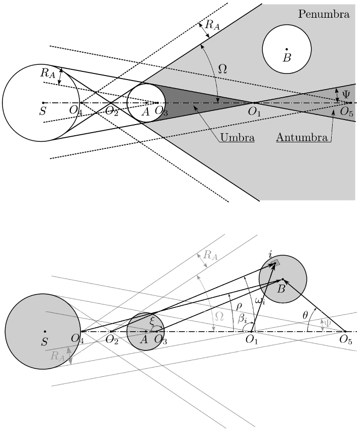
Figure 14: Geometry of the umbral, antumbral and penumbral shadow cones, when star $S$ is eclipsed by body $A$, casting a shadow on body $B$. The shadow casted by $A$ into space is rotationally symmetric around the axis through the center of the star and body $A$. The radii of the star, body $A$ and body $B$ are denoted by $R_{S}$, $R_{A}$, and $R_{B}$, respectively. Points $O_{1}$, $O_{2}$, $O_{3}$, $O_{4}$ and $O_{5}$ denote auxiliary points: the umbral and antumbral cones have apex $O_{1}$ and aperture $2\Psi$ and the penumbral cone has apex $O_{2}$ and aperture $2\Omega$. The lower figure also shows angles $\zeta$, $\rho$, $\omega_{i}$, $\beta_{i}$, and $\theta$, that are used in the computation of the eclipse shadow depth. Distances between bodies and radii are not to scale in order to emphasize the geometry of the system.

As can be seen in Fig. 14, a pixel on body $B$ is eclipsed when it falls within the penumbral cone of body $A$. Opening angle $\Omega$ of the penumbral cone is given by:

$$\sin{\Omega}=\dfrac{R_{S}+R_{A}}{\left\lVert\mathbf{r}_{\rm AS}\right\rVert}\,.$$ (27)

Indeed, pixels in eclipse on the disk of body $B$ can be found at times when

$$\sin{\rho}(t)<\sin{\Omega}(t),$$ (28)

with angle $\rho$ ($\left[0\degr,90\degr\right)$) given by (see Fig. 14)

$$\cos{\rho}=\dfrac{-\left(\mathbf{r}_{\rm AB}-\mathbf{AO_{4}}\right)\cdot\mathbf{u}_{\rm AS}}{\left\lVert\mathbf{r}_{\rm AB}-\mathbf{AO_{4}}\right\rVert}\,.$$ (29)

Vector $\mathbf{AO_{4}}$ is a function of the radii of the shadowed and eclipsing bodies and of $\Omega$, as follows:

$$\mathbf{AO_{4}}=\dfrac{R_{B}+R_{A}}{\sin{\Omega}}\,\mathbf{u}_{\rm AS}\,.$$ (30)

Except when body $B$ falls completely in the penumbral cone, there will also be non–eclipsed pixels on the disk. When Eq. 28 holds, a pixel-by-pixel search is performed, in which the center of each pixel is checked for total or umbral (Sect. B.1), annular (Sect. B.2), or penumbral (Sect. B.3) eclipse conditions.

B.1 Total or umbral eclipses

In the umbral zone (see Fig. 14), pixels experience a total stellar eclipse. If the umbral zonal is wide and the shadowed body $B$ relatively small, such as in the Earth–moon system, all pixels on the disk of $B$ can be simultaneously in the umbra, and factor $c_{i}=0$ for all pixels. This is the case when

$$\cos{\xi}>\cos{\Psi}\,,$$ (31)

with

$$\sin{\Psi}=\dfrac{R_{S}-R_{A}}{\left\lVert\mathbf{r}_{\rm AS}\right\rVert}\,,$$ (32)

and

$$\cos{\xi}=\frac{\left(\mathbf{r}_{\rm AB}-\mathbf{AO_{3}}\right)\cdot\mathbf{u}_{\rm AS}}{\left\lVert\mathbf{r}_{\rm AB}-\mathbf{AO_{3}}\right\rVert}\,\hskip 11.38092pt{\rm with}\hskip 11.38092pt\mathbf{AO_{3}}=-\dfrac{R_{A}-R_{B}}{\sin{\Psi}}\,\mathbf{u}_{\rm AS}\,.$$ (33)

The disk of body $B$ will only be partially inside the umbral shadow cone of body $A$ when

$$\cos{\Psi}<\dfrac{\left(\mathbf{r}_{\rm AB}-\mathbf{AO_{5}}\right)\cdot\mathbf{u}_{\rm AS}}{\left\lVert\mathbf{r}_{\rm AB}-\mathbf{AO_{5}}\right\rVert}$$ (34)

and

$$\left(\left\lVert\mathbf{O_{5}B}\right\rVert>\dfrac{R_{B}}{\tan{\Psi}}\hskip 8.5359pt\text{or}\hskip 8.5359pt\left\lVert\mathbf{O_{1}B}\right\rVert<R_{B}\right)$$ (35)

Here

$$\mathbf{O_{5}B}=\mathbf{r}_{\rm AB}-\mathbf{AO_{5}}\hskip 14.22636pt{\rm and}\hskip 14.22636pt\mathbf{O_{1}B}=\mathbf{r}_{\rm AB}-\mathbf{AO_{1}}\,,$$ (36)

with

$$\mathbf{AO_{5}}=-\dfrac{R_{B}+R_{A}}{\sin{\Psi}}\,\mathbf{u}_{\rm AS}\hskip 14.22636pt{\rm and}\hskip 14.22636pt\mathbf{AO_{1}}=-\dfrac{R_{A}}{\sin{\Psi}}\,\mathbf{u}_{\rm AS}\,.$$ (37)

If the disk of body $B$ falls partially inside the umbral cone, the pixels where $\beta_{i}<\Psi$ are inside the umbra, and $c_{i}=0$. Because $c_{i}$ only applies to pixels on the illuminated part of the disk of $B$, this condition can be reformulated as

$$\sin{\beta_{i}}<\sin{\Psi}\,.$$ (38)

Note that angle $\beta_{i}$ of a pixel can be derived from

$$\cos{\beta_{i}}=\dfrac{\left(\mathbf{r}_{\rm Ai}-\mathbf{AO_{1}}\right)\cdot\mathbf{u}_{\rm AS}}{\left\lVert\mathbf{r}_{\rm Ai}-\mathbf{AO_{1}}\right\rVert}\,.$$ (39)

The pixels on the disk of $B$ that are not in the umbral cone can be in the antumbral or annular eclipse zone, as described below.

B.2 Annular or antumbral eclipses

Instead of crossing the umbral cone, body $B$ can cross the antumbral cone, where eclipsing body $A$ does not completely cover the stellar disk as seen from body $B$, thus yielding a so–called annular eclipse. Body $B$ is in the antumbral shadow cone when

$$\cos{\xi}<-\cos{\Psi}\,,$$ (40)

where $\xi$ and $\Psi$ follow from Eqs. 33 and 32. When Eq. 40 is satisfied, pixels on the disk of $B$ are checked for their eclipsed status. A pixel is (partially) eclipsed if

$$\cos{\beta_{i}}<-\cos{\Psi}\,.$$ (41)

For each pixel in the antumbral cone, factor $c_{i}$ is given by the fraction of the stellar disk that is visible (see Fig. 15), i.e.

$$c_{i}=\dfrac{\pi\alpha^{2}_{Si}-\pi\alpha^{2}_{Ai}}{\pi\alpha^{2}_{Si}}=1-\left(\dfrac{\alpha_{Ai}}{\alpha_{Si}}\right)^{2}\,,$$ (42)

where

$$\alpha_{Si}=\arcsin{\dfrac{R_{Si}}{\left\lVert\mathbf{r}_{Si}\right\rVert}}\,\hskip 14.22636pt{\rm and}\hskip 14.22636pt\alpha_{Ai}=\arcsin{\dfrac{R_{Ai}}{\left\lVert\mathbf{r}_{Si}\right\rVert}}\,.$$ (43)

Here, $\mathbf{r}_{Si}$ is the position vector of pixel $i$ on body $B$ with respect to the center of star $S$.

Figure 15: The disks of star $S$ and eclipsing body $A$ seen from a pixel on body $B$ in the antumbral zone. Angles $\alpha_{S}$ and $\alpha_{A}$ indicate the angular radii of the bodies.

B.3 Penumbral eclipses

When Eq. 28 holds, all pixels that are not in the umbral or antumbral eclipse are examined for being in the penumbral shadow. Indeed, pixels with $\omega_{i}<\Omega$ are within the penumbral cone, as can be seen in Fig. 14. This inequality can be rewritten as

$$\cos{\omega_{i}}>\cos{\Psi}\,,$$ (44)

where $\cos{\Psi}$ follows from Eq. 32 and $\cos\omega_{i}$ is given by:

$$\cos{\omega_{i}}=\dfrac{-\left(\mathbf{r}_{\rm Ai}-\mathbf{AO_{2}}\right)\cdot\mathbf{u}_{\rm AS}}{\left\lVert\mathbf{r}_{\rm Ai}-\mathbf{AO_{2}}\right\rVert}\,\hskip 11.38092pt{\rm with}\hskip 11.38092pt\mathbf{AO_{2}}=\dfrac{R_{A}}{\sin{\Omega}}\,\mathbf{u}_{\rm AS}\,.$$ (45)

The magnitude of the eclipse at pixel $i$, $c_{i}$, can be calculated through the stellar and eclipsing body viewing angles, i.e. the angular diameter of the bodies, $2\alpha_{S}$ and $2\alpha_{A}$, and the eclipsing body-to-star angular distance as seen from the shadowed body, $\delta$. Then, as follows from Fig. 16, $c_{i}$ can be computed using

$$c_{i}=\dfrac{\pi\alpha_{S}^{2}-A_{1}-A_{2}}{\pi\alpha_{S}^{2}}=1-\dfrac{A_{1}+A_{2}}{\pi\alpha_{S}^{2}},$$ (46)

with

$$A_{1}=\left\{{\begin{array}[]{*{20}{l}}\dfrac{\theta_{A}-\sin{\theta_{A}}}{2}\hskip 2.84544pt\alpha_{A}^{2}\hskip 28.45274pt\text{if}\hskip 5.69046pt\delta\geq l_{S}\\ \\ \pi-\dfrac{\theta_{A}-\sin{\theta_{A}}}{2}\hskip 2.84544pt\alpha_{A}^{2}\hskip 12.80365pt\text{if}\hskip 5.69046pt\delta<l_{S}\end{array}}\right.\,$$ (47)

and

$$A_{2}=\left\{{\begin{array}[]{*{20}{l}}\dfrac{\theta_{S}-\sin{\theta_{S}}}{2}\hskip 2.84544pt\alpha_{S}^{2}\hskip 28.45274pt\text{if}\hskip 5.69046pt\delta\geq l_{A}\\ \\ \pi-\dfrac{\theta_{S}-\sin{\theta_{S}}}{2}\hskip 2.84544pt\alpha_{S}^{2}\hskip 12.80365pt\text{if}\hskip 5.69046pt\delta<l_{A}\end{array}}\right.\,$$ (48)

Figure 16: Stellar ($S$) and eclipsing body ($A$) disks as seen from a pixel on the shadowed body during a penumbral eclipse. The stellar shadowed area is decomposed in two components $A_{1}$ and $A_{2}$. $\alpha_{S}$ and $\alpha_{A}$ stand for the angular radius of the bodies, and $\delta$ is the angular separation between the bodies’ center. $\theta_{S}$ and $\theta_{A}$ are the central angles of the circular segments defined by the common cord of the intersecting stellar and eclipsing body disks. The minimum distance from the star/eclipsing body center to the common chord is defined as $l_{S}$/$l_{A}$.

Here, $l_{S}$ and $l_{A}$ are the distances from the centers of the stellar disk and eclipsing body $A$, respectively, to the line between the two points where the stellar and eclipsing body intersect. The angles $\theta_{S}$ and $\theta_{A}$ (see Fig. 16) follow from e.g. Heron’s formula:

$$\theta_{S}=2\arcsin{\left(\dfrac{2}{\alpha_{S}\delta}\sqrt{S\left(S-\alpha_{S}\right)\left(S-\alpha_{A}\right)\left(S-\delta\right)}\right)}\,,$$ (49)

and

$$\theta_{A}=2\arcsin{\left(\dfrac{2}{\alpha_{A}\delta}\sqrt{S\left(S-\alpha_{S}\right)\left(S-\alpha_{A}\right)\left(S-\delta\right)}\right)}\,,$$ (50)

with

$$S=\dfrac{1}{2}\left(\alpha_{A}+\alpha_{S}+\delta\right)\,.$$ (51)

Pixels on body $B$ that satisfy Eq. 28 but do not meet the conditions established by Eqs. 31, 35, 41 and 44 are not eclipsed and have $c_{i}=1.0$.

Appendix C Number of pixels across the disk

The results of our numerical simulations depend on the number of pixels that is used to compute the flux and polarization signals of the disk of the planet and moon. The number of pixels across the disk of the planet or the moon, $N^{\rm p}$ and $N^{\rm m}$, respectively, determines the spatial resolution of the locally reflected Stokes vectors and hence the numerical error in the integration across the disk, in particular at large phase angles. However, the larger the number of pixels, the smaller the error but the longer the computational time. We have investigated the optimal number of pixels, expressed in the number of pixels across the equator of the planet and the moon, $N_{\rm eq}^{\rm p}$ and $N_{\rm eq}^{\rm m}$, respectively, using a trade–off between the errors and the computational time, with time steps of 24 hours.

For the trade–off, we compute the flux $F$ (Eq. 53) and degree of polarization $P$ (Eq. 53) for consecutive values of $N_{\rm eq}$ as functions of phase angle $\alpha$, both for the planet and the moon. In Fig. 17, we show the maximum and mean differences encountered across the whole phase angle range of the planet and the moon, together with the average disk integration time and the total phase curve computation time. The differences are defined as

$$|\Delta F_{n}(\alpha)| = \dfrac{|F_{n}(\alpha)-F_{n-1}(\alpha)|}{F_{n-1}(\alpha=0\degr)},$$ (52)

$$|\Delta P_{n}(\alpha)| = |P_{n}(\alpha)-P_{n-1}(\alpha)|,$$ (53)

with $n-1$ and $n$ two consecutive values of $N_{\rm eq}$.

Figure 17 shows that the flux and polarization differences decrease with increasing $N_{\rm eq}$, and that for the values of $N_{\rm eq}$ considered, the computed flux and polarization curves have not yet completely converged. However, further increasing $N_{\rm eq}$ increases the integration time across the planetary disk, as can be seen in Fig. 17c. In the simulations presented in this paper, we decided to use $N_{\rm eq}^{\rm p}=50$ and $N_{\rm eq}^{\rm m}=14$, which yields an average disk–integration time of $\sim 0.8$ seconds (thus an overall phase curve computation time of $\sim 2.4$ minutes with a 24 h temporal resolution). These values for $N_{\rm eq}^{\rm p}$ and $N_{\rm eq}^{\rm m}$ produce smooth curves for individual transit and eclipse events for temporal resolutions as small as 1 minute.

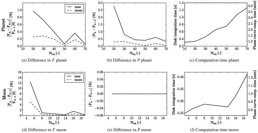
Figure 17: Analysis for the number of pixels along the equator $N_{\rm eq}$ of the planet (top) and moon (bottom). Shown are the maximum (solid line) and mean (dashed line) differences between results computed across the whole phase angle range and for consecutive values of $N_{\rm eq}$ values, for the reflected flux $F(\alpha)$ relative to $F(\alpha=0^{\circ})$ (a and d), and degree of polarization $P$ (b and e, note that for the moon $P=0$). Also shown is the computational time (in minutes) for the computation of a full phase curve (with 24 hour temporal resolution) and the average disk integration (c and f). For $N_{\rm eq}^{\rm p}$ (top), we used values of 10, 20, 30, 40, 50, 60, and 70, and for $N_{\rm eq}^{\rm m}$ (bottom), 3, 5, 8, 11, 14, 16, and 19.

References

- Agnor & Hamilton (2006) Agnor, C. B. & Hamilton, D. P. 2006, Nature, 441, 192
- Bailey (2007) Bailey, J. 2007, Astrobiology, 7, 320
- Barnes & Fortney (2003) Barnes, J. W. & Fortney, J. J. 2003, The Astrophysical Journal, 588, 545
- Benn (2001) Benn, C. R. 2001, The Moon and the Origin of Life (Dordrecht: Springer Netherlands), 61–66
- Beuzit et al. (2006) Beuzit, J.-L., Feldt, M., Dohlen, K., et al. 2006, The Messenger, 125
- Bott et al. (2016) Bott, K., Bailey, J., Kedziora-Chudczer, L., et al. 2016, Monthly Notices of the Royal Astronomical Society: Letters, 459, L109
- Buenzli & Schmid (2009) Buenzli, E. & Schmid, H. M. 2009, Astronomy & Astrophysics, 504, 259
- Cabrera & Schneider (2007) Cabrera, J. & Schneider, J. 2007, Astronomy & Astrophysics, 464, 1133
- Campbell et al. (1988) Campbell, B., Walker, G. A., & Yang, S. 1988, The Astrophysical Journal, 331, 902
- Canup & Ward (2006) Canup, R. M. & Ward, W. R. 2006, Nature, 441, 834
- Carciofi & Magalhães (2005) Carciofi, A. C. & Magalhães, A. M. 2005, ApJ, 635, 570
- de Haan et al. (1987) de Haan, J. F., Bosma, P. B., & Hovenier, J. W. 1987, AAP, 183, 371
- De Kok et al. (2011) De Kok, R., Stam, D., & Karalidi, T. 2011, The Astrophysical Journal, 741, 59
- de Kok & Stam (2012) de Kok, R. J. & Stam, D. M. 2012, Icarus, 221, 517
- De Pater & Lissauer (2015) De Pater, I. & Lissauer, J. J. 2015, Planetary sciences (Cambridge University Press), 22–55
- Domingos et al. (2006) Domingos, R. C., Winter, O. C., & Yokoyama, T. 2006, Monthly Notices of the Royal Astronomical Society, 373, 1227
- Forgan & Yotov (2014) Forgan, D. & Yotov, V. 2014, Monthly Notices of the Royal Astronomical Society, 441, 3513
- Ginski et al. (2018) Ginski, C., Benisty, M., van Holstein, R. G., et al. 2018, ArXiv e-prints 1805.02261
- Gratton et al. (2010) Gratton, R., Kasper, M., Vérinaud, C., Bonavita, M., & Schmid, H. M. 2010, Proceedings of the International Astronomical Union, 6, 343–348
- Han et al. (2014) Han, E., Wang, S. X., Wright, J. T., et al. 2014, Publications of the Astronomical Society of the Pacific, 126, 827
- Hansen & Travis (1974) Hansen, J. E. & Travis, L. D. 1974, Space Science Reviews, 16, 527
- Heller (2012) Heller, R. 2012, Astronomy & Astrophysics, 545, L8
- Heller (2014) Heller, R. 2014, The Astrophysical Journal, 787, 14
- Heller (2017) Heller, R. 2017, arXiv preprint arXiv:1701.04706
- Heller & Barnes (2013) Heller, R. & Barnes, R. 2013, Astrobiology, 13, 18
- Heller & Barnes (2015) Heller, R. & Barnes, R. 2015, International Journal of Astrobiology, 14, 335
- Heller et al. (2016) Heller, R., Hippke, M., & Jackson, B. 2016, The Astrophysical Journal, 820, 88
- Heller et al. (2014) Heller, R., Williams, D., Kipping, D., et al. 2014, Astrobiology, 14, 798
- Hippke (2015) Hippke, M. 2015, The Astrophysical Journal, 806, 51
- Hough & Lucas (2003) Hough, J. H. & Lucas, P. W. 2003, in ESA Special Publication, Vol. 539, Earths: DARWIN/TPF and the Search for Extrasolar Terrestrial Planets, ed. M. Fridlund, T. Henning, & H. Lacoste, 11–17
- Hough et al. (2003) Hough, J. H., Lucas, P. W., Bailey, J. A., & Tamura, M. 2003, in , 517–523
- Hovenier et al. (2004) Hovenier, J. W., van der Mee, C. V., & Domke, H. 2004, Transfer of polarized light in planetary atmospheres: basic concepts and practical methods, Vol. 318 (Springer Science & Business Media)
- Hovenier & van der Mee (1983) Hovenier, J. W. & van der Mee, C. V. M. 1983, AAP, 128, 1
- Karalidi et al. (2012) Karalidi, Stam, D. M., & Hovenier, J. W. 2012, A&A, 548, A90
- Kawata (1978) Kawata, Y. 1978, Icarus, 33, 217
- Keller et al. (2010) Keller, C. U., Schmid, H. M., Venema, L. B., et al. 2010, in , 77356G–77356G–13
- Kemp et al. (1987) Kemp, J. C., Henson, G. D., Steiner, C. T., & Powell, E. R. 1987, Nature, 326, 270
- Kipping (2009) Kipping, D. M. 2009, Monthly Notices of the Royal Astronomical Society, 392, 181
- Kipping (2010) Kipping, D. M. 2010, Monthly Notices of the Royal Astronomical Society: Letters, 409, L119
- Kipping (2011) Kipping, D. M. 2011, The Transits of Extrasolar Planets with Moons, 1st edn., Springer Theses (Springer Berlin Heidelberg), 127–164
- Kipping et al. (2009) Kipping, D. M., Fossey, S. J., Campanella, G., Schneider, J., & Tinetti, G. 2009, ArXiv e-prints 0911.5170
- Kipping et al. (2015) Kipping, D. M., Schmitt, A. R., Huang, X., et al. 2015, The Astrophysical Journal, 813, 14
- Kostogryz et al. (2015) Kostogryz, N., Yakobchuk, T., & Berdyugina, S. 2015, The Astrophysical Journal, 806, 97
- Kostogryz et al. (2011) Kostogryz, N., Yakobchuk, T., Morozhenko, O., & Vid’Machenko, A. 2011, Monthly Notices of the Royal Astronomical Society, 415, 695
- Lehmer et al. (2017) Lehmer, O. R., Catling, D. C., & Zahnle, K. J. 2017, The Astrophysical Journal, 839, 32
- Link (1969) Link, F. 1969, Eclipse Phenomena in Astronomy (Springer Berlin Heidelberg)
- Macintosh et al. (2014) Macintosh, B., Gemini Planet Imager instrument Team, Planet Imager Exoplanet Survey, G., & Observatory, G. 2014, in American Astronomical Society Meeting Abstracts, Vol. 223, American Astronomical Society Meeting Abstracts #223, 229.02
- Macintosh et al. (2015) Macintosh, B., Graham, J. R., Barman, T., et al. 2015, Science
- Marley & Sengupta (2011) Marley, M. S. & Sengupta, S. 2011, MNRAS, 417, 2874
- McClatchey et al. (1972) McClatchey, R., Fenn, R., Selby, J., Volz, F., & Garing, J. 1972, Optical Properties of the Atmosphere, AFCRL-72.0497 (U.S. Air Force Cambridge Research Labs)
- Morbidelli et al. (2012) Morbidelli, A., Tsiganis, K., Batygin, K., Crida, A., & Gomes, R. 2012, Icarus, 219, 737
- Murray & Correia (2010) Murray, C. D. & Correia, A. C. M. 2010, Keplerian Orbits and Dynamics of Exoplanets, ed. S. Seager, 15–23
- Reynolds et al. (1987) Reynolds, R. T., McKay, C. P., & Kasting, J. F. 1987, Advances in Space Research, 7, 125
- Rosenblatt et al. (2016) Rosenblatt, P., Charnoz, S., Dunseath, K. M., et al. 2016, Nature Geoscience
- Rossi et al. (2018) Rossi, L., Berzosa-Molina, J., & Stam, D. M. 2018, ArXiv e-prints 1804.08357
- Rossi & Stam (2017) Rossi, L. & Stam, D. 2017, Astronomy & Astrophysics
- Rossi & Stam (2018) Rossi, L. & Stam, D. M. 2018, Accepted for publication in A&A arXiv 1805.08686
- Rufu et al. (2017) Rufu, R., Aharonson, O., & Perets, H. B. 2017, Nature Geoscience
- Saar & Seager (2003) Saar, S. & Seager, S. 2003, ASP Conf. Ser., 294, 529
- Sartoretti & Schneider (1999) Sartoretti, P. & Schneider, J. 1999, Astronomy and Astrophysics Supplement Series, 134, 553
- Scharf (2006) Scharf, C. A. 2006, The Astrophysical Journal, 648, 1196
- Schneider et al. (2015) Schneider, J., Lainey, V., & Cabrera, J. 2015, International Journal of Astrobiology, 14, 191
- Seager et al. (2000) Seager, S., Whitney, B. A., & Sasselov, D. D. 2000, The Astrophysical Journal, 540, 504
- Sengupta (2016) Sengupta, S. 2016, The Astronomical Journal, 152, 98
- Sengupta & Marley (2016) Sengupta, S. & Marley, M. S. 2016, The Astrophysical Journal, 824, 76
- Simon et al. (2015) Simon, A., Szabó, G. M., Kiss, L., Fortier, A., & Benz, W. 2015, Publications of the Astronomical Society of the Pacific, 127, 1084
- Simon et al. (2007) Simon, A., Szatmáry, K., & Szabó, G. M. 2007, Astronomy & Astrophysics, 470, 727
- Snik & Keller (2013) Snik, F. & Keller, C. U. 2013, Astronomical Polarimetry: Polarized Views of Stars and Planets, ed. T. D. Oswalt & H. E. Bond (Dordrecht: Springer Netherlands), 175–221
- Stam et al. (2006) Stam, D., De Rooij, W., Cornet, G., & Hovenier, J. 2006, Astronomy & Astrophysics, 452, 669
- Stam (2003) Stam, D. M. 2003, in ESA Special Publication, Vol. 539, Earths: DARWIN/TPF and the Search for Extrasolar Terrestrial Planets, ed. M. Fridlund, T. Henning, & H. Lacoste, 615–619
- Stam (2008) Stam, D. M. 2008, A&A, 482, 989
- Stam et al. (2006) Stam, D. M., de Rooij, W. A., Cornet, G., & Hovenier, J. W. 2006, A&A, 452, 669
- Stam & Hovenier (2005) Stam, D. M. & Hovenier, J. W. 2005, A&A, 444, 275
- Stam et al. (2004) Stam, D. M., Hovenier, J. W., & Waters, L. B. F. M. 2004, A&A, 428, 663
- Stolker et al. (2017) Stolker, T., Min, M., Stam, D. M., et al. 2017, A&A, 607, A42
- Szabó et al. (2006) Szabó, G. M., Szatmáry, K., Divéki, Z., & Simon, A. 2006, Astronomy & Astrophysics, 450, 395
- Tinetti et al. (2016) Tinetti, G., Drossart, P., Eccleston, P., et al. 2016, in Proc. SPIE, Vol. 9904, Space Telescopes and Instrumentation 2016: Optical, Infrared, and Millimeter Wave, 99041X
- Wagner et al. (2016) Wagner, K., Apai, D., Kasper, M., et al. 2016, Science, 353, 673
- Wakker (2015) Wakker, K. F. 2015, Fundamentals of astrodynamics, Institutional Repository (TU Delft Library)
- Wiktorowicz & Laughlin (2014) Wiktorowicz, S. J. & Laughlin, G. P. 2014, The Astrophysical Journal, 795, 12
- Williams (2017) Williams. 2017, NASA Planetary Fact Sheet - Metric, retrieved on 10/01/2017 from https://nssdc.gsfc.nasa.gov/planetary/factsheet/
- Williams & Knacke (2004) Williams, D. & Knacke, R. 2004, Astrobiology, 4, 400
- Wolszczan & Frail (1992) Wolszczan, A. & Frail, D. A. 1992, Nature, 355, 145