Examples of renormalization group transformations for image sets

Abstract

Using the example of configurations generated with the worm algorithm for the two-dimensional Ising model, we propose renormalization group (RG) transformations, inspired by the tensor RG, that can be applied to sets of images. We relate criticality to the logarithmic divergence of the largest principal component. We discuss the changes in link occupation under the RG transformation, suggest ways to obtain data collapse, and compare with the two state tensor RG approximation near the fixed point.

I Introduction

Machine learning is a general framework for recognizing patterns in data without detailed human elaboration of the rules for doing so. As an example, a very general function, with many parameters (for example, thousands or millions) can be optimized on a training set, where the desired output is known. The problem is typically nonconvex and plagued by over-fitting problems, and so advanced methods are necessary in order to get reliable answers. One tool that has been exploited is principal component analysis (PCA), which reduces the dimensionality of the data to the most important “directions.” Immediately the practitioner of renormalization group (RG) methods recognizes an analogy, since the RG techniques are also supposed to identify the most important directions in an enlarged space of Hamiltonians. One of the motivations of the present research is to make this analogy more concrete.

A number of papers Li and Wang ; Bény ; Mehta and Schwab attempt to draw a connection between deep learning and the renormalization group as it appears in physics. However, the analogies between renormalization group flow and depth in a neural network would be strengthened if one could determine conditions under which fixed points can be identified. It would be helpful to show more explicitly how passing from one level to another in a neural network genuinely translates to a renormalization group transformation. There have been steps in the direction of making a full connection. For instance in Bény , the principle of causal influence is emphasized. That is, when descending in depth, only neighboring nodes should influence the outcome of a lower level node. We have also implemented this in a simple training scheme in earlier work Foreman et al. (2018). It can be called “cheap learning” because far fewer variational parameters are involved, due to the constraints of locality. In Mehta and Schwab it is emphasized that deep neural networks outperform shallower networks for reasons which may ultimately be understood in terms of the power of the renormalization group. Other topics related to machine learning, such as principal component analysis Bradde and Bialek have been previously interpreted in terms of the renormalization group (in this case momentum shells). Machine learning has also been used to identify phase transitions in numerical simulations Carrasquilla and Melko (2017); Wang (2016); Hu et al. (2017); Wetzel (2017).

RG transformations are usually defined in a space of couplings/Hamiltonians, but typically, it is not possible to write down Hamiltonians directly associated with images sets. In this article we propose RG transformations that can be applied to a specific set of images but which could be generalized for other image sets, and can also be understood analytically without any graphical representation. We use the well-studied example of the two-dimensional Ising model on a square lattice. The spin configurations generated with importance sampling provide images with black and white pixels. They have features that can be used to attempt to recognize the temperature used to generate them. However, constructing blocked Hamiltonians in configuration space is a difficult task which involves approximations that are difficult to improve. In other words, it is very difficult to explicitly construct the exact RG transformation mapping the original couplings among the Ising spins into coarse grained ones.

A better control on the RG transformation can be achieved by using the tensor renormalization group (TRG) method Levin and Nave (2007); Gu et al. (2009); Xie et al. (2012); Meurice (2013); Liu et al. (2013); Denbleyker et al. (2014); Yu et al. (2014). The starting point for this reformulation is the character expansion of the Boltzmann weights which is also used in the duality transformation Savit (1980). This leads to an exact expression of the partition function as a sum over closed paths which can be generated with importance sampling using the worm algorithm Prokof’ev and Svistunov (2001) and then pixelated. These samples will be our sets of images indexed by the temperature used to generate them. The procedure is reviewed in Sec. II.

The goal of a RG analysis is to study systems with large correlation lengths in lattice spacing units and iteratively replace them by coarser ones with a larger effective lattice spacing. This process is useful if we can tune a parameter such as the temperature towards its critical value. Typical image sets such as the MNIST data can be thought as “far from criticality” and the use of RG methods for such a data set may be of limited interest Foreman et al. (2018). Criticality may sometimes refer to the choice of parameters used in data analysis Enßlin and Frommert (2011). It seems crucial to introduce a systematic way to deal with the concept of criticality in ML.

The PCA is a standard method to analyze sets of images. In configuration space, the PCA analysis is identical to the study of the spin-spin correlation matrix. In particular, the largest eigenvalue $\lambda_{max}\$is directly connected to the magnetic susceptibility which diverges at criticality Wang (2016). In the loop representation (worms), we will show that $\lambda_{max}\$diverges logarithmically at criticality with a constant of proportionality which can be estimated quite precisely ($3/\pi$). This is explained in Sec. III. More generally, it seems reasonable to identify the criticality with the divergence of $\lambda_{max}\$.

The advantage of rewriting the high-temperature expansion in terms of tensors is that it allows a very simple blocking (coarse-graining) procedure where a group of sites is replaced by a single site. In the TRG approach the blocking procedure is local. This leads to simple and exact coarse-graining formulas because we can separate the links into two categories: one half of the links are inside the blocks and integrated over while the other half are kept fixed and ensure the communication among the blocks Meurice (2013). The main goal of this article is to relate blocking procedures that can be applied to sets of pixelated images, to approximate TRG transformations. A short summary of the TRG procedure is given in Sec. IV.

Having defined criticality, the next step is to define a RG transformation for sets of “legal” loop configurations, also called “worm configurations” later, sampled at various temperatures. In Sec. V, we propose a family of transformations which replaces two parallel links in a block by a single link carrying a specific value $x$. We call this procedure $1+1\rightarrow x$ hereafter. In the case $1+1\rightarrow 0$, the blocked images follow the same rules (for legal configurations) as the original ones. There is a clear analogy with the 2-state approximation for the TRG method which is described in the rest of the paper. In the 2-state TRG approximation, the average fraction of occupied links show a characteristic crossing at a critical point and a collapse when the distance to the critical point is appropriately rescaled at each iteration. The average fraction of occupied links in the blocked worm configurations (with $1+1\rightarrow 0$) show a somewhat similar behavior in the low temperature phase. However, on the high-temperature side, we observe a “merging” rather than a crossing. In Sec. VI, we provide explanations for the similarities and differences between the two procedures.

In Sec. VII we discuss an approximate 2-state TRG method to calculate the average number of bonds through several iterations.

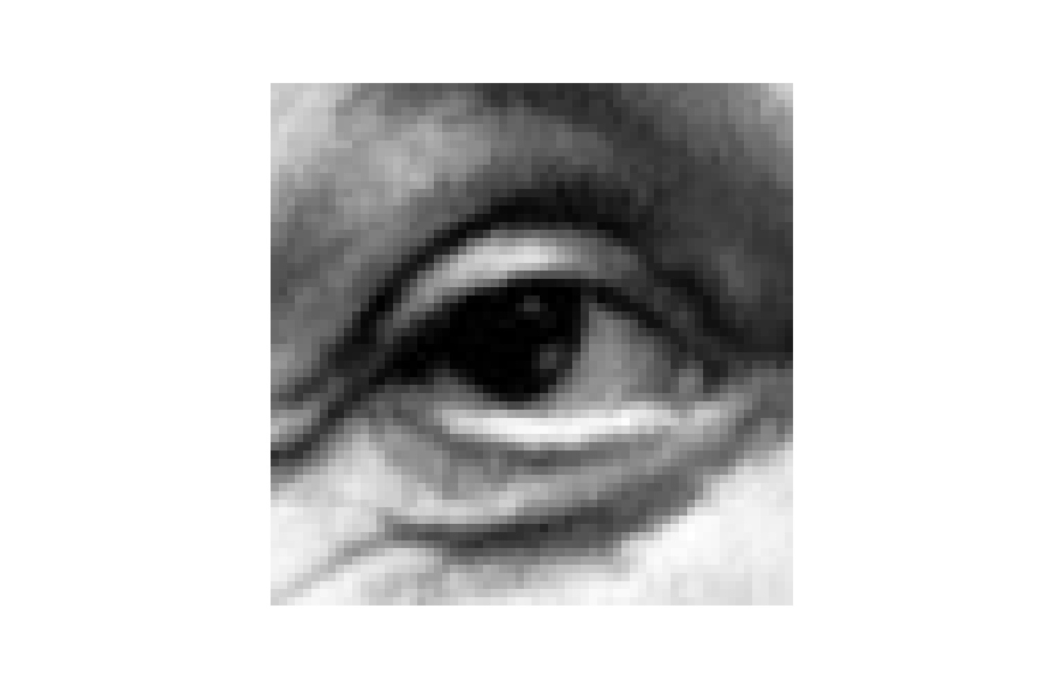
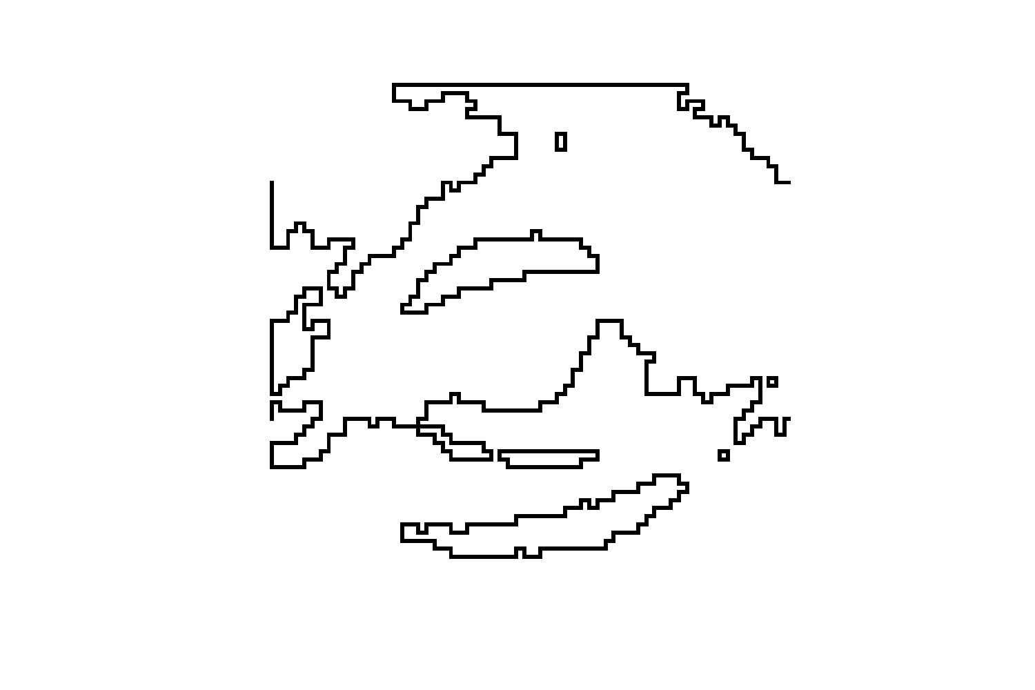
Figure 1: Picture of an eye with 4096 pixels; black and white version with a graycut at 0.72; boundaries of the black domains.

The worm configurations can be directly connected to spin configurations using duality Savit (1980): they are the boundary of the positive spin islands. This suggests that the methods discussed here could be applied to generic images. Boundaries of generic grayscale pictures can be defined by converting the picture to black and white pixels. A grayscale picture with gray values between 0 and 1 can be converted into an Ising spin configuration, by introducing a “graycut” below which the value is converted to 0 (spin down) and above which the value is converted to 1 (spin up). It is then possible to construct the boundaries of the spin up domains. This is illustrated in Fig. 1. Possible applications are discussed in Appendix B.

II From loops to images

In the following we consider the two-dimensional Ising model with spins $\sigma_{i}=\pm 1$ on a square lattice. The partition function reads

$$Z=\sum_{\{\sigma_{i}\}}e^{\beta\sum_{\langle i,j\rangle}\sigma_{i}\sigma_{j}},$$ (1)

where $\langle i,j\rangle$ denotes nearest neighbor sites on the square lattice. In some occasions we will use the notation $T=1/\beta$ for the temperature. The partition function can be rewritten by using the character expansion Prokof’ev (2004)

$$\exp(\beta\sigma)=\cosh(\beta)+\sigma\sinh(\beta),$$ (2)

and integrating over the spins. Factoring out the $\cosh(\beta)$, each link can carry a weight 1 when unoccupied or $t\equiv\tanh(\beta)$ when occupied. The integration over the spins guarantees that an even number of occupied links is coming out of each site Savit (1980). The set of occupied links then form a “legal graph” with $N_{b}$ occupied links. The partition function can then be written as sum over such legal graphs. If $\mathcal{N}(N_{b})$ denotes the number of legal graphs with $N_{b}$ links we can write:

$$Z=2^{V}(\cosh(\beta))^{2V}\sum_{N_{b}}t^{N_{b}}\mathcal{N}(N_{b})$$ (3)

Using the fact that $\tanh(\beta)=\exp(-2\tilde{\beta})$, with $\tilde{\beta}$ the inverse dual temperature, Eq. (3) has the same form as a spectral decomposition using a density of states and a Boltzmann weight (with $2N_{b}$ playing the role of the energy). Details of this reformulation can be found in Appendix A.1.

As shown in Appendix A.2, we can use derivatives of the logarithm of the partition function to relate $\langle N_{b}\rangle$ to the average energy, and the bond number fluctuations,

$$\langle\Delta_{N_{b}}^{2}\rangle\equiv\langle\left(N_{b}-\langle N_{b}\rangle\right)^{2}\rangle,$$ (4)

to the specific heat per site. From the logarithmic singularity of the specific heat we find that

$$\langle\Delta_{N_{b}}^{2}\rangle/V=-\frac{2}{\pi}\ln(|T-T_{c}|)+{\rm regular}.$$ (5)

In the following we use interchangeably the “bond” terminology, for instance in $N_{b}$ as in Prokof’ev (2004), and the link terminology more common in the lattice gauge theory context. In all our numerical simulations we use periodic boundary conditions which guarantees translation invariance.

We will show in Sec. IV that the new form of the partition function in Eq. (3) can also be written in an equivalent way as a sum of products of tensors with four indices contracted along the links of the lattice.

The contributions to Eq. (3) can be sampled using a worm algorithm Prokof’ev and Svistunov (2001) outlined in Appendix A.3. Using this algorithm, we generated multiple configurations at each temperature ($N_{configs}\approx 10,000$) which are then used for averaging. For example, we can calculate the average number of occupied bonds at a particular temperature by averaging over all configurations.

Using a legal graph (worm configuration), we can construct an image by introducing a lattice of $2L\times 2L$ pixels with a size of one half lattice spacing. One quarter of these pixels are attached to the sites, one quarter to the horizontal links and one quarter to the vertical links. The remaining quarter are in the middle of the plaquettes and always white. In this representation, each site, link, and plaquette are designated an individual pixel, where occupied links and their respective endpoints are colored black. An example of this representation is shown in Fig. 2.

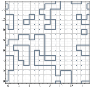
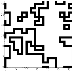
Figure 2: Legal worm configuration on an $L\times L$ lattice with periodic boundary conditions (top) and its equivalent representation as a $2L\times 2L$ black or white pixels (bottom).

We can then flatten each of these images into a vector $\mathbf{v}\in\mathbb{R}^{4V}$, with $v_{i}\in\{0,1\}$. This allows us to write the number of occupied bonds, in a single configuration, $N_{b}$ as

$$\sum_{j=bonds}v_{j}=N_{b}$$ (6)

III PCA and criticality

Having now sets of images for a range of temperatures, we can apply PCA Bishop (2006). PCA isolates the “most relevant” directions in the dataset. PCA is simply the computation of the eigenvalues $\lambda_{\alpha}$ and eigenvectors $u_{\alpha}$ of the covariance matrix for a dataset with $N$ configurations corresponding to a given temperature $\{{\bf v}^{n}\}_{n=1}^{N}$:

$$S_{ij}=\frac{1}{N}\sum_{n=1}^{N}(v_{i}^{n}-{\bar{v}}_{i})(v_{j}^{n}-{\bar{v}}_{j}).$$ (7)

In this equation, each sample ${\bf v}_{j}$ is a vector in $\mathbb{R}^{4V}$, labeled by the indices $i,j=1,\ldots,4V$. The PCA extracts solutions to

$$Su_{\alpha}=\lambda_{\alpha}u_{\alpha}$$ (8)

and orders them, in descending magnitude of $\lambda_{\alpha}$, which are all non-negative. The usefulness of PCA is that one can approximate the data (see for instance the discussion in Bishop (2006)) by the first $M$ principal components.

Illustrations of the PCA for the MNIST data can be found in Sec. 4 of Ref. Foreman et al. (2018), where we show the eigenvectors corresponding to the largest eigenvalues and the approximation of the data by subspaces of the largest eigenvalues of dimensions 10, 20 etc.

It should be noticed that the PCA is an analysis that can be performed for each temperature separately and not obviously connected to the closeness to criticality. However, we were able to find a relation between the largest PCA eigenvalue denoted $\lambda_{max}$ and the logarithmic divergence of the specific heat, namely

$$\lambda_{max}\simeq\frac{3}{2}\left\langle\Delta_{N_{b}}^{2}\right\rangle/V\simeq-\frac{3}{\pi}\ln(|T-T_{c}|).$$ (9)

This property was found by an approximate reasoning shown in Appendix A.2 and relies on two assumptions. The first one is that the eigenvector associated with $\lambda_{max}$ is proportional to $\langle\mathbf{v}\rangle$ which is invariant under translation by two pixels in either direction. The second assumption is that in good approximation we can neglect the contributions from sites that are visited twice (four occupied links coming out of one site). Numerically, only 4% of sites are visited twice near the critical temperature which justifies the second assumption. Fig. 3 provides an independent confirmation of the approximate validity of Eq. (9).

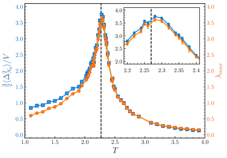
Figure 3: $\lambda_{max}$ and $\frac{3}{2}\left\langle\Delta_{N_{b}}^{2}\right\rangle/V$ vs. $T$, illustrating the relation between the eigenvalue corresponding to the first principal component and the logarithmic divergence of the specific heat. The inset shows a qualitative agreement near the critical temperature.

IV TRG coarse-graining

So far we have sampled the legal graphs of the high temperature expansion of the Ising model using the worm algorithm. An alternative approach is to use a tractable real-space renormalization group method known as the TRG Xie et al. (2012); Meurice (2013); Liu et al. (2013); Denbleyker et al. (2014); Yu et al. (2014).

In order to understand what we want to accomplish by blocking the loop  configuration, it is useful to first understand the evolution of a tensor element using the TRG method.

The tensor formulation used here connects easily with the worm formulation used in this paper. After the character expansion has been carried out, one is left with new integer variables on the links of the lattice with constraints on the sites which guarantee the sum of the link variables associated with that site is even. Therefore we build a tensor using this constraint and the surrounding link weights. The tensor has the form

$$T^{(i)}_{xx^{\prime}yy^{\prime}}(\beta)= \left[\tanh(\beta)\right]^{(n_{x}+n_{x^{\prime}}+n_{y}+n_{y^{\prime}})/2}$$ (10)

$$\times\delta_{n_{x}+n_{x^{\prime}}+n_{y}+n_{y^{\prime}},0\text{ mod }2}.$$ (11)

Here the notation being used is that this tensor is located at the $i$^th site of the lattice, $n_{\hat{\mu}}$ is the integer variable, taking value 0 or 1, on an adjacent link, and the Kronecker delta, $\delta_{i,j}$ is understood to be satisfied if the sum is even. By contracting these tensors together in the pattern of the lattice one recreates the closed-loop paths generated by the high-temperature expansion and exactly matches those paths which are sampled by the worm algorithm.

Using these tensors one can write a partition function for the Ising model that is exactly equal to the original partition function,

$$Z=2^{V}(\cosh(\beta))^{2V}\operatorname{Tr}\prod_{i}T^{(i)}_{xx^{\prime}yy^{\prime}}$$ (12)

where $\operatorname{Tr}$ means contractions (sums over 0 and 1) over the links.

The most important aspect of this reformulation is that it can be coarse-grained efficiently. The process is illustrated in Fig. 4 where four fundamental tensors have been contracted to form a new “blocked” tensor. This new tensor has a squared number of degrees of freedom for each new effective index. The partition function can be written exactly as

$$Z=2^{V}(\cosh(\beta))^{2V}\operatorname{Tr}\prod_{2i}T^{\prime(2i)}_{XX^{\prime}YY^{\prime}}\ ,$$

where $2i$ denotes the sites of the coarser lattice with twice the lattice spacing of the original lattice.

Figure 4: Illustration of the tensor blocking discussed in the text.

In practice, this exact procedure cannot be repeated indefinitely and truncations are necessary. This can be accomplished by projecting the product states into a smaller number of states that optimizes the closeness to the exact answer. A two-state projection is discussed in Meurice (2013) and will be followed hereafter. Note that in this procedure, $T_{0000}$ is factored out and the final expression for the other blocked tensors are given in these units. For definiteness we consider $T_{1100}$ which in the microscopic formulation is the weight associated with an horizontal line in a loop  configuration. By looking at the fixed point equation Meurice (2013) , one can see that that there is a high temperature fixed point where all the tensor elements except for $T_{0000}$ are zero and and a low temperature fixed point where all the tensor elements are one. In between these two limits, there is a non-trivial fixed point illustrated by the crossing of iterated values of $T_{1100}$ in Fig. 5. Note that because of the two-state approximation, the critical temperature $T_{c}$ is slightly higher than the exact one Meurice (2013). To be completely specific, the exact $T_{c}$ for the original model is $2/\ln(1+\sqrt{2})=2.269..$ while for the two state projection with the second projection procedure of Ref.Meurice (2013), it is $1/0.3948678=2.53249...$

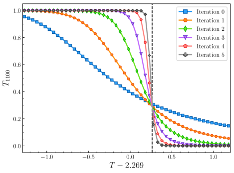
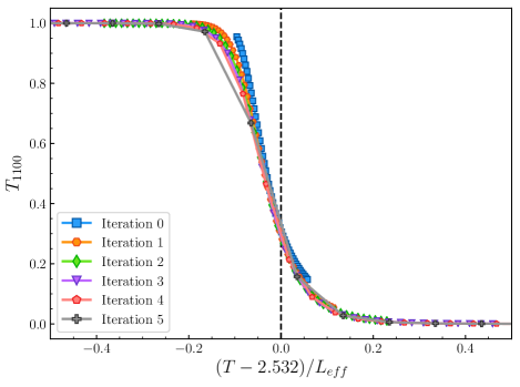
Figure 5: $T_{1100}$ vs $T-T_{c}$ for six successive iterations of the blocking transformation, beginning with an initial lattice $L=64$ (top); $T_{1100}$ vs. $(T-T_{c}^{(2s)})/L_{eff}$ illustrating the data collapse, where $T_{c}^{(2s)}$ is the critical temperature of the two state projection, beginning at iteration 0 on an $L=64$ lattice. (bottom).

It is easy to relate the properties of the iterated curves near the non-trivial fixed point using the linear RG approximation. Below we just state the results, for details and references see Meurice (2013). With the blocking procedure used, the scale factor is $b=2$. The eigenvalue in the relevant direction is $\lambda=b^{1/\nu}=2$ since $\nu=1$. In Fig. 5, on can see that near $T_{c}$, the height with respect to the crossing point nearly doubles each time, making the slope twice bigger each time. A nice data collapse can be reached by offsetting this effect by a rescaling by $\lambda$=2 the horizontal axis each iteration as shown in the bottom part of Fig. 5. In numerical calculations, we start with a finite $L$ (64 in Fig. 5) and then after $\ell$ iteration, we are left with an effective size $L_{eff}=L/b^{\ell}$.

The remainder of the paper will be dedicated towards obtaining data collapse for $\langle N_{b}\rangle$ calculated with successive blockings.

V Image coarse-graining

In an attempt to explicitly connect the ideas from RG theory to similar concepts in machine learning, we will implement a coarse-graining procedure directly on the images but in a way inspired by the TRG construction of Sec. IV. The construction relies on visual intuition and will be reanalyzed in the TRG context in Sec. VII.

As in the TRG coarse-graining procedure, the image is first divided up into blocks of $2\times 2$ squares, as shown in Fig. 6.

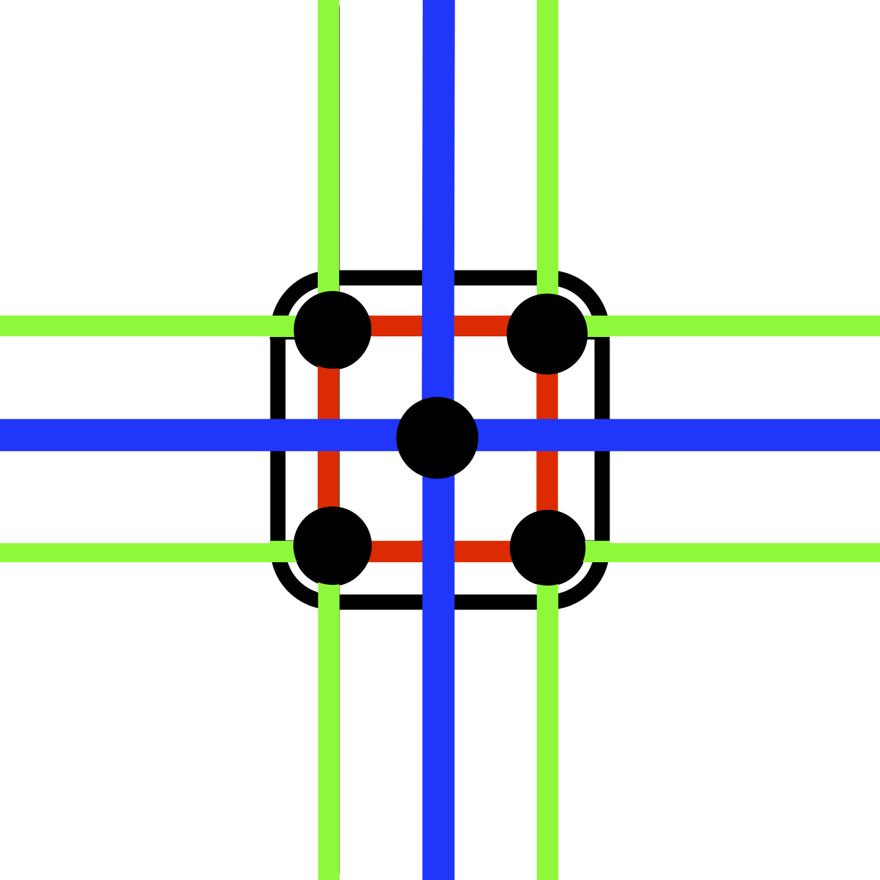
Figure 6: Illustration of an elementary block in the image consisting of four sites, four internal bonds (red), eight external bonds (green), and four blocked external bonds (blue).

Each of these $2\times 2$ squares are then replaced, or “blocked”, by a single site with bonds determined by the number of occupied external bonds in the original square. In doing so, we reduce the size of each linear dimension by a factor of two, resulting in a new blocked configuration whose volume is one-quarter the original. In particular, if a given block has exactly one external bond in a given direction, the blocked site retains this bond in the blocked configuration. This seems to be a natural choice. However, if a given block has exactly two external bonds in a given direction, we can consider several options. The simplest option is to neglect the double bond entirely, and we denote this blocking scheme by “$1+1\rightarrow 0$”. This approach respects the selection rule (conservation modulo 2) and has the advantage of maintaining the closed-path restriction. In other words with the $1+1\rightarrow 0$ option, the blocked image corresponds to a legal graph and the procedure can be iterated without introducing new parameters. This procedure is illustrated for a specific configuration on a $16\times 16$ lattice in Fig. 7.

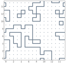
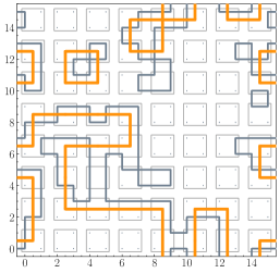
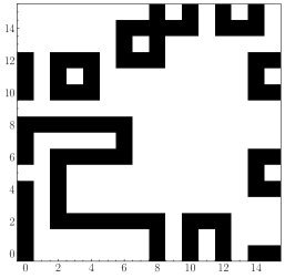
Figure 7: Illustration of the $1+1\rightarrow 0$ blocking procedure discussed in the text: original configuration (left); introduction of the blocks and replacement of single or double bounds according to the $1+1\rightarrow 0$ rule (middle); construction of the corresponding blocked image (right).

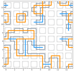
(a) $1+1=m$

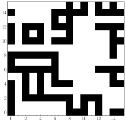
(b) $1+1\rightarrow 1$

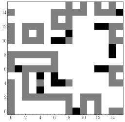
(c) $1+1\rightarrow 2$

Figure 16: Example of the different coarse-graining (“blocking”) procedures applied to a sample worm configuration generated at $T=2.0$. Note that in (16(a)) $m\in\{1,2\}$, and double bonds are represented by blue lines. (16(b)), (16(c)), illustrate the results of applying different weights to the so-called “double bonds” in the images representing a blocked configuration. Note that in (16(b)) $1+1\rightarrow 1$, double bonds are given the same weight as single bonds, and in (16(c)) $1+1\rightarrow 2$, double bonds are given twice the weight as single bonds, appearing twice as dark.

Alternatively, we can include this double bond in the blocked configuration, and give it some weight $m$ between 0 and 2. The examples of $m=$ 1 and 2 are denoted “$1+1\rightarrow 1$”, and “$1+1\rightarrow 2$” respectively and are shown in Fig. 16. This blocking procedure introduces new elements and iterations require more involved procedures. This is not discussed hereafter.

VI Partial data collapse for blocked images

In this section, we study the properties of $\langle N_{b}\rangle$ obtained for successive blockings with the $1+1\rightarrow 0$ rule starting with configurations on a $64\times 64$ lattice. A first observation is that the $1+1\rightarrow 0$ blocking preserves the location of the peak of the fluctuations $\langle\Delta_{N_{b}}^{2}\rangle$. In addition it is possible to stabilize this quantity for a few iterations by dividing by $L_{eff}\ln(L_{eff})$. This is illustrated in Fig. 8. However, a very different scaling appears for the last two iterations which may be due to the very short effective sizes (4 and 2). This indicates the last two iterations are very different from the previous ones.

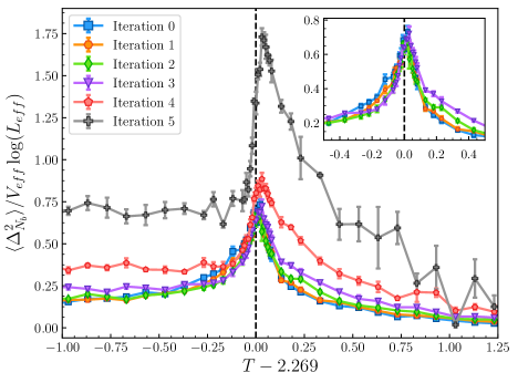
Figure 8: Fluctuations in the average number of bonds $\langle\Delta_{N_{b}}^{2}\rangle$ vs. temperature $T$ under iterated blocking steps beginning with an initial lattice size of $L=64$. The results are scaled by $1/V_{eff}\log(L_{eff})$ in order to demonstrate the data collapse near the critical temperature. This collapse is especially apparent in the inset, which shows the results under the first three blocking steps, with $L_{eff}=64,32,16$, and $8$.

We now consider $\langle N_{b}\rangle$ for successive iterations. The results are shown in Fig. 9. We see that in the low temperature side, the curves sharpen in a way similar to $T_{1100}$ in Fig. 5. However on the high temperature side, we observe a merging rather than a crossing. This can be explained as follows. In the high T regime occasionally a single loop, the size of a plaquette, forms. This is due to other configurations being highly suppressed. With the $1+1\rightarrow 0$ rule, one out of four possible plaquettes becomes a larger plaquette which exactly compensates the change in $V_{eff}$ which is also reduced by a factor of four. There are four kinds of plaquettes (see Fig. 7): those inside the blocks (they disappear after blocking), those between two neighboring blocks in the vertical or horizontal direction (these are double links between the blocks and so they disappear with the $1+1\rightarrow 0$ rule), and finally those which share a corner with four blocks (they generate a larger plaquette); this type can be seen at (4, 12) in Fig. 7.

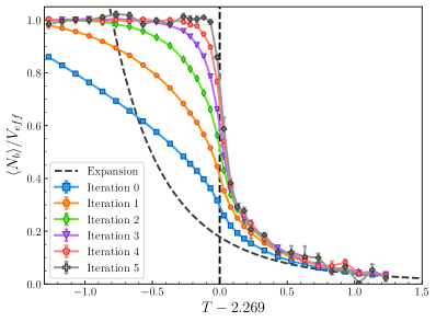
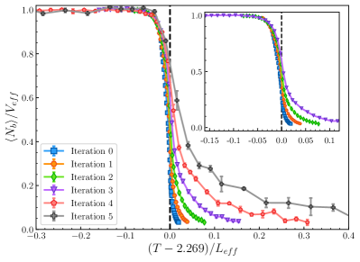
Figure 9: Average number of bonds $\langle N_{b}\rangle$ vs. temperature $T$ under iterated blocking steps beginning with an initial lattice size of $L=64$ (left). The dashed black line illustrates the high temperature expansion, showing that the dominant configurations are those consisting of small, isolated plaquettes. Average number of bonds $\langle N_{b}\rangle$ vs. the rescaled temperature $(T-2.269)/L_{eff}$ under successive blocking steps (right). Iteration 0 represents the original lattice before blocking, with $L_{eff}=64$.

We now attempt to obtain data collapse for $\langle N_{b}\rangle/V_{eff}$ by performing a rescaling of the temperature axis with respect to the critical value as in Fig. 5. After this rescaling by a factor 2 at each iteration, we observe a reasonable collapse on the low-temperature side. On the high temperature side, since the unrescaled curves merge, the rescaling splits them and there is no collapse on that side. This is illustrated in the bottom part of Fig. 9.

VII TRG calculation of $\langle N_{b}\rangle$

Using the tensor method we were able to calculate $\langle N_{b}\rangle$ to compare with the worm algorithm. Consider the equation for $\langle N_{b}\rangle$ with $N_{b}=\sum_{l}n_{l}$ the sum over bond numbers at every link.

$$\langle N_{b}\rangle=\frac{1}{Z}\sum_{\{n\}} \left(\sum_{l}n_{l}\right)\left(\prod_{l}\tanh^{n_{l}}(\beta)\right)$$ (13)

$$\times\left(\prod_{i}\delta^{(i)}_{n_{x}+n_{x^{\prime}}+n_{y}+n_{y^{\prime}},0\text{ mod }2}\right).$$

This expression can be seen as $\langle N_{b}\rangle=\sum_{l}\langle n_{l}\rangle$, and because of translation and $90^{\circ}$ rotational invariance, all $\langle n_{l}\rangle$ are equal. Thus, it is enough to calculate $\langle n_{l}\rangle$ for one particular link (just call it $\langle n\rangle$) and multiply it by $2V$: $\langle N_{b}\rangle=2V\langle n\rangle$.

To calculate $\langle n\rangle$, it amounts to associating an $n$ with one particular link on the lattice. This alters two tensors on the lattice such that the two tensors which contain that link as indices are now defined as

$$\tilde{T}^{(1)}_{n_{x}n_{x^{\prime}}n_{y}n_{y^{\prime}}} =\sqrt{n_{x}}T_{n_{x}n_{x^{\prime}}n_{y}n_{y^{\prime}}}(\beta)$$ (14)

$$\tilde{T}^{(2)}_{n_{x}n_{x^{\prime}}n_{y}n_{y^{\prime}}} =\sqrt{n_{x^{\prime}}}T_{n_{x}n_{x^{\prime}}n_{y}n_{y^{\prime}}}(\beta)$$ (15)

where $x$ and $x^{\prime}$ were chosen without loss of generality. It could just as well have been chosen as $y$ and $y^{\prime}$. One can see that when these two tensors are contracted along their shared link, the product picks up a factor of $n$ for that link, which when combined with the other tensors in the lattice, and divided by $Z$, yields $\langle n\rangle$.

Knowing the above, one is free to block and construct the partition function, $Z$, and $\langle n\rangle$. This can be done by blocking symmetrically in both directions, or by constructing a transfer matrix by contracting only along a time-slice. This is shown in Fig. 10. In practice contracting to build a transfer matrix is optimum since one direction of the lattice is never renormalized and allows the easy calculation of $\langle n\rangle$.

Figure 10: A pictorial representation of the transfer matrix made by contracting a fundamental tensor along a single time-slice.

What is described in the previous section is a method to calculate $\langle n\rangle$ for the original, fine, lattice. However, one can also calculate the same quantity for a coarse lattice. The actual blocking method is essentially identical, with a small exception. Instead of contracting the fundamental tensor to the desired lattice size, one contracts a blocked tensor to the desired lattice size.

For example, if one wanted to calculate $\langle N_{b}\rangle$ for a $32\times 32$ lattice, one could contract the fundamental tensor along a time slice with itself five times. This would give a $2^{32}\times 2^{32}$ transfer matrix which could be used to build the whole partition function. Now, under a single coarse-graining step the $32\times 32$ lattice becomes a $16\times 16$ lattice of blocks. Therefore, to build this, one could contract four fundamental tensors in a block and consider this a new, effective fundamental tensor. This is shown in Fig. 4. Then one repeats the same steps to construct the transfer matrix, however only contracting four times with itself to create a matrix representing 16 lattice sites of the blocked tensor.

To actually calculate $\langle n\rangle$ by building the transfer matrix, one can take the final tensor, prior to contracting the dangling spatial indices, and multiply by $\sqrt{n}$ against the indices $n_{x}$ and $n_{x^{\prime}}$. This is shown for the unblocked case in Fig. 11, however the procedure is identical for the blocked case once the blocked tensor has been constructed.

Figure 11: By multiplying the remaining free spatial indices by $\sqrt{n}$ and contracting for periodic boundary conditions in space we form an “impure” transfer matrix. Combining the resultant matrix with the original transfer matrix allows one to calculate $\langle n\rangle$.

This is also the point where one can choose the level of approximation one will use in the blocking. For instance one could choose that the state $|1\;1\rangle\rightarrow|0\rangle$ and assign $n=0$ to that state. Alternatively one could preserve $N_{b}$ and let $|1\;1\rangle\rightarrow|2\rangle$ and assign $n=2$ to that state. This procedure was found to agree with the results obtained by changing the pixels of the worm configurations.

Once the original transfer matrix has been constructed, as well as the matrix with the insertion of $n$ along a single link, one can combine these to find $\langle n\rangle$. This is done by simple matrix multiplication:

$$\langle n\rangle=\frac{1}{Z}\mathop{{\hbox{Tr}\,}}\nolimits[\underbrace{\mathbb{T}\cdots\mathbb{T}^{\prime}\cdots\mathbb{T}}_{N_{\tau}}]$$ (16)

with

$$Z=\mathop{{\hbox{Tr}\,}}\nolimits[\mathbb{T}^{N_{\tau}}].$$ (17)

Here $\mathbb{T}$ represents the transfer matrix built by contracting tensors along a time slice, and $\mathbb{T}^{\prime}$ represents the single (“impure”) transfer matrix at a time-slice with a single bond multiplied by $n$. Since the lattice has Euclidean temporal extent, $N_{\tau}$, there are that many matrices multiplied in each case. The values of $\langle N_{b}\rangle/V_{eff}$ obtained with this procedure are shown in Fig. 12. The rescaling by 2 at each iteration provides a good data collapse on both sides of the transition.

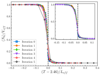
Figure 12: $\langle N_{b}\rangle$ vs $(T-2.46)$ under successive blocking steps calculated using 2-state HOTRG (left). $\langle N_{b}\rangle$ vs $(T-2.46)/L_{eff}$ under successive blocking steps calculated using 2-state HOTRG (right).

VIII Conclusions

In summary, we have motivated, constructed and applied a RG transformation to sets of worm configurations at various temperature. This transformation is approximate and the coarse-grained configurations are themselves worm configurations. This allows multiple iterations. We monitored the bond density at successive iterations and compared them with a two-state TRG approximation. We found clear similarities in the low-temperature side, where data collapse is observed for both procedures when the distance to the critical point is rescaled at each iteration. In the high-temperature phase, only the TRG approximation shows good data collapse.

Can the procedure developed here be applied to the boundary of arbitrary sets of images as illustrated in the introduction? The gray cutoff could be used as a tunable parameter. However, in the limiting cases of a zero (one) gray cutoff we have uniform black (white) images which are both similar to the high-temperature phase, and we do not expect a phase transition. Applications to the CIFAR dataset are discussed in Appendix B and confirm this point of view.

A better understanding of RG concepts in machine learning could enhance physics discovery, especially in the context of simulation and modeling of physical systems at a fundamental level Shanahan et al. (2018). The general idea is to render computational tools “smart,” i.e., that they would learn features and patterns without the intervention of a human “assistant,” and would, in the best possible scenario, guide the direction of further simulations. This could accelerate and deepen the process of understanding and characterizing the complex systems that are deemed important in pure and applied physics.

Appendix A Technical results

A.1 Loop representation

We can rewrite the Ising partition function in terms of bonds between neighboring sites $\langle i,j\rangle$. The allowed bond configurations are concisely described by concepts in graph theory, because they form edges (bonds) between neighboring vertices (sites). Making use of well-known identities allows for the partition function to be written in the following high-temperature expansion:

$$Z =2^{|V|}\cosh^{|E|}\beta\sum_{\Gamma\in{\cal C}(G)}\tanh^{|\Gamma|}\beta$$ (18)

$$=2^{|V|}\cosh^{|E|}\beta\sum_{|\Gamma|}\tanh^{|\Gamma|}\beta~{}n(|\Gamma|)$$ (19)

The notation is as follows. We have a graph $G=(V,E)$ that describes our lattice, where $V$ are the vertices and $E$ are the edges, which are the bonds between neighboring sites. If we restrict ourselves to subgraphs with only occupied bonds allowed by the Ising model, then the degree of each vertex is even. This is the number of bonds emanating from a particular vertex. The set of edges of such a subgraph is described as being “Eulerian.” The space of all such sets of edges is known as the cycle space ${\cal C}(G)$. The notation $|V|$, $|E|$, $|\Gamma|$ denotes the number of elements in each set (cardinality). In the second line, $n(|\Gamma|)$ counts the multiplicity of subgraphs of cardinality $|\Gamma|$, and is zero when $|\Gamma|$ does not correspond to a “legal” subgraph.

We now specialize the presentation to the the case of the two-dimensional Ising model on a square lattice with periodic boundary conditions. In this case $|V|$ is $V=L^{2}$, the volume that we express in lattice units, and $|E|=2V$. We introduce the notation $t\equiv\tanh(\beta)$ and we call $N_{b}$ the number of bonds in a graph (values taken by $|\Gamma|$). With these notations we recover Eq. 3.

It is this bond formulation that is the basis of both random cluster algorithms Swendsen and Wang (1987) and worm algorithms Prokof’ev and Svistunov (2001). In this paper we utilize the latter. Both of these classes of algorithms have the benefit of significantly avoiding critical slowing down. This is essential near the critical temperature $T_{c}$.

A.2 Heat capacity

One striking feature of the second order transition for the two-dimensional Ising model is the logarithmic divergence of the specific heat density at the critical temperature $T_{c}$. In this section, we review the way the specific heat can be calculated with the worm algorithm and we check our answer with the exact finite volume expressions Kaufman (1949).

Using the standard thermodynamical formula for the average energy

$$\langle E\rangle=-\frac{\partial}{\partial\beta}\ln Z,$$ (20)

with the expression (3) of $Z$, we get

$$\langle E\rangle=-\tanh(\beta)\left(2V+\frac{\langle N_{b}\rangle}{\sinh^{2}(\beta)}\right),$$ (21)

where we define

$$\langle f(N_{b})\rangle\equiv\sum_{N_{b}}f(N_{b})t^{N_{b}}n(N_{b})/\sum_{N_{b}}t^{N_{b}}n(N_{b})$$ (22)

We can then use

$$C_{V}=\frac{\partial\langle E\rangle}{\partial T},$$ (23)

to write

$$\frac{C_{V}}{V}=\beta^{2}\bigg{[} \frac{2}{\cosh^{2}(\beta)}-\frac{4\cosh(2\beta)}{\sinh(2\beta)}\frac{\langle N_{b}\rangle}{V}$$ (24)

$$+\left(\frac{2}{\sinh(2\beta)}\right)^{2}\frac{\langle(N_{b}-\langle N_{b}\rangle)^{2}\rangle}{V}\bigg{]}$$ (25)

Since $\frac{\langle N_{b}\rangle}{V}\leq 2$ (in two dimensions), the only possibly divergent part is the variance of $N_{b}$ per unit volume $\langle\Delta_{N_{b}}^{2}\rangle$ defined in Eq. (4). The singularity near $T_{c}$ is known from Onsager’s solution:

$$\frac{C_{V}}{V}=-\frac{2}{\pi}\left(\ln(1+\sqrt{2})\right)^{2}\ln\left(|T-T_{c}|\right)+\text{regular}.$$ (26)

This implies Eq. (5).

A.3 Monte Carlo implementation

We can proceed to sample the closed path configuration space using the worm algorithm Prokof’ev and Svistunov (2001). A single Monte Carlo step is outlined below.

1. Randomly select a starting point on the lattice $(i_{0},j_{0})$.

2. Propose a move to a neighboring site $(i^{\prime},j^{\prime})$, selected at random.

3. If no link is present between these two sites, a bond is created with acceptance probability $P=\min\{1,\tanh{\beta}\}$. If the bond is accepted, we update the bond number for the present worm, $n_{b}=n_{b}+1$.

4. If a link already exists between the two sites, it is removed with probability $P=1$.

5. If $(i^{\prime},j^{\prime})=(i_{0},j_{0})$, i.e. we have a closed path, go to (1.). Otherwise, $(i^{\prime},j^{\prime})\neq(i_{0},j_{0})$, go to (2.)

The number of necessary Monte Carlo steps required to achieve sufficient statistics varies with the lattice size, thermalization time, and temperature. After each step, we calculate the energy in terms of the average number of active bonds $N_{b}$, and consider the system to be thermalized when fluctuations between subsequent values of the energy are less than $1\times 10^{-3}$. We then save the resulting configuration, along with the final values for all physical quantities of interest. This process is then repeated many times over a range of different temperatures to generate sufficient statistics for physical observables. All errorbars are calculated using the block jackknife resampling technique.

A.4 Tests

The above formulas have been used to calculate $C_{V}$. Precise checks were performed by comparing with with the exact results obtained from Ref. Kaufman (1949). The agreement can be seen in Fig. 13. Results for other lattice sizes that we have simulated are similar.

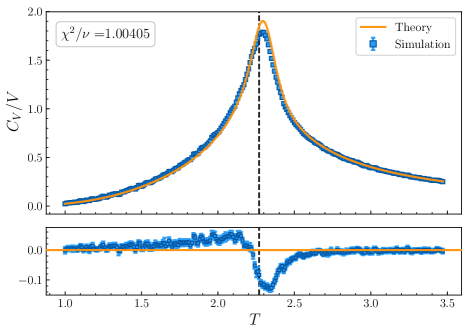
Figure 13: Comparison of the worm Monte Carlo computation of the specific heat $C_{v}$ versus temperature and the exact results using the formula in Kaufman (1949), for an $L=32$ lattice. It can be seen that the agreement is excellent, except for a slight deviation at the critical temperature, where Monte Carlo algorithms tend to face difficulties with critical slowing down. This is mostly addressed with the worm algorithm, in terms of having a dynamical scaling exponent that is zero rather than two, but there is (as can be seen), still a residual suppression of fluctuations in the immediate vicinity of $T_{c}$.

A.5 Conjecture about $\lambda_{max}$

Using the Monte Carlo algorithm outlined above, we can calculate the average number of occupied bonds at a particular temperature by averaging over all configurations

$$\langle N_{b}\rangle \equiv\frac{1}{N_{configs}}\sum_{n=1}^{N_{configs}}N_{b}^{(n)}$$ (27)

$$=\left\langle\sum_{j=bonds}v_{j}\right\rangle$$ (28)

$$=2V\langle\mathbf{v}_{b}\rangle\Longrightarrow$$ (29)

$$\langle\mathbf{v}_{b}\rangle =\frac{\langle N_{b}\rangle}{2V},$$ (30)

where we’ve defined $\langle\mathbf{v}_{b}\rangle$ to be the average occupation of bonds, $N_{b}^{(n)}$ to be the number of occupied bonds in the $n$-th configuration, and we’ve used (6) in the second line. If we consider graphs with no self-intersections,

$$\sum_{j=bonds}v_{j}=\sum_{j=sites}v_{j}.$$ (31)

For small $\beta$ (high $T$) this can be a good approximation,

$$\left\langle\sum_{j=bonds}v_{j}\right\rangle \simeq\left\langle\sum_{j=sites}v_{j}\right\rangle\Longrightarrow$$ (32)

$$\langle\mathbf{v}_{b}\rangle \simeq\frac{1}{2}\langle\mathbf{v}_{s}\rangle$$ (33)

This agrees with our intuition, that the average image $\langle\mathbf{v}\rangle$ should resemble a “tablecloth”, where the site pixels are twice as dark as the link pixels. This can be seen clearly in Fig. 14.

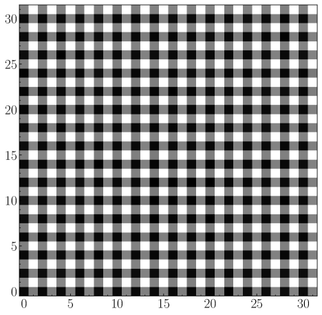
Figure 14: Average image $\langle\mathbf{v}\rangle$ calculated for the $L=16$ lattice at $T=2.0$, illustrating the tablecloth-like appearance.

For a general graph, a link is shared by two sites (its endpoints), whereas a site can be shared either by 0, 2, or 4 bonds. If the site is shared by two bonds, it is only visited once, denoted $sites^{(1)}$, and if it is shared by four bonds, it is visited twice, denoted $sites^{(2)}$. This allows us to break up the sum over bonds into two terms

$$\sum_{j=bonds}v_{j}=\frac{2}{2}\sum_{j=sites^{(1)}}v_{j}+\frac{4}{2}\sum_{j=sites^{(2)}}v_{j}$$ (34)

Rearranging and taking averages gives

$$\left\langle\sum_{j=sites^{(1)}}v_{j}\right.+ \left.\sum_{j=sites^{(2)}}v_{j}\right\rangle$$ (35)

$$=\left\langle\sum_{j=bonds}v_{j}-\sum_{j=sites^{(2)}}v_{j}\right\rangle$$ (36)

$$=\left\langle\sum_{j=sites}v_{j}\right\rangle$$ (37)

$$=V\left\langle\mathbf{v}_{s}\right\rangle$$ (38)

$$=\left\langle\sum_{j=bonds}v_{j}\right\rangle-\left\langle\sum_{j=sites^{(2)}}v_{j}\right\rangle$$ (39)

$$=2V\langle\mathbf{v}_{b}\rangle-\left\langle N_{sites^{(2)}}\right\rangle\Longrightarrow$$ (40)

$$\frac{\left\langle N_{sites^{(2)}}\right\rangle}{V} =2\langle\mathbf{v}_{b}\rangle-\langle\mathbf{v}_{s}\rangle.$$ (41)

We can rewrite the last equation using (30)

$$\langle\mathbf{v}_{s}\rangle=\frac{\langle N_{b}\rangle}{V}-\frac{\langle N_{sites^{(2)}}\rangle}{V}.$$ (42)

This suggests that a departure from a perfect tablecloth ($\langle\mathbf{v}_{s}\rangle=2\langle\mathbf{v}_{b}\rangle$) contains information. Another useful construct is the covariance matrix,

$$C_{ij} =\left\langle\left(v_{i}-\langle\mathbf{v}\rangle_{i}\right)\left(v_{j}-\langle\mathbf{v}\rangle_{j}\right)^{T}\right\rangle$$ (43)

$$=\frac{1}{N_{configs}}\sum_{n=1}^{N_{configs}}\left(v_{i}^{(n)}-\langle\mathbf{v}\rangle_{i}\right)\left(v_{j}^{(n)}-\langle\mathbf{v}\rangle_{j}\right)^{T},$$ (44)

where we’ve defined $v_{k}^{(n)}$ to be the grayscale value of the $k$-th pixel in the $n$-th sample configuration, and $\langle\mathbf{v}\rangle_{k}$ is the average grayscale value of the $k$-th pixel over the set of configurations.

At some fixed temperature, the covariance matrix, $C\in\mathbb{R}^{N_{configs}\times 4L^{2}}$, where $N_{configs}$ is the number of sample configurations (images), with each configuration flattened into a vector of length $4L^{2}$. We can then perform a singular value decomposition (SVD) on the covariance matrix,

$$C=W\Lambda W^{T}$$ (45)

where $W$ is a $4L^{2}\times 4L^{2}$ matrix whose columns ($\mathbf{w}_{k}$) are the eigenvectors of $C$, and $\Lambda$ is the diagonal matrix of the absolute value of the eigenvalues $\lambda^{(k)}$ of $C$, arranged in decreasing order. Without loss of generality, we can assume the eigenvectors $\mathbf{w}_{k}$ are real and normalized such that $\mathbf{w}_{k}^{T}\mathbf{w}_{k}=1$. Thus, we can write

$$C\mathbf{w}_{k} =\lambda^{(k)}\mathbf{w}_{k}$$ (46)

$$\mathbf{w}_{k}^{T}C\mathbf{w}_{k} =\lambda^{(k)}$$ (47)

For our purposes, we are interested in the first principal component, with eigenvalue $\lambda^{(1)}\equiv\lambda_{1}$ and corresponding eigenvector $\mathbf{w}_{1}$.

We conjectured that the first principal component, $\mathbf{w}_{1}$ of the covariance matrix $C$ is directly proportional to the average worm configuration (image) $\langle\mathbf{v}\rangle$, i.e.

$$\mathbf{w}_{1}\propto\langle\mathbf{v}\rangle$$ (48)

From our results in II, we can write

$$\langle\mathbf{v}\rangle^{2} =\langle\mathbf{v}\rangle^{T}\langle\mathbf{v}\rangle$$ (49)

$$=2V{\langle\mathbf{v}_{b}\rangle}^{2}+V{\langle\mathbf{v}_{s}\rangle}^{2}$$ (50)

This suggests that

$$\mathbf{w}_{1}=\frac{\langle\mathbf{v}\rangle}{\sqrt{(2{\langle\mathbf{v}_{b}\rangle}^{2}+{\langle\mathbf{v}_{s}\rangle}^{2})V}}$$ (51)

Moreover, we can write

$$\sum_{i}\bigg{(}v_{i}^{(n)} -\langle\mathbf{v}\rangle_{i}\bigg{)}\langle\mathbf{v}\rangle_{i}$$ (52)

$$=\bigg{\{}{\langle\mathbf{v}_{b}\rangle}\sum_{j=bonds}v_{j}^{(n)}+{\langle\mathbf{v}_{s}\rangle}\sum_{j=sites}v_{j}^{(n)}$$ (53)

$$\quad\quad\quad-\left(2V{\langle\mathbf{v}_{b}\rangle}^{2}+V{\langle\mathbf{v}_{s}\rangle}^{2}\right)\bigg{\}}$$ (54)

$$=\bigg{\{}{\langle\mathbf{v}_{b}\rangle}N_{b}^{(n)}+{\langle\mathbf{v}_{s}\rangle}N_{s}^{(n)}$$ (55)

$$\quad\quad\quad-V\left(2{\langle\mathbf{v}_{b}\rangle}^{2}+{\langle\mathbf{v}_{s}\rangle}^{2}\right)\bigg{\}}$$ (56)

$$=\bigg{\{}{\langle\mathbf{v}_{b}\rangle}\left(N_{b}^{(n)}-\langle N_{b}\rangle\right)$$ (57)

$$\quad\quad\quad+{\langle\mathbf{v}_{s}\rangle}\left(N_{s}^{(n)}-\langle N_{s}\rangle\right)\bigg{\}}$$ (58)

$$\equiv{\langle\mathbf{v}_{b}\rangle}\Delta_{N_{b}}^{(n)}+{\langle\mathbf{v}_{s}\rangle}\Delta_{N_{s}}^{(n)}$$ (59)

From this, we can extract a relationship between the eigenvalue corresponding to the first principal component, $\lambda^{(1)}$ and the fluctuations $\Delta_{N_{b}}$ and $\Delta_{N_{s}}$,

$$\mathbf{w}_{1}^{T}C\mathbf{w}_{1} =\lambda^{(1)}$$

$$=\frac{1}{N_{configs}}\sum_{n=1}^{N_{configs}}({\langle\mathbf{v}_{b}\rangle}^{2}\left(\Delta_{N_{b}}^{(n)}\right)^{2}$$

$$+2{\langle\mathbf{v}_{b}\rangle}{\langle\mathbf{v}_{s}\rangle}\Delta_{N_{b}}^{(n)}\Delta_{N_{s}}^{(n)}+{\langle\mathbf{v}_{s}\rangle}^{2}\left(\Delta_{N_{s}}^{(n)}\right)^{2})$$

$$\frac{1}{\left(2{\langle\mathbf{v}_{b}\rangle}^{2}+{\langle\mathbf{v}_{s}\rangle}^{2}\right)}$$

Now, if we consider the high temperature approximation where sites only have single visits (no self-intersections), ${\langle\mathbf{v}_{s}\rangle}\simeq 2{\langle\mathbf{v}_{b}\rangle}$, $\langle N_{s}\rangle\simeq\langle N_{b}\rangle$, and $\Delta_{N_{b}}\simeq\Delta_{N_{s}}$, we have that $2{\langle\mathbf{v}_{b}\rangle}^{2}+{\langle\mathbf{v}_{s}\rangle}^{2}\simeq 6{\langle\mathbf{v}_{b}\rangle}^{2}$. and

$$\lambda_{1} \simeq\frac{{\langle\mathbf{v}_{b}\rangle}^{2}}{N_{configs}}\frac{9}{6{\langle\mathbf{v}_{b}\rangle}^{2}}\sum_{n=1}^{N_{configs}}\left(\Delta_{N_{b}}^{(n)}\right)^{2}$$ (60)

$$=\frac{3}{2}\frac{1}{N_{configs}}\sum_{n=1}^{N_{configs}}\left(\Delta_{N_{b}}^{(n)}\right)^{2}$$ (61)

$$=\frac{3}{2}\left\langle\Delta_{N_{b}}^{2}\right\rangle.$$ (62)

A justification for making this approximation can be seen in Fig. 15.

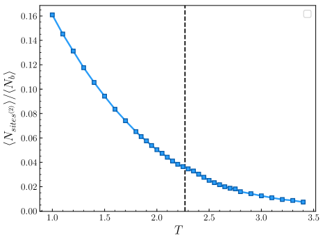
Figure 15: Ratio of the number of twice visited sites $\langle N_{sites^{2)}}\rangle$ to the average number of bonds $\langle N_{b}\rangle$ versus temperature, for the $L=32$ lattice. This clearly justifies our approximation ${\langle\mathbf{v}_{s}\rangle}\simeq 2{\langle\mathbf{v}_{b}\rangle}$, where we ignore the contribution from twice visited sites.

A.6 Illustration of alternate blockings

Appendix B Possible applications: From Images to Loops

Having better understood how these RG transformations can be used to describe the 2D Ising model near criticality, we began to look for possible applications to real-world datasets. For our analysis, we used the CIFAR-10 Krizhevsky and Hinton (2009) image set consisting of $60,000$ $32\times 32$ color images in 10 classes. First, each of the images were converted to a grayscale with pixel values in the range $[0,1]$. Next, a grayscale cutoff value was chosen so that all pixels with values below the cutoff would become black, and pixels above the cutoff would become white, resulting in images consisting entirely of black and white pixels. Finally, each of these images were converted to ‘worm-like’ images by drawing the boundaries separating black and white collections of pixels. An example of these preprocessing steps are illustrated in Fig. 17.

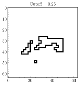
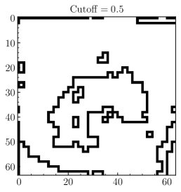
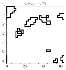
Figure 17: Example of preprocessing steps for converting CIFAR-10 images to ‘worm-like’ images.

This process was carried out on a mini-batch consisting of 500 randomly selected images from the CIFAR-10 image set. For each image in our mini-batch, we calculated $\langle N_{b}\rangle$ and $\langle\Delta_{N_{b}}^{2}\rangle$ over a range of grayscale cutoff values in $[0,1]$ in steps of $0.02$. Each of these images were then iteratively blocked using the $(1+1\rightarrow 0)$ blocking procedure described in Sec. IV, calculating $\langle N_{b}\rangle$ and $\langle\Delta_{N_{b}}^{2}\rangle$ for each successive blocking step, as shown in Fig. 18.

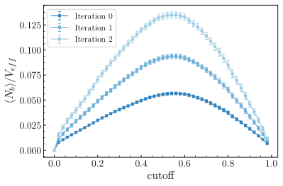
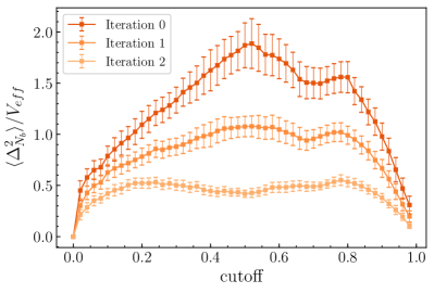
Figure 18: $\langle N_{b}\rangle$ and $\langle\Delta_{N_{b}}^{2}\rangle$ vs. grayscale cutoff value for 500 randomly chosen images from the CIFAR-10 dataset.

Immediately we see that there is no identifiable low temperature phase, and that for cutoff values near both $0$ and $1$, we obtain images which are mostly empty, similar to the high temperature configurations obtained from the worm algorithm. This suggests that there is no such notion of criticality (as characterized by the abrupt transition from a low to high temperature phase) like we found for the two-dimensional Ising model.

References

- (1) S.-H. Li and L. Wang, 1802.02840 .
- (2) C. Bény, arXiv:1301.3124 .
- (3) P. Mehta and D. J. Schwab, arXiv:1410.3831 .
- Foreman et al. (2018) S. Foreman, J. Giedt, Y. Meurice, and J. Unmuth-Yockey, Proceedings, 35th International Symposium on Lattice Field Theory (Lattice 2017): Granada, Spain, June 18-24, 2017, EPJ Web Conf. 175, 11025 (2018), arXiv:1710.02079 [hep-lat] .
- (5) S. Bradde and W. Bialek, Journal of Statistical Physics 167, 462, arXiv:1610.09733 .
- Carrasquilla and Melko (2017) J. Carrasquilla and R. G. Melko, Nature Physics 13, 431 (2017), arXiv:1605.01735 [cond-mat.str-el] .
- Wang (2016) L. Wang, Phys. Rev. B 94, 195105 (2016).
- Hu et al. (2017) W. Hu, R. R. P. Singh, and R. T. Scalettar, Phys. Rev. E 95, 062122 (2017), arXiv:1704.00080 [cond-mat.stat-mech] .
- Wetzel (2017) S. J. Wetzel, Phys. Rev. E 96, 022140 (2017), arXiv:1703.02435 [cond-mat.stat-mech] .
- Levin and Nave (2007) M. Levin and C. P. Nave, Phys. Rev. Lett. 99, 120601 (2007).
- Gu et al. (2009) Z.-C. Gu, M. Levin, B. Swingle, and X.-G. Wen, Phys. Rev. B 79, 085118 (2009).
- Xie et al. (2012) Z. Y. Xie, J. Chen, M. P. Qin, J. W. Zhu, L. P. Yang, and T. Xiang, Phys. Rev. B 86, 045139 (2012).
- Meurice (2013) Y. Meurice, Phys. Rev. B87, 064422 (2013), arXiv:1211.3675 [hep-lat] .
- Liu et al. (2013) Y. Liu, Y. Meurice, M. P. Qin, J. Unmuth-Yockey, T. Xiang, Z. Y. Xie, J. F. Yu, and H. Zou, Phys. Rev. D88, 056005 (2013), arXiv:1307.6543 [hep-lat] .
- Denbleyker et al. (2014) A. Denbleyker, Y. Liu, Y. Meurice, M. P. Qin, T. Xiang, Z. Y. Xie, J. F. Yu, and H. Zou, Phys. Rev. D89, 016008 (2014), arXiv:1309.6623 [hep-lat] .
- Yu et al. (2014) J. F. Yu, Z. Y. Xie, Y. Meurice, Y. Liu, A. Denbleyker, H. Zou, M. P. Qin, and J. Chen, Phys. Rev. E89, 013308 (2014), arXiv:1309.4963 [cond-mat.stat-mech] .
- Savit (1980) R. Savit, Rev. Mod. Phys. 52, 453 (1980).
- Prokof’ev and Svistunov (2001) N. Prokof’ev and B. Svistunov, Phys. Rev. Lett. 87, 160601 (2001).
- Enßlin and Frommert (2011) T. A. Enßlin and M. Frommert, Phys. Rev. D 83, 105014 (2011).
- Prokof’ev (2004) N. Prokof’ev, “Worm algorithm for ising model,” (2004), ”http://mcwa.csi.cuny.edu/umass/izing/Ising_text.pdf”.
- Bishop (2006) C. M. Bishop, Pattern recognition and machine learning (Springer, New York, 2006).
- Shanahan et al. (2018) P. E. Shanahan, D. Trewartha, and W. Detmold, Phys. Rev. D97, 094506 (2018), arXiv:1801.05784 [hep-lat] .
- Swendsen and Wang (1987) R. H. Swendsen and J.-S. Wang, Phys. Rev. Lett. 58, 86 (1987).
- Kaufman (1949) B. Kaufman, Phys. Rev. 76, 1232 (1949).
- Krizhevsky and Hinton (2009) A. Krizhevsky and G. Hinton, Master’s thesis, Department of Computer Science, University of Toronto (2009).