Tensor chain and constraints in tensor networks

Abstract

This paper accompanies with our recent work on quantum error correction (QEC) and entanglement spectrum (ES) in tensor networks (arXiv:1806.05007). We propose a general framework for planar tensor network state with tensor constraints as a model for $AdS_{3}/CFT_{2}$ correspondence, which could be viewed as a generalization of hyperinvariant tensor networks recently proposed by Evenbly. We elaborate our proposal on tensor chains in a tensor network by tiling $H^{2}$ space and provide a diagrammatical description for general multi-tensor constraints in terms of tensor chains, which forms a generalized greedy algorithm. The behavior of tensor chains under the action of greedy algorithm is investigated in detail. In particular, for a given set of tensor constraints, a critically protected (CP) tensor chain can be figured out and evaluated by its average reduced interior angle. We classify tensor networks according to their ability of QEC and the flatness of ES. The corresponding geometric description of critical protection over the hyperbolic space is also given.

I Introduction

Tensor network as a powerful tool for building the ground state of a many-body system has been greatly investigated in recent years Vidal:2007hda . One remarkable feature of tensor network states is the intuitive description of quantum entanglement among local degrees of freedom. For a subsystem composed of some uncontracted edges in a tensor network, its entanglement entropy is vividly bounded by the minimal cuts disconnecting this subsystem and its complementarity. This scenario can be viewed as the discretized description of Ryu-Takayanagi (RT) formula in holographic approach Ryu:2006bv . Inspired by this, people find that a holographic space can emerge from entanglement renormalization of a many-body system Swingle:2009bg ; Swingle:2012wq . It has further been conjectured in VanRaamsdonk:2010pw and Maldacena:2001kr that the classical connectivity of spacetime arises by entangling the degrees of freedom in two components. As a bridge between quantum entanglement and the structure of spacetime, tensor networks have been providing a practical framework for exploring the emergence of spacetime in the context of gauge/gravity duality Nozaki:2012zj ; Qi:2013caa .

Another property of entanglement enjoyed by holographic duality is quantum error correction (QEC) Schumacher:1996dy . Based on sub system duality, operators in the bulk can be reconstructed by the operators supported on a sub system of the boundary Hamilton:2006az ; Dong:2016eik ; Harlow:2018fse ; Cotler:2017erl . In other words, there are subspaces of the Hilbert space in the bulk which can still be reconstructed even if an amount of information on the boundary is erased Mintun:2015qda ; Freivogel:2016zsb ; Harlow:2016vwg ; Almheiri:2014lwa . Great progress has also been made in the realization of QEC by virtue of tensor networks Pastawski:2015qua ; Freivogel:2016zsb ; Mintun:2015qda ; Bhattacharyya:2016hbx ; Hayden:2016cfa ; Qi:2018shh . In this framework, sub system duality is reflected by the isometry between two sub Hilbert spaces associated with sub tensor networks.

The above properties of entanglement have been addressed in various tensor networks, including the multiscale entanglement renormalization ansatz (MERA) Swingle:2009bg ; Vidal:2007hda , perfect tensor networks Pastawski:2015qua ; Yang:2015uoa , random tensor networks Hayden:2016cfa ; Han:2017uco ; Bhattacharyya:2016hbx ; Qi:2018shh ; Chirco:2017wgl , hyperinvariant tensor networks Evenbly:2017htn , as well as spin networks Han:2016xmb .

Currently it is still a key issue whether tensor networks, or what kind of tensor networks could produce all the aspects of holography in the context of AdS/CFT correspondence. Taking $AdS_{3}$/$CFT_{2}$ as an example, we pick up some important properties that a tensor network is desired to possess.

• Such a tensor network is a discretization of 2-dimensional hyperbolic space ($H^{2}$ space), which is a time slice of an $AdS_{3}$ spacetime in global coordinate system. Correspondingly, the tensor network is endowed with a symmetry described by a discrete subgroup of $SL(2,R)$, which is the isometry of $H^{2}$ space.

• Such a tensor network respects RT formula and the entanglement entropy is characterized by a logarithmic law. Moreover, the entanglement spectrum (ES) of the ground state should be non-flat such that one can reproduce the Cardy-Calabrese formula of Renyi entropy for a $CFT_{2}$ with large central charge $c$, namely Calabrese:2004eu ; Calabrese:2009qy

  $$S_{n}(A)=\left(1+\frac{1}{n}\right)\frac{c}{6}\ln l_{A},$$ (1)

  where $A$ is a spatial interval on the boundary and $l_{A}$ is its length with the unit of UV cutoff.

• Such a tensor network has the function of QEC as AdS spacetime enjoys.

• Such a tensor network can reproduce the behavior of Green’s function in AdS₃/CFT₂.

Of course, all these properties may not be independent of one another.

One candidate for capturing above holographic features of AdS is hyperinvariant tensor networks, recently proposed by Evenbly in Evenbly:2017htn . It is composed of identical polygons by uniformly tiling hyperbolic space. The key idea is to impose constraints on the product of multiple tensors to form isometric mappings. It turns out that this sort of networks may combine the advantages of multiscale entanglement renormalization ansatz (MERA) Vidal:2007hda ; Swingle:2009bg ; Swingle:2012wq ; Kim:2016wby ; Bao:2015uaa which is characterized by non-flat ES and the network composed of perfect tensorsPastawski:2015qua ; Yang:2015uoa ; Donnelly:2016qqt which is usually endowed with the function of QEC.

But one key issue arises in this approach. That is, what kind of multi-tensor constraints could endow such features to a given tensor networks? or more quantitatively, is there any criteria to justify the ability of QEC and the non-flatness of ES for a given tensor networks with multi-tensor constraints? In Ling:2018qec we have provided affirmative answers to these issues with the proposal for critical protection on tensor chains. In this paper we intend to elaborate our proposal and present the detailed analysis on tensor chains and constraints in tensor networks and prove the statements on the classification of tensor networks in Ling:2018qec .

We organize the paper as follows. In next section we will propose a generalized framework for the tensor networks with multi-tensor constraints in the tiling of $H^{2}$ space. To classify different types of multi-tensor constraints efficiently and describe the behavior of tensor contractions during the evaluation of ES, we introduce the notion of tensor chain to describe the contraction of tensor products. Moreover, we will introduce a quantity, called the average reduced interior angle, to characterize the geometric structure of CP chain. Based on this structure we will introduce the concept of critical protection in Section III, which should be viewed as the core concept in our paper, because it plays an essential role in measuring the quality of QEC as well as the non-flatness of ES in a quantitative manner. As the first consequence, we will immediately see that once the ES becomes non-flat under the multi-tensor constraints as proposed in Evenbly:2017htn , then the ability of QEC from bulk to boundary has to be weakened. Among this sort of networks, we find that most of the perfect tensor networks as the limit case have the strongest ability of QEC, while they are always accompanied by a flat ES. Therefore, in order to construct tensor networks with a non-flat ES as AdS spacetime, one has to pay the price of sacrificing the ability of QEC. All above investigation is based on a tensor networks embedded into $H^{2}$ space which can be viewed as a discretization of the hyperbolic geometry. Correspondingly, we may also describe QEC and ES over the geometry of $H^{2}$ directly, which involves the notion of geodesics and the curves of constant curvature, etc. We present the description based on $H^{2}$ geometry in Section IV and the relevant backgrounds are given in Appendix A. Keep going on, to intuitively understand the role of critical protection in the evaluation of QEC and ES, in Section V we present some specific examples of tensor networks and demonstrate how the realization of QEC could be reflected by the structure of CP tensor chain, and how the flatness of ES can be reflected by the region of critical protection. Moreover, we develop a generalized description of greedy algorithm by imposing multi-tensor constraints on tensor chains. After that we classify tensor networks with constraints by their properties of QEC and ES. We firstly study the relation between CP and QEC in Section VI, presenting a criteria for the existence of QEC, and then focus on the relation between CP and ES in Section VII, with detailed proofs of the propositions on various bounds for the flatness of ES. Section VIII is the conclusion and outlook.

II Tensor chains in a tensor network

In this section we will present a general framework for tensor networks based on the tiling of hyperbolic space. We define a notion of tensor chain whose skeleton forms a polyline in a network. Associated with each tensor chain, the reduced interior angle can be defined, which in some sense could be viewed as the discrete description of the curvature of the ployline.

II.1 Tiling of $H^{2}$ space

In the global coordinate system of $AdS_{3}$ spacetime, the isochronous surface is a $H^{2}$ space

$$ds^{2}=L^{2}(d\rho^{2}+\cosh^{2}\rho d\tau^{2}),$$ (2)

where $L$ is the radius of $H^{2}$ geometry, the unique dimensional quantity introduced in this paper. So we are free to set $L=1$.

Firstly, we intend to discretize $H^{2}$ space in a uniform version, which can be realized by the tiling of $H^{2}$ space with identical polygons. Consider many identical polygons composed of $b$ edges in a $2$ dimensional surface, then put them together by gluing their edges such that $a$ edges share the same node. We call such discretization as the $\{b,a\}$ tiling of $H^{2}$ space. In a space with negative curvature, because the sum of interior angles of a triangle is less than $2\pi$, one can realize a $\{b,a\}$ tiling of $H^{2}$ space only if

$$\frac{1}{a}+\frac{1}{b}<\frac{1}{2}.$$ (3)

Obviously, $a\geq 3,b\geq 3$.

When a tiling of $H^{2}$ is specified by $\{b,a\}$, the geometry is determined (up to the radius $L$). We call the polygon with $b$ edges as the elementary polygon, while the union of several elementary polygons as a composite polygon. The length of each edge of the elementary polygon is

$$P=2\text{ arccosh}\left(\frac{\cos\left(\frac{\pi}{b}\right)}{\sin\left(\frac{\pi}{a}\right)}\right).$$ (4)

II.2 Tensor networks with $\{b,a\}$ tiling

Now we construct a tensor network based on a $\{b,a\}$ tiling. Associated with each node, we assign a rank-a tensor $T$, each index of which is specified to an edge jointed at the node respectively. The elements of the tensor $T$ are denoted as $T^{i_{1}i_{2}\cdots i_{a}}$, where all indexes have the same dimension $d$ and $d>1$. Associated with each edge, we also assign a rank-2 tensor $E$, whose elements are $E_{i_{1}i_{2}}$. We call the above indexes associated with tensors $T$ and $E$ as basic indexes, which are labelled by lowercase letters. As examples, two tensor networks with $\left\{7,3\right\}$ tiling and $\left\{4,5\right\}$ tiling are illustrated in Fig.1, respectively.

Because of the rotational invariance of $H^{2}$ space, we further demand that the indexes of tensor $T$ and $E$ have cyclic symmetry

$$T^{i_{1}i_{2}\cdots i_{a}}=T^{i_{2}i_{3}\cdots i_{a}i_{1}},\quad E_{i_{1}i_{2}}=E_{i_{2}i_{1}}.$$ (5)

In this paper, we adopt the convention that the index of tensor $T$ can be lowered by contracting it with a tensor $E$

$$T_{j_{1}}{}^{i_{2}\cdots i_{a}}\equiv\sum_{i_{1}}E_{j_{1}i_{1}}T^{i_{1}i_{2}\cdots i_{a}}.$$ (6)

Correspondingly, the edge connecting two nodes represents the index contraction of two tensors $T$ by a tensor $E$, namely,

$$\sum_{i_{1}j_{1}}T^{i_{1}i_{2}\cdots i_{a}}E_{i_{1}j_{1}}T^{j_{1}j_{2}\cdots j_{a}}=\sum_{i_{1}}T^{i_{1}i_{2}\cdots i_{a}}T_{i_{1}}{}^{j_{2}\cdots j_{a}}.$$ (7)

Therefore, given a tensor network with $\left\{b,a\right\}$ tiling, we can define a quantum state $\Psi$ consisting of two sorts of tensors $T$ and $E$ by tensor products and contractions. For later convenience, we require that for a tensor network state $\Psi$, all the indexes of tensors $T$ (with full upper indexes) should be contracted and those uncontracted indexes should only belong to tensors $E$, as shown in Fig.1.

A tensor network $\Psi$ can define a state $\left|\Psi\right\rangle$ in the Hilbert space on those uncontracted edges. In this paper, we will investigate the algorithms of QEC and the entanglement of $\Psi$ by manipulating tensor networks.

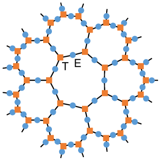
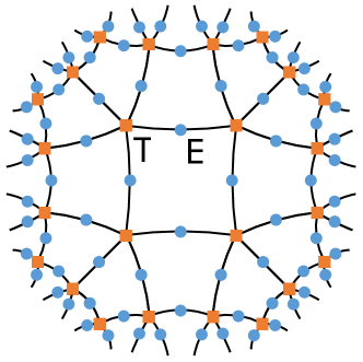
Figure 1: Two tensor networks with (a) $\left\{7,3\right\}$ tiling and (b) $\left\{4,5\right\}$ tiling, where a tensor $T$ is marked by an orange square while a tensor $E$ is marked by a blue dot. Only finite layers are plotted. For convenience, all the tensors $T$ and $E$ will not be manifestly displayed in the latter figures of tensor network except necessary.

II.3 Tensor chain

Given a tensor network by the $\{b,a\}$ tiling, we intend to introduce a notion of tensor chain to depict the product structure of multi-tensors with index contractions, which will be convenient for us to impose a tensor constraint and quantitatively describe its geometric properties. Firstly, in order to define a tensor chain in an efficient way, we adopt a compact form to denote a single tensor $T$ of rank-$a$ which is subject to rotational symmetry. We divide all its indexes into four groups in order and label each group with an abstract index, which is called collected index and labelled by a capital letter. Then the component of $T$ can be generally written as $T^{ABCD}$. For instance, for a tensor $T^{i_{1}i_{2}\cdots i_{5}}$ with $5$ indexes, we may collect them as $i_{1}i_{2}=A,\,i_{3}=B,\,i_{4}=C,\,i_{5}=D$ or $i_{1}i_{2}=A,\,i_{3}i_{4}=B,\,i_{5}=C,\,\varnothing=D$, while the collection $i_{1}i_{2}=A,\,i_{3}=C,\,i_{4}=B,\,i_{5}=D$ is prohibited. Furthermore, those collected indexes may also be lowered by tensor $E$, such as

$$T_{A^{\prime}}{}^{BCD}\equiv T_{i_{1}^{\prime}i_{2}^{\prime}}{}^{i_{3}i_{4}i_{5}}\equiv\sum_{i_{1}i_{2}}E_{i_{1}^{\prime}i_{1}}E_{i_{2}^{\prime}i_{2}}T^{i_{1}i_{2}\cdots i_{5}}\equiv\sum_{A}E_{A^{\prime}A}T^{ABCD},$$ (8)

where $i_{1}^{\prime}i_{2}^{\prime}=A^{\prime},\,i_{1}i_{2}=A,\,i_{3}=B,\,i_{4}=C,\,i_{5}=D$ and $E_{A^{\prime}A}\equiv E_{i_{1}^{\prime}i_{1}}E_{i_{2}^{\prime}i_{2}}$. We further define $\#(A)$ as the number of basic indexes in a collected index $A$. For example, in the above collection, $\#(A)=2$ and $\#(B)=1$.

Now we can construct a tensor chain $M$ by contracting $k$ tensors $T$ with tensors $E$

$$M^{A}_{B}=M^{A_{1}A_{2}\cdots A_{k}}_{B_{1}B_{2}\cdots B_{k}}=\sum_{C_{1}C_{2}\cdots C_{k},C_{1}=C_{k+1}}\prod_{i=1}^{k}T^{A_{i}C_{i}}{}_{B_{i}C_{i+1}}$$ (9)

where $A=A_{1}A_{2}\cdots A_{k}$ and $B=B_{1}B_{2}\cdots B_{k}$ are uncontracted indexes, while $C_{1},C_{2},\cdots C_{k}$ are specified as the indexes which are contracted in the chain. Moreover, since each tensor $T$ occupies a node in the tiling, we call $k$ the number of nodes in tensor chain $M$ as well. The sum index $i$ in (9) runs from $1$ to $k$, counting the number of nodes in $M$. Alternatively, a tensor chain $M$ can be viewed as a mapping from the Hilbert space on uncontracted indexes $A$ to the Hilbert space on uncontracted indexes $B$.

Obviously, in a $\{b,a\}$ tiling any two nodes are only possibly connected by single edge, otherwise they are not connected directly. Thus, here we only consider tensor chain with $\#(C_{i})=1$ for $i=2,3,\cdots,k$. Furthermore, if $\#(C_{1})=\#(C_{k+1})=1$, then we call $M$ as a closed tensor chain; if $\#(C_{1})=\#(C_{k})=0$, we call $M$ as an open tensor chain. Two typical samples of tensor chain are illustrated in Fig.2.

Since a diagram of tensor chain can be specified by the number of uncontracted edges in the tensor product, we propose a notation $\begin{bmatrix}[0.5]m_{1}&m_{2}&\cdots&m_{k}\\ n_{1}&n_{2}&\cdots&n_{k}\end{bmatrix}$ to denote an open tensor chain $M$ with elements $M^{A_{1}A_{2}\cdots A_{k}}_{B_{1}B_{2}\cdots B_{k}}$, where $m_{i}\equiv\#(A_{i})$ and $n_{i}\equiv\#(B_{i})$. Obviously, we have

$$m_{i},n_{i}\geq 0,\quad m_{i}+n_{i}=a-2+\delta_{i1}+\delta_{i,k},\quad i=1,2,\cdots,k.$$ (10)

Similarly, we use $\begin{pmatrix}[0.5]m_{1}&m_{2}&\cdots&m_{k}\\ n_{1}&n_{2}&\cdots&n_{k}\end{pmatrix}$ to denote a closed tensor chain with

$$m_{i},n_{i}\geq 0,\quad m_{i}+n_{i}=a-2,\quad i=1,2,\cdots,k.$$ (11)

Since one can reconstruct $m_{i}$ from $n_{i}$ or vice versa according to (10)(11), some time for convenience we abbreviate either $m_{i}$ or $n_{i}$ to $*$. For instance, $\begin{bmatrix}[0.5]*&*&\cdots&*\\ n_{1}&n_{2}&\cdots&n_{k}\end{bmatrix}\equiv\begin{bmatrix}[0.5]m_{1}&m_{2}&\cdots&m_{k}\\ *&*&\cdots&*\end{bmatrix}\equiv\begin{bmatrix}[0.5]m_{1}&m_{2}&\cdots&m_{k}\\ n_{1}&n_{2}&\cdots&n_{k}\end{bmatrix}$ with (10) and $\begin{pmatrix}[0.5]*&*&\cdots&*\\ n_{1}&n_{2}&\cdots&n_{k}\end{pmatrix}\equiv\begin{pmatrix}[0.5]m_{1}&m_{2}&\cdots&m_{k}\\ *&*&\cdots&*\end{pmatrix}\equiv\begin{pmatrix}[0.5]m_{1}&m_{2}&\cdots&m_{k}\\ n_{1}&n_{2}&\cdots&n_{k}\end{pmatrix}$ with (11).

We provide the following definition to describe some relations among tensor chains.

Definition 1.

Given a tensor network with $\{b,a\}$ tiling and an open tensor chain $M=\begin{bmatrix}[0.5]m_{1}&m_{2}&\cdots&m_{k}\\ *&*&\cdots&*\end{bmatrix}$, we define its sub tensor chain $M_{p,q}$ as $\begin{bmatrix}[0.5]m_{p}&m_{p+1}&\cdots&m_{q}\\ *&*&\cdots&*\end{bmatrix}$ for $1\leq p\leq q\leq k$. We say $M^{\prime}\sqsubseteq M$ if $M^{\prime}$ is a sub tensor chain of $M$. Furthermore, we say an open tensor chain $\begin{bmatrix}[0.5]m_{1}^{\prime}&m_{2}^{\prime}&\cdots&m_{l}^{\prime}\\ *&*&\cdots&*\end{bmatrix}\preceq M$ where $1\leq l\leq k$, if $\exists p\in\left\{1,2,\cdots,k-l+1\right\}$ s.t. $m_{i}^{\prime}\leq m_{p+i-1}$ for $i\in\left\{1,l\right\}$ and $m_{i}^{\prime}=m_{p+i-1}$ for $1<i<l$.

Given a closed tensor chain $M=\begin{pmatrix}[0.5]m_{1}&m_{2}&\cdots&m_{k}\\ *&*&\cdots&*\end{pmatrix}$, we define its sub tensor chain $M_{p,q}$ for $1\leq p\leq k$, $1\leq q\leq k$ as $\begin{bmatrix}[0.5]m_{1}^{\prime\prime}&m_{2}^{\prime\prime}&\cdots&m_{l}^{\prime\prime}\\ *&*&\cdots&*\end{bmatrix}$ where $m_{i}^{\prime\prime}=m_{p+i-1\text{ mod }k}$ for $1\leq i\leq l$ and $1\leq l=q-p+1<k$. We say $M^{\prime}\sqsubseteq M$ if $M^{\prime}$ is a sub tensor chain of $M$. Furthermore, we say an open tensor chain $\begin{bmatrix}[0.5]m_{1}^{\prime}&m_{2}^{\prime}&\cdots&m_{l}^{\prime}\\ *&*&\cdots&*\end{bmatrix}\preceq M$ where $1\leq l<k$ if $\exists p$ s.t. $m_{i}^{\prime}\leq m_{p+i-1\text{ mod }k}$ for $i=\left\{1,l\right\}$ and $m_{i}^{\prime}=m_{p+i-1\text{ mod }k}$ for $1<i<l$.

For example, in $\left\{4,5\right\}$ tiling, $\begin{bmatrix}[0.5]2&1\\ 2&3\end{bmatrix}\sqsubseteq\begin{bmatrix}[0.5]2&1&2\\ 2&2&2\end{bmatrix}$ and $\begin{bmatrix}[0.5]2&1&1\\ 2&2&3\end{bmatrix}\preceq\begin{bmatrix}[0.5]2&1&2\\ 2&2&2\end{bmatrix}$.

We always require that the subscripts $p,q$ in $M_{p,q}$ belong to integers and satisfy $1\leq p\leq q\leq k$, where $k$ is the number of nodes in $M$.

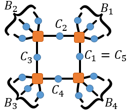
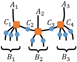
Figure 2: A closed tensor chain $\begin{pmatrix}[0.5]0&0&0&0\\ 3&3&3&3\end{pmatrix}$ and an open tensor chain $\begin{bmatrix}[0.5]1&1&1\\ 3&2&3\end{bmatrix}$.

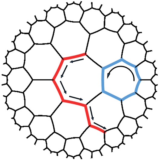
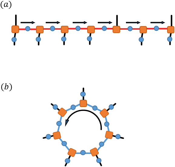
Figure 3: Two polylines and their tensor chains in a tensor network with $\left\{7,3\right\}$ tiling. The tensor chain of red polyline is shown in (a) and the tensor chain of blue polyline is shown in (b).

II.4 The reduced interior angle

When a tensor chain is embedded into a tensor network in $H^{2}$ space, its skeleton can be marked by a directed polyline concisely, as shown in Fig.3. Along the direction of the polyline, we require that the sequence number of nodes increases and the edges on the left (right) hand side of the polyline are always associated with the upper (lower) indexes of the tensor chain. For a closed tensor chain, conventionally the direction of the closed polyline is specified to be anticlockwise, so the inward or left-handed (outward or right-handed) edges of the polyline are associated with the upper (lower) indexes of the tensor chain. We remark that a closed polyline with clockwise direction can be analyzed in parallel, with the requirement that its inward (outward) edges are associated with the lower (upper) indexes.

The curvature of a polyline at the $i$th node can be captured by its interior angle $\theta_{i}$, which is defined as the angle on the left hand side of the polyline and is a multiple of $2\pi/a$. We further define the reduced interior angle as $s_{i}=\theta_{i}/\frac{2\pi}{a}$, which is an integer. Obviously, the reduced interior angle is related to the number of upper edges at each node and we intend to give the following definition.

Definition 2.

For a closed tensor chain $M=\begin{pmatrix}[0.5]m_{1}&m_{2}&\cdots&m_{k}\\ *&*&\cdots&*\end{pmatrix}$, the reduced interior angle of the i-th tensor is $s_{i}=m_{i}+1$. For an open tensor chain $M=\begin{bmatrix}[0.5]m_{1}&m_{2}&\cdots&m_{k}\\ *&*&\cdots&*\end{bmatrix}$, the reduced interior angles are $s_{i}=m_{i}+1-\delta_{i1}$.

For later convenience, we further introduce several quantities based on reduced interior angles to evaluate the curvature of a tensor chain $M$. Specially, we define the prime tensor chain, which is the core notion for the construction of the algebra of tensor constraints in next subsection.

Definition 3.

Given a tensor chain $M$ with $k$ nodes, the average reduced interior angle $\kappa(M)$ is defined as

$$\kappa(M)=\frac{1}{k}\sum_{i=1}^{k}s_{i}.$$ (12)

The sub reduced interior angle $\kappa_{p,q}(M)$ from the p-th tensor to the q-th tensor is defined as

$$\kappa_{p,q}(M)=\kappa(M_{p,q}),\quad 1\leq p\leq q\leq k,$$ (13)

and the maximal reduced interior angle $\kappa_{p,q}(M)$ is defined as

$$\kappa_{max}(M)=\max_{p,q}\kappa_{p,q}(M).$$ (14)

Definition 4.

Given an open tensor chain $M$ with finite $k$ nodes, when that $\kappa_{p,q}(M)=\kappa_{max}(M)$ if and only if $p=1$ and $q=k$, then we say tensor chain $M$ is prime.

Based on above definitions, we have following theorems for tensor chains.

Theorem 1.

Given two tensor chains $M$ and $M^{\prime}$, if $M\preceq M^{\prime}$, then $\kappa_{max}(M)\leq\kappa_{max}(M^{\prime})$.

Theorem 2.

Given a tensor chains $M$ and a prime tensor chain $M^{\prime}$, if $M\preceq M^{\prime}$ but $M\neq M^{\prime}$, then $\kappa_{max}(M)<\kappa(M^{\prime})$.

Theorem 3.

The uniqueness theorem of prime tensor chain. Given a $\{b,a\}$ tiling and a rational number

$$\kappa\in\left[1,\frac{a}{2}\right],$$ (15)

the prime tensor chain $M$ with $\kappa(M)=\kappa$ exists and is unique. Furthermore, if $\kappa=u/v$ where $u$ and $v$ are coprime integers, then $M=\begin{bmatrix}[0.5]m_{1}&m_{2}&\cdots&m_{v}\\ n_{1}&n_{2}&\cdots&n_{v}\end{bmatrix}$ with

$$m_{i}=[i\kappa]-[(i-1)\kappa]-1+\delta_{i1},$$ (16)

where $[x]$ is the floor function. So, $M$ has reversal symmetry, namely

$$m_{i}=m_{v-i+1}.$$ (17)

The reduced interior angles of $M$ are given by

$$s_{i}=[i\kappa]-[(i-1)\kappa].$$ (18)

Proof.

Set a prime tensor chain $M=\begin{bmatrix}[0.5]m_{1}&m_{2}&\cdots&m_{k}\\ n_{1}&n_{2}&\cdots&n_{k}\end{bmatrix}$ satisfying $\kappa(M)=\kappa$. Then, for $l=1,2,\cdots,k-1$,

$$\frac{1}{k}\sum_{i=1}^{k}m_{i}+k-1 = \kappa,$$ (19)

$$\frac{1}{l}\sum_{i=1}^{l}m_{i}+l-1 < \kappa,$$ (20)

$$\frac{1}{k-l}\sum_{i=1}^{k-l}m_{i}+k-l-1 < \kappa.$$ (21)

On one hand, from (19)(20)(21), one has

$$\sum_{i=1}^{l}m_{i}-1<l(\kappa-1)<\sum_{i=1}^{l}m_{i}.$$ (22)

Then

$$l(\kappa-1)\notin\mathbb{Z}\Rightarrow l/v\notin\mathbb{Z},\quad l=1,2,\cdots,k-1.$$ (23)

Thus

$$v\geq k.$$ (24)

On the other hand, from (20), one has

$$k\kappa\in\mathbb{Z}\Rightarrow k/v\in\mathbb{Z}.$$ (25)

Combining above two statements, we have

$$k=v.$$ (26)

From (20)(22), one has

$$\sum_{i=1}^{l}m_{i}=[l(\kappa-1)]+1,\quad l=1,2,\cdots,v.$$ (27)

So

$$m_{l}=\sum_{i=1}^{l}m_{i}-\sum_{i=1}^{l-1}m_{i}=[l\kappa]-[(l-1)\kappa]-1,\quad l=2,3,\cdots,v.$$ (28)

Specially, when $l=1$,

$$m_{1}=[1*\kappa]-[0*\kappa]-1+1.$$ (29)

In summary, we have proved (16). Moreover, using identities

$$\begin{split}[-x]&=-[x]-1+\delta_{x,[x]},\\ [x+n]&=[x]+n,\quad n\in\mathbb{Z},\end{split}$$ (30)

we can derive (17). Then according to Definition 2, we have (18). At last, from (18) we find

$$m_{1}=[\kappa]\text{ or }[\kappa]-1.$$ (31)

It leads to the conclusion that conditions in (10) can always be satisfied if we require (15). So the prime tensor chain exists and is unique. ∎

Theorem 4.

For a tensor chain $M$, $\exists$ unique prime tensor chain $M^{\prime}$ satisfying $M^{\prime}\sqsubseteq M$ and $\kappa(M^{\prime})=\kappa_{max}(M)$.

Proof.

$\exists p,q$ s.t. $\kappa_{p,q}(M)=\kappa_{max}(M)$ and $\kappa_{p^{\prime},q^{\prime}}(M)<\kappa_{max}(M)$, $\forall p^{\prime},q^{\prime}$ satisfying $p<p^{\prime}\leq q^{\prime}\leq q$ or $p\leq p^{\prime}\leq q^{\prime}<q$. Then $M^{\prime}=M_{p,q}$ is prime, whose $\kappa(M^{\prime})=\kappa_{p,q}(M)=\kappa_{max}(M)$. Because of Theorem 3, $M^{\prime}$ is unique. ∎

III Tensor constraints and Critically Protected (CP) tensor chains

In this section we propose a notion of critical protection to describe the behavior of tensor networks under the contractions of tensor product which are subject to tensor constraints.

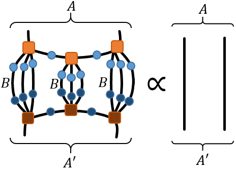
Figure 4: Multi-tensor constraint constructed by open tensor chain $\begin{bmatrix}[0.5]1&0&1\\ 3&3&3\end{bmatrix}$.

III.1 Tensor constraint

The notion of tensor chain provides us a convenient way to describe a general constraint on the product of tensors $T$ and $E$, which plays an essential role in pushing operators through nodes or edges in network in the context of QEC. Usually we impose the constraint requiring that some contraction of tensors should be proportional to an isometry. Of course the contraction of tensors may or may not form a tensor chain. Here for simplicity, we only consider imposing tensor constraints on tensor chains which can be concisely written as

$$\sum_{B}M^{A}_{B}(M_{B}^{A^{\prime}})^{*}\propto\delta^{AA^{\prime}},$$ (32)

where $M=\begin{bmatrix}[0.5]m_{1}&m_{2}&\cdots&m_{k}\\ n_{1}&n_{2}&\cdots&n_{k}\end{bmatrix}$ is an open tensor chain with $n_{i}$ to be the number of edges that are contracted with its conjugate tensor at the $i$th node, as illustrated in Fig.4. Notice that the contraction on two lower indexes $B$ in (32) implies that it involves in $\#(B)$ contractions of $\sum_{j}E_{ij}(E_{jk})^{*}$. For convenience, in the remainder of this paper, when we say a tensor constraint $M$, we actually refer to the constraint in terms of tensor chain $M$ which is subject to (32). Obviously, a non-trivial constraint $M$ requires $\sum_{i=1}^{k}m_{i}\geq 1$. Moreover, an isometry can be realized only if the number of degrees of freedom in $A$ is less than or equal to that in $B$, namely

$$\sum_{i=1}^{k}m_{i}=\#(A)\leq\#(B)=\sum_{i=1}^{k}n_{i}.$$ (33)

Thus, any non-trivial tensor constraint $M$ should satisfy

$$\kappa(M)\in\left[1,\frac{a}{2}\right].$$ (34)

One may immediately find that for a set of tensor constraints some of them may not be logically independent. In general, there are four fundamental operations to derive new constraints from given tensor constraints, which can be listed as follows.

Reversal

If $\begin{bmatrix}[0.5]m_{1}&m_{2}&\cdots&m_{k}\\ n_{1}&n_{2}&\cdots&n_{k}\end{bmatrix}$ is a tensor constraint, then $\begin{bmatrix}[0.5]m_{k}&m_{k-1}&\cdots&m_{1}\\ n_{k}&n_{k-1}&\cdots&n_{1}\end{bmatrix}$ is a tensor constraint as well.

Contraction

If $\begin{bmatrix}[0.5]m_{1}&m_{2}&\cdots&m_{k}\\ n_{1}&n_{2}&\cdots&n_{k}\end{bmatrix}$ is a tensor constraint, then $\begin{bmatrix}[0.5]m_{1}-1&m_{2}&\cdots&m_{k}\\ n_{1}+1&n_{2}&\cdots&n_{k}\end{bmatrix}$ is a tensor constraint as well.

Reduction

If $\begin{bmatrix}[0.5]m_{1}&m_{2}&\cdots&m_{k}\\ n_{1}&n_{2}&\cdots&n_{k}\end{bmatrix}$ and $\begin{bmatrix}[0.5]*&*&\cdots&*\\ n_{p}&n_{p+1}&\cdots&n_{q}\end{bmatrix}$ are tensor constraints, where $2\leq p\leq q\leq k$, then $\begin{bmatrix}[0.5]m_{1}&m_{2}&\cdots&m_{p-1}\\ *&*&\cdots&*\end{bmatrix}$ is a tensor constraint as well.

Combination

If $\begin{bmatrix}[0.5]*&*&\cdots&*\\ n_{1}&n_{2}&\cdots&n_{k}\end{bmatrix}$ and $\begin{bmatrix}[0.5]m_{1}^{\prime}&m_{2}^{\prime}&\cdots&m_{l}^{\prime}\\ *&*&\cdots&*\end{bmatrix}$ are tensor constraints, then
$\begin{bmatrix}[0.5]*&*&\cdots&*&m_{1}^{\prime}&m_{2}^{\prime}&\cdots&m_{l}^{\prime}\\ n_{1}&n_{2}&\cdots&n_{k}&*&*&\cdots&*\end{bmatrix}$ is a tensor constraint as well.

As an example, we demonstrate the derivation of new constraints by contraction and reduction in Fig.5.

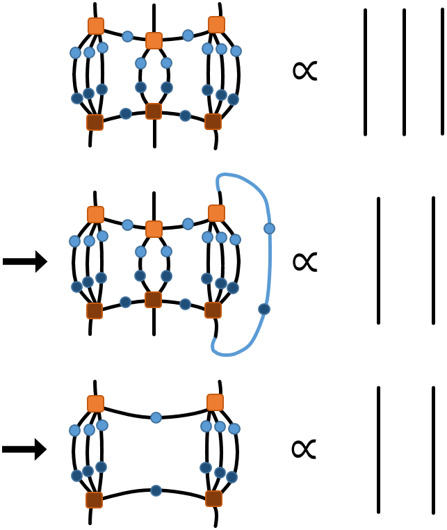
Figure 5: Logical derivation of tensor constraint $\begin{bmatrix}[0.5]1&1\\ 3&3\end{bmatrix}$ from $\left\{\begin{bmatrix}[0.5]1\\ 4\end{bmatrix},\begin{bmatrix}[0.5]1&1&1\\ 3&2&3\end{bmatrix}\right\}$.

We remark that the strength of a tensor constraint $M$ can be quantified by its maximal reduced interior angle $\kappa_{max}(M)$. By comparing $\kappa_{max}$ of new derived constraints with those of original constraints, we have the following theorem.

Theorem 5.

Any tensor constraint $M^{\prime\prime}$ derived from $M$ and $M^{\prime}$ through above ways satisfies

$$\kappa_{max}(M^{\prime\prime})\leq\max\left(\kappa_{max}\left(M\right),\kappa_{max}\left(M^{\prime}\right)\right).$$ (35)

where $M=\begin{bmatrix}[0.5]m_{1}&m_{2}&\cdots&m_{k}\\ n_{1}&n_{2}&\cdots&n_{k}\end{bmatrix},M^{\prime}=\begin{bmatrix}[0.5]m_{1}^{\prime}&m_{2}^{\prime}&\cdots&m_{l}^{\prime}\\ n_{1}^{\prime}&n_{2}^{\prime}&\cdots&n_{l}^{\prime}\end{bmatrix}$.

Proof.

For reversal, $\kappa_{max}(M^{\prime\prime})=\kappa_{max}(M)$, then we have (35).
For contraction and reduction, $M^{\prime\prime}\preceq M$. Thanks to Theorem 1, we have (35).
For combination, $\exists p,q$ s.t. $\kappa_{p,q}(M^{\prime\prime})=\kappa_{max}(M^{\prime\prime})$. In the case of $q\leq k$ or $k<p$, similarly, we have (35). In the case of $p\leq k<q$, we observe that

$$1+\frac{\sum_{i=p}^{k}m_{i}-1}{k-p+1} \leq \kappa_{max}(M),$$ (36)

$$1+\frac{\sum_{i=1}^{k-q}m_{i}^{\prime}-1}{q-k} \leq \kappa_{max}(M^{\prime}),$$ (37)

which leads to

$$\sum_{i=p}^{k}m_{i}+\sum_{i=1}^{q-k}m_{i}^{\prime}\leq 2+(\kappa_{max}(M)-1)(k-p+1)+(\kappa_{max}(M^{\prime})-1)(q-k).$$ (38)

So,

$$\begin{split}\kappa_{p,q}(M^{\prime\prime})&=1+\frac{\sum_{i=p}^{k}m_{i}+\sum_{i=1}^{q-k}m_{i}^{\prime}-2}{q-p+1}\\ &\leq\frac{k-p+1}{q-p+1}\kappa_{max}(M)+\frac{q-k}{q-p+1}\kappa_{max}(M^{\prime})\\ &\leq\max\left(\kappa_{max}\left(M\right),\kappa_{max}\left(M^{\prime}\right)\right).\end{split}$$ (39)

In summary, we have (35). ∎

Next we intend to study a set of tensor constraints with the form

$$S=\left\{M_{s},M_{1},M_{2},\cdots\right\},$$ (40)

where $M_{s}=\begin{bmatrix}[0.5]1\\ a-1\end{bmatrix}$ is called step tensor chain and other tensor constraints are not specified. Step tensor chain has the minimal average reduce interior angle $\kappa(M_{s})=1$. Generally, those tensor constraints in $S$ may not be mutually independent. With the help of step tensor chain, we have the following theorem for the relation of tensor constraints.

Theorem 6.

Any tensor constraint $M$ satisfying $M\preceq M^{\prime}$ can be derived from $S=\left\{M_{s},M^{\prime}\right\}$.

For any general set of tensor constraints, we can find a unique set of tensor constraints $S_{c}$ which is logically equivalent to $S$ and only contains two elements

$$S_{c}=\left\{M_{s},M_{t}\right\}.$$ (41)

$S_{c}$ is called central set. $M_{t}$ is called top tensor chain, which should be prime and satisfy the condition (34). The equivalence between $S$ and $S_{c}$ require $\kappa(M_{t})=\max\limits_{M\in S}\kappa_{max}(M)$, as proved in Theorem (8). Without loss of generality, we will only consider central set $S_{c}$ hereinafter.

Thanks to Theorem 3, given a $\left\{b,a\right\}$ tiling, we have a one-to-one mapping between all the possible top tensor chains $M_{t}$ and the rational numbers in $\left[1,\frac{a}{2}\right]$. Thus, we have classified all the general sets of tensor constraints with the form in (40) by the rational number $\kappa(M_{t})\in[1,\frac{a}{2}]$. Given a $\kappa(M_{t})$, with the use of (16), we can directly construct top tensor chain $M_{t}$ as well as those tensor chains $M$ satisfying $M\preceq M_{t}$.

Theorem 7.

Given a central set $S_{c}=\left\{M_{s},M_{t}\right\}$, we define a set $S_{D}=\left\{M|\kappa_{max}(M)\leq\kappa(M_{t})\right\}$. A tensor constraint $M$ can be derived from $S_{c}$ if and only if $M\in S_{D}$.

Proof.

Let $M_{t}=\begin{bmatrix}[0.5]m_{1}&m_{2}&\cdots&m_{k}\\ n_{1}&n_{2}&\cdots&n_{k}\end{bmatrix},M=\begin{bmatrix}[0.5]m_{1}^{\prime}&m_{2}^{\prime}&\cdots&m_{k^{\prime}}^{\prime}\\ n_{1}^{\prime}&n_{2}^{\prime}&\cdots&n_{k^{\prime}}^{\prime}\end{bmatrix}$. We denote the proposition that $M$ can be derived from $S_{c}$ as $P1$.

If $P1$ is true, thanks to Theorem 2 and Theorem 5, we have $\kappa_{max}(M)\leq\kappa(M_{t})$, thus $M\in S_{D}$.

Next we will apply the method of induction on $k^{\prime}$ to prove that if $\kappa_{max}(M)\leq\kappa(M_{t})$ then $P1$ is true.

Firstly, for the simplest case with $k^{\prime}=1$, $\kappa_{max}(M)=m_{1}^{\prime}$ is an integer. Because of Theorem 3, $m_{1}=[\kappa(M_{t})]$. Then $\kappa_{max}(M)\leq\kappa(M_{t})\Rightarrow m_{1}^{\prime}\leq m_{1}\Rightarrow M\preceq M_{t}$. Because of Theorem 6, $P1$ is true.

Now assume that when $1\leq k^{\prime}<l$ $P1$ is true, we are going to prove that for $k^{\prime}=l$, $P1$ is also true.

At current stage, the length of tensor chain $M$, namely $l$, could be either longer or shorter than the length of $M_{t}$, namely $k$. In either case, we will compare the number of upper basic indexes at each node within the parts with the same length, $\min(k,l)$. To describe the difference of this part in two tensor chains, it is convenient to define the proposition that $\exists j\in\left\{1,2,\cdots,\min(k,l)\right\}$ s.t. $m_{j}^{\prime}\neq m_{j}$ as $P2$. Then for $k^{\prime}=l$, We split the situation into the following three cases.

1. $P2$ is false and $l\leq k$. It means that the tensor chain $M$ is shorter or has equal length, and has the same number of upper basic indexes as $M_{t}$ at each node. Then obviously one has $M\sqsubseteq M_{t}$, so $P1$ is true.

2. $P2$ is false and $l>k$. It means the tensor chain $M$ has the same number of upper basic indexes as $M_{t}$ at first $k$ nodes but it is longer. One can pick out the extra part of $M$ by setting $M^{\prime}=\begin{bmatrix}[0.5]m_{k+1}^{\prime}+1&m_{k+2}^{\prime}&\cdots&m_{l}^{\prime}\\ *&*&\cdots&*\end{bmatrix}$. For $p>1$, one can easily derive that $\kappa_{p,q}(M^{\prime})=\kappa_{p+k,q+k}(M)\leq\kappa_{max}(M)\leq\kappa(M_{t})$. While for $p=1$, one has $\kappa_{1,q}(M^{\prime})=\frac{1}{q}\left\{(k+q)\kappa_{1,k+q}(M)-k\kappa(M_{t})\right\}\leq\frac{1}{q}\left\{(k+q)\kappa(M_{t})-k\kappa(M_{t})\right\}=\kappa(M_{t})$. So $\kappa_{max}(M^{\prime})\leq\kappa(M_{t})$. Because of the assumption of induction and $l-k<l$, $M^{\prime}$ can be derived from $S_{c}$. Now since $M$ can be derived from $M^{\prime}$ and $M_{t}$ by reversal and combination, $P1$ must be true.

3. $P2$ is true. It means the number of upper basic indexes at some nodes are different in two tensor chains. Set the minimal $j$ satisfying $m_{j}^{\prime}\neq m_{j}$ as $r$. If $m_{r}^{\prime}>m_{r}$, then $m_{r}^{\prime}\geq m_{r}+1$. So $\kappa_{1,r}(M)\geq\frac{1}{r}\left(m_{1}+\cdots+m_{r}+1+r-1\right)=\frac{1}{r}\left\{\sum_{i=1}^{r}([i\kappa(M_{t})]-[(i-1)\kappa(M_{t})]-1+\delta_{i1})+r\right\}=\frac{1}{r}\left([r\kappa(M_{t})]+1\right)>\kappa(M_{t})$, where (16) is used. It is contradictory to the condition $\kappa_{max}(M)\leq\kappa(M_{t})$. So only $m_{r}^{\prime}<m_{r}$ is possible. Now we set $M^{\prime}=\begin{bmatrix}[0.5]m_{1}^{\prime}&m_{2}^{\prime}&\cdots&m_{r-1}^{\prime}&m_{r}^{\prime}+1\\ *&*&\cdots&*&*\end{bmatrix}$ and $M^{\prime\prime}=\begin{bmatrix}[0.5]m_{r+1}^{\prime}&m_{r+2}^{\prime}&\cdots&m_{l}^{\prime}\\ *&*&\cdots&*\end{bmatrix}$ (If $r=1$, set $M^{\prime}=\begin{bmatrix}[0.5]m_{1}^{\prime}+1\\ *\end{bmatrix}$), then $M^{\prime}\preceq M_{t}$ and $M^{\prime\prime}\preceq M$. So $M^{\prime}$ can be derived from $S_{c}$ and $\kappa_{max}(M^{\prime\prime})\leq\kappa(M)$. Because of the assumption of induction and $l-r<l$, $M^{\prime\prime}$ can be derived from $S_{c}$ as well. Since $M$ can be derived from $M^{\prime}$ and $M^{\prime\prime}$ by combination, $P1$ is true.

In conclusion, $P1$ is true when $\kappa_{max}(M)\leq\kappa(M_{t})$. ∎

Theorem 8.

Any general set of tensor constraints $S=\left\{M_{s},M_{1},M_{2},\cdots\right\}$ is logically equivalent to a unique central set of tensor constraints $S_{c}=\left\{M_{s},M_{t}\right\}$, where $M_{t}$ is specified by $\kappa(M_{t})=\max\limits_{M\in S}\kappa_{max}(M)$.

Proof.

$\exists M\in S$ s.t. $\kappa_{max}(M)=\max\limits_{M^{\prime}\in S}\kappa_{max}(M^{\prime})$. Because of Theorem 4, $\exists$ unique prime tensor chain $M_{t}$ satisfying $M_{t}\sqsubseteq M$ and $\kappa(M_{t})=\kappa_{max}(M)$. Because of Theorem 6, $S\Rightarrow\left\{M_{s},M\right\}\Rightarrow S_{c}$ and $\kappa(M_{t})=\max\limits_{M\in S}\kappa_{max}(M)$.

On the other hand, because of Theorem 7, $S_{c}\Rightarrow\left\{M_{s},M\right\}$, $\forall M\in S$. Thus, $S_{c}\Rightarrow S$.

Thus, $\exists$ unique prime $M_{t}$ s.t. $S\Leftrightarrow S_{c}$ and $\kappa(M_{t})=\max\limits_{M\in S}\kappa_{max}(M)$. ∎

One may ask whether there always exist tensor $T$ and tensor $E$ satisfying the tensor constraints $S_{c}$. We do not have a general proof about the existence here. Nevertheless, for some specific tensor constraints, we can actually solve them by constructing specific tensors indeed. Some examples are demonstrated in Appendix B and see more in Ling:2018qec .

III.2 Protection

In this subsection we describe the behavior of tensor chains under the action of tensor constraints. For this purpose we first give the following definitions.

Definition 5.

The transpose of an open tensor chain $M=\begin{bmatrix}[0.5]m_{1}&m_{2}&\cdots&m_{k}\\ n_{1}&n_{2}&\cdots&n_{k}\end{bmatrix}$ is $M^{T}=\begin{bmatrix}[0.5]n_{1}&n_{2}&\cdots&n_{k}\\ m_{1}&m_{2}&\cdots&m_{k}\end{bmatrix}$. The transpose of a closed tensor chain $M=\begin{pmatrix}[0.5]m_{1}&m_{2}&\cdots&m_{k}\\ n_{1}&n_{2}&\cdots&n_{k}\end{pmatrix}$ is $M^{T}=\begin{pmatrix}[0.5]n_{1}&n_{2}&\cdots&n_{k}\\ m_{1}&m_{2}&\cdots&m_{k}\end{pmatrix}$.

Definition 6.

Given a set of tensor constraints $S_{c}=\left\{M_{s},M_{t}\right\}$, say a tensor chain $M$ is unprotected, if $\exists M^{\prime}\in S_{D}$ such that $M^{\prime T}\sqsubseteq M^{T}$. Otherwise, we say that $M$ is protected.

The notion of protection can be intuitively understood as following. If we find such $M^{\prime}$ in $S_{D}$ satisfying $M^{\prime T}\sqsubseteq M^{T}$, then the contraction

$$\sum_{B_{i}B_{i+1}\cdots B_{j}}M^{A_{1}A_{2}\cdots A_{k}}_{B_{1}B_{2}\cdots B_{k}}\left(M^{\prime}{}_{B_{i}B_{i+1}\cdots B_{j}}^{D_{i}D_{i+1}\cdots D_{j}}\right)^{*},\quad 1\leq i\leq j\leq k$$ (42)

can be simplified under the constraint $S_{c}=\left\{M_{s},M_{t}\right\}$. Diagrammatically, the tensor chain $M$ becomes disconnected under the contraction with the tensor chain $M^{\prime*}$, as illustrated in Fig.6. In other words, when we say a tensor chain is protected, it means that one can not factorize it by contracting its lower indexes with any $M\in S_{D}$ derived from $S_{c}$. Actually, the condition in Definition 6, namely “$\exists M^{\prime}\in S_{D}$”, can be simplified as “$\exists M^{\prime}\preceq M_{t}$”.

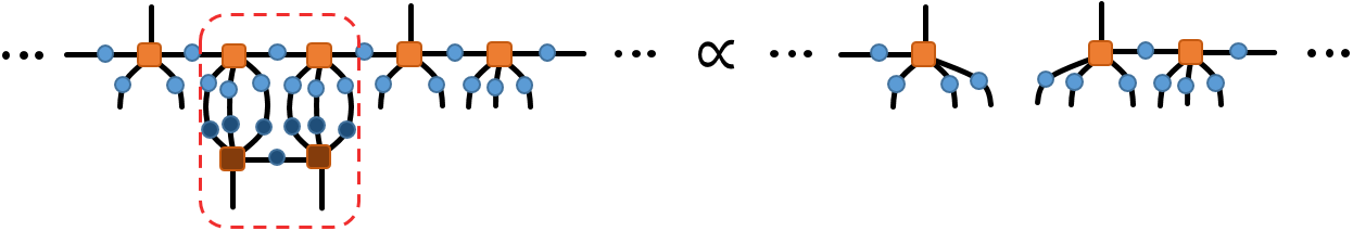
Figure 6: A unprotected tensor chain $\begin{pmatrix}[0.5]\cdots&1&0&0&1&0&\cdots\\ \cdots&2&3&3&2&3&\cdots\end{pmatrix}$ becomes disconnected when contracting it with the conjugation of $\begin{bmatrix}[0.5]1&1\\ 3&3\end{bmatrix}$ in $S_{c}=\left\{\begin{bmatrix}[0.5]1\\ 4\end{bmatrix},\begin{bmatrix}[0.5]1&1\\ 3&3\end{bmatrix}\right\}$.

III.3 CP tensor chains

In this subsection we point out that given a tiling and $S_{c}$, there exists a tensor chain which is critically protected. We notice that whether a tensor chain $M$ is protected or not can be reflected by the value of interior angles, which roughly speaking measures the curvature of the skeleton of the tensor chain. Specifically, the larger is $\kappa_{max}(M^{T})$, the easier it is for $M$ to become unprotected. Therefore, there is a critical value for $\kappa$ at which tensor chain is critically protected.

Definition 7.

Given an open tensor chain $M=\begin{bmatrix}[0.5]m_{1}&m_{2}&\cdots&m_{k-1}&m_{k}\\ n_{1}&n_{2}&\cdots&n_{k-1}&n_{k}\end{bmatrix}$, we can define a periodic tensor chain by joining infinitely many $M$s as

$$M_{period}=\left(\begin{array}[]{cccccccccccc}\cdots&m_{1}-1&m_{2}&\cdots&m_{k-1}&m_{k}&m_{1}-1&m_{2}&\cdots&m_{k-1}&m_{k}&\cdots\\ \cdots&n_{1}&n_{2}&\cdots&n_{k-1}&n_{k}-1&n_{1}&n_{2}&\cdots&n_{k-1}&n_{k}-1&\cdots\end{array}\right)$$ (43)

with a loop body $\begin{pmatrix}[0.5]m_{1}-1&m_{2}&m_{3}&\cdots&m_{k}\\ n_{1}&n_{2}&n_{3}&\cdots&n_{k}-1\end{pmatrix}$ . $k$ is called the period of $M_{period}$.

Obviously, $\kappa(M_{period})=\kappa(M)$.

Definition 8.

Given a tiling and the set $S_{c}$, we define the critically protected (CP) tensor chain $M_{c}$ as the periodic tensor chain generated by $M_{t}$. We further define the CP reduced interior angle as $\kappa_{c}=\kappa(M_{c})=\kappa(M_{t})$.

We demonstrate the construction of $M_{c}$ with an example in Fig.7.

The exact meaning of critical protection is characterized by the following theorem.

Theorem 9.

With a given $\{b,a\}$ tiling and a given $S_{c}$, an open tensor chain $M=\begin{bmatrix}[0.5]*&*&\cdots&*\\ n_{1}&n_{2}&\cdots&n_{k}\end{bmatrix}$ is unprotected if and only if $\exists p,q$ satisfying $1\leq p\leq q\leq k$ such that

$$\sum_{i=p}^{q}(a-1-n_{i})\leq(q-p+1)\kappa_{c}-1.$$ (44)

A closed tensor chain $M=\begin{pmatrix}[0.5]*&*&\cdots&*\\ n_{1}&n_{2}&\cdots&n_{k}\end{pmatrix}$ is unprotected if and only if $\exists p,h$ satisfying $h\leq k$ such that

$$\sum_{i=1}^{h}(a-1-n_{(p+i-1)\mod k})\leq h\kappa_{c}-1.$$ (45)

Proof.

We will present the proof for the case of open tensor chain in detail and claim that it can be applied to closed tensor chain in parallel. The main difference will be mentioned in the end of proof.

We first prove the proposition: if $\exists p,q$ satisfying $1\leq p\leq q\leq k$ such that (44) is true, then $M$ is unprotected. Without lose of generality, we start with the assumption that $\not\exists p^{\prime},q^{\prime}$ with $p<p^{\prime}\leq q^{\prime}\leq q$ or $p\leq p^{\prime}\leq q^{\prime}<q$ satisfying $\sum_{i=p^{\prime}}^{q^{\prime}}(a-1-n_{i})\leq(q^{\prime}-p^{\prime}+1)\kappa_{c}-1$. Otherwise, we just replace $p,q$ by $p^{\prime},q^{\prime}$.

Let $h=q-p+1$ and $x_{i}=a-1-n_{i}$, $\forall i$. There are two cases:

1. If $h=1$, then $a-n_{p}\leq\kappa_{c}\Rightarrow a-n_{p}\leq[\kappa_{c}]$. Because of (16), $\begin{bmatrix}[0.5]a-n_{p}\\ n_{p}\end{bmatrix}\preceq\begin{bmatrix}[0.5][\kappa_{c}]\\ a-[\kappa_{c}]\end{bmatrix}\preceq M_{t}$. We know $\begin{bmatrix}[0.5]a-n_{p}\\ n_{p}\end{bmatrix}^{T}\sqsubseteq M^{T}$, then $M$ is unprotected.

2. If $h\geq 2$, then $\forall l\in\{1,2,\cdots,h-1\}$, we have

$$\sum_{i=p}^{p+l-1}x_{i}>l\kappa_{c}-1,$$ (46)

$$\sum_{i=p+l}^{q}x_{i}>(h-l)\kappa_{c}-1.$$ (47)

From (44)(46)(47), we have

$$l\kappa_{c}-1<\sum_{i=p}^{p+l-1}x_{i}<l\kappa_{c} \Rightarrow \sum_{i=p}^{p+l-1}x_{i}=[l\kappa_{c}],$$ (48)

$$h\kappa_{c}-2<\sum_{i=p}^{q}x_{i}\leq h\kappa_{c}-1 \Rightarrow \sum_{i=p}^{q}x_{i}=[h\kappa_{c}]-1.$$ (49)

Let the rational number $\kappa_{c}=u/v$, where $u,v\in\mathbb{N^{+}}$ and $u,v$ are coprime. From (48), we know $l\kappa_{c}\notin\mathbb{Z}$, then $l/v\not\in\mathbb{Z},\forall l\in\{1,2,...,h-1\}$. Thus $v\geq h$. From (48)(49), we have $x_{l+p-1}=[l\kappa_{c}]-[(l-1)\kappa_{c}]-\delta_{lh}$. We define $M^{\prime}=\begin{bmatrix}[0.5]m_{1}^{\prime}&m_{2}^{\prime}&\cdots&m_{h}^{\prime}\\ n_{1}^{\prime}&n_{2}^{\prime}&\cdots&n_{h}^{\prime}\end{bmatrix}$ where $n_{i}^{\prime}=n_{i+p-1}$. So $M^{\prime T}\sqsubseteq M^{T}$ and $m_{i}^{\prime}=[i\kappa_{c}]-[(i-1)\kappa_{c}]-\delta_{i1}-1$. Comparing $M^{\prime}$ with (16), we have $M^{\prime}\preceq M_{t}$ such that $M$ is unprotected.

Now we prove the converse proposition: If $M$ is unprotected, then $\exists p,q$ satisfying $1\leq p\leq q\leq k$ such that (44) is satisfied. Suppose that the top tensor chain $M_{t}=\begin{bmatrix}[0.5]m_{1}^{\prime}&m_{2}^{\prime}&\cdots&m_{v}^{\prime}\\ n_{1}^{\prime}&n_{2}^{\prime}&\cdots&n_{v}^{\prime}\end{bmatrix}$, and $M$ is unprotected when its tensors from the $p$th to the $q$th are acted on by a tensor constraint $M^{\prime}$. Since $M^{\prime T}\sqsubseteq M^{T}$ and $M^{\prime}\preceq M_{t}$, $\exists c,d$ satisfying $1\leq c\leq d\leq v$ and $d-c+1=q-p+1=h$ such that $x_{p+l-1}\leq m_{c+l-1}^{\prime}+1-\delta_{l1}-\delta_{lh}$, $\forall l\in\{1,2,\cdots,h\}$. By using (16), we further have

$$\begin{split}\sum_{i=p}^{q}x_{i}&\leq h-2+\sum_{i=c}^{d}m_{i}^{\prime}\\ &=h-2+\sum_{i=c}^{d}\left([i\kappa_{c}]-[(i-1)\kappa_{c}]-1+\delta_{i1}\right)\\ &=[d\kappa_{c}]-[(c-1)\kappa_{c}]-2+\delta_{c1}\\ &=[d\kappa_{c}]+[(1-c)\kappa_{c}]-1\\ &\leq[h\kappa_{c}]-1\\ &\leq h\kappa_{c}-1,\end{split}$$ (50)

where (30) is used. So (44) is satisfied.

As far as closed tensor chain is concerned, the only difference is that it has cyclic symmetry with modular $k$, namely $\begin{pmatrix}[0.5]*&*&\cdots&*&*\\ n_{1}&n_{2}&\cdots&n_{k-1}&n_{k}\end{pmatrix}=\begin{pmatrix}[0.5]*&*&\cdots&*&*\\ n_{2}&n_{3}&\cdots&n_{k}&n_{1}\end{pmatrix}$, then above $x_{i}$ is nothing but reduced interior angles, namely $s_{i}=a-1-n_{i}=x_{i}$. The proposition can be proved with the same algebra. ∎

From above theorem, we claim that any tensor chain $M$ satisfying $M^{T}\preceq M_{c}^{T}$ is protected; while any tensor chain $M$ satisfying $M\preceq M_{c}$ and $M\neq M_{c}$ is unprotected.

Similarly, thanks to Theorem 3, we have a one-to-one mapping between CP tensor chain $M_{c}$ and CP reduced interior angle $\kappa_{c}$.

Critical protection characterizes the limit of mapping the information from one side (with upper indexes) to another side (with lower indexes) with full fidelity. So the physical correspondence of CP tensor chain is the maximal boundary of the region where the interior information can be mapped to the boundary without loss.

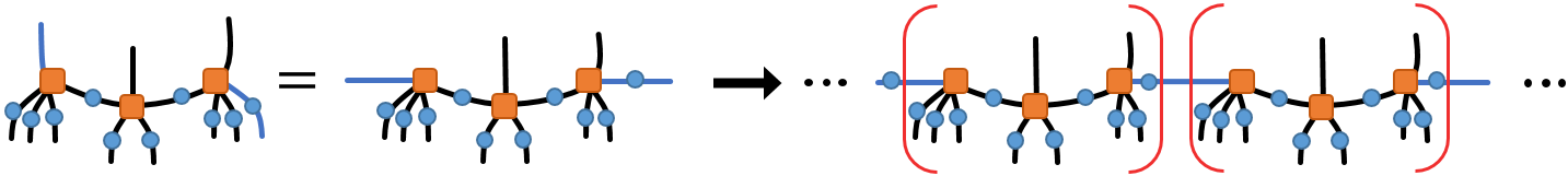
Figure 7: By using top tensor chain $\begin{bmatrix}[0.5]1&1&1\\ 3&2&3\end{bmatrix}$, we can define loop body $\begin{pmatrix}[0.5]0&1&1\\ 3&2&2\end{pmatrix}$ and construct a CP tensor chain $\begin{pmatrix}[0.5]\cdots&0&1&1&0&1&1&\cdots\\ \cdots&3&2&2&3&2&2&\cdots\end{pmatrix}$.

IV Geometric description

In this section we elaborate some geometric properties of the tensor network with $\{b,a\}$ tiling in $H^{2}$ space, which will be essential for us to provide a quantitative description for the QEC and ES in tensor networks. The isometry group of $H^{2}$ space is $SL(2,R)$. In $H^{2}$ space, the curves of constant curvature (CCC) include circles, hypercircles and horocircles, depending on their values of geodesic curvature. Geodesic is a kind of hypercircle . A brief review on $SL(2,R)$ and CCC is given in Appendix A.

IV.1 The curve of constant curvature corresponding to a periodic polyline

The $\left\{b,a\right\}$ tiling breaks the isometry group $SL(2,R)$ into a discrete subgroup $G_{\text{tiling}}$, which is the set of all transformations preserving the tiling. We are interested in two specific generators $V,S$ of $G_{\text{tiling}}$, where $V$ is the anticlockwise rotation around a node by an angle $2\pi/a$ and $S$ is the clockwise rotation around the midpoint of an edge linked to this node by $\pi$. $V,S$ should satisfy the following equations

$$S^{2}=V^{a}=(VS)^{b}=-1,$$ (51)

$$\mathrm{Tr}(S)=0,$$ (52)

$$\mathrm{Tr}(V)=2\cos(\pi/a),$$ (53)

$$\mathrm{Tr}(VS)=2\cos(\pi/b).$$ (54)

The solutions up to $SL(2,R)$ are

$$S=\left(\begin{array}[]{cc}0&-1\\ 1&0\\ \end{array}\right),\quad V=\left(\begin{array}[]{cc}\cos\left(\frac{\pi}{a}\right)&e^{\frac{P}{2}}\sin\left(\frac{\pi}{a}\right)\\ -e^{-\frac{P}{2}}\sin\left(\frac{\pi}{a}\right)&\cos\left(\frac{\pi}{a}\right)\\ \end{array}\right).$$ (55)

where length $P$ is given in (4).

Recall that a tensor chain can be embedded into a tensor network in $H^{2}$ space, as discussed at the beginning of Subsection III.1. Similarly, a periodic tensor chain can also be embedded, whose skeleton forms an endless and periodic polyline. When the scale of a chain is much greater than the period of a polyline, the roughness of the skeleton can be zoomed out such that it looks like a CCC in $H^{2}$ space, whose geodesic curvature $\lambda$ is a constant. In general, given the embedding of a periodic tensor chain, we can define a unique CCC corresponding to this chain by specific operation. Next we will firstly present the procedures to locate such a CCC and finally discuss some exceptional cases that such CCC could not be defined.

The periodic tensor chain $M$ can be constructed from an open tensor chain according to Definition 7. We choose a node of $M$ and number it by $i$. The loop body beginning at the $(i+1)$th node is $\begin{pmatrix}[0.5]m_{i+1}&m_{i+2}&\cdots&m_{i+k}\\ n_{i+1}&n_{i+2}&\cdots&n_{i+k}\end{pmatrix}$, where $k$ is the period of $M$. Now we choose the center of the rotation generated by $V$ as the $i$th node and the center of the rotation generated by $S$ as the midpoint of the edge between the $i$th node and the $(i+1)$th node. Then we further define a transformation preserving the structure of periodic polyline as

$$W=V^{s_{i+k}}SV^{s_{i+k-1}}S\cdots V^{s_{i+2}}SV^{s_{i+1}}S,\quad s_{j}=m_{j}+1,\quad\forall j,$$ (56)

which maps each period in the polyline to the next period along the direction of the polyline. Starting from a point $q$ in $H^{2}$ space, the set of all the points generated by $W^{n}$, namely $Q_{W}=\{W^{n}q|n\in\mathbb{Z}\}$, will be located on a CCC. When $|Q_{W}|\geq 3$, the CCC can be uniquely determined.

We are interested in the case that point $q$ is the midpoint of one edge with lower index in $M$. With some algebra we finally derive that the geodesic curvature $\lambda$ of this kind of CCC can be calculated by

$$\lambda^{2}=\frac{[\mathrm{Tr}(\pi_{q}W)]^{2}}{(\mathrm{Tr}W)^{2}+[\mathrm{Tr}(\pi_{q}W)]^{2}-4},$$ (57)

where $\pi_{q}$ is the matrix of clockwise rotation by angle $\pi$ around point $q$, which belongs to $SL(2,R)$. $\pi_{q}$ can be generated by the generators $V$ and $S$, according to the relative position between point $q$ and the $i$th node.

Obviously, different choices of point $q$ generate different CCCs and $\lambda$s. To determine the unique CCC corresponding to $M$, we remark that one just need to choose the point $q$ which minimizes $|\lambda-1|$ in (57). The process of generating CCC from a periodic tensor chain is illustrated in Fig.8.

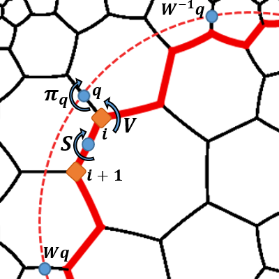
Figure 8: Generate a CCC from a periodic tensor chain with loop body $\begin{pmatrix}[0.5]0&1&0\\ 1&0&1\end{pmatrix}$ in $\left\{7,3\right\}$ tiling, where $\pi_{q}=V^{-1}SV$.

Once the CCC corresponding to a periodic tensor chain can be uniquely determined, the classification of CCC in (108) can be reformulated by the trace of $W$,

$$\begin{array}[]{ll}|\mathrm{Tr}(W)|<2,&\text{circle}\\ |\mathrm{Tr}(W)|=2,&\text{horocircle}\\ |\mathrm{Tr}(W)|>2,&\text{hypercircle}\\ \end{array}$$ (58)

From Theorem 3 and Definition 7, for a given rational number $\kappa\in[1,\frac{a}{2}]$, one can construct a unique prime tensor chain and its periodic tensor chain $M$ whose $\kappa(M)=\kappa$. As a result, one can further figure out the corresponding CCC as well as its geodesic curvature $\lambda$. So one can define a mapping from $\kappa$ to $\lambda$, as illustrated in Fig.9.

It may be noticed that not all the $\lambda$ can be inversely mapped to $\kappa$, because $\lambda$ is a positive number while $\kappa$ is a rational number. Nevertheless, horocircle, whose curvature $\lambda=1$, is a special kind of CCC in $H^{2}$ space. It corresponds to a closed tensor chain (closed polyline) in large radius limit. Furthermore, given a $\{b,a\}$ tiling, we can prove that the average reduced interior angle $\kappa_{h}$ of such a closed tensor chain is

$$\kappa_{h}=\frac{a}{2}-\frac{a-2}{2}\sqrt{\frac{ab-2a-2b}{ab-2a-2b+4}}.$$ (59)

Since this quantity plays a crucial role in classifying the tensor networks, we provide the detailed proof as follows.

Proof.

Horocircle is the limit of a circle with infinitely long radius in $H^{2}$ space. To construct the polyline corresponding to horocircle in a tensor network, we may consider the process of increasing the scale of a closed polyline. In a network with $\{b,a\}$ tiling, we consider a closed polyline $M$ with $k$ nodes and its total reduced interior angle is $l$. So the average reduced interior angle of $M$ is $\kappa=l/k$. Now it is helpful for us to plot the Poincare dual of the network with $\{b,a\}$ tiling, which is a network with $\{a,b\}$ tiling and all the nodes located at centers of dual polygons, as illustrated in Fig.10.

Given a polyline $M$, its outer adjoint polyline $M^{\prime}$ in Poincare dual network can be constructed step by step: (1) find out those elementary polygons in Poincare dual network whose center is located at the node of $M$; (2) pick out the edges of those polygons outside of $M$; (3) link those edges in order and then obtain a closed polyline which is just $M^{\prime}$.

The relation between $M$ and $M^{\prime}$ is illustrated in Fig.10. One can find that $M^{\prime}$ has $(a-1)k-l$ nodes and its total reduced interior angle is $ak-l$. Keep going on, one can find the outer adjoint polyline $M^{\prime\prime}$ of polyline $M^{\prime}$ will fall back into the network with $\{b,a\}$ tiling. Similarly, polyline $M^{\prime\prime}$ has $(b-1)((a-1)k-l)-ak+l$ nodes and its total reduced interior angle is $b((a-1)k-l)-ak+l$. So its average reduced interior angle is

$$\kappa^{\prime\prime}=\frac{b((a-1)k-l)-ak+l}{(b-1)((a-1)k-l)-ak+l}=\frac{(1-b)\kappa+(b-2)c_{1}(a-c_{1})}{(2-b)\kappa+ab-2a-b+1}\equiv f(\kappa),$$ (60)

where

$$c_{1}\equiv\frac{a}{2}-\frac{a-2}{2}\sqrt{\frac{ab-2a-2b}{ab-2a-2b+4}}.$$ (61)

The number of nodes enclosed by $M^{\prime\prime}$ is always more than that enclosed by $M$. Thus, if we begin with an elementary closed polyline with $b$ nodes and total reduced interior angle $b$ and continuously find the outer adjoint polyline, we will approach the polyline corresponding to a horocircle. Thus we have

$$\kappa_{h}=\lim_{n\to\infty}f^{n}(1),$$ (62)

where $f^{n}$ represents $f$ applied $n$ times. To evaluate above limit, we observe that

$$\frac{\kappa^{\prime\prime}-c_{1}}{\kappa^{\prime\prime}+c_{1}-a}=c_{2}\frac{\kappa-c_{1}}{\kappa+c_{1}-a},$$ (63)

where

$$c_{2}\equiv\frac{1-b-2c_{1}+bc_{1}}{1-b+(2-b)(c_{1}-a)},\quad 0<c_{2}<1.$$ (64)

Thus

$$\lim_{n\to\infty}\frac{f^{n}(1)-c_{1}}{f^{n}(1)+c_{1}-a}=0.$$ (65)

Since $f^{n}(1)$ must be finite, we finally have

$$\kappa_{h}=\lim_{n\to\infty}f^{n}(1)=c_{1}.$$ (66)

∎

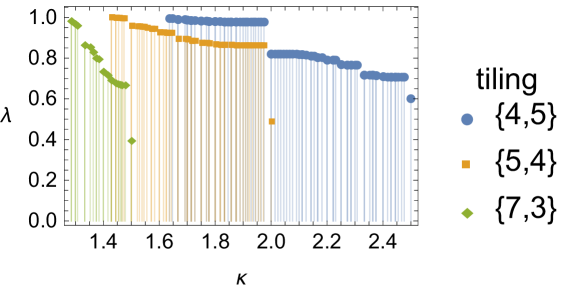
Figure 9: $\lambda$ as a function of $\kappa$ in different tilings, where only some rational numbers of $\kappa\in(\kappa_{h},\kappa_{0}]$ are shown.

Now we discuss some exceptional cases. The first case is $|Q_{W}|\leq 2$, namely the number of generated points less than two, so CCC can not be uniquely defined through the above process. The second case is that $M_{period}$ bends in an irregular way such that the embedding of periodic tensor chain may lead to a self-crossed polyline and no CCC could form, such as the $M_{period}$ with loop body $\begin{pmatrix}[0.5]1&1&1\\ 5&4&5\end{pmatrix}$ in the tensor network with $\left\{3,7\right\}$ tiling. Such two cases only happen for some $\kappa\in[1,\kappa_{h})$.

IV.2 CP curves

The CCC corresponding to a CP tensor chain is called CP curve, whose geodesic curvature is called CP curvature $\lambda_{c}$. CP curve is a generalization of the greedy geodesic in Pastawski:2015qua .

Given a tiling, CP curvature $\lambda_{c}$ and CP reduced interior angle $\kappa_{c}$ are inversely related to each other, as shown in Fig.9. If the CP tensor chain form a closed polyline, the CP curve is a circle, $\kappa_{c}<\kappa_{h}$ and $\lambda_{c}>1$. If the CP tensor chain form an open polyline which extends to the boundary, the CP curve is a hypercircle, $\kappa_{c}>\kappa_{h}$ and $\lambda_{c}<1$.

Roughly speaking, a periodic tensor chain is unprotected if its corresponding CCC has geodesic curvature $\lambda>\lambda_{c}$; while it is protected if the corresponding CCC has $\lambda<\lambda_{c}$ .

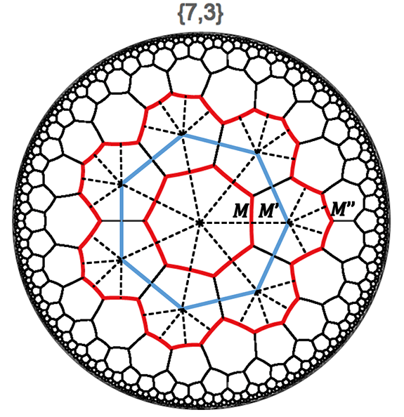
Figure 10: The minimal polyline $M$, the outer adjoint polyline $M^{\prime}$ of polyline $M$ and the outer adjoint polyline $M^{\prime\prime}$ of polyline $M^{\prime}$ in the network with $\left\{7,3\right\}$ tiling (solid line) and its Poincare dual (dashed line).

V Tensor networks and greedy algorithm

So far we have established a framework to describe tensor chains and tensor constraints. We will impose the central set $S_{c}$ to a tensor network in the sense that those constraints $M\in S_{D}$ derived from $S_{c}$ are valid, while those $M\notin S_{D}$ are not valid.

V.1 Tensor networks with $\left\{7,3\right\}$ tiling or $\left\{4,5\right\}$ tiling

Before analysing the role of critical protection in QEC and ES for general tensor networks, we construct some specific examples of tensor networks and provide an intuitive understanding on the notion of critical protection.

The structure of a tensor network with $\left\{7,3\right\}$ tiling is shown in Fig.1. According to (59), one has $\kappa_{h}=1.28$. We impose the central set $S_{c}=\left\{\begin{bmatrix}[0.5]1\\ 2\end{bmatrix},M_{t}\right\}$ for some typical $M_{t}$ and discuss the entanglement property of the tensor network. The structure of $M_{t}$, $M_{c}$, and the values of $\kappa_{c}$ and $\lambda_{c}$ are listed in Table.1. The corresponding diagrams of tensor constraints and CP tensor chains in the tiling are illustrated in Fig.14, 14, 14 and 14 respectively.

$M_{t}$	loop body of $M_{c}$	$\kappa_{c}$	$\lambda_{c}$	CP curve	QEC	ES
$\begin{bmatrix}[0.5]1\\ 2\end{bmatrix}$	$\begin{pmatrix}[0.5]0\\ 1\end{pmatrix}$	$1$	1.392	circle	N	non-flat
$\begin{bmatrix}[0.5]1&0&1\\ 1&1&1\\ \end{bmatrix}$	$\begin{pmatrix}[0.5]0&0&1\\ 1&1&0\end{pmatrix}$	$4/3$	0.869	hypercircle	Y	non-flat
$\begin{bmatrix}[0.5]1&0&1&0&1\\ 1&1&0&1&1\\ \end{bmatrix}$	$\begin{pmatrix}[0.5]0&0&1&0&1\\ 1&1&0&1&0\end{pmatrix}$	$7/5$	0.738	hypercircle	Y	mixed
$\begin{bmatrix}[0.5]1&1\\ 1&1\end{bmatrix}$	$\begin{pmatrix}[0.5]0&1\\ 1&0\end{pmatrix}$	$3/2$	0.398	hypercircle	Y	flat

Table 1: Properties about CP and entanglement for different tensor constraints in $\left\{7,3\right\}$ tiling.

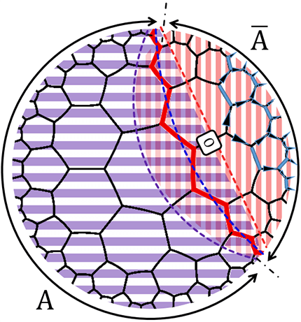
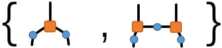
Figure 11: The tensor network with $\left\{7,3\right\}$ tiling and $S_{c}=\left\{\begin{bmatrix}[0.5]1\\ 2\end{bmatrix},\begin{bmatrix}[0.5]1&1\\ 1&1\end{bmatrix}\right\}$. The boundary is divided into two intervals $A$ and $\bar{A}$. Those tensors within the shaded region with purple (red) strips are absorbed by the greedy algorithm starting from $A$ ($\bar{A}$). The solid polyline in red denote a CP tensor chain. The red dashed curve is the CP curve (hypercircle); the blue dashed curve is its corresponding geodesic; the purple dashed curve is the reflection of CP curve with respect to the geodesic. An operator $O$ in the interior is pushed to the boundary.

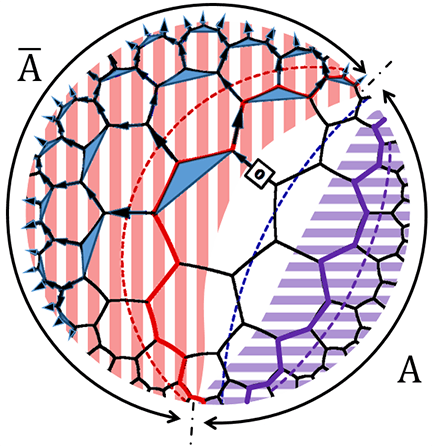
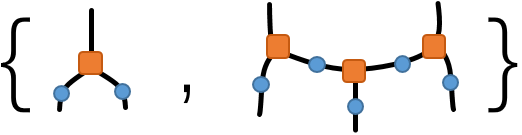
Figure 12: The tensor network with $\left\{7,3\right\}$ tiling and $S_{c}=\left\{\begin{bmatrix}[0.5]1\\ 2\end{bmatrix},\begin{bmatrix}[0.5]1&0&1\\ 1&1&1\\ \end{bmatrix}\right\}$. An operator is pushed to the boundary. The CP region is enclosed by two CP curves.

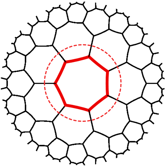
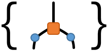
Figure 13: The tensor network with $\left\{7,3\right\}$ tiling and $S_{c}=\left\{\begin{bmatrix}[0.5]1\\ 2\end{bmatrix}\right\}$.

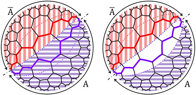
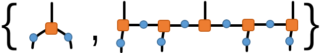
Figure 14: The tensor network with $\left\{7,3\right\}$ tiling and $S_{c}=\left\{\begin{bmatrix}[0.5]1\\ 2\end{bmatrix},\begin{bmatrix}[0.5]1&0&1&0&1\\ 1&1&0&1&1\\ \end{bmatrix}\right\}$.

In parallel, a tensor network with $\left\{4,5\right\}$ tiling is shown in Fig.1. In this case, one has $\kappa_{h}=1.63$. The entanglement properties of this tensor network with different top tensor chains are collected in Table.2. The corresponding diagrams of tensor constraints and the embedded CP tensor chains are plotted in Fig.18, 18, 18 and 18 respectively.

$M_{t}$	loop body of $M_{c}$	$\kappa_{c}$	$\lambda_{c}$	CP curve	QEC	ES
$\begin{bmatrix}[0.5]1\\ 4\end{bmatrix}$	$\begin{pmatrix}[0.5]0\\ 3\end{pmatrix}$	$1$	1.188	circle	N	non-flat
$\begin{bmatrix}[0.5]1&1&1\\ 3&2&3\\ \end{bmatrix}$	$\begin{pmatrix}[0.5]0&1&1\\ 3&2&2\end{pmatrix}$	$5/3$	0.994	hypercircle	Y	non-flat
$\begin{bmatrix}[0.5]2\\ 3\\ \end{bmatrix}$	$\begin{pmatrix}[0.5]1\\ 2\end{pmatrix}$	$2$	0.824	hypercircle	Y	mixed
$\begin{bmatrix}[0.5]2&2\\ 2&2\end{bmatrix}$	$\begin{pmatrix}[0.5]1&2\\ 2&1\end{pmatrix}$	$5/2$	0.604	hypercircle	Y	flat

Table 2: Properties about CP and entanglement for different tensor constraints in $\left\{4,5\right\}$ tiling.

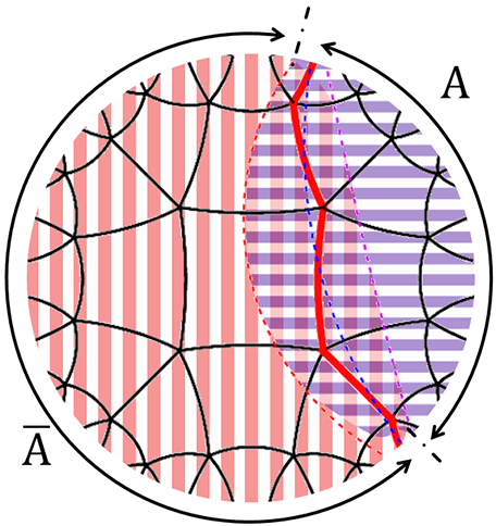
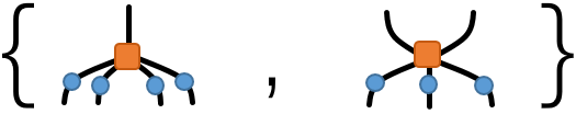
Figure 15: The tensor network with $\{4,5\}$ tiling and $S_{c}=\left\{\begin{bmatrix}[0.5]1\\ 4\end{bmatrix},\begin{bmatrix}[0.5]2&2\\ 2&2\end{bmatrix}\right\}$.

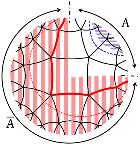
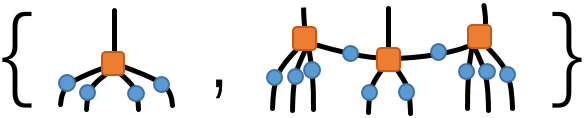
Figure 16: The tensor network with $\{4,5\}$ tiling and $S_{c}=\left\{\begin{bmatrix}[0.5]1\\ 4\end{bmatrix},\begin{bmatrix}[0.5]1&1&1\\ 3&2&3\end{bmatrix}\right\}$.

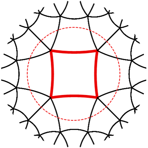
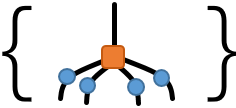
Figure 17: The tensor network with $\{4,5\}$ tiling and $S_{c}=\left\{\begin{bmatrix}[0.5]1\\ 4\end{bmatrix}\right\}$.

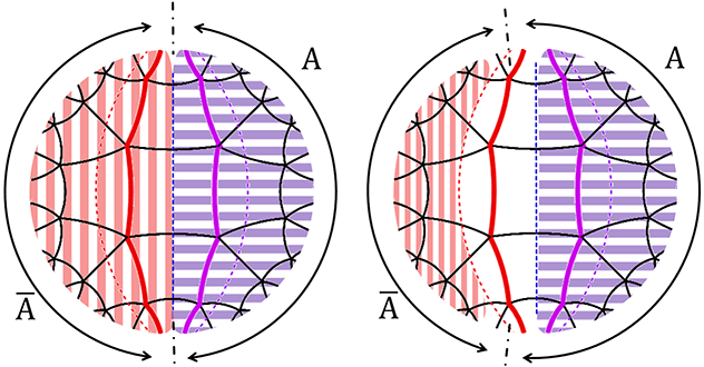
Figure 18: The tensor network with $\{4,5\}$ tiling and $S_{c}=\left\{\begin{bmatrix}[0.5]1\\ 4\end{bmatrix},\begin{bmatrix}[0.5]2\\ 3\end{bmatrix}\right\}$.

In above figures, we divide the boundary of the tensor network into two intervals $A$ and $\bar{A}$. The shaded region with different colors presents the effect of the greedy algorithm starting from $A$ and from $\bar{A}$ respectively, which will be further discussed in next subsection in detail. CP tensor chains are marked in each figure and its significance in greedy algorithm will be stressed as well. In next two sections, we will further take these figures as examples to disclose the relation between greedy algorithm and quantum error correction as well as entanglement spectrum.

V.2 Greedy algorithm on tensor chains

For a tensor network $\Psi$, we generalize the greedy algorithm in Pastawski:2015qua , based on the set $S_{D}$ derived from a central set $S_{c}$. After choosing an interval $A$ on the boundary, we consider a sequence of cuts $\left\{C_{n}\right\}$ and a sequence of sub tensor network $\left\{\Phi_{n}\right\}$, where each $C_{n}$ is bounded by $\partial A$ and each $\Phi_{n}$ consists of those tensors enclosed by $C_{n}$ and $A$, shaded with strips. So each $\Phi_{n}$ is a mapping from the Hilbert space on $C_{n}$ to the Hilbert space on $A$. Let $C_{1}=A$, then $\Phi_{1}$ is an identity. Next one figures out a tensor chain in the tiling which belongs to the set of $S_{D}$ and all of its lower indexes can be contracted with $\Phi_{n}$. Then $\Phi_{n+1}$ is constructed by absorbing such $M_{n}$ into $\Phi_{n}$. The greedy algorithm stops when no such tensor chain can be found. The way of iteration guarantees that each $\Phi_{n}$ is proportional to an isometry. As explained in Ling:2018qec , above greedy algorithm for a tensor network $\Psi$ is equivalent to the procedure of simplifying the contraction of tensor chains in (42), where $M$ is any tensor chain embedded in the tensor network $\Psi$.

To describe the process of greedy algorithm precisely, which is essential in the proofs for the properties of ES, we intend to extend the notion of protection to a directed cut in greedy algorithm.

One may notice that process of a greedy algorithm is not unique. Actually, one may have a lot of ways to arrange the sequence of absorbing tensor chains into the shaded region $\Phi_{n}$ such that during the course of greedy algorithm, $C_{n}$ need not to be connected. In the greedy algorithm starting from an interval $A$, each cut $C_{n}$ is specified a direction such that its corresponding $\Phi_{n}$ is on its right hand side. A cut may consist of one or more connected components, as illustrated in Fig.19. A connected component can be an open curve or a closed curve. The open curve is bounded by $\partial A$, while the closed curve need not. We define the sequence of nodes corresponding to a connected component as follows.

Definition 9.

Given a connected component of a directed cut, we find out those nodes on its left hand side and define the sequence of them along the direction of the connected component. The sequence of nodes given by an open curve is denoted as $[N_{1},N_{2},\cdots,N_{l}]$, where $N_{1}$ and $N_{l}$ are located at the boundary. The sequence of nodes given by a closed curve is denoted as $(N_{1},N_{2},\cdots,N_{l})$, where $N_{1}$ and $N_{l}$ are neighbor.

Just for convenience, one may allow the sequence number of nodes to start from any integer, such as $[N_{-1},N_{0},N_{1},N_{2}]$. But the sequence number must be monotonically increasing with unit step.

Definition 10.

Say a tensor chain $M$ is connected to a directed cut $C$, if $M$ lies on the left hand side of $C$ and all the edges associated with its lower indexes are cut by $C$ while all the edges associated with its upper indexes are not cut by $C$.

Definition 11.

Say a directed cut $C$ is unprotected, if there exists unprotected tensor chain which is connected to $C$. Otherwise, say $C$ is protected.

So a greedy algorithm progresses (stops) when the cut is unprotected (protected).

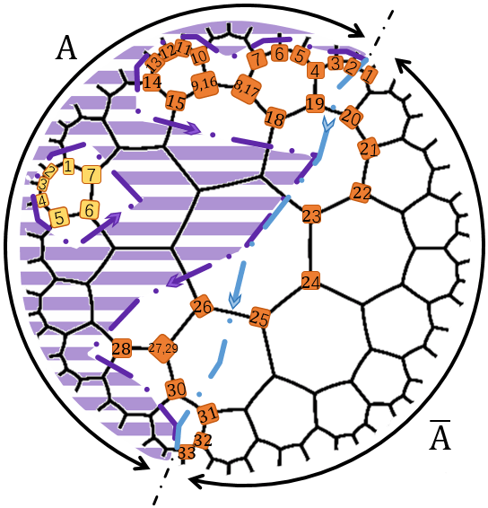
Figure 19: A directed cut $C$ during the course of the greedy algorithm starting from $A$ is marked by purple dot-dashed lines, which consists of two connected components, an open curve and a closed curve. The open curve is denoted by $[N_{1},N_{2},\cdots,N_{33}]$, with $N_{8}=N_{17},\,N_{9}=N_{16}$ and $N_{27}=N_{29}$. The closed curve is denoted by $(N_{1}^{\prime},N_{2}^{\prime},\cdots,N_{7}^{\prime})$. The sub tensor networks $\Phi$ absorbed by the greedy algorithm is shaded with purple strips. A minimal secant geodesic $G_{m}$ is marked by blue dot-dashed line.

A greedy algorithm can start from the interval $\bar{A}$ as well. In Fig.14 14 14 18 18 18, we show the final results of greedy algorithm on several tensor networks with specific intervals $A$ and $\bar{A}$, which are shaded with different colors respectively. In Fig.14 and 18, all the tensor chains are protected under the action of greedy algorithm such that no shaded region presents in those networks.

In above plots one may notice that some CP tensor chains are absorbed by greedy algorithm, which apparently conflicts with the fact that CP tensor chain should be protected. We point out that this phenomenon ascribes to the fact that the endpoints of CP tensor chains belong to the interval $A$ or $\bar{A}$ on the boundary as well. For instance, consider the greedy algorithm starting from $\bar{A}$, as shown in Fig.20. We define $\dot{\bar{A}}$ to be the interval between one endpoint of a CP tensor chain, which is an uncontracted edge on the boundary within $\bar{A}$, and the most neighboring endpoint of $\bar{A}$. Generally, the width of $\dot{\bar{A}}$ is equal to the geodesic distance between the CP curve and its axis, i.e. $d_{c}=\text{arctanh}(\lambda_{c})$. We firstly consider the greedy algorithm starting from a sub-interval $\bar{A}-\dot{\bar{A}}$. At this stage greedy algorithm stops before it touches the CP tensor chain indeed. However, for practice when we calculate the reduced density matrix $\rho_{A}$, the contraction on the endpoints of CP tensor chain, namely uncontracted edges within $\dot{\bar{A}}$, must be taken into account by definition. At this stage the CP tensor chain may fail to be protected under the action of greedy algorithm, as shown in Fig.14. We refer it as the boundary effect of greedy algorithm. Nevertheless, we remark that this boundary effect is weak in the sense that it just absorbs finite layers (most possibly, only one layer) of tensors, and we will elaborate it when we study the ES of tensor networks in Section VII.

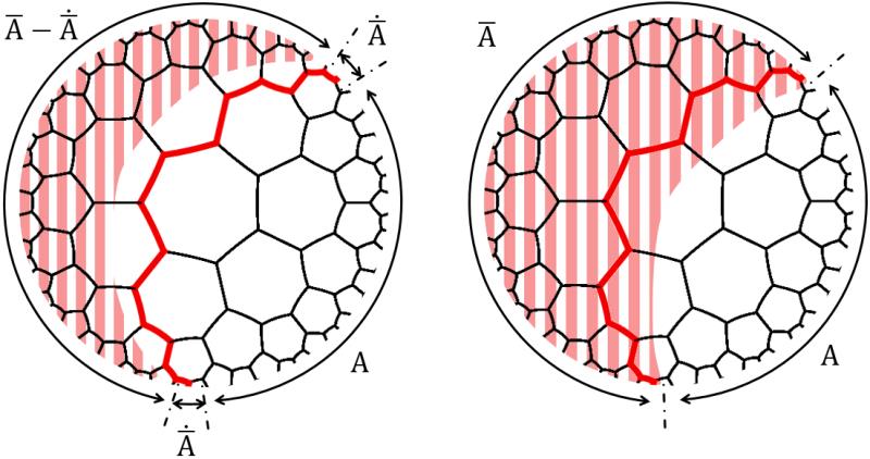
Figure 20: Boundary effect of greedy algorithm in the tensor network with $\left\{7,3\right\}$ tiling and $S_{c}=\left\{\begin{bmatrix}[0.5]1\\ 2\end{bmatrix},\begin{bmatrix}[0.5]1&0&1\\ 1&1&1\end{bmatrix}\right\}$. Interval $\bar{A}$ is split into $\bar{A}-\dot{\bar{A}}$ and $\dot{\bar{A}}$. The CP tensor chain is denoted by the polyline in red.

VI Quantum error correction (QEC)

In this section we will concentrate on how to justify the ability of QEC for a tensor network based on the properties of CP tensor chain.

VI.1 Greedy algorithm and QEC

The whole story of QEC on tensor networks is based on the Hilbert space associated with uncontracted edges which introduce extra degrees of freedom in the bulk and the corresponding code subspace in the Hilbert space on the boundary. The correction to the code subspace after erasing an interval $A$ on the boundary is equivalent to pushing a bulk operator in the wedge of the interval $\bar{A}$ to the interval $\bar{A}$ on the boundary Almheiri:2014lwa . Technically, following Pastawski:2015qua , the procedure of QEC involves in three steps: (1) acting on an uncontracted index in the bulk with an operator; (2) pushing the operator from this index in the bulk to the indexes in the network; (3) pushing it to the boundary further.

In our current work we will ignore the Hilbert space in the bulk since our main purpose is to realize the algorithm of QEC on tensor networks. We will skip step 1 and begin at step 2, by directly inserting an operator into the contracted edges in the interior. In the language of tensor chain, we can insert an operator $O$ between tensor chain $M$ and $M^{\prime}$

$$\sum_{B}M^{A}_{B}M^{\prime B}_{C}\to\sum_{BD}M^{A}_{B}O^{B}_{D}M^{\prime D}_{C}.$$ (67)

No matter which way one adopts to insert an operator into the network, the latter processes of QEC are the same. Thanks to tensor constraint, we can push an operator $O$ through a tensor chain $M\in S_{D}$ and the output operator can be rewritten as $O^{\prime}$, namely

$$\sum_{B}O^{A}_{B}M^{B}_{C}\propto\sum_{B}M^{A}_{B}O^{\prime B}_{C},\quad O^{\prime B}_{C}=\sum_{AD}(M^{B}_{A})^{*}O^{A}_{D}M^{D}_{C}.$$ (68)

Specifically, without uncontracted indexes in the bulk, equation (67) is just the reflection of step 2 above and equation (68) depicts step 3. After all, the terminology ‘QEC’ in this paper refers to the above interpretation.

All above operations can be demonstrated by diagrams. Taking the tensor network with $\left\{7,3\right\}$ tiling as an example. The insertion of an operator is illustrated as

$$\includegraphics[height=40.0pt]{73adding.png}.$$ (69)

While employing tensor constraints (14), the process of pushing an operator through tensor chains can be illustrated as

$$\includegraphics[height=40.0pt]{731pushing1.png},\quad\quad\includegraphics[height=40.0pt]{731pushing2.png}$$ (70)

$$\includegraphics[height=40.0pt]{7311pushing1.png},\quad\quad\includegraphics[height=40.0pt]{7311pushing2.png}.$$ (71)

One can successively push operators through tensor chains in $S_{D}$. Operators may be finally pushed to an interval on the boundary or not, depending on the structure of tilings and tensor constraints. Actually, tensor pushing is the reverse procedure of greedy algorithm, where pushing an operator through tensor chain $M\in S_{D}$ is reverse to the procedure of absorbing a tensor chain $M$ into the shaded region of a tensor network.

Definition 12.

We say that a tensor network enjoys QEC if any operator inserted into the bulk of the network can be pushed to an interval on the boundary.

In Fig.14 and 14, an inserted operator $O$ is successfully pushed to $\bar{A}$. We remark that if the operator is inserted into the region enclosed by the CP tensor chain and interval $\bar{A}$, as illustrated in Fig.14, then it can be pushed to $\bar{A}$. In other word, after erasing an interval $A$, most of those points in the wedge of $\bar{A}$ can be recovered by QEC.

While if the operator is inserted into the region enclosed by the CP tensor chain and the geodesic bounded by $\partial\bar{A}$, the situation becomes subtle and it is not guaranteed that the operator can always be pushed to $\bar{A}$. On one hand, if the inserted operator is close to CP tensor chain, as illustrated in Fig.14, then it may still be pushed to a subinterval in $\bar{A}$. While, now the bound of such subinterval is approaching to $\partial\bar{A}$. In this figure we notice that a lot of arrows, which denote the trajectory of pushing the operator through, go across the geodesic and then radiate out in a wide region, in contrast to the process in Fig.14. Such phenomenon indicates that the information of an operator can only be recovered in a wide range of the boundary, implying the function of QEC in Fig.14 is weaker than that in the tensor network in Fig.14. It may be related to the approximate QEC Schumacher:2002aqe ; Almheiri:2014lwa . On the other hand, if the operator is rather close to the geodesic bounded by $\partial\bar{A}$, it may not be pushed to $\bar{A}$ any more.

VI.2 CP curves and QEC

The geometric description of CP tensor chain in Section IV provides us a way to describe QEC over $H^{2}$ space as well. Given a subsystem $\bar{A}$ on the boundary, one may ask whether an operator acting on point $x$ which locates inside the wedge of $\bar{A}$ can be pushed to $\bar{A}$. For a simply connected interval $\bar{A}$, we denote its two endpoints as $u$ and $v$, respectively. Then these two points together the point $x$ can uniquely determine a hypercircle $H$ in $H^{2}$ space. The sub network in region $\Omega$ enclosed by $H$ and $\bar{A}$ defines a mapping $\Phi$ from the Hilbert space associated with the edges on $H$ to the Hilbert space associated with the edges on $\bar{A}$. If and only if $\Phi$ is proportional to an isometry, then the operator can be pushed to the boundary, thus implementing QEC in an operator scenario. Otherwise the operator can not be pushed into the region specified by $\bar{A}$, and the recovery of such an operator will be prevented by erasing $A$ such that QEC fails.

To check whether $\Phi$ is isometric or not, one needs to evaluate the inner product $\Phi\Phi^{\dagger}$, which is directly determined by the imposed tensor constraints $S_{c}$. During the evaluation process, the most difficult step is to simplify the contraction $MM^{\dagger}$, where $M$ is the boundary tensor chain of $\Phi$ on $H$. So to figure out whether $\Phi$ is isometric or not, our final task is to justify whether $M$ is protected or not under tensor contractions which are subject to $S_{c}$.

Fortunately, our discussion in the section of critical protection has provided an answer to this question. One can justify this by comparing the geodesic curvature $\lambda$ of the hypercircle $H$ with the the curvature of CP curve $\lambda_{c}$. If $\lambda>\lambda_{c}$, then $M$ is unprotected; if $\lambda<\lambda_{c}$, then $M$ is protected.

As a result, given a subsystem $A$ on the boundary, we find a geodesic connecting two end points of the subsystem $A$ and a CP curve between the geodesic and $\bar{A}$. Whether an operator at $x$ can be pushed into $\bar{A}$ depends on the geodesic curvature of the hypercircle passing through $x$. For those points inside the region enclosed by boundary $\bar{A}$ and the CP curve, an operator can be recovered by QEC since the geodesic curvature of hypercircles is greater than $\lambda_{c}$; while for those points inside the region enclosed by the CP curve and the geodesic an operator can not be recovered by QEC since the geodesic curvature is less than $\lambda_{c}$.

When a tiling of $H^{2}$ is specified, $\kappa_{c}$ is inversely related to $\lambda_{c}$. Because $\kappa$ is more easily calculated than $\lambda$, one can alternatively compare the average reduced interior angle $\kappa$ of a hypercircle with the average reduced interior angle of CP tensor chain $\kappa_{c}$. For a given tiling, recall that the tensor chain corresponding to a horocircle with $\lambda_{h}=1$ has average reduced interior angle $\kappa_{h}$ in (59). Moreover, once $S_{c}$ is specified, then $\lambda_{c}$ and $\kappa_{c}$ are determined as well. Whether a tensor network enjoys QEC or not can be justified by comparing the value of $\lambda_{c}$ with $\lambda_{h}$ or $\kappa_{c}$ with $\kappa_{h}$, as described below.

If $\lambda_{c}\geq 1$ or $\kappa_{c}\leq\kappa_{h}$, the CP curve is a circle or a horocircle. The geodesic curvature of all hypercircles must be less than $\lambda_{c}$, so no QEC can be implemented by inserting an operator into any point in the bulk and such a tensor network do not enjoy QEC. For instance, those tensor networks in Fig. 14 and 18 belong to this class. It matches the fact that greedy algorithm does not iterate in these tensor networks.

Similarly, if $\lambda_{c}<1$ or $\kappa_{c}>\kappa_{h}$, the CP curve is a hypercircle. An operator inserted into the region enclosed by the CP tensor chain and $\bar{A}$ can be recovered by QEC and such a tensor network enjoy QEC. For instance, all the other tensor networks except Fig.14 and 18 in this paper belong to this class. Nevertheless, given an interval $\bar{A}$, the region that can be recovered is different for different constraints.

We summarize the above results about the function of QEC in a network in Fig.25.

VII Entanglement spectrum (ES)

Next we focus on the evaluation of entanglement spectrum for a given tensor network, and argue that the flatness of ES can be justified with the power of critical protection in general cases.

VII.1 Reduced density matrix

A tensor network $\Psi$ gives a state $\left|\Psi\right\rangle$ in the Hilbert space defined on its uncontracted edges on the boundary. Given an interval $A$ on the boundary, one can obtain the reduced density matrix of $A$ by tracing out the complementary region $\bar{A}$, namely

$$\rho_{A}=\mathrm{Tr}_{\bar{A}}\left|\Psi\right\rangle\left\langle\Psi\right|.$$ (72)

We are concerned with the issue whether the reduced density matrix $\rho_{A}$ has a flat spectrum, which means that all the non-zero eigenvalues of $\rho_{A}$ are identical. This statement can be alternatively rephrased as the following propositions:

• All the orders of Renyi entropy

  $$S_{A,n}=-\frac{1}{n-1}\ln\frac{\mathrm{Tr}\left(\rho_{A}^{n}\right)}{\left(\mathrm{Tr}\rho_{A}\right)^{n}}$$ (73)

  are identical, namely independent of $n$.

• Reduced density matrix satisfies the relation

  $$\rho_{A}^{2}\propto\rho_{A}.$$ (74)

As indicated at the beginning of this paper, $\rho_{A}$ of the ground state of $CFT_{2}$ satisfies (1) and exhibits a non-flat ES. The gravitational dual result of $AdS_{3}$ vacuum coincides with the above result as well. Now we would like to check whether the ES of a tensor network state is flat or not. For this purpose it is convenient to check the relation in (74) by manipulating tensor networks.

First we disclose the key role of CP tensor chain in identifying the protected region in a tensor network. Recall the boundary effect in greedy algorithm, we intend to separate the procedure of taking trace on $\bar{A}$ into following two steps

$$\rho_{A}=\mathrm{Tr}_{\bar{A}}\left|\Psi\right\rangle\left\langle\Psi\right|=\mathrm{Tr}_{\dot{\bar{A}}}\mathrm{Tr}_{\bar{A}-\dot{\bar{A}}}\left|\Psi\right\rangle\left\langle\Psi\right|.$$ (75)

In the following, we will take tensor networks with $\left\{7,3\right\}$ tiling as examples to demonstrate the evaluation of ES by manipulating tensor networks. The results have previously been collected in Table 1.

VII.1.1 Non-flat ES

First of all, we point out the evaluation of ES depends on the choice of the interval $A$ on the boundary. We will see that, for constraints $S_{c}=\left\{\begin{bmatrix}[0.5]1\\ 2\end{bmatrix},\begin{bmatrix}[0.5]1&0&1\\ 1&1&1\end{bmatrix}\right\}$, the ES of $\rho_{A}$ for any relatively large interval $A$ is non-flat. We call the tensor network generally has a non-flat ES. The word “generally” means that the ES is always non-flat unless fine-tuning tensor $T$ and $E$. Throughout this paper when we say that a tensor network has a non-flat ES, we refer to the above statement.

Firstly, we trace out the degrees of freedom in $\bar{A}-\dot{\bar{A}}$ to obtain the reduced density matrix. During this procedure the structure of tensor network is simplified due to the tensor constraints generated by $S_{c}$, see Fig.21 (a-c). Specifically, those tensors in the wedge of $\bar{A}$ are contracted into identity matrices, which is just the process of the greedy algorithm starting from $\bar{A}-\dot{\bar{A}}$ in the previous section. One can repeatedly consider this process until it reaches a final stage that the network can not be simplified any more, as shown in Fig.21(c). The terminal boundary forms a polyline in red as marked in Fig.21. As a matter of fact, such a polyline is nothing but a CP tensor chain as we have defined in previous section. From this figure we perceive that, before the trace of uncontracted edges in $\dot{\bar{A}}$ is taken into account, the operation induced by the greedy algorithm can not enter the region enclosed by CP tensor chain and $A$, which is exactly the reason why we call it critically protected tensor chain.

Now the next step is to evaluate $\mathrm{Tr}_{\dot{\bar{A}}}$, namely tracing the degrees of freedom associated with uncontracted edges on the boundary which are mostly neighboring to $A$. The process is illustrated in Fig.21(d)(e). We notice that the network structure can be further simplified such that CP tensor chains are absorbed into the shaded region at this step, which is the boundary effect of greedy algorithm as we described in previous section.

The boundary effect of greedy algorithm results from the discretization of $H^{2}$ space, which may not appear in a continuous geometry. In the context of tensor networks, however, according to (75) the uncontracted edges in $\dot{\bar{A}}$ should be contracted. Sometime the contribution of this effect to reduced density matrix becomes subtle, and we should cautiously handle this effect. In other words, whether the ES is flat or not can only be justified after the boundary effect is taken into account.

Now with the reduced density matrix $\rho_{A}$ at hand, we can compute $\rho_{A}^{2}$ by further contracting those uncontracted edges in $A$. One can simplify $\rho_{A}^{2}$ by virtue of tensor constraints, which is parallel to the above process on $\bar{A}$. Boundary effect of greedy algorithm appears as well. Before the boundary effect is taken into account, the greedy algorithm stops at a CP tensor chain, which is the reflection of the CP tensor chain appearing in the contraction on $\bar{A}$ about the geodesic bounded by $\partial A$. Thus, the simplification of $\rho_{A}^{2}$ is equivalent to applying the greedy algorithm to $A$ and $\bar{A}$ successively, as shown in Fig.14.

The calculation of $\rho_{A}^{2}$ is demonstrated in Fig.22. Obviously from this diagram we find that $\rho_{A}^{2}$ can not be simplified to be proportional to $\rho_{A}$ such that equation (74) is not satisfied. Equivalently, from Fig.14, we notice that some tensors are not absorbed by the greedy algorithm starting from $A$ and $\bar{A}$, thus (74) is not satisfied.

Given the above constraints, we point out that as long as $A$ is large enough, $\rho_{A}$ always gives rise to a non-flat ES, independent of the choice of $A$. This assertion will be proved in Subsection VII.3. Right now we just conclude that such a tensor network has a non-flat ES, in agreement with what is found by explicitly computing the eigenvalues of the reduced density matrix in Evenbly:2017htn .

We remark that for the above constraints the corresponding CP curve is a hypercircle. When the CP curve is a horocircle, it approaches the boundary with single intersecting point. Or when the CP curve is a circle, it does not reach the boundary. For both cases one need not consider the boundary effect separately, and the ES is usually non-flat for CP circles since the region enclosed by the circle is protected.

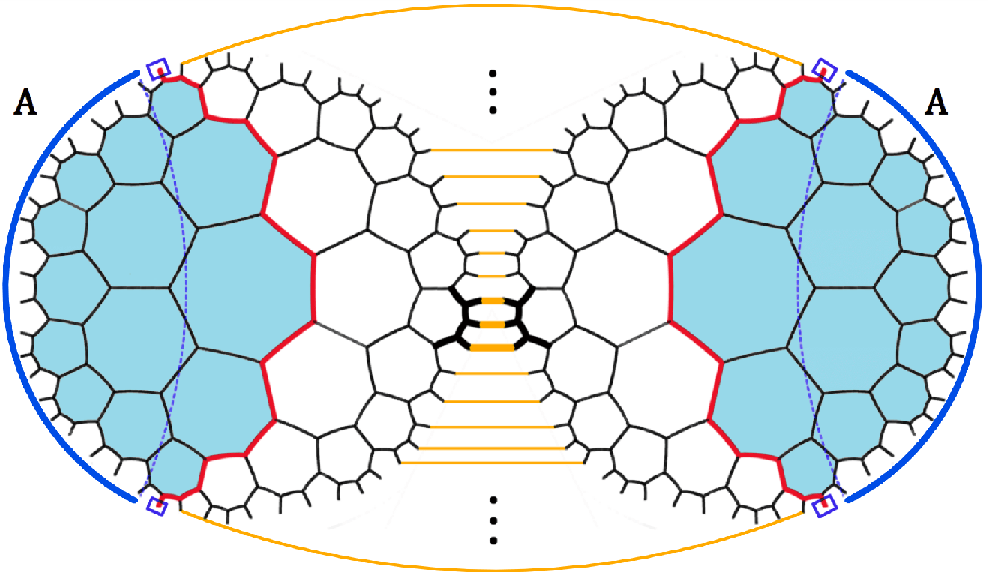
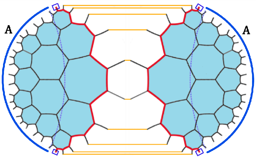
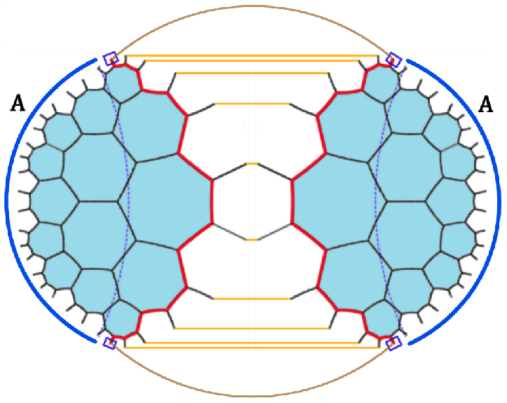
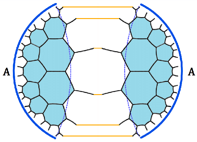
Figure 21: The evaluation of $\rho_{A}$. The interval $A$ is marked by solid lines in blue. The geodesic bounded by $\partial A$ is plotted as a dashed line in blue. The CP tensor chain is marked by a solid line in red, and its two endpoints on the boundary are marked by two blue rectangles. (a) The contractions of indexes in $\bar{A}$ are illustrated by orange lines. (b) Before the endpoints of CP tensor chain are contracted, CP tensor chains are not absorbed. (c) The contractions of the endpoints of CP tensor chain on the boundary is marked by brown lines. (d) CP tensor chains are absorbed at the final stage.

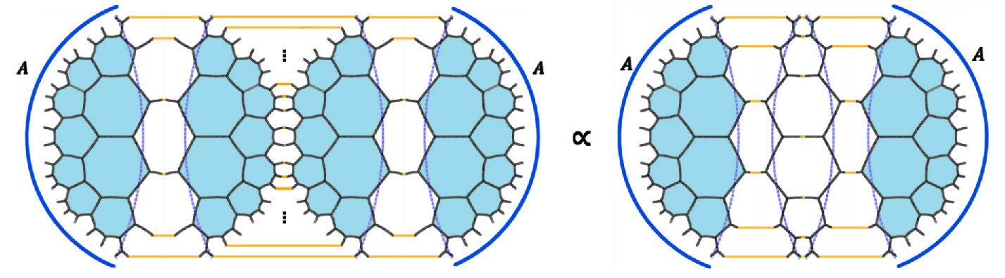
Figure 22: The diagram for the evaluation of $\rho_{A}^{2}$. (74) is not satisfied.

VII.1.2 Flat ES

We have pointed out that one equivalent way to check the relation in (74) is to consider the greedy algorithm starting from $A$ and from $\bar{A}$ successively. Let us take Fig.14 as an example, where $S_{c}=\left\{\begin{bmatrix}[0.5]1\\ 2\end{bmatrix},\begin{bmatrix}[0.5]1&1\\ 1&1\end{bmatrix}\right\}$. We observe that the union of these two shaded regions covers the whole tensor network, implying that all the tensors are absorbed by the greedy algorithm. Therefore, (74) is satisfied and ES has to be flat. We call the tensor network has a flat ES.

VII.1.3 Mixed ES

From Fig.14, we know that, for $S_{c}=\left\{\begin{bmatrix}[0.5]1\\ 2\end{bmatrix},\begin{bmatrix}[0.5]1&0&1&0&1\\ 1&1&0&1&1\\ \end{bmatrix}\right\}$, the ES of $\rho_{A}$ can be flat or non-flat, depending on the choice of $A$. We call the tensor network has a mixed ES.

VII.2 Geometric point of view on ES

In the tensor network realization of AdS/CFT, a tensor network is usually treated as the wavefunction $\Psi$ of the ground state. Alternatively, when an interval $A$ on the boundary is given, we notice that $\Psi$ can be understood as a mapping from the Hilbert space on $A$ to the Hilbert space on $\bar{A}$. So $\Psi$ can be regarded as a matrix $\Psi^{A}_{\bar{A}}$, where two indexes $A$ and $\bar{A}$ represent the degrees of freedom on two subsystems $A$ and $\bar{A}$, respectively.

The notion of critical protection provides us an efficient way to visualize the simplification of tensor networks under the tensor contractions which are subject to tensor constraints. To make this process more transparent, we firstly intend to decompose a network into some sub networks. As seen in previous subsections, when the indexes on $A$ or $\bar{A}$ are contracted, the greedy algorithm will stop at some nodes. Let us firstly neglect the boundary effect, then the skeletons of connecting those nodes will form two CP tensor chains, which are neighboring to the geodesic bounded by $\partial A$.

First of all, we point out that when $\lambda_{c}\geq 1$ or $\kappa_{c}\leq\kappa_{h}$, all the hypercircles are protected since their geodesic curvatures are less than $\lambda_{c}$. So a non-flat ES is guaranteed. In the following, we will focus on the non-trivial case, $\lambda_{c}<1$ or $\kappa_{c}>\kappa_{h}$, where CP curves are hypercircles.

We denote the CP curve close to $A$ or $\bar{A}$ as $H_{A}$ or $H_{\bar{A}}$, respectively. The region enclosed by two CP curves is called CP region $\Omega_{c}$. Those tensors in the CP region form a sub tensor network $\Psi_{c}$, which is a mapping from $H_{A}$ to $H_{\bar{A}}$ and is denoted as $(\Psi_{c}){}^{H_{A}}_{H_{\bar{A}}}$. Similarly, $H_{A}$ and $A$ enclose a sub tensor network $\Phi_{A}$, which defines a mapping $(\Phi_{A}){}^{A}_{H_{A}}$; $H_{\bar{A}}$ and $\bar{A}$ enclose a sub tensor network $\Phi_{\bar{A}}$, which defines a mapping $(\Phi_{\bar{A}}){}^{\bar{A}}_{H_{\bar{A}}}$. Since the tensors outside $H_{A}$ are not protected under the contraction of $A$, the mapping $(\Phi_{A}){}^{A}_{H_{A}}$ from $H_{A}$ to $A$ should be proportional to an isometry. Similarly, the mapping $(\Phi_{\bar{A}}){}^{\bar{A}}_{H_{\bar{A}}}$ from $H_{\bar{A}}$ to $\bar{A}$ is proportional to an isometry as well. It is denoted as

$$\Phi_{A}^{\dagger}\Phi_{A}\propto I,\quad\Phi_{\bar{A}}^{\dagger}\Phi_{\bar{A}}\propto I^{\prime},$$ (76)

where the indexes are abbreviated and $I$ ($I^{\prime}$) is identity matrix on $A$ ($\bar{A}$).

Finally, the full matrix $\Psi^{A}_{\bar{A}}$ can be represented as the product of matrices

$$\Psi=\Phi_{A}\Psi_{c}\Phi_{\bar{A}}^{\dagger}.$$ (77)

Then it is easy to see

$$\rho_{A} = \Psi\Psi^{\dagger}=\Phi_{A}\Psi_{c}\Phi_{\bar{A}}^{\dagger}\Phi_{\bar{A}}\Psi_{c}^{\dagger}\Phi_{A}^{\dagger}\propto\Phi_{A}\Psi_{c}\Psi_{c}^{\dagger}\Phi_{A}^{\dagger},$$ (78)

$$\rho_{A}^{2} = \Psi\Psi^{\dagger}\Psi\Psi^{\dagger}\propto\Phi_{A}\Psi_{c}\Psi_{c}^{\dagger}\Psi_{c}\Psi_{c}^{\dagger}\Phi_{A}^{\dagger},$$ (79)

where (76) is used. A flat ES in (74) means that

$$\Psi_{c}\Psi_{c}^{\dagger}\Psi_{c}\Psi_{c}^{\dagger}\propto\Psi_{c}\Psi_{c}^{\dagger}.$$ (80)

We present a schematic diagram to demonstrate the decomposition of tensor network state as well as the calculation of $\rho_{A}$ and $\rho_{A}^{2}$ in Fig.LABEL:FigrhoA2. The condition for flat ES (80) is illustrated in Fig.24. This figure reveals that whether the ES is flat or not depends on the thickness of the CP region where the thickness of the CP region is defined by the distance between the two CP curves.

Equivalently, from above derivation we notice that the flatness of ES may be checked by observing the result of the greedy algorithm starting from $A$ and from $\bar{A}$ successively, which figures out the region of isometry between tensor chains in (76). If all the tensors are absorbed by the greedy algorithm, then (80) is valid and the ES is flat, and vice versa.

Once the boundary effect is considered, as we showed in previous section, CP tensor chains on the boundary of the CP region $\Omega_{c}$ are not protected any more under the greedy algorithm. Nevertheless, only a finite thickness of the CP region will be absorbed. In Fig.22, since those tensors close to the geodesic are not absorbed, the tensor network has a non-flat ES.

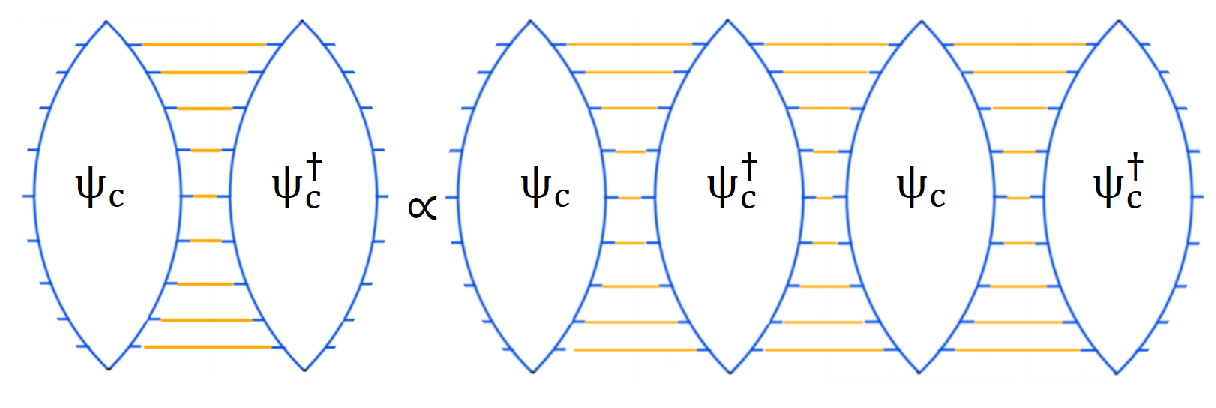
Figure 24: The condition of flat ES.

The experience one has gained from this picture is that the thickness of CP region determines whether the ES is flat or not. Without the boundary effect, the boundary of CP region is composed of two CP curves, so its thickness is $2d_{c}$, where $d_{c}=\text{arctanh}(\lambda_{c})$ is the geodesic distance between the CP curve (hypercircle) and its axis. Due to the boundary effect, the CP tensor chain will not be protected any more and the outer layer of the original CP region will be absorbed by greedy algorithm. The thickness of such layers is proximately given by $P$, which is the length of an edge (4). So the thickness of CP region decrease to $2d_{c}-P$. Since $\Psi_{c}$ is protected, (80) is true only if the thickness of the CP region vanishes.

The evaluation of the geodesic curvature $\lambda$ in a general tensor network is difficult, which prevents us from justifying the flatness of ES with CP curvature $\lambda_{c}$. Alternatively, this job can be done by calculating CP reduced interior angle $\kappa_{c}$, as described in the next subsection.

VII.3 The reduced interior angle of CP tensor chain and ES

In previous subsections we have shown the relation between the flatness of ES and the structure of CP tensor chains under the action of greedy algorithm. In this subsection we show that the flatness of ES can be justified based on the value of $\kappa_{c}$. Specifically, we find that the bigger is $\kappa_{c}$, the stronger is the ability of QEC while ES more easily becomes flat, as shown in Fig.25. In this figure we further introduce three quantities which are determined by the $\{b,a\}$ tiling:

$$\kappa_{h}=\frac{a}{2}-\frac{a-2}{2}\sqrt{\frac{ab-2a-2b}{ab-2a-2b+4}},\quad\kappa_{1}=\frac{b}{b-2},\quad\kappa_{0}=\frac{a}{2}.$$ (81)

Because of (3), the relation $\kappa_{h}<\kappa_{1}<\kappa_{0}$ always holds. If $\kappa_{c}\in(1,\kappa_{h})$, it turns out the network is not able to implement QEC but has non-flat ES, as indicated in Fig.14 and 18. If $\kappa_{c}\in(\kappa_{h},\kappa_{1})$, then the network can implement QEC and has non-flat ES, as shown in Fig.14 and 18. If $\kappa_{c}\in[\kappa_{1},\kappa_{0})$, the ability of QEC will become stronger but the ES will become “mixed” , as shown in Fig.14 and 18. Finally, if $\kappa_{c}=\kappa_{0}$, the quality of QEC becomes better but the ES has to be flat, which is exactly the property of perfect tensors, as shown in Fig.14 and 18.

Correspondingly, we may propose a geometric quantity in $H^{2}$ space which plays a similar role as $\kappa_{c}$ in tensor network. This quantity is the geodesic curvature $\lambda_{c}$ of CP curve. Given a tiling, $\lambda_{c}$ can be calculated by using $\kappa_{c}$. A schematic relation between $\lambda_{c}$ and QEC and ES is also illustrated in Fig.25. While, we do not have general expressions for the bounds $\lambda_{0}$ and $\lambda_{1}$ so far, which corresponds to $\kappa_{0}$ and $\kappa_{1}$, respectively.

Until now, we have constructed a general framework for tensor networks with tensor constraints, and developed a generalized greedy algorithm to describe the property of critical protection. In the remainder of this paper, we will provide detailed proofs for the quantitative relation between CP tensor chain and QEC as well as ES, and finally complete the classification of tensor networks as illustrated in Fig.25.

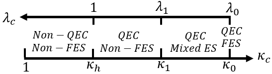
Figure 25: $\lambda_{c}$ and $\kappa_{c}$ can be used to classify the property of QEC and ES in tensor network.

Those statements can be rephrased into following propositions:

• If $\kappa_{c}=\frac{a}{2}$, then $\rho_{A}$ has flat ES for any choice of $A$;

• If $\kappa_{c}<\frac{a}{2}$, then $\rho_{A}$ may have non-flat ES for some choices of $A$;

• If $\kappa_{c}\geq\frac{b}{b-2}$, then $\rho_{A}$ may have flat ES for some choices of $A$;

• If $\kappa_{c}<\frac{b}{b-2}$, then $\rho_{A}$ has non-flat ES for any choice of large $A$.

Now we intend to prove these propositions separately.

VII.3.1 $\kappa_{c}=\frac{a}{2}\Rightarrow$ flat ES

Based on the discussion in Subsection V.2, we will prove the flatness of ES by showing that any directed cut appearing in the process of greedy algorithm is unprotected such that the greedy algorithm will not stop until all the tensors are absorbed.

To prove a directed cut in the process of greedy algorithm is unprotected, one need to find out an unprotected tensor chain connected to the cut. Recall that those directed cuts in greedy algorithm may have many disconnected components. We firstly prove a lemma for a cut containing the structure of twigs or loops, which will greatly simplify the rest of proofs.

Lemma 1.

Given a tensor network with $\left\{b,a\right\}$ tiling and $\kappa_{c}\geq\frac{b}{b-2}$, if a directed cut $C$ contains a connected component whose corresponding sequence of nodes has a form as $[\cdots,N_{0},N_{1},\cdots,N_{k},\cdots]$ with $N_{0}=N_{k}$, or $(\cdots,N_{0},N_{1},\cdots,N_{k},\cdots)$ with $N_{0}=N_{k}$, or $(N_{1},N_{2},\cdots,N_{k})$, then the cut $C$ is unprotected.

Proof.

Denote the sequence of nodes $[N_{1},\cdots,N_{k}]$ as $L_{N}$. We assume that all these nodes in $L_{N}$ are distinct, otherwise we just replace $N_{1}$ and $N_{k}$ by any two nodes which are identical and the following proof is still valid.

When $k=1$, it is only possible that the connected component is a single node $N_{1}$, then the tensor chain $\begin{bmatrix}[0.5]0\\ a\end{bmatrix}$ on $N_{1}$ is connected to $C$. Since $\begin{bmatrix}[0.5]0\\ a\end{bmatrix}\in S_{D}$, $C$ is unprotected.

When $k=2$, the shape of $L_{N}$ is a twig and $N_{1}$ is the endpoint of the twig. Step tensor chain $\begin{bmatrix}[0.5]1\\ a-1\end{bmatrix}$ on $N_{1}$ is connected to $C$, so $C$ is unprotected. For instance, in Fig.19, $N_{27}=N_{29}$ and the sequence $L_{N}=[N_{28},N_{29}]$ forms a twig, $N_{28}$ is the endpoint and $M_{s}$ at $N_{28}$ is connected to the cut.

When $k\geq 3$, those edges between $N_{i}$ and $N_{i+1}$, and the edge between $N_{1}$ and $N_{k}$ in $L_{N}$ form a closed polyline, e.g., see the sequence $[N_{10},N_{11},\cdots,N_{16}]$ in Fig.19. We define the region enclosed by the polyline as $Y$, which consists of $F$ elementary polygons, $E$ edges and $V$ nodes (vertices) which satisfy Euler’s formula

$$F-E+V=1.$$ (82)

Let the reduced interior angle of $Y$ at $N_{i}$ be $x_{i}$ for $i\in\left\{1,2,\cdots,k\right\}$. We have

$$\sum_{i=1}^{k}x_{i}+k+a(V-k)=2E,$$ (83)

$$k\leq V,$$ (84)

$$bF=2E-k.$$ (85)

From above four formulas, we have

$$\sum_{i=1}^{k}x_{i}\leq\frac{b}{b-2}(k-2).$$ (86)

Because $x_{k}\geq 1$, we further have

$$\sum_{i=1}^{k-1}x_{i}\leq\frac{b}{b-2}(k-2)-1.$$ (87)

Those nodes $[N_{1},N_{2},\cdots,N_{k-1}]$ form a tensor chain $M=\begin{bmatrix}[0.5]*&*&\cdots&*\\ n_{1}&n_{2}&\cdots&n_{k-1}\end{bmatrix}$ connected to $C$, where $n_{i}=a-1-x_{i}$ for $i\in\left\{1,2,\cdots,k-1\right\}$. Recall that $\kappa_{c}\geq\frac{b}{b-2}$. Finally,

$$\sum_{i=1}^{k-1}(a-1-n_{i})\leq\kappa_{c}(k-2)-1<\kappa_{c}(k-1)-1.$$ (88)

From Theorem 9, $M$ is unprotected and thus $C$ is unprotected.

In conclusion, when $\kappa_{c}\geq\frac{b}{b-2}$, any cut $C$ containing twigs or loops must be unprotected. ∎

Obviously, $\kappa_{c}=\frac{a}{2}>\frac{b}{b-2}$. Lemma 1 is applicable to this case and those branches forming twigs or loops in a cut will be absorbed by the greedy algorithm. Taking the cut in Fig.19 as an example, we claim that those nodes in $\left\{N_{8},N_{9},\cdots,N_{17}\right\},\left\{N_{27},N_{28},N_{29}\right\}$, and $\left\{N_{1}^{\prime},N_{2}^{\prime},\cdots,N_{7}^{\prime}\right\}$ will be absorbed.

As a result, now we can focus on the case that the cut $C$ is single connected and bounded by $\partial A$, which is denoted as $C=[N_{1},N_{2},\cdots,N_{l}]$. Furthermore, these nodes in $C$ are distinct.

With any choice of single interval $A$ on the boundary of a tensor network $\Psi$, we apply the greedy algorithm starting from $A$ and from $\bar{A}$ simultaneously. So two cuts, $C_{A}$ and $C_{\bar{A}}$, appear in $\Psi$ at the same time. We will prove with mathematical induction that when $\kappa_{c}=\frac{a}{2}$, either of these two cuts is unprotected until all the tensors are absorbed.

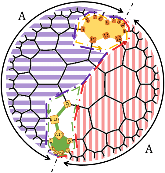
Figure 26: The “directed sum” of two directed cuts $C_{A}$ (purple) and $C_{\bar{A}}$ (red) consists of two directed closed curves $C_{I}$ (green) and $C_{I}^{\prime}$ (yellow). The region $I$ corresponding to $C_{I}$ is filled in green.

Now we consider the configuration of $C_{A}$ and $C_{\bar{A}}$. Both of them are connected to $\partial A$. Besides, they may overlap at some place, where their directions are opposite, as illustrated in Fig.26. Then, we define the “directed sum” of $C_{A}$ and $C_{\bar{A}}$ as the union of them but excluding their overlapped parts. The directed sum consists of one or more closed curves, as shown in Fig.26. Select one of them and denote it as $C_{I}$, which is a directed cut as well. Set the sequence of nodes corresponding to $C_{I}$ to be $(N_{1},N_{2},\cdots,N_{k})$. We connect these nodes $(N_{1},N_{2},\cdots,N_{k})$ with edges in order and enclose a region $I$, which is a union of elementary polygons and edges. At node $N_{i}$, let the reduced outer angles of $I$ be $y_{i}$ and let the number of edges cut by $C_{I}$ be $n_{i}$. Obviously, $y_{i}=n_{i}+1$. Gauss-Bonnet theorem tells that

$$\sum_{i=1}^{k}(\frac{2\pi}{a}y_{i}-\pi)-2\pi=\text{Area}(H)\geq 0,$$ (89)

then

$$\sum_{i=1}^{k}n_{i}\geq\frac{a-2}{2}k+a.$$ (90)

Obviously, those edges cut by $C$ are divided into two parts, one part is cut by $C_{A}$ and the other is cut by $C_{\bar{A}}$. Without loss of generality, we suppose that $C_{A}$ runs from $N_{1}$ to $N_{u+1}$. Moreover, $l_{1}$ edges of $N_{1}$ are cut by $C_{A}$ and $\bar{l}_{k+1}$ edges cut by $C_{\bar{A}}$. While for $N_{u+1}$, $l_{u+1}$ edges are cut by $C_{A}$ and $\bar{l}_{u+1}$ edges are cut by $C_{\bar{A}}$. Obviously, $l_{1}+\bar{l}_{k+1}=n_{1}$ and $l_{u+1}+\bar{l}_{u+1}=n_{u+1}$. We further define that $l_{i}=n_{i}$ for $i=2,3,\cdots,u$ and $\bar{l}_{i}=n_{i}$ for $i=u+2,u+3,\cdots,k$. Then we know that tensor chain $M_{A}=\begin{bmatrix}[0.5]*&*&\cdots&*\\ l_{1}&l_{2}&\cdots&l_{u+1}\end{bmatrix}$ is connected to $C_{A}$ and tensor chain $M_{\bar{A}}=\begin{bmatrix}[0.5]*&*&\cdots&*\\ \bar{l}_{u+1}&\bar{l}_{u+2}&\cdots&\bar{l}_{k}\end{bmatrix}$ is connected to $C_{\bar{A}}$. From (90),

$$\sum_{i=1}^{u+1}l_{i}+\sum_{i=u+1}^{k+1}\bar{l}_{i}=\sum_{i=1}^{k}n_{i}\geq\frac{a-2}{2}k+a=(u+1)\frac{a-2}{2}+1+(k-u+1)\frac{a-2}{2}+1.$$ (91)

So,

$$\sum_{i=1}^{u+1}l_{i}\geq(u+1)\frac{a-2}{2}+1\quad\text{or}\quad\sum_{i=u+1}^{k+1}\bar{l}_{i}\geq(k-u+1)\frac{a-2}{2}+1,$$ (92)

i.e.

$$\sum_{i=1}^{u+1}(a-1-l_{i})\leq(u+1)\kappa_{c}-1\quad\text{or}\quad\sum_{i=u+1}^{k+1}(a-1-\bar{l}_{i})\leq(k-u+1)\kappa_{c}-1.$$ (93)

From Theorem 9, either of $M_{A}$ or $M_{\bar{A}}$ is unprotected, so either of $C_{A}$ or $C_{\bar{A}}$ is unprotected. Thus the greedy algorithm will keep going on until $\text{Area}(H)=0$ at least, which means two cuts $C_{A}$ and $C_{\bar{A}}$ are overlapped such that all tensors are absorbed. Then the ES is flat.

VII.3.2 $\kappa_{c}<\frac{a}{2}\Rightarrow\exists$ non-flat ES

Next we intend to prove when $\kappa_{c}<\frac{a}{2}$, there exists non-flat ES for some choices of single interval $A$ on the boundary.

Thanks to Theorem 9, when $a$ is odd, we can specifically choose $A$ on the boundary such that the structure as shown in Fig.27 is protected under the action of the greedy algorithm starting from either side. A tensor network with a special choice for $A$ is shown in Fig.27, where the structures enclosed by dashed red circles are protected and prevent the ES from being flat.

When $a$ is even, similarly one can choose $A$ appropriately such that the structure as shown in Fig.27 is protected. Then the ES is non-flat.

We remark that such kind of protected structures is common in tensor networks, especially when the network is large enough. So we intend to argue that when $\kappa_{c}<\frac{a}{2}$, most choices of interval $A$ will lead to non-flat ES.

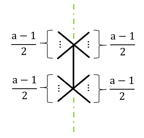
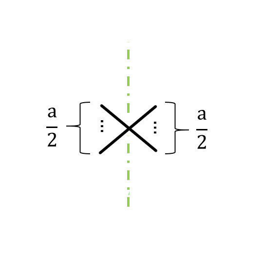
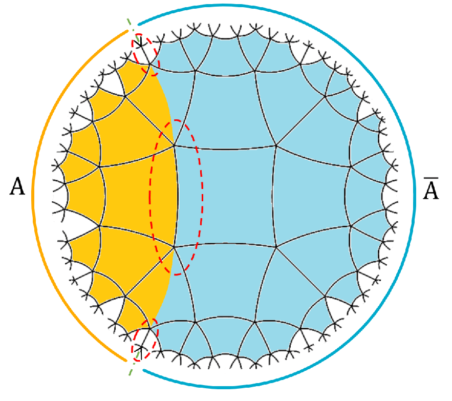
Figure 27: The green dashed lines in (a) and (b) are boundaries which divide edges of the tensors into two parts; The green dashed lines in (c) are the boundaries which divide the tensor network into two parts. In (c) $\frac{a-1}{2}=2$ and the structure in the red circle cannot be contracted

VII.3.3 $\kappa_{c}\geq\frac{b}{b-2}\Rightarrow\exists$ flat ES

In previous subsection we have learned that when $\kappa_{c}<\frac{a}{2}$, ES being non-flat is a common phenomenon. Nevertheless, we point out that when $\kappa_{c}\geq\frac{b}{b-2}$, it is possible to construct single interval whose ES is flat.

Next we just prove the existence of flat ES by constructing a specific interval $A$ with “minimal secant geodesic”, which is obtained by following steps (Fig.19). We start from the midpoint of an edge between two uncontracted edges on the boundary, then connect this point with the midpoint of another edge in the polygon which has the farthest distance to this point. Next we choose the neighboring polygon of this new midpoint in the bulk and connect the midpoint with the other farthest midpoint in this polygon. Repeat above steps until it reaches the boundary of the network. The trajectory forms a geodesic called minimal secant geodesic, denoted by $G_{m}$. It should be noticed that for a polygon with odd edges, there are two middle points which are the farthest from the specified midpoint, one to the left and the other to the right, as shown in Fig.28. We need choose these two midpoints by turn in above steps, as shown in Fig.19.

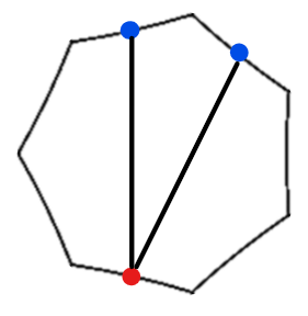
Figure 28: In $b=7$, so for a given red midpoint there are two blue midpoints which are the farthest.

A minimal secant geodesic $G_{m}$ divides the boundary of network into two parts $A$ and $\bar{A}$, which almost have the same size.

We will show that for such a division, the corresponding ES is flat by proving that the greedy algorithm starting from either $A$ or $\bar{A}$ does not stop until the sequence of cuts reaches $G_{m}$. The proofs for $A$ and $\bar{A}$ are parallel. So we only prove the case for $A$.

Similarly, thanks to Lemma 1, we focus on the case that the cut $C$ is single connected and connected to $\partial A$, which is denoted as $C=[N_{1},N_{2},\cdots,N_{l}]$, with distinct nodes.

We give $G_{m}$ a direction such that $\Phi$ is on its right hand side. Then $G_{m}$ becomes a directed cut which is denoted as $[N_{1}^{\prime},N_{2}^{\prime},\cdots,N_{m}^{\prime}]$. By definition, these nodes are distinct.

When $C$ and $G_{m}$ are not overlapped, the edges connecting those nodes in $C$ and $G_{m}$ at least form a polygon. In general, they may enclose one or more polygons, as illustrated in Fig.19.

We pick out any one of them and label it as $Y$. Let the set of those nodes on the boundary of $Y$ to be the union of $[N_{p+1},N_{p+2},\cdots,N_{p+u}]$ in $C$ and $[N_{q+1}^{\prime},N_{q+2}^{\prime},\cdots,N_{q+v}^{\prime}]$ in $G_{m}$. $N_{p+1}$ and $N_{q+1}^{\prime}$ are neighboring to each other. $N_{p+u}$ and $N_{q+v}^{\prime}$ are neighboring to each other. We naturally have $u\geq 2$ after excluding the cases in Lemma 1. Let the reduced interior angle of $Y$ at $N_{p+i}$ as $x_{i}$ for $i\in\left\{1,2,\cdots,u\right\}$ and the reduced interior angle of $Y$ at $N_{q+j}$ as $x_{j}^{\prime}$ for $j\in\left\{1,2,\cdots,v\right\}$. Similar to the relation in (86) in the proof of Lemma 1, for $Y$, we have

$$\sum_{i=1}^{u}x_{i}+\sum_{j=1}^{v}x_{j}^{\prime}\leq\frac{b}{b-2}(u+v-2).$$ (94)

Suppose that the part $[N_{q+1}^{\prime},N_{q+2}^{\prime},\cdots,N_{q+v}^{\prime}]$ crosses $w$ elementary polygons. Due to the special construction of $G_{m}$, we have the relation

$$v<\frac{w}{2}(b-2)+2.$$ (95)

So, we have

$$\sum_{j=1}^{v}x_{j}^{\prime}=v+w-1>\frac{b}{b-2}(v-2)+1.$$ (96)

Plugging it into (94), we obtain

$$\sum_{i=1}^{u}x_{i}<\frac{b}{b-2}u-1\leq\kappa_{c}u-1.$$ (97)

On $[N_{p+1},N_{p+2},\cdots,N_{p+u}]$, tensor chain $M=\begin{bmatrix}[0.5]*&*&\cdots&*\\ n_{1}&n_{2}&\cdots&n_{u}\end{bmatrix}$ is connected to $C$, where $n_{i}=a-1-x_{i}$ for $i\in\left\{1,2,\cdots,u\right\}$. From (97) and Theorem 9, we know $M$ is unprotected, thus $C$ is unprotected.

In conclusion, once $C\neq G_{m}$, $C$ is unprotected and the greedy algorithm progresses. So those tensors between $A$ and $G_{m}$ will be absorbed. In parallel, those tensors between $\bar{A}$ and $G_{m}$ will be absorbed under the greedy algorithm starting from $\bar{A}$. Finally, the sequence of cuts reaches $G_{m}$, leading to a flat ES.

VII.3.4 $\kappa_{c}<\frac{b}{b-2}\Rightarrow$ non-flat ES

Here we prove that when $\kappa_{c}<\frac{b}{b-2}$, the ES of a single and large interval $A$ is non-flat. Perhaps this argument is the most important part in this section because it supplies us a quantitative criteria to justify if a tensor network has a not-flat ES.

Consider a single interval $A$ and its complement $\bar{A}$ on the boundary of a given tensor network. There exists a continuous line, called $G$, connecting two ending points of $A$ with a minimal cuttings on the edges of the network. The line $G$ divides the whole network into two sub tensor networks (see Fig.29).

It is noticed that the nearest neighboring tensors of line $G$ form two tensor chains. We call these two tensor chains as $M_{A}$ and $M_{\bar{A}}$, respectively. As an example, the skeletons of these two tensor chains are marked in Fig.29. We set all the indexes associated with the edges cut by line $G$ as upper indexes, while the other indexes are lower indexes.

Assume that $M_{A}$ has $k_{A}$ nodes, and $M_{\bar{A}}$ has $k_{\bar{A}}$ nodes. Set the number of elementary polygons crossed by line $G$ to be $F$. Then we have two equations

$$\begin{split}&\kappa(M_{A})k_{A}+\kappa(M_{\bar{A}})k_{\bar{A}}=bF,\\ &k_{A}+k_{\bar{A}}=(b-2)F+2.\end{split}$$ (98)

Now we provide a proof by contradiction. We assume that the ES would be flat, then $M_{A},M_{\bar{A}}\in S_{D}$. According to Theorem 7, we have

$$\kappa(M_{A})\leq\kappa_{c},\quad\kappa(M_{\bar{A}})\leq\kappa_{c}.$$ (99)

We substitute (99) into (98) and get an inequality as

$$\kappa_{c}\geq\frac{bF}{(b-2)F+2}.$$ (100)

To simulate real AdS spacetime, the number of layers in a network is expected to be large enough. Then for large interval $A$, $F\gg 1$. Since $\frac{2\kappa_{c}}{b-(b-2)\kappa_{c}}$ is a finite number,

$$F>\frac{2\kappa_{c}}{b-(b-2)\kappa_{c}}.$$ (101)

From (100) and (101), we have $\kappa_{c}\geq\frac{b}{b-2}$, contradictory to the initial assumption. Thus, when $\kappa_{c}<\frac{b}{b-2}$, the ES of a single interval $A$ must be non-flat in a network with large layers.

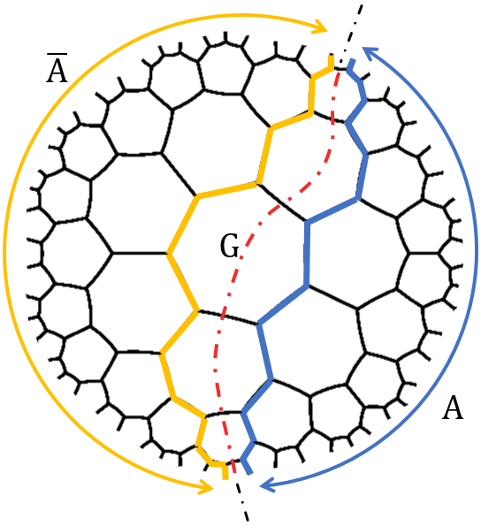
Figure 29: The blue (orange) line is interval $A$ ($\bar{A}$). The red dashed line is line $G$ with minimal cuttings. The blue (orange) polyline corresponds to tensor chain $M_{A}$ ($M_{\bar{A}}$).

VIII Conclusions and outlooks

In this paper we have presented a general framework for tensor networks with tensor constraints based on the tiling of $H^{2}$ space. A notion of critical protection based on the tensor chain has been proposed to describe the behavior of tensor networks under the action of greedy algorithm. In particular, a criteria has been developed with the help of the average reduced interior angle of CP chain such that for a given tensor network the ability of QEC and the flatness of ES can be justified in a quantitative manner. We have also demonstrated a lot of examples of tensor network and discussed their properties of QEC and ES. In general, once the ability of QEC of a tensor network becomes stronger, then its ES becomes flat more easily, and vice versa. By contrast, it is fascinating to notice that AdS spacetime is endowed with these two holographic features with perfect balance indeed. Currently it is still challenging to construct tensor networks which could capture all the holographic features of AdS spacetime. What we have found in this paper may shed light on this issue. Firstly, we have learned that the notion of critical protection provides a description on the limit of information transmission with full fidelity. In the case that the CP curve $H_{c}$ is a circle, i.e. $\lambda_{c}L^{2}>1$, the information in the interior of $H_{c}$ can be transmitted to its surface without loss, where we have restored the AdS radius $L$. While, for a circle $H$ which is larger than $H_{c}$, its interior information can not be transmitted to its surface without loss. So we can say that $H_{c}$ is the maximal boundary which can holographically store the interior information Flammia:2016xvs ; Jacobson:2015hqa . Thus, for a tensor network which captures the feature of QEC as AdS space, it must not contain circular CP curves, which requires $\lambda_{c}L^{2}\leq 1$. Furthermore, if we intend to construct a single tensor network which exhibits both QEC and non-flat ES, it seems that the tensor networks with $\kappa_{c}\in(\kappa_{h},\kappa_{1})$ might have more likelihood to approach this goal.

Next we address some open issues that should be crucial for one to explore the role of tensor networks with constraints in holographic approach. Firstly, because of the chain structure of tensor constraint, in our present framework we have investigated QEC and ES only for a single interval on the boundary, which is just similar to the setup for hyperinvariant tensor network in Evenbly:2017htn . It is an open question whether QEC can be realized for multi-intervals on the boundary, as investigated in network with perfect tensors or random tensors Hayden:2016cfa ; Yang:2015uoa ; Pastawski:2015qua . Actually, our preliminary investigation reveals that if the number of intervals is large enough, it would be very hard to realize QEC with non-flat ES for multi-intervals, because it involves in constructing tensor constraint with scales as large as the entanglement wedge of the multi-intervals, which is rather complicated. We would like to leave this issue for further investigation.

Secondly, in order to simulate AdS space, it is desirable to send the number of layers of tensor network to infinity. Then the area of its boundary goes to infinity as well. Under this limit, the treatment on the boundary effect of tensor constraints is subtle. When the CP curve is a hypercircle with $\lambda_{c}L^{2}<1$, it has a constant distance to the geodesic which is $d_{c}=L\,\text{arctanh}(\lambda_{c}L^{2})$. The CP curve is unprotected once the boundary effect is considered, so the boundary effect scales as $d_{c}$, which is independent of the number of the layers. When $d_{c}/L$ is small, the boundary effect becomes negligible in this limit comparing to the infinite area of the boundary. However, when $d_{c}/L$ is very large, such as $\kappa_{c}\to\kappa_{h}+0$, the boundary effect can not be neglected.

Finally, we are concerned with the issue how to reproduce the Cardy-Calabrese formula of Renyi entropy (1) in the framework of tensor networks. It is known that Renyi entropy depends not only on the tiling and tensor constraints, but also on the matrix elements of tensors, such as the elements of tensor $U$ and $Q$ in Appendix B. In addition, we are interested in the possible relation between the CP curve and the gravity dual of Renyi entropy. In Dong:2016fnf , the $n$th-order holographic Renyi entropy can be calculated by the area of a cosmic brane_n with tension $T_{n}$, namely

$$n^{2}\partial_{n}\left(\frac{n-1}{n}S_{n}\right)=\frac{\text{Area}(\text{Cosmic Brane}_{n})}{4G_{N}}.$$ (102)

The cosmic brane_n backreacts to the geometry at order $T_{n}G_{N}$ where $G_{N}$ is the Newton constant. However, if we simply set $T_{n}G_{N}\to 0$, all the cosmic branes become probe branes . Then, for a given subsystem on the boundary, those cosmic branes would have the same area and flat entanglement spectrum appears. According to Subsection VII.2 in our paper, when $d_{c}/L$ is large, the entanglement spectrum becomes non-flat, while when $d_{c}/L$ is small, the entanglement spectrum becomes flat. It would be interesting to explore the possible relation between $T_{n}G_{N}$ and $d_{c}/L$ in the light of this observation.

Appendix A Hyperbolic geometry in 2 dimensional space

A.1 $SL(2,R)$

In this section we present a brief review on the geometric property of $H^{2}$ space. Without loss of generality, we choose the radius of $H^{2}$ to be 1. Then the scalar curvature of $H^{2}$ geometry is $-2$. The metric in Poincare coordinate $\{x\in R,0<z<\infty\}$ is

$$ds^{2}=\frac{dx^{2}+dz^{2}}{z^{2}}.$$ (103)

We define new coordinate $\zeta=x+iz$ to rewrite the metric as

$$ds^{2}=-\frac{4d\zeta d\zeta^{*}}{(\zeta-\zeta^{*})^{2}}.$$ (104)

The isometry of $H^{2}$ geometry is $SL(2,R)$, which means the form of the metric is unchanged under the coordinate transformation

$$\zeta\to\frac{\alpha\zeta+\beta}{\gamma\zeta+\delta},$$ (105)

where real parameters $\alpha,\beta,\gamma,\delta$ satisfy $\alpha\delta-\beta\gamma=1$.

A.2 Curves of constant curvature

One key notion that we have frequently used in this paper is the curve of constant curvature (CCC) in $H^{2}$ space. The geodesic curvature of a curve with an affine parameter $s$ is given by

$$\lambda^{\mu}=\frac{d^{2}x^{\mu}}{ds^{2}}+\Gamma^{\mu}_{\nu\rho}\frac{dx^{\nu}}{ds}\frac{dx^{\rho}}{ds}.$$ (106)

The curves with $\lambda^{\mu}=0$ are geodesics in $H^{2}$ space. The geodesic distance of any two points with coordinates $(x_{1},z_{1})$ and $(x_{2},z_{2})$ can be derived as $d=\text{arccosh}\frac{(x_{1}-x_{2})^{2}+z_{1}^{2}+z_{2}^{2}}{2z_{1}z_{2}}$.

There are three kinds of CCC in $H^{2}$ space, namely, the circle, horocircle and hypercircle, as illustrated in Fig.30.

A circle is a curve whose geodesic distance to a given point (the center of the circle) is a constant $r$. The geodesic curvature of a circle with radius $r$ is $\lambda=\coth(r)$.

A horocircle (or horocycle) is a curve whose normal geodesics all converge asymptotically to its center in the same direction, so it is also called limit circle. The geodesic curvature of a horocircle is equal to $1$.

A hypercircle (or hypercycle) is a curve whose points have the same orthogonal distance $d$ from a given geodesic, so it is also called equidistant curve. The corresponding geodesic is called its axis. The geodesic curvature of a hypercircle is

$$\lambda=\tanh(d).$$ (107)

Of course, a geodesic is a hypercircle with $d=0$.

As a summary, one can classify all the CCCs in $H^{2}$ space by their geodesic curvature

$$\begin{array}[]{ll}\lambda>1,&\text{circle}\\ \lambda=1,&\text{horocircle}\\ 0\leq\lambda<1,&\text{hypercircle}\\ \end{array}$$ (108)

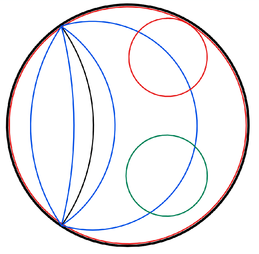
Figure 30: Circle (green), horocircles (red) and hypercircles (blue and black) in $H^{2}$ space. Those hypercircles share the same axis (black). They are symmetric under the reflection with respect to their axis.

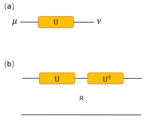
Figure 31: (a) Tensor $U$. (b) Tensor $U$ is proportional to an isometry.

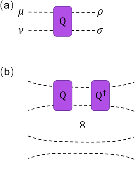
Figure 32: (a) Tensor $Q$, where two indexes on each side are grouped together. (b) Tensor $Q$ is proportional to the isometry between the two grouped indexes.

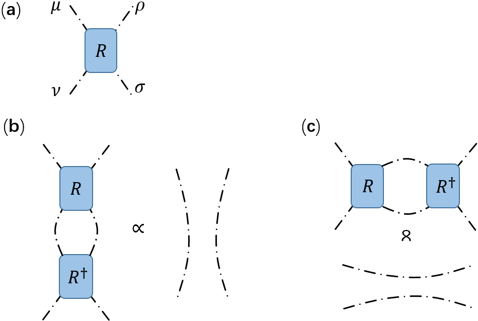
Figure 33: (a) Tensor $R$. (b) Tensor $R$ is proportional to isometries along two directions.

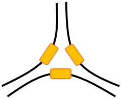
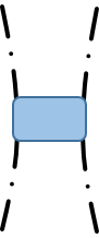
Figure 34: (a) Tensor $T$ and (b) Tensor $E$ for the tensor network with $\left\{7,3\right\}$ tiling and $S_{c}=\left\{\begin{bmatrix}[0.5]1\\ 3\end{bmatrix},\begin{bmatrix}[0.5]1&1\\ 1&1\end{bmatrix}\right\}$.

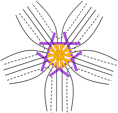
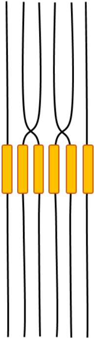
Figure 35: (a) Tensor $T$ and (b) Tensor $E$ for the tensor network with $\{4,5\}$ tiling and $S_{c}=\left\{\begin{bmatrix}[0.5]1\\ 4\end{bmatrix},\begin{bmatrix}[0.5]1&1&1\\ 3&2&3\end{bmatrix}\right\}$.

Appendix B Specific construction of tensors subject to tensor constraints

Analogous to the construction of tensors in Evenbly:2017htn and Ling:2018qec , we define tensors $U$, $Q$ and $R$ as the building blocks for tensors $T$ and $E$, as shown in Fig.33, 33 and 33. The elements of tensor $U$ are $U_{\mu\nu}$, which satisfy

$$U_{\mu\nu}=U_{\nu\mu},\quad\sum_{\nu}U_{\mu\nu}U_{\rho\nu}^{*}\propto\delta_{\mu\rho}.$$ (109)

The elements of tensor $Q$ are $Q_{\mu\nu\rho\sigma}$ which satisfy

$$Q_{\mu\nu\rho\sigma}=Q_{\rho\sigma\mu\nu}=Q_{\nu\mu\sigma\rho},\quad\sum_{\rho\sigma}Q_{\mu\nu\rho\sigma}Q_{\mu^{\prime}\nu^{\prime}\rho\sigma}^{*}\propto\delta_{\mu\mu^{\prime}}\delta_{\nu\nu^{\prime}}.$$ (110)

where two indexes $\mu\nu$ ($\rho\sigma$) are grouped together. The elements of tensor $R$ are $R_{\mu\nu\rho\sigma}$, which satisfy

$$R_{\mu\nu\rho\sigma}=R_{\rho\sigma\mu\nu}=R_{\nu\mu\sigma\rho},\quad\sum_{\rho\sigma}R_{\mu\nu\rho\sigma}R_{\mu^{\prime}\nu^{\prime}\rho\sigma}^{*}\propto\delta_{\mu\mu^{\prime}}\delta_{\nu\nu^{\prime}},\quad\sum_{\nu\sigma}R_{\mu\nu\rho\sigma}R_{\mu^{\prime}\nu\rho^{\prime}\sigma}^{*}\propto\delta_{\mu\mu^{\prime}}\delta_{\rho\rho^{\prime}}.$$ (111)

For the tensor network with $\left\{7,3\right\}$ tiling and $S_{c}=\left\{\begin{bmatrix}[0.5]1\\ 2\end{bmatrix},\begin{bmatrix}[0.5]1&1\\ 1&1\end{bmatrix}\right\}$, and the tensor network with $\{4,5\}$ tiling and $S_{c}=\left\{\begin{bmatrix}[0.5]1\\ 4\end{bmatrix},\begin{bmatrix}[0.5]1&1&1\\ 3&2&3\end{bmatrix}\right\}$, we construct tensors $T$ and $E$ in Fig.35 and 35, respectively. The specific structures of the top tensor chain in these two tensor networks are also shown in Fig.36.

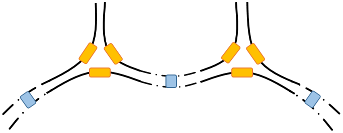
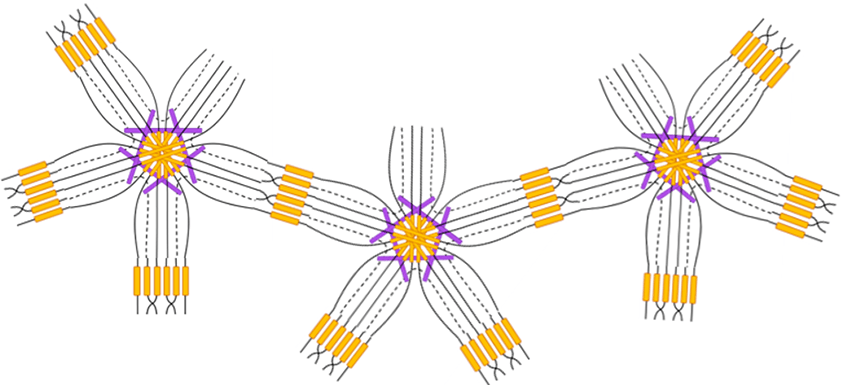
Figure 36: (a) The top tensor chain $\begin{bmatrix}[0.5]1&1\\ 2&2\end{bmatrix}$ in the tensor network with $\left\{7,3\right\}$ tiling and $S_{c}=\left\{\begin{bmatrix}[0.5]1\\ 2\end{bmatrix},\begin{bmatrix}[0.5]1&1\\ 1&1\end{bmatrix}\right\}$. (b) The top tensor chain $\begin{bmatrix}[0.5]1&1&1\\ 3&2&3\end{bmatrix}$ in the tensor network with $\{4,5\}$ tiling and $S_{c}=\left\{\begin{bmatrix}[0.5]1\\ 4\end{bmatrix},\begin{bmatrix}[0.5]1&1&1\\ 3&2&3\end{bmatrix}\right\}$.

References

- (1) G. Vidal, “Entanglement Renormalization,” Phys. Rev. Lett. 99, no. 22, 220405 (2007) [cond-mat/0512165].
- (2) S. Ryu and T. Takayanagi, “Holographic derivation of entanglement entropy from AdS/CFT,” Phys. Rev. Lett. 96, 181602 (2006) [hep-th/0603001].
- (3) B. Swingle, “Entanglement Renormalization and Holography,” Phys. Rev. D 86, 065007 (2012) [arXiv:0905.1317 [cond-mat.str-el]].
- (4) B. Swingle, “Constructing holographic spacetimes using entanglement renormalization,” arXiv:1209.3304 [hep-th].
- (5) M. Van Raamsdonk, “Building up spacetime with quantum entanglement,” Gen. Rel. Grav. 42, 2323 (2010) [Int. J. Mod. Phys. D 19, 2429 (2010)] [arXiv:1005.3035 [hep-th]].
- (6) J. M. Maldacena, “Eternal black holes in anti-de Sitter,” JHEP 0304, 021 (2003) [hep-th/0106112].
- (7) M. Nozaki, S. Ryu and T. Takayanagi, “Holographic Geometry of Entanglement Renormalization in Quantum Field Theories,” JHEP 1210, 193 (2012) [arXiv:1208.3469 [hep-th]].
- (8) X. L. Qi, “Exact holographic mapping and emergent space-time geometry,” arXiv:1309.6282 [hep-th].
- (9) B. Schumacher and M. A. Nielsen, “Quantum data processing and error correction,” Phys. Rev. A 54, 2629 (1996) [quant-ph/9604022].
- (10) A. Hamilton, D. N. Kabat, G. Lifschytz and D. A. Lowe, “Holographic representation of local bulk operators,” Phys. Rev. D 74, 066009 (2006) [hep-th/0606141].
- (11) X. Dong, D. Harlow and A. C. Wall, “Reconstruction of Bulk Operators within the Entanglement Wedge in Gauge-Gravity Duality,” Phys. Rev. Lett. 117, no. 2, 021601 (2016) [arXiv:1601.05416 [hep-th]].
- (12) D. Harlow, “TASI Lectures on the Emergence of the Bulk in AdS/CFT,” arXiv:1802.01040 [hep-th].
- (13) J. Cotler, P. Hayden, G. Salton, B. Swingle and M. Walter, “Entanglement Wedge Reconstruction via Universal Recovery Channels,” arXiv:1704.05839 [hep-th].
- (14) A. Almheiri, X. Dong and D. Harlow, “Bulk Locality and Quantum Error Correction in AdS/CFT,” JHEP 1504, 163 (2015) [arXiv:1411.7041 [hep-th]].
- (15) E. Mintun, J. Polchinski and V. Rosenhaus, “Bulk-Boundary Duality, Gauge Invariance, and Quantum Error Corrections,” Phys. Rev. Lett. 115, no. 15, 151601 (2015) [arXiv:1501.06577 [hep-th]].
- (16) B. Freivogel, R. Jefferson and L. Kabir, “Precursors, Gauge Invariance, and Quantum Error Correction in AdS/CFT,” JHEP 1604, 119 (2016) [arXiv:1602.04811 [hep-th]].
- (17) D. Harlow, “The Ryu-Takayanagi Formula from Quantum Error Correction,” Commun. Math. Phys. 354, no. 3, 865 (2017) [arXiv:1607.03901 [hep-th]].
- (18) F. Pastawski, B. Yoshida, D. Harlow and J. Preskill, “Holographic quantum error-correcting codes: Toy models for the bulk/boundary correspondence,” JHEP 1506, 149 (2015) [arXiv:1503.06237 [hep-th]].
- (19) P. Hayden, S. Nezami, X. L. Qi, N. Thomas, M. Walter and Z. Yang, “Holographic duality from random tensor networks,” JHEP 1611, 009 (2016) [arXiv:1601.01694 [hep-th]].
- (20) A. Bhattacharyya, Z. S. Gao, L. Y. Hung and S. N. Liu, “Exploring the Tensor Networks/AdS Correspondence,” JHEP 1608, 086 (2016) [arXiv:1606.00621 [hep-th]].
- (21) X. L. Qi and Z. Yang, “Space-time random tensor networks and holographic duality,” arXiv:1801.05289 [hep-th].
- (22) Z. Yang, P. Hayden and X. L. Qi, “Bidirectional holographic codes and sub-AdS locality,” JHEP 1601, 175 (2016) [arXiv:1510.03784 [hep-th]].
- (23) G. Chirco, D. Oriti and M. Zhang, “Ryu-Takayanagi Formula for Symmetric Random Tensor Networks,” arXiv:1711.09941 [hep-th].
- (24) M. Han and S. Huang, “Discrete gravity on random tensor network and holographic Renyi entropy,” JHEP 1711, 148 (2017) [arXiv:1705.01964 [hep-th]].
- (25) G. Evenbly, “Hyper-invariant tensor networks and holography,” Phys. Rev. Lett. 119, 141602 [arXiv:1704.04229 [cond-mat, physics:quant-ph]].
- (26) M. Han and L. Y. Hung, “Loop Quantum Gravity, Exact Holographic Mapping, and Holographic Entanglement Entropy,” Phys. Rev. D 95, no. 2, 024011 (2017) [arXiv:1610.02134 [hep-th]].
- (27) P. Calabrese and J. L. Cardy, “Entanglement entropy and quantum field theory,” J. Stat. Mech. 0406, P06002 (2004) [hep-th/0405152].
- (28) P. Calabrese and J. Cardy, “Entanglement entropy and conformal field theory,” J. Phys. A 42, 504005 (2009) [arXiv:0905.4013 [cond-mat.stat-mech]].
- (29) I. H. Kim and M. J. Kastoryano, “Entanglement renormalization, quantum error correction, and bulk causality,” JHEP 1704, 040 (2017) [arXiv:1701.00050 [quant-ph]].
- (30) N. Bao, C. Cao, S. M. Carroll, A. Chatwin-Davies, N. Hunter-Jones, J. Pollack and G. N. Remmen, “Consistency conditions for an AdS multiscale entanglement renormalization ansatz correspondence,” Phys. Rev. D 91, no. 12, 125036 (2015) [arXiv:1504.06632 [hep-th]].
- (31) W. Donnelly, B. Michel, D. Marolf and J. Wien, “Living on the Edge: A Toy Model for Holographic Reconstruction of Algebras with Centers,” JHEP 1704, 093 (2017) [arXiv:1611.05841 [hep-th]].
- (32) Y. Ling, Y. Liu, Z. Y. Xian and Y. Xiao, “Quantum error correction and entanglement spectrum in tensor network,”. [arXiv:1806.05007 [hep-th]].
- (33) B. Schumacher, and M. D. Westmoreland, “Approximate Quantum Error Correction,” Quantum Information Processing 1, 5–12 (2002) [arXiv:quant-ph/0112106].
- (34) S. T. Flammia, J. Haah, M. J. Kastoryano and I. H. Kim, “Limits on the storage of quantum information in a volume of space,” Quantum 1, 4 (2017) [arXiv:1610.06169 [quant-ph]].
- (35) T. Jacobson, “Entanglement Equilibrium and the Einstein Equation,” Phys. Rev. Lett. 116, no. 20, 201101 (2016) [arXiv:1505.04753 [gr-qc]].
- (36) X. Dong, “The Gravity Dual of Renyi Entropy,” Nature Commun. 7, 12472 (2016) [arXiv:1601.06788 [hep-th]].