Matter parametric neutrino flavor transformation through Rabi resonances

Abstract

We consider the flavor transformation of neutrinos through oscillatory matter profiles. We show that the neutrino oscillation Hamiltonian in this case describes a Rabi system with an infinite number of Rabi modes. We further show that, in a given physics problem, the majority of the Rabi modes have too small amplitudes to be relevant. We also go beyond the rotating wave approximation and derive the relative detuning of the Rabi resonance when multiple Rabi modes with small amplitudes are present. We provide an explicit criterion of whether an off-resonance Rabi mode can affect the parametric flavor transformation of the neutrino.

I Introduction

Neutrinos are constantly produced by stars, and they are also emitted much more intensively during the violent deaths of massive stars through core-collapse supernovae albeit for only a brief moment. The neutrinos from stellar objects and other astronomical sources provide a unique probe to observe these objects and to study the properties of the neutrinos themselves (see, e.g., Refs Robertson:2012ib ; Mirizzi:2015eza for reviews on solar neutrinos and supernova neutrinos). The interpretation of the neutrino signals from astronomical sources depends on the understanding of the flavor transformation or oscillations of the neutrinos. A well-known mechanism for a neutrino to experience flavor transformation is the Mikheyev-Smirnov-Wolfenstein (MSW) effect when the neutrino propagate through a region where the matter density varies smoothly across a critical value Wolfenstein:1977ue ; Mikheyev:1985aa . Inside the stars and supernovae the matter densities may have rapid changes and fluctuations which can also leave important imprints on the passing-through neutrinos Haxton:1990qb ; Sawyer:1990tw ; Nunokawa:1996qu ; Burgess:1996mz ; Sawyer:1990tw ; Loreti:1995ae ; Friedland:2006ta ; Fogli:2006xy ; Kneller:2010sc ; Choubey:2007ga . In an extreme case supernova neutrinos can become completely flavor depolarized as they traverse the turbulent region behind the supernova shock Friedland:2006ta .

A matter profile with density fluctuations can cause neutrino flavor conversion through parametric resonances even when the matter density never crosses the critical value (see, e.g., Ref. Akhmedov:1999ty for a review). For example, a neutrino can achieve a maximum flavor conversion if the matter density varies sinusoidally on a length scale which matches that of the neutrino oscillation in matter with the mean density Krastev:1989ix . Using the Jacobi-Anger expansion and the rotating wave approximation Kneller et al have shown that a parametric resonance can also occur when the neutrino oscillation frequency with the mean matter density matches a harmonic of the spatial frequency of the sinusoidal matter fluctuation Kneller:2012id . This result has been generalized to the scenarios with matter fluctuations of multiple Fourier modes Patton:2013dba , slowly varying base profiles Patton:2014lza and three-flavor neutrino mixing Yang:2015oya .

The existence of harmonic parametric resonances is an intriguing phenomenon, but its physical origin is somewhat buried in the mathematical procedure employed in Ref. Kneller:2012id . It is not entirely clear why the flavor transformation of the neutrino can be described by only a handful parametric resonances although there can exist many more such resonances Patton:2014lza . There also lacks a criterion of when the rotating wave approximation fails. We intend to address these issues in this short paper. We will not consider the collective flavor transformation of the neutrinos due to the neutrino self-refraction (see, e.g., Refs. Duan:2010bg ; Chakraborty:2016yeg for reviews on this interesting subject).

The rest of the paper is organized as follows. In Sec. II we will show that the neutrino oscillation Hamiltonian with an oscillatory matter profile have an infinite number of Rabi modes which produce the harmonic parametric resonances. In Sec. III we will demonstrate that only a finite number, usually a small portion, of the Rabi modes are relevant in a physical situation. We will also derive a quantitative criterion of when an off-resonance Rabi mode may significantly affect the parametric resonance. In Sec. IV we will summarize and conclude our work.

II Rabi resonances in oscillatory matter profiles

II.1 Equation of motion

As in Ref. Patton:2013dba we will consider the mixing between two (effective) neutrino flavors $\nu_{e}$ and $\nu_{x}$. The flavor wavefunction of the neutrino in flavor basis is $\Psi^{(\mathrm{f})}=[\psi_{\nu_{e}},\psi_{\nu_{x}}]^{T}$, where $\psi_{\nu_{\alpha}}=\langle\nu_{\alpha}|\psi\rangle$ ($\alpha=e,x$) is the amplitude for the neutrino in state $|\psi\rangle$ to be found in $|\nu_{\alpha}\rangle$, and $|\psi_{\nu_{e}}|^{2}+|\psi_{\nu_{x}}|^{2}=1$. The flavor evolution of the neutrino in matter is described by the Schrödinger equation

$$\mathrm{i}\frac{\mathrm{d}}{\mathrm{d}r}\Psi^{(\mathrm{f})}(r)=\mathsf{H}^{(\mathrm{f})}\Psi^{(\mathrm{f})}(r),$$ (1)

where the neutrino oscillation Hamiltonian is

$$\mathsf{H}^{(\mathrm{f})}=[-\omega_{\mathrm{v}}\cos(2\theta_{\mathrm{v}})+\lambda(r)]\frac{\sigma_{3}}{2}+\omega_{\mathrm{v}}\sin(2\theta_{\mathrm{v}})\frac{\sigma_{1}}{2}.$$ (2)

In the above equation, $\omega_{\mathrm{v}}$ and $\theta_{\mathrm{v}}$ are the oscillation frequency and the mixing angle of the neutrino in vacuum, respectively, $\sigma_{i}$ ($i=1,2,3$) are the Pauli matrices, and $\lambda(r)=\sqrt{2}G_{\mathrm{F}}n_{e}(r)$ is the matter potential at a distance $r$ along the neutrino propagation trajectory, where $G_{\mathrm{F}}$ is the Fermi coupling constant, and $n_{e}$ the net electron number density. In Eq. (1) we have ignored the trace term of the Hamiltonian which does not affect neutrino oscillations. Throughout the paper we adopt the natural units with $\hbar=c=1$.

In this work we will assume a stationary matter profile of the form

$$\lambda(r)=\lambda_{0}+\delta\lambda(r),$$ (3)

where $\delta\lambda(r)$ is a small perturbation to the uniform background matter potential $\lambda_{0}$. As in Refs. Kneller:2012id ; Patton:2013dba we define the background matter basis

$$|\nu^{(\mathrm{m})}_{1}\rangle =\cos\theta_{\mathrm{m}}|\nu_{e}\rangle-\sin\theta_{\mathrm{m}}|\nu_{x}\rangle,$$ (4a)

$$|\nu^{(\mathrm{m})}_{2}\rangle =\sin\theta_{\mathrm{m}}|\nu_{e}\rangle+\cos\theta_{\mathrm{m}}|\nu_{x}\rangle,$$ (4b)

where

$$\theta_{\mathrm{m}}=\frac{1}{2}\arctan\left(\frac{\omega_{\mathrm{v}}\sin(2\theta_{\mathrm{v}})}{\omega_{\mathrm{v}}\cos(2\theta_{\mathrm{v}})-\lambda_{0}}\right).$$ (5)

The Hamiltonian in the background matter basis is

$$\mathsf{H}^{(\mathrm{m})}=-[\omega_{\mathrm{m}}-\cos(2\theta_{\mathrm{m}})\delta\lambda]\frac{\sigma_{3}}{2}+\sin(2\theta_{\mathrm{m}})\delta\lambda\frac{\sigma_{1}}{2},$$ (6)

where

$$\omega_{\mathrm{m}}=\sqrt{[\omega_{\mathrm{v}}\cos(2\theta_{\mathrm{v}})-\lambda_{0}]^{2}+[\omega_{\mathrm{v}}\sin(2\theta_{\mathrm{v}})]^{2}}$$ (7)

is the neutrino oscillation frequency in matter when $\delta\lambda=0$.

For definiteness we will use $\sin^{2}(2\theta_{\mathrm{v}})=0.093$ in all the numerical examples shown later in the paper. We will also assume that the background matter density is a quarter of the value of the MSW resonance, i.e.  $\lambda_{0}=\frac{1}{4}\omega_{\mathrm{v}}\cos(2\theta_{\mathrm{v}})$. These values and the amplitudes of the matter fluctuations are chosen to illustrate the general principles to be discussed in this paper and do not necessarily reflect the actual conditions in real physical problems.

II.2 Rabi resonance

We first consider a sinusoidal matter perturbation of amplitude $\lambda^{\prime}\ll\omega_{\mathrm{m}}$ and wave number $k$:

$$\delta\lambda(r)=\lambda^{\prime}\cos(kr).$$ (8)

Because the fluctuation amplitude is small, we will drop the perturbation in the diagonal terms in Eq. (6) as a first order approximation so that

$$\mathsf{H}^{(\mathrm{m})}\approx\frac{1}{2}\begin{bmatrix}-\omega_{\mathrm{m}}&\sum_{n=\pm 1}A_{n}e^{\mathrm{i}K_{n}r}\\ \sum_{n=\pm 1}A_{n}e^{-\mathrm{i}K_{n}r}&\omega_{\mathrm{m}}\end{bmatrix}$$ (9)

where

$$K_{\pm 1} =\pm k$$ (10a)

and

$$A_{1} =A_{-1}=\frac{\sin(2\theta_{\mathrm{m}})\lambda^{\prime}}{2}.$$ (10b)

Eq. (9) has the same form as the equation of motion of a magnetic dipole in the presence of a magnetic field with two components, a constant component in the vertical direction and an oscillating component in the horizontal direction. The transition amplitude between the up and down states of the dipole can reach $100\%$ at the Rabi resonance where $k=\omega_{\mathrm{m}}$ (see, e.g., Ref. sakurai2011modern ).

It turns out that the neutrino flavor transformation Hamiltonian with an oscillatory density profile can always be cast into the form in Eq. (9). We will call each term in the sum of the off-diagonal element in Eq. (9) a “Rabi mode” with $A_{n}$ and $K_{n}$ being the amplitude and wave number of the corresponding Rabi mode. When the Rabi resonance condition

$$K_{n}=\omega_{\mathrm{m}}$$ (11)

is approximately satisfied, the transition probability of the neutrino between $|\nu^{(\mathrm{m})}_{1}\rangle$ and $|\nu^{(\mathrm{m})}_{2}\rangle$ takes the form

$$P\approx\frac{\sin^{2}(\Omega r/2)}{1+D_{n}^{2}},$$ (12)

where

$$D_{n}=\left|\frac{K_{n}-\omega_{\mathrm{m}}}{A_{n}}\right|$$ (13)

is the relative detuning of the Rabi mode, and

$$\Omega=A_{n}\sqrt{1+D_{n}^{2}}$$ (14)

is the Rabi frequency.

The relative detuning $D_{n}$ is a measure of how much the corresponding Rabi mode is away from its resonance. The Rabi mode $n$ is on resonance if $D_{n}\lesssim 1$ and is off resonance if $D_{n}\gg 1$. Because $D_{-1}>\omega_{\mathrm{m}}/\lambda^{\prime}\gg 1$, the $n=-1$ mode is always off resonance and is ignored by the rotating wave approximation.

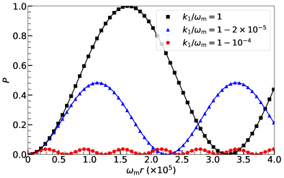
Figure 1: The transition probabilities $P$ between the two background matter states $|\nu^{(\mathrm{m})}_{1}\rangle$ and $|\nu^{(\mathrm{m})}_{2}\rangle$ of the neutrino as functions of distance $r$ for three matter profiles all of the form $\lambda(r)=\lambda_{0}+\lambda^{\prime}\cos(kr)$. The different symbols represent the numerical solutions to the Schrödinger equation with various values of $k$ as labeled. The continuous curves are obtained by using the Rabi formula in Eq. (12) and ignoring the off-resonance Rabi mode. In all three cases $\lambda^{\prime}/\omega_{\mathrm{m}}=10^{-4}$.

In Fig. 1 we compare the numerical solutions to the Schrödinger equation and the results obtained by applying the Rabi formula in Eq. (12) (with $n=1$) for three matter profiles with sinusoidal fluctuations of various wave numbers. The good agreement between the two sets of solutions justifies the approximations that we have made.

II.3 Jacobi-Anger expansion

The neutrino oscillation Hamiltonian in Eq. (6) actually contains an infinite number of Rabi modes even for a matter profile with a single Fourier mode. To see this we define a rotated matter basis:

$$|\tilde{\nu}_{1}\rangle =e^{\mathrm{i}\eta(r)}|\nu^{(\mathrm{m})}_{1}\rangle, |\tilde{\nu}_{2}\rangle =e^{-\mathrm{i}\eta(r)}|\nu^{(\mathrm{m})}_{2}\rangle,$$ (15)

where

$$\eta(r)-\eta(0)=\frac{\cos(2\theta_{\mathrm{m}})}{2}\int^{r}_{0}\delta\lambda(r^{\prime})\,\mathrm{d}r^{\prime}.$$ (16)

We note that the transition probability between $|\tilde{\nu}_{1}\rangle$ and $|\tilde{\nu}_{2}\rangle$ is the same as that between $|\nu^{(\mathrm{m})}_{1}\rangle$ and $|\nu^{(\mathrm{m})}_{2}\rangle$. The Hamiltonian in the rotated matter basis is

$$\widetilde{\mathsf{H}}=\frac{1}{2}\begin{bmatrix}-\omega_{\mathrm{m}}&\sin(2\theta_{\mathrm{m}})\delta\lambda e^{2\mathrm{i}\eta}\\ \sin(2\theta_{\mathrm{m}})\delta\lambda e^{-2\mathrm{i}\eta}&\omega_{\mathrm{m}}\end{bmatrix}.$$ (17)

For the sinusoidal matter perturbation $\delta\lambda=\lambda^{\prime}\cos(kr)$ we take $\eta(r)=\cos(2\theta_{\mathrm{m}})\lambda^{\prime}\sin(kr)/2k$ and apply the Jacobi-Anger expansion as in Ref. Kneller:2012id

$$e^{\mathrm{i}z\sin\xi}=\sum_{n=-\infty}^{\infty}J_{n}(z)e^{\mathrm{i}n\xi},$$ (18)

where $J_{n}(z)$ is the $n$th Bessel function of the first kind. Utilizing the identity

$$J_{n-1}(z)+J_{n+1}(z)=\frac{2n}{z}J_{n}(z)$$ (19)

we obtain

$$\lambda^{\prime}\cos(kr)e^{2\mathrm{i}\eta} =\frac{\lambda^{\prime}}{2}(e^{\mathrm{i}kr}+e^{-\mathrm{i}kr})\sum_{n=-\infty}^{\infty}J_{n}(u)e^{\mathrm{i}nkr}$$

$$=\frac{1}{\cos(2\theta_{\mathrm{m}})}\sum_{n=-\infty}^{\infty}nkJ_{n}(u)e^{\mathrm{i}nkr},$$ (20)

where $u=\cos(2\theta_{\mathrm{m}})\lambda^{\prime}/k$. Therefore, the Hamiltonian in the rotated matter basis indeed has a form similar to Eq. (9) but with an infinite number of Rabi modes:

$$\widetilde{\mathsf{H}}=\frac{1}{2}\begin{bmatrix}-\omega_{\mathrm{m}}&\sum_{n}A_{n}e^{\mathrm{i}K_{n}r}\\ \sum_{n}A_{n}e^{-\mathrm{i}K_{n}r}&\omega_{\mathrm{m}}\end{bmatrix}$$ (21)

where $n=0,\pm 1,\pm 2,\cdots$,

$$K_{n} =nk,$$ (22a)

and

$$A_{n} =\tan(2\theta_{\mathrm{m}})K_{n}J_{n}(u).$$ (22b)

Eqs. (11) and (12) show that a parametric resonance occurs when $\omega_{\mathrm{m}}$ matches a harmonic of the spatial frequency of the sinusoidal matter fluctuation.

When the $n=1$ mode is approximately on resonance,

$$A_{1}\xrightarrow{k\approx\omega_{\mathrm{m}}\gg\lambda^{\prime}}\frac{\sin(2\theta_{\mathrm{m}})\lambda^{\prime}}{2}$$

which reduces to Eq. (10b). Here we have used the asymptotic form of the Bessel function

$$J_{n}(z)\xrightarrow{z\ll\sqrt{n+1}}\frac{(z/2)^{n}}{n!}\quad\text{if }n>0.$$ (23)

In applying the Rabi formula in Eq. (12) one has assumed the rotating wave approximation and ignored all the off-resonance Rabi modes.

II.4 Multiple Fourier modes

Now we consider the scenario where the matter fluctuation has multiple Fourier modes:

$$\delta\lambda(r)=\sum_{a}\lambda_{a}\cos(k_{a}r+\phi_{a}),$$ (24)

where $\lambda_{a}$, $k_{a}$ and $\phi_{a}$ are the amplitude, wave number and initial phase of the $a$th Fourier mode, respectively. Using the same technique as that in Sec. II.3 one can show that

$$\widetilde{\mathsf{H}}=\frac{1}{2}\begin{bmatrix}-\omega_{\mathrm{m}}&\sum_{\mathcal{N}}A_{\mathcal{N}}e^{\mathrm{i}(K_{\mathcal{N}}r+\Phi_{\mathcal{N}})}\\ \sum_{\mathcal{N}}A_{\mathcal{N}}e^{-\mathrm{i}(K_{\mathcal{N}}r+\Phi_{\mathcal{N}})}&\omega_{\mathrm{m}}\end{bmatrix},$$ (25)

where the sum is over all possible choices of $\mathcal{N}=\{\cdots,n_{a},\cdots\}$ with $n_{a}$ being an arbitrary integer associated with the $a$th Fourier mode, and

$$K_{\mathcal{N}} =\sum_{a}n_{a}k_{a},$$ (26a)

$$\Phi_{\mathcal{N}} =\sum_{a}n_{a}\phi_{a},$$ (26b)

and

$$A_{\mathcal{N}} =\tan(2\theta_{\mathrm{m}})K_{\mathcal{N}}\prod_{a}J_{n_{a}}(u_{a})$$ (26c)

are the wave number, initial phase and amplitude of the Rabi mode $\mathcal{N}$ with

$$u_{a} =\frac{\cos(2\theta_{\mathrm{m}})\lambda_{a}}{k_{a}}.$$ (27)

Therefore, one expects that the flavor transformation of the neutrino is enhanced when the Rabi resonance condition

$$K_{\mathcal{N}}=\omega_{\mathrm{m}}$$ (28)

is approximately met. We note that the resonance condition is independent of the initial phases of the Rabi modes.

III Further discussion on Rabi resonances

III.1 Amplitudes of the Rabi modes

The physics prescription presented in Sec. II.4 seems simple and appealing, but there remain a few questions that need to be answered. First and foremost, there can exist many Fourier modes in a realistic matter profile. If $\lambda_{0}(r)$ is a slowly varying function of distance $r$ (as in most realistic cases), at any given point one can almost always find some or even many choices of $\mathcal{N}$ with which the resonance condition in Eq. (28) is approximately satisfied. And yet Patton et al found that only a few resonances were needed to account for the neutrino flavor transformation through (at least some of) the matter profiles in supernovae Patton:2014lza . They proposed that a parametric resonance is applicable only when the density scale height

$$h(r)=\lambda_{0}\left|\frac{\mathrm{d}\lambda_{0}}{\mathrm{d}r}\right|^{-1}$$ (29)

is longer than the length scale of the Rabi transition, or

$$\Omega h\gtrsim 1.$$ (30)

This criterion makes physical sense because we have assumed $\lambda_{0}$ to be constant in Sec. II.4 which is approximately true on the length scale of $h$.

Here we would like to point out that, even if many harmonic parametric resonances may exist for a given oscillatory matter profile, only a finite number, probably just a few, of them are relevant in a physical problem. The reason is the following. The Rabi oscillation frequency is determined by the Rabi mode $R$ that is (approximately) on resonance, i.e., $\Omega\approx A_{R}$. Using Eqs. (23) and (26c) and identity $J_{-n}(z)=(-1)^{n}J_{n}(z)$ we obtain

$$A_{R}\sim\omega_{\mathrm{m}}\tan(2\theta_{\mathrm{m}})\sideset{}{{}^{\prime}}{\prod}_{a}\left(\frac{\lambda_{a}}{k_{a}}\right)^{|n_{a}|}\sideset{}{{}^{\prime\prime}}{\prod}_{b}J_{n_{b}}(u_{b})$$ (31)

where $\prod^{\prime}$ includes all the “regular” Fourier modes with $\lambda_{a}/k_{a}\ll 1$, and $\prod^{\prime\prime}$ includes the rest of the Fourier modes. One expects that most of the Fourier modes are regular if the fluctuation amplitude of the matter profile is small. We will call $|n_{a}|$ the “order of contribution” to the Rabi mode $R$ by the $a$th Fourier mode. A Fourier mode is “standby” if $n_{a}=0$ and “participating” otherwise. From Eq. (31) one sees that, there can be only a few participating, regular Fourier modes and the order of contribution of each of these Fourier modes must be small. Otherwise, the amplitude $A_{R}$ of the Rabi mode will be too small to be relevant. If, however, the amplitude of a Fourier mode $b$ is so large or its wavelength is so long (but is still shorter than $h$ or the physical size of the system) that $\lambda_{b}/k_{b}\gtrsim 1$, then, according to Eq. (23), it can contribute to the Rabi mode up to the order of $|n_{b}|\lesssim(\lambda_{b}/k_{b})^{2}$ or the amplitude of the Rabi mode will be again too small to be relevant.

The above constraints on the contribution orders of the Fourier modes put a stringent limit on the number of the on-resonance Rabi modes that one needs to consider in a real physical problem.

III.2 Interference between Rabi modes

The Rabi formula in Eq. (12) was derived assuming that there exists only one Rabi mode. In Refs. Kneller:2012id ; Patton:2013dba ; Patton:2014lza the rotating wave approximation was employed which is equivalent to ignoring all the Rabi modes that are off-resonance. However, under certain conditions the rotating wave approximation may fail, and off-resonance Rabi modes can interfere with the on-resonance mode as we will show below.

We first consider a Rabi system with an on-resonance mode $R$ and an off-resonance mode $O$. The Hamiltonian of the system is the same as that in Eq. (25) except with $\mathcal{N}=R$ and $O$ only. We define a new basis

$$\begin{bmatrix}|\nu^{\prime}_{1}\rangle\\ |\nu^{\prime}_{2}\rangle\end{bmatrix}=\begin{bmatrix}\cos\Theta&-\sin\Theta\\ \sin\Theta&\cos\Theta\end{bmatrix}\begin{bmatrix}e^{-\mathrm{i}(K_{O}r+\Phi_{O})/2}|\tilde{\nu}_{1}\rangle\\ e^{\mathrm{i}(K_{O}r+\Phi_{O})/2}|\tilde{\nu}_{2}\rangle\end{bmatrix},$$ (32)

where

$$\Theta =\frac{1}{2}\arctan\left(\frac{A_{O}}{\omega_{\mathrm{m}}-K_{O}}\right).$$ (33)

The Hamiltonian in this new basis is

$$\mathsf{H}^{\prime}=\frac{1}{2}\begin{bmatrix}-\omega_{\mathrm{m}}^{\prime}-A_{R}\cos(\Upsilon(r))\sin(2\Theta)&A_{R}(e^{\mathrm{i}\Upsilon(r)}\cos^{2}\Theta-e^{-\mathrm{i}\Upsilon(r)}\sin^{2}\Theta)\\ A_{R}(e^{-\mathrm{i}\Upsilon(r)}\cos^{2}\Theta-e^{\mathrm{i}\Upsilon(r)}\sin^{2}\Theta)&\omega_{\mathrm{m}}^{\prime}+A_{R}\cos(\Upsilon(r))\sin(2\Theta)\end{bmatrix}$$ (34)

where

$$\omega_{\mathrm{m}}^{\prime} =\text{sgn}(\omega_{\mathrm{m}}-K_{O})\sqrt{(\omega_{\mathrm{m}}-K_{O})^{2}+A_{O}^{2}}$$ (35)

and

$$\Upsilon(r)=(K_{R}+K_{O})r+\Phi_{R}+\Phi_{O}.$$ (36)

Because $A_{R}$ is small, we will keep only the off-diagonal oscillatory terms in $\mathsf{H}^{\prime}$ that are approximately on resonance so that

$$\mathsf{H}^{\prime}\approx\frac{1}{2}\begin{bmatrix}-\omega_{\mathrm{m}}^{\prime}&A_{R}e^{\mathrm{i}\Upsilon(r)}\\ A_{R}e^{-\mathrm{i}\Upsilon(r)}&\omega_{\mathrm{m}}^{\prime}\end{bmatrix}.$$ (37)

This is exactly the Hamiltonian for a single-mode Rabi system. Therefore, a resonance occurs when

$$K_{R}=\omega_{\mathrm{m}}^{\prime}=\omega_{\mathrm{m}}+\Delta\omega_{\mathrm{m}}$$ (38)

where

$$\Delta\omega_{\mathrm{m}}=\omega_{\mathrm{m}}^{\prime}-(\omega_{\mathrm{m}}-K_{O})\approx\frac{A_{O}^{2}/2}{\omega_{\mathrm{m}}-K_{O}}.$$ (39)

Comparing Eqs. (28) and (38) one sees that the resonance frequency is shifted by $\Delta\omega_{\mathrm{m}}$ because of the off-resonance mode. This shift of the resonance frequency due to the off-resonance Rabi modes is known as the ac Stark effect (see, e.g., Ref. Cohen-Tannoudji:1996 ). The new relative detuning of the Rabi system is

$$D^{\prime}_{R}=\left|\frac{K_{R}-(\omega_{\mathrm{m}}+\Delta\omega_{\mathrm{m}})}{A_{R}}\right|.$$ (40)

The off-resonance mode will have a significant impact on the resonance if the change of the relative detuning

$$\Delta D_{R}=|D^{\prime}_{R}-D_{R}|=\left|\frac{\Delta\omega_{\mathrm{m}}}{A_{R}}\right|$$ (41)

is of order 1 or larger, or, equivalently,

$$|A_{O}|\gtrsim\sqrt{2|A_{R}(\omega_{\mathrm{m}}-K_{O})|}\sim\sqrt{|A_{R}|\omega_{\mathrm{m}}}.$$ (42)

This explains why the off-resonance Rabi modes can be ignored in the case with a single Fourier mode (see Fig. 1). When the $n=1$ mode is almost on resonance, the $n=-1$ mode does not satisfies the criterion in Eq. (42) because $A_{-1}=A_{1}\ll\omega_{\mathrm{m}}$. The Rabi modes with $|n|>1$ have even smaller amplitudes than the $n=-1$ mode.

We note that the Rabi system with two Rabi modes describes a magnetic dipole in the presence of three magnetic fields: $\mathbf{B}_{0}$ in the $z$ direction which corresponds to the diagonal elements of the Hamiltonian $\mathsf{H}$, and $\mathbf{B}_{R}$ and $\mathbf{B}_{O}$ which rotate in the $x$-$y$ plane with different angular frequencies $K_{R}$ and $K_{O}$ and which correspond the two Rabi modes in the off-diagonal element of $\mathsf{H}$. The essence of Eqs. (32) and (34) is to transform the equation of motion from the static frame to the reference frame which co-rotates with $\mathbf{B}_{O}$. In this rotating frame one has only one rotating field $\mathbf{B}_{R}^{\prime}$ and one static field $\mathbf{B}_{0}^{\prime}+\mathbf{B}_{O}^{\prime}$, where the primes indicate the quantities in the rotating frame. The static field $\mathbf{B}_{0}^{\prime}+\mathbf{B}_{O}^{\prime}$ is titled away from the $z$ axis by an angle $2\Theta$.. Because we consider the scenarios where all the rotating fields have amplitudes much smaller than $|\mathbf{B}_{0}|$, $\Theta$ is small and can be ignored. Therefore, the system in the co-rotating frame corresponds to a Rabi system with only one Rabi mode $\mathbf{B}_{R}^{\prime}$ the properties of which are given by Eqs. (12), (13) and (14). The interference effect due to the off-resonance Rabi mode $\mathbf{B}_{O}$ is manifested in the change of the magnitude of the static field $|\mathbf{B}_{0}|\rightarrow|\mathbf{B}_{0}^{\prime}+\mathbf{B}_{O}^{\prime}|$.

For a Rabi system with one on-resonance Rabi mode and two off-resonance Rabi modes all of which have small amplitudes, one can transform the equation of motion to the reference frame which co-rotates with one of the off-resonance mode. In this reference frame there are only two Rabi modes and the energy gap $\omega_{\mathrm{m}}$ changes to $\omega_{\mathrm{m}}^{\prime}$. One can then applies the results of the two-mode Rabi system that we discussed above. In general, for a Rabi system with $N$ small-amplitude Rabi modes, one can always go to the reference frame that co-rotates with one of the off-resonance Rabi mode. In this co-rotating frame the number of Rabi modes is reduced by one, and one can apply the results of the Rabi system with $N-1$ modes. Using the reduction procedure we find that, for the scenario with one on-resonance Rabi mode and many off-resonance modes, Eq. (39) is generalized to

$$\Delta\omega_{\mathrm{m}}\approx\sum_{O}\frac{A_{O}^{2}/2}{\omega_{\mathrm{m}}-K_{O}},$$ (43)

where the summation is carried over all the off-resonance Rabi modes. In particular, if only a pair of off-resonance Rabi modes $O_{\pm}$ have large enough amplitudes to affect the resonance, and if $A_{O_{+}}=A_{O_{-}}$ and $K_{O_{+}}=-K_{O_{-}}$, we have

$$\Delta\omega_{\mathrm{m}}\approx\frac{A_{O+}^{2}\omega_{\mathrm{m}}}{\omega_{\mathrm{m}}^{2}-K_{O_{+}}^{2}}.$$ (44)

The relative detuning of the multi-mode Rabi system is still given by Eq. (40).

As a concrete example we consider a matter profile of two Fourier modes:

$$\lambda(r)=\lambda_{0}+\lambda_{1}\cos(k_{1}r)+\lambda_{2}\sin(k_{2}r).$$ (45)

We choose $k_{1}=\omega_{\mathrm{m}}$ so that the Rabi mode $R=\{1,0\}$ is exactly on resonance. We choose the second Fourier mode to have a long wavelength ($k_{2}=0.1\omega_{\mathrm{m}}$) and a relatively large amplitude ($\lambda_{2}=320\lambda_{1}=3.2\times 10^{-2}\omega_{\mathrm{m}}$). We compute the transition probability $P$ between $|\nu_{1}^{(\mathrm{m})}\rangle$ and $|\nu_{2}^{(\mathrm{m})}\rangle$ as a function of distance $r$ by solving the Schrödinger equation numerically, and the result is shown in Fig. 2. As comparison we also show in the same figure the transition probabilities predicted by the Rabi formula when only the on-resonance Rabi mode $R=\{1,0\}$ is included, both the $R$ mode and an off-resonance mode $O_{+}=\{0,1\}$ are included, and the $R$ mode and two off-resonance modes $O_{+}$ and $O_{-}=\{0,-1\}$ are included, respectively. One can see that the numerical solution agrees very well with the prediction based on the Rabi formula when three Rabi modes $R$ and $O_{\pm}$ are included. One can also see that the two long-wavelength, off-resonance Rabi modes $O_{\pm}$ combine to suppress the Rabi transition.

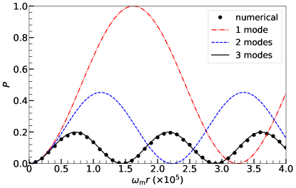
Figure 2: Similar to Fig. 1 but for a matter profile of the form $\lambda(r)=\lambda_{0}+\lambda_{1}\cos(k_{1}r)+\lambda_{2}\sin(k_{2}r)$, where $\lambda_{1}/\omega_{\mathrm{m}}=10^{-4}$, $k_{1}/\omega_{\mathrm{m}}=1$, $\lambda_{2}/\omega_{\mathrm{m}}=3.2\times 10^{-2}$ and $k_{2}/\omega_{\mathrm{m}}=0.1$. The filled circles represent the numerical solution to the Schrödinger equation, and the continuous curves represent the predictions by the Rabi formula when 1, 2 and 3 Rabi modes are included, respectively.

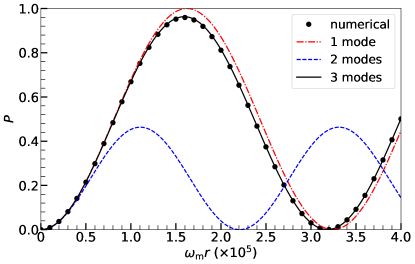
Figure 3: Same as Fig. 2 but with $\lambda_{2}/\omega_{\mathrm{m}}=0.1$ and $k_{2}/\omega_{\mathrm{m}}=10$.

In Fig. 3 we demonstrate another case with the second Fourier mode being a short-wavelength mode ($k_{2}=10\omega_{\mathrm{m}}$ and $\lambda_{2}=0.1\omega_{\mathrm{m}}$). In this case, although each of the two off-resonance Rabi modes $O_{\pm}$ is capable to suppress the Rabi transition by a large amount, the shifts of the resonance frequency due to these two modes are in opposite directions [see Eq. (39)]. As a result, the suppression of the Rabi transition is not significant in the actual system.

We note that, according to the discussion in Sec. III.1, for a given on-resonance Rabi mode (which is relevant to a physical system), Eq. (31) implies that only a finite number of off-resonance modes can satisfy the criterion in Eq. (42), although an infinite number of Rabi modes exist in the system due to the Jacobi-Anger expansion. For small perturbations where the amplitudes of all Rabi modes are much smaller than $\omega_{\mathrm{m}}$, Eq. (42) demands that the amplitude of a single off-resonant Rabi mode must be significantly larger than that of the on-resonance mode to affect the resonance. This can be true if the on-resonant Rabi mode involves a few participating Fourier modes and, therefore, has an amplitude much smaller than that of an off-resonant Rabi mode with only one participating Fourier mode. Even for an on-resonant Rabi mode with a single participating Fourier mode, the ac Stark shifts of many off-resonance, long-wavelength Rabi modes can add up and change the resonant behavior according to Eq. (43).

IV Conclusions

We have shown that the neutrino oscillation Hamiltonian with an oscillatory matter profile can be treated as a Rabi system with an infinite number of Rabi modes each with contributions from various Fourier modes of the matter profile. Neutrino flavor conversion can be greatly enhanced if a Rabi mode is almost on resonance. Although the existence of the harmonic parametric resonances have already been shown in Refs. Kneller:2012id ; Patton:2013dba , our derivation adds more intuitive understanding to this interesting phenomenon.

We have shown that the number of the Fourier modes that participate in a Rabi mode and their contribution orders cannot be too large or the amplitude of the Rabi mode becomes too small to be relevant. As a result, only a finite number of Rabi modes need to be considered for a real physical problem. We have also gone beyond the rotating wave approximation and studied the interference between Rabi modes. This interference effect is different than the suppression of the parametric resonance by certain long-wavelength Fourier modes discussed in Ref. Patton:2013dba . It is also different than the three-flavor effect discussed in Ref. Yang:2015oya . We have shown that an off-resonance Rabi mode can significantly change the parametric resonance of neutrino flavor conversion if the amplitude of the off-resonance mode is sufficiently large. We have derived an explicit criterion of whether an off-resonance Rabi mode can affect the parametric resonance. A Fourier mode in the matter fluctuation always results in (an infinite number of) pairs of Rabi modes. Each pair of these Rabi modes have the same amplitude but rotate in the opposite directions. We found that the interference effects due to a pair of such Rabi modes add up coherently if they have long wavelengths, and they tend to cancel each other if the wavelengths of the Rabi modes are short. As a result, the Fourier modes with long wavelengths are much more likely to affect the parametric resonance than the short-wavelength modes.