Variability and Jet Activity in the YSO MHO 3252 Y3 in Serpens South

Abstract

The infrared young stellar outflow source MHO 3252 Y3 in the Serpens South star-forming region was found to be variable. The available photometric data can be fitted with a double peaked light curve of 904 d period. Color variations are consistent with variable extinction with a flatter wavelength dependence than interstellar extinction, i.e., larger grains. MHO 3252 Y3 is the source of a large scale bipolar outflow, but the most recent outflow activity has produced a microjet detectable in the shock excited H₂ 1–0 S(1) line while [Fe II] emission appears confined to the immediate vicinity of the central star. The proper motion of individual shock fronts in the H₂ microjet has been measured and traces these knots back to ejection events in the past two centuries. Integral field spectroscopy with the Keck 1 adaptive optics system and the OSIRIS instrument shows velocity components near the launch region that are distinct from the microjet both in radial velocity and apparent proper motion. They match the prediction of dual wind models with a distinct low velocity disk wind component. We find evidence for the entrainment of this low velocity component into the high velocity microjet, leading to shock excited emission at intermediate velocities in an envelope around the microjet.

1 Introduction

The accretion process forming stars out of much larger molecular clouds can only proceed if the excess angular momentum of the original – usually rotating – molecular cloud material can be disposed of. This is achieved by the ejection of a fraction of the infalling material in the form of bipolar molecular outflows. The first such outflow was discovered by Snell et al. (1980) in millimeter CO emission. Faster, more collimated jets of molecular and atomic material were discovered at optical wavelengths by proper motion studies of HH objects (Herbig & Jones, 1981) and by the first imaging studies of the jets themselves by Dopita et al. (1982), Graham & Elias (1983), Mundt et al. (1983), and Mundt & Fried (1983). The region where jets are launched and then collimated is so close to the central star that observations with the highest achievable spatial resolution are required. Velocity resolved observations of the first few hundred astronomical units of a jet have been done with the Hubble Space Telescope (HST) at optical and near-infrared wavelengths, and most recently with integral field spectrographs and adaptive optics systems on ground-based large telescopes. However, only a small number of protostellar jet sources could, so far, be studied because they either must be optically detectable for HST or have an optically visible nearby tip-tilt reference star for ground-based adaptive optics work in the near infrared.

This paper does not intend to present a review of the extensive literature on protostellar outflows and jets. The reader is referred to Reipurth & Bally (2001) for a review of the older literature, and the more recent review by Frank et al. (2014) at the Protostars & Planets VI Conference.

While all the cases studied in detail show large-scale outflow, a diversity of phenomena has emerged near the driving source, probably dependent on the mass, evolutionary state, and orientation of the object. Among the jet sources studied with sufficient detail both classical jet features as well as series of bubbles have been observed. In some cases, microjets of only a few arcseconds in length can be observed that kinematically are only decades to a few centuries old and therefore offer the best opportunity for studying the conditions of their launch. Some objects actually show both a jet and bubbles in different excitation tracers. The very young outflow phase T Tauri star XZ Tau was imaged repeatedly by Krist et al. (2008) using HST and shows a series of bubbles rather than a typical jet while the immediately adjacent HL Tau shows classical jet features. A similar pattern of bubbles traced in the H₂ 1–0 S(1) line has been observed in NGC 1333 SVS13 studied by Hodapp & Chini (2014). In this outflow object a jet is observed in the high-excitation [Fe II] line, while the lower excitation H₂ 1–0 S(1) line shows the morphology of a string of bubbles. Another example of spherically expanding shock fronts, rather than jets, is the high-mass protostar in Cepheus A HW2, where Torrelles et al. (2001) observed an expanding ring of H₂O masers.

On the other hand, objects showing a well collimated microjet generally exhibit a complex velocity structure, as was reviewed in, e.g., Frank et al. (2014): A high velocity component (HVC) associated with the well collimated microjet itself, and a low velocity component that is spatially distinct, broader and best observable in mm-wave emission lines of CO. We will, in the following, refer to the latter as the broad low velocity component (BLVC). Shock-excited emission from such a BLVC is usually identified with the interaction of a low velocity disk wind with the outflow cavity. Detailed velocity studies of YSO jets often show velocity gradients in the jet from the HVC on the jet axis to an intermediate velocity component (IVC) forming an envelope around the jet. Its formation and excitation is best explained by lateral entrainment of the BLVC wind by the HVC of the jet, as discussed in detail for the case of DG Tau by White et al. (2016), even though this issue is still actively being debated.

We will frequently refer to DG Tau as a comparison case in the discussion of our object MHO 3252 Y3, and therefore introduce DG Tau in some level of detail. The DG Tau jet was first imaged by Mundt & Fried (1983) and then studied spectroscopically in forbidden emission lines at optical wavelengths by Bacciotti et al. (2002), and in [Fe II] by Pyo et al. (2003) with Subaru IRCS. A detailed study of the proper motion of the DG Tau jet knots based on VLA radio, optical, and X-ray data was presented by Rodríguez et al. (2012). They found that optical/infrared emission knots coincide with the VLA radio knots, identify one X-ray emission knot earlier seen in optical emission and present a geometric model of the DG Tau bipolar outflow.

Velocity-resolved integral field spectroscopy was presented by Agra-Amboage et al. (2011) and
Agra-Amboage et al. (2014) with the ESO/SINFONI integral field spectrograph and independently by White et al. (2014a) and White et al. (2016) using Gemini/NIFS. The microjet in DG Tau is detected in [Fe II] emission, while the H₂ 1–0 S(1) emission line shows only a BLVC. The blueshifted part of the DG Tau microjet has two velocity components in [Fe II]: A well collimated high velocity (HVC) microjet, enveloped by an intermediate velocity component (IVC). The redshifted outflow lobe of DG Tau, however, shows only the wider BLVC with a bubble-like structure traced both in the [Fe II] and H₂ 1–0 S(1) emission lines.

The DG Tau microjet is comprised of multiple emission knots, formed by internal shocks within the jet. Their spacing indicates that events leading to the formation of different velocity ejecta must occur every few years. Older determinations of the bubble spacing by Pyo et al. (2003) indicated a 5 yr period, confirmed by Rodríguez et al. (2012) while Agra-Amboage et al. (2011) claimed that the ejection period is even shorter at 2.5 yr. White et al. (2014b) discussed all available studies of the ejection interval and in the end concluded that the ejection interval is variable and subject to future studies.

Any accretion process from a rotating molecular cloud onto a protostar must solve the problem of excess angular momentum of the infalling gas. Rotation of the jet would provide a mechanism for ejecting angular momentum and for allowing most of the infalling matter to accrete onto the star. Observational confirmation that protostellar and T Tauri jets do indeed rotate has proven exceedingly difficult, however. The state of this field has recently been reviewed by Frank et al. (2014). In their paper on the ultimately unsuccessful search for rotation in the RY Tau jet, Coffey et al. (2015) noted that for a convincing detection of rotation, it should be detected near the driving star, should be consistent along the jet, should rotate consistent with the rotation of the disk, and be independently confirmed by other observers. So far, no optical/NIR jet has satisfied this strict set of criteria. Even for the best studied jet at optical and near-infrared wavelengths, DG Tau, which we introduced above, rotation studies in different emission lines and by different authors remain inconsistent.

There have been some successful detections of rotational signatures at sub-mm and mm wavelengths, using the superior velocity resolution of heterodyne radio receivers, e.g., CB 26 (Launhardt et al., 2009), DG Tau B (Zapata et al., 2015), Ori-S6 (Zapata et al., 2010), NGC 1333 IRAS 4A2 (Choi et al., 2011), and HH 797 (Pech et al., 2012), while others ascribed observed asymmetric kinematic features of jets to the effects of orbital motion, e.g. (Lee et al., 2009) and (Lee et al., 2010). A particularly convincing example of rotation in the protostellar jet HH 212 has recently been published by Lee et al. (2017) and Lee et al. (2018) using ALMA data of high spatial and spectral resolution.

The Serpens South star forming region, discovered by Gutermuth et al. (2008) is the site of multiple very young stars in their accretion and outflow phases. The most reliable distance to the Serpens complex of molecular clouds, of which Serpens S is a part, has been measured by Ortiz-León et al. (2017) to be 436.0$\pm$9.2 pc, based on VLA parallax measurements of several radio-bright YSOs in that cloud. We adopt this distance here and refer the reader to the extensive discussion in the paper by Ortiz-León et al. (2017) of different distance determination methods, older distance measurement, the spatial structure of the Serpens molecular cloud, and its association with larger structures. In the Appendix, we also briefly discuss one star near Serpens South with a Gaia (Gaia Collaboration, 2016) DR2 distance measurement and conclude that its measured distance is consistent with that determined by Ortiz-León et al. (2017).

Teixeira et al. (2012) have conducted a search for molecular hydrogen shock fronts of bipolar outflows of young stellar objects (YSO) in the Serpens South region, and have included many of them in the catalog of Molecular Hydrogen Objects (MHO) (Davis et al., 2010) . In particular, the outflow source listed as MHO 3252 Y3 by them at $\rm 18^{h}30^{m}01\fs 3~{}-2\arcdeg 10\arcmin 26\farcs 0~{}(J2000)$ has attracted our attention as a variable infrared object with substantial amplitude and a 904 d period. These observations will be described in section 2.1 and 3.1. MHO 3252 Y3 is the driving source of a short, highly collimated microjet with multiple shock fronts, as well as a more extended system of older shock fronts, traced in the shock-excited H₂ 1–0 S(1) line. As an overview of this object we show an RGB false color composite of UKIRT WFCAM $H$, S(1) line, and $K$-band images in Figure 1. The $S(1)$ line image (green) is substantially deeper than the image by Teixeira et al. (2012) and shows a well developed, though faint bow shock in the eastern outflow lobe. Proper motion measurements, discussed later in chapter 3.2, are also indicated in Figure 1.

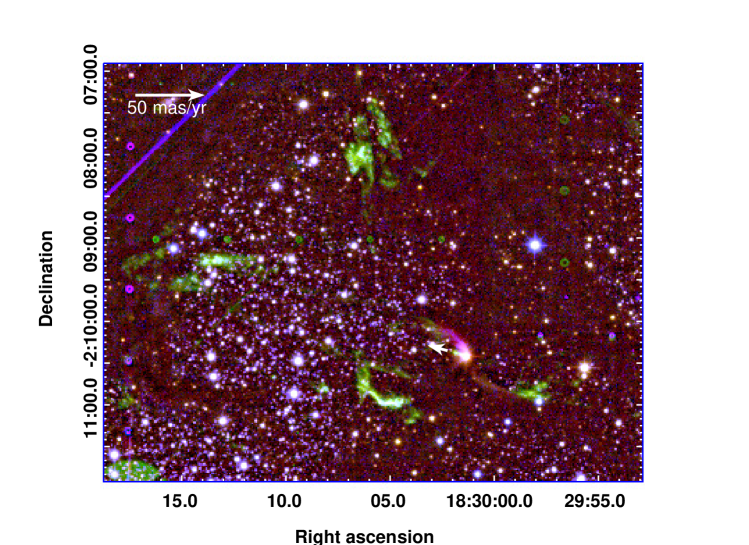
Figure 1: Three color composite of $H$-band (blue), $S(1)$ line emission (green), and $K$-band (red) UKIRT WFCAM images of the Serpens South MHO 3252 Y3 region, obtained in 2016 and 2017. Shock-excited features show up in green. MHO3252 Y3 is the source of a large-scale well developed bipolar outflow. Proper motion vectors based on the 2011 Calar Alto data of Teixeira et al. (2012) and on 2016 UKIRT data are indicated.

The small extent of the microjet of only a few arcseconds and the availability of a sufficiently bright star for tip-tilt correction make this object a suitable target for adaptive optics integral field spectroscopy with the OSIRIS instrument on Keck 1, allowing a combination of diffraction-limited spatial and medium spectral resolution. These observations will be presented in sections 2.2, 3.2, 3.3, and 3.4 and discussed in section 4.

There are only a few examples of microjets of young low mass stars that are suitable for detailed studies. Each of these examples show individual peculiarities, and a generalized picture of jet formation can only be formed by studying as many as possible of the available cases. This paper adds MHO 3252 Y3, a small, relatively low excitation microjet, to the list of well studied cases of protostellar jets.

2 Observations and Data Reduction

2.1 IRIS and UKIRT Imaging Photometry

As part of an on-going program of monitoring star-forming regions for variable objects, from 2012 on, the area of MHO 3252 Y3 was repeatedly imaged in the $K_{s}$ band (Skrutskie et al., 2006) with the IRIS 0.8m telescope (Hodapp et al., 2010) and 1024$\times$1024 2.5 $\mu$m IRIS infrared camera of the Universitätssternwarte Bochum on Cerro Armazones, Chile. This infrared camera was described in detail under its old name (QUIRC) and in its original optical configuration by Hodapp et al. (1996). For each visit of a specific region, IRIS takes 20 raw data frames on the object with an integration time of 20 s, with small dithers to get around detector defects, followed by 20 dithered data frames on a separate sky field chosen to avoid bright stars or extended nebulosity. For these sky exposures, larger dithers are used than for the object exposures to minimize the impact of any nebular emission on the computation of the sky frame.

The source MHO 3252 Y3 reaches $K_{s}\approx$ 10 in maximum brightness, which is near the bright limit for the standard 20 s exposures with IRIS used for monitoring. We therefore base the light curve of this object on the ”short” IRIS exposures. After detector reset and the first of the reads of the double correlated pair of readouts, the IRIS camera immediately reads the detector out a second time, before the rest of the 20 s nominal integration time elapses. The difference of these two frames early in the integration time is a double-correlated pair with an effective integration time of 2 s. The sensitivity of this short integration is entirely adequate even for recording the $K_{s}\approx$ 12 minimum of the MHO 3252 Y3 light curve and therefore the IRIS photometry of MHO 3252 Y3 is based on these short exposures.

The IRIS camera raw data were processed in a reduction pipeline written by R. Watermann and based on the Image Reduction and Analysis Facility (IRAF) software (Tody, 1986). The raw data were flatfielded using incandescent light differential dome flats. Sky frames are computed as the sky-background adjusted median of the sky position frames taken at some distance from the star-forming region and its extended nebular emission, and then subtracted from the object frame. The optical distortion correction was based on an as-built ZEMAX model of the optical system. After correcting the known optical distortions, the astrometric solutions of the individual images were calculated using SExtractor (Bertin & Arnouts, 1996) and SCamp (Bertin, 2005) and based on Two Micron All Sky Survey (2MASS) coordinates (Skrutskie et al., 2006). The images were then co-added using these astrometric solutions. Aperture photometry was obtained with the IRAF task PHOT with an aperture of $r=4$ pixels ($r=3\arcsec$) and calibrated against an ensemble of stars from the 2MASS catalog. These 2MASS reference stars were selected for appropriate brightness, and for being isolated from other stars and from nebular emission. The 2MASS reference stars were in the brightness range K_s = 12.5 - 14.5. For part of the monitoring period, the IRIS telescope experienced unusually large pointing errors and unstable image quality due to a mirror support problem, so that there are only 9 suitable 2MASS photometric reference stars common to all IRIS frames used here. The rms scatter of the measured magnitudes ranged from 0.03 for the brightest to 0.10 mag for the faintest reference stars.

In addition to the monitoring with IRIS, deeper images with better spatial resolution were obtained with the Wide-Field Camera (WFCAM) (Casali et al., 2007) on UKIRT in 2016 and 2017. The WFCAM filters conform to the ”MKO” standard described by Tokunaga, Simons, & Vacca (2002) and further characterized in Tokunaga & Vacca (2005). As is done in the UKIRT manuals, we will refer to the UKIRT $K$ bandpass simply as ”$K$”. The UKIRT images in the $J$, $H$ and $K$ broad bands and in the narrow S(1) line filter are substantially deeper than those of Teixeira et al. (2012) and show additional details of the shock fronts. The UKIRT WFCAM data were processed by the pipeline run by Cambridge Astronomy Survey Unit (CASU), and the delivered FITS image files were directly used for photometry. For the purpose of determining the light curve, we did not do any color correction between the IRIS K_s and the WFCAM $K$ filters, and refer the combined lightcurve bandpass simply as ”$K$”. We have also added two photometric data points from the 2 m Fraunhofer Telescope (Hopp et al., 2014) on Mt. Wendelstein in Germany, taken with the 3kk optical/infrared camera (Lang-Bardl et al., 2016). For all photometry, the same angular size ($r=3\arcsec$) of integrating aperture was used. As a side note, the $K$-band image of Teixeira et al. (2012) is saturated, so that we could not use it to extend the coverage of our light curve.

2.2 Keck OSIRIS Spectroscopy of the Microjet

MHO 3252 Y3 is sufficiently close to an optically visible star to allow tip-tilt correction with the Keck 1 Laser Guide Star Adaptive Optics (LGSAO) system. However, this tip-tilt star is at the limits of the acquisition range and near the practical limiting magnitude for guide stars, so that the performance of the LGSAO system is strongly dependent on the prevailing natural seeing. We have obtained Keck OSIRIS observations at three epochs under varied seeing conditions. Table 1 summarizes these observations and indicates the quality of the resulting data. The 2012 observations were done with the coarse 100 mas scale of OSIRIS (Larkin et al., 2006), and had the character of ”quick first look” observations. Nevertheless, the wavelength-integrated images in the H₂ 1–0 S(1) line extracted from these observations served as the first epoch data for the study of the microjet proper motion. Also, the [Fe II] emission line at 1644 nm was detected in spectra taken through the OSIRIS Hn3 filter in 2012. We have not pursued [Fe II] observations any further since this line is faint and its emission region is spatially unresolved. In 2015, some setup observations were taken with the 100 mas scale, which we in the end did not use due due to problems with the PSF delivered by the AO system. The 20 mas data from that run were of very good quality and are the basis for the detailed study of the velocity field near the launch region of the jet. In 2017, data were taken both in 100 mas and 20 mas scales. The seeing was noticeably worse than in 2015, and consequently, of the 2017 data, we are only discussing the deep data in the 100 mas scale, both for jet proper motion and radial velocity studies.

The OH-Suppression Infrared Imaging Spectrograph OSIRIS (Larkin et al., 2006) produces spectra of the pupil images formed by each of its lenslets. The spectral resolution depends on the quality of this pupil image formed by each lenslet, and therefore varies across the field of view. The median spectral resolution at the wavelength of our H₂ 1–0 S(1) line observations is $\approx$ 3500. The typical velocities found in protostellar jets are of the same order as the spectral resolution of the instrument.

The OSIRIS underwent two upgrades during this project. The grating in OSIRIS was upgraded in 2013, leading to better efficiency (Mieda et al., 2014) and the detector was upgraded in 2016 to a H2RG detector with better quantum efficiency. These changes to the instrument changed the wavelength calibration and were accounted for by updates to the data reduction pipeline. The foreoptics, and therefore the spaxel scale and the astrometric calibration, were not affected by the instrument upgrades.

Table 1: Keck OSIRIS Observations

Date	100 mas	20 mas	Grating	Detector
2012 07 30	S(1) epoch 1	no data	old	old
	[Fe II]
2015 05 30	Poor PSF	Radial Velocity	new	old
2017 08 31	S(1) epoch 2	Poor Seeing	new	new
	Radial Velocity

The OSIRIS data reduction pipeline (DRP) was used to extract the spectra of each individual lenslet that defines the spatial spaxels. The extraction parameters are calibrated with lamp spectra and stored in the form of a ”rectification matrix” that the DRP uses to produce a data cube with a nominal wavelength calibration. The remaining data analysis work was done using custom IRAF scripts. The data cubes were magnified in the spatial dimension and cleaned of cosmic ray events and other defective pixels. To have an independent verification of the wavelength solution during the observations, we used several bright OH airglow lines that were recorded in the wavelength range of the Kn2 filter used for our observations of the H₂ 1–0 S(1) line. Two bright OH airglow lines – 9-7 R1 (2.5) at 2117.6557 nm and 9-7 R1 (1.5) at 2124.9592 nm (Rousselot et al., 2000) – are located on either side of the H₂ 1–0 S(1) line. The average of those two lines is 2121.30745 nm very close to the laboratory wavelength of the S(1) line of 2121.833 nm (Bragg et al., 1982). For each of these two OH lines, we computed, for each spatial spaxel, the centroid of the OH airglow line. The average of these two centroid frames gives the wavelength calibration zero point at 2121.30745 nm, which is within the wavelength range of the blueshifted velocity components of the observed S(1) emission. We found that the wavelength calibration was dependent on the spaxel position in the field of view. To correct measured velocities for this, we computed an image of the centroids of the S(1) emission, initially calibrated in nominal DRP wavelength spaxels. Subtraction of the wavelength calibration zero point, subtraction of the difference in wavelength spaxels from that average OH wavelength to the rest wavelength of S(1), calibration of the dispersion, conversion to velocity, and subtraction of the VLSR, results in an image of the velocity field of the S(1) emission.

For the [Fe II] observations, the OH airglow line produced by the transition 5-3 R1 (2.5) at a vacuum wavelength of 1644.2155 nm Rousselot et al. (2000) served as a wavelength calibration reference and a measure of the instrumental resolution.

3 Results

3.1 $K$-band Light Curve

The raw light curve resulting from all the $K$ band observations is shown in Figure 2. It is only sparsely sampled, mainly due to constraints on the observability of the object, but also due to some technical problems with the IRIS telescope over the course of the 5 year monitoring campaign. Nevertheless, the lightcurve of MHO 3252 Y3 shows substantial changes in brightness with a first indication of a possible period of $\approx$ 2.5 years between major minima. We have used several period determination algorithms implemented in the PERANSO software written by T. Vanmunster, each of which gave similar results for the period: Dworetsky (1983): 902.32 d, Renson (1978): 906.6 d, Lafler & Kinman (1965): 901.5 d, Schwarzenberg-Czerny (1996): 904.4 d.

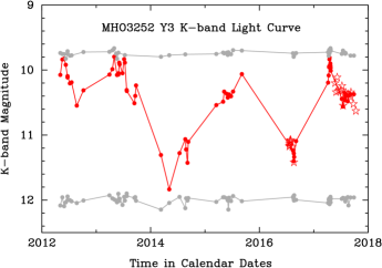
Figure 2: The light curve of MHO 3252 Y3 in the $K$ band is shown in red. The data were obtained with the IRIS telescope (filled circles) and UKIRT and the Fraunhofer Telescope (open star symbols) from 2012 - 2017. For comparison, the IRIS photometry of two apparently constant stars in the field are also shown (grey color), to demonstrate the reliability of the photometry and the typical errors involved in the IRIS telescope photometry of similarly bright stars. Two major dimming events, $\approx$2 mag deep, have occurred in 2014 and 2016 and minor dimming events have been observed in 2013 and again in 2017.

Somewhat naively taking the average and standard deviation of these period determinations with different algorithms gives P = 904 d $\pm$ 7 d (3$\sigma$). The light curve was phased using this period of 904 days and an arbitrarily chosen epoch of JD 2457857.8047 (2017 April 14) the day during the 2017 visibility period when the brightest measurement of the first flux maximum was obtained with IRIS. This phased light curve shows two maxima of nearly the same brightness, and two minima of very different depth, the first reaches down to $K\approx$ 10.5, the other down to $K\approx$ 11.8. The first maximum is characterized by a sharp increase in brightness from the previous deep minimum, while the second maximum is broader, with a slower rise from the preceding shallow minimum. The second maximum does not occur at phase 0.5, but rather earlier, at phase $\approx$ 0.45, so it is unlikely that the true period is 904/2 d = 452 d.

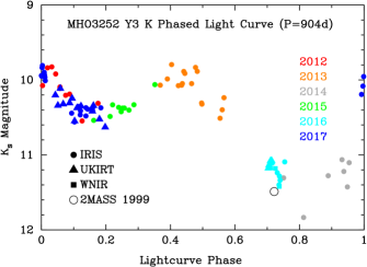
Figure 3: The light curve of MHO 3252 Y3 in the $K$ band phased with a period of 904 d. The different colors indicate the year of the respective observations. The phase is set zero at the epoch of the brightest measurement in 2017 on JD 2457857.8047 (2017 April 14).

Figure 3 shows this phased light curve with the data points identified by year via color, and by telescope via symbols. The period is roughly 2.5 yr, and therefore, any part of this light curve will only be observable every 5 yr. With the presently available data the period determination largely relies on matching the 2012 and 2017 data of the decline from the first maximum and on the partial overlap of the 2015 and 2017 data on the first shallow minimum. The 2014 and 2016 data on the deep second minimum just barely overlap. The fact that the 2MASS catalog (Skrutskie et al., 2006) magnitude of K_s=11.489, observed on 1999 April 5, i.e., 13 years before the other measurements reported here, fits well into this phased light curve gives some confidence in the validity of this period determination. The 2018 visibility period will cover the broader second maximum between phase 0.4 and 0.6 again, which was already covered in 2013. The 2019 visibility period will cover the heretofore poorly observed broad minimum and the increase back to maximum light (phases 0.8 to 1.0). It remains to be seen whether the light curve in the next two years will match the prediction of this period fit to the last 5 years of data, or whether new light curve features will emerge.

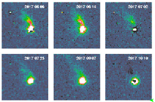
Figure 4: Difference images (30″$\times$30″) of MHO 3252 Y3 in the $K$ band obtained with UKIRT WFCAM during the 2017 observing season. The average of all images in 2017 was subtracted from each individual image, so that subtle changes in the illumination of the reflection nebula become more noticeable. Note that the S(1) line emission of the jet is not visible in these difference images since its flux is constant on the timescale of months and therefore subtracts out.

We have also analyzed the broad-band $K$ images for photometric variations of the reflection nebula associated with MHO 3252 Y3. In Figure 4, we show difference images at 6 selected epochs during the 2017 observing season where the average image of all these frames obtained in that year was subtracted from the individual images. The images are shown here in logarithmic scale in color-coded intensity, and changes in the overall brightness of the image as well as changes in the illumination of various components of the reflection nebula are clearly indicated.

3.2 Shock Front Proper Motion

The deepest UKIRT data are summarized in Figure 1, a $H$-$S(1)$-$K$ false color image. For Figure 1, the deep UKIRT S(1) data obtained between 2016 July 21 and 30 were combined with the sums of all the $H$ and $K$-band UKIRT images taken in 2017 for the photometric monitoring campaign. Molecular hydrogen 1–0 S(1) emission stands out as green features in this color composite. In particular, it is clearly seen that MHO 3252 Y3 is the source of a system of molecular hydrogen shock fronts that extends well beyond the highly collimated microjet close to the driving source. Figure 1 also shows the proper motions of S(1) shock fronts, measured from our UKIRT 2016 S(1) image and the 2011 July 16 S(1) data taken by Teixeira et al. (2012) that we downloaded from the Calar Alto Data Archive. After initially registering the two images with the IRAF tasks GEOMAP and GEOTRAN, the crosscorrelation of the two images was calculated in boxes centered on individual shock fronts using XREGISTER, and comparison crosscorrelations were done on boxes close to the emission features but only containing stars. We found the pattern of cross-correlation shifts of background stars to be non-uniform across the 2011 reference image, and therefore, we have only subtracted these cross-correlation shifts of stars locally from the shifts measured for adjacent shock features. As a result, these proper motion vectors, indicated in Figure 1, are in reference to background stars, and not to the driving source of the outflow. We could not get any reliable proper motion measurements of the eastern bow shock. The bow shock itself was too faint on the S(1) image from Teixeira et al. (2012) for a measurement. One set of brighter knots just behind the bow shock has many background stars and therefore the cross-correlation technique does not work there and we consider the proper motion vectors of these emission knots as unreliable.

We have also measured the proper motion of the microjet emanating from MHO 3252 Y3 on the OSIRIS data cubes obtained with the 100 mas spaxel scale of the instrument in 2012 and 2017. The raw data cubes were cleaned of spurious pixels produced by cosmic rays and similar noise spikes. Continuum subtracted images were produced by integrating over all wavelengths with significant H₂ 1–0 S(1) emission, and subtracting a continuum image produced by similarly integrating over adjacent continuum wavelengths. The proper motions of individual shock fronts were calculated by cross-correlation (IRAF task XREGISTER) of the 2012 and 2017 line-integrated and continuum-subtracted data within the integration boxes indicated in Figure 5. The cross-correlation shift of the continuum position of the central star was subtracted from the shifts measured for the shock fronts. The proper motion vectors in Figure 5 therefore refer to the central star. The proper motion of the brightest S(1) emission knot in the jet is also included in the wide-angle image Figure 1, as a representative proper motion value for the whole microjet.

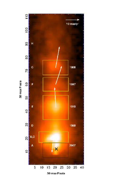
Figure 5: Keck 1 OSIRIS 100 mas/pixel data integrated over the H₂ 1–0 S(1) emission in MHO 3252 Y3. The image was rotated by 71$\fdg$5 to show the jet axis approximately vertical. MHO 3252 Y3 shows a well collimated microjet with pronounced knot structure, indicating a variable jet ejection speed. The proper motion vectors from 2012 to 2017, measured in the integration boxes outlined in yellow, are indicated by the white arrows. The proper motions are relative to the central star of MHO 3252 Y3 whose proper motion was measured in the box outlined in black. The emission knots are labeled in the same way as in Figures 6 and 7 and the approximate ejection date of each emission knot calculated from its distance and the average proper motion is indicated.

The epoch difference between the two OSIRIS 100 mas data sets from 2012 July 13 (JD 2456121.5) and 2017 August 31 (JD 2457996.5) is 1875 d = 5.133 yr For the best defined S(1) emission knot, labeled ”E” in Figures 5 and 6 we measured a proper motion of 14.784 $\rm mas~{}yr^{-1}$ or 30.56 km s^-1 tangential motion at the adopted distance of 436 pc.

The median radial velocity (see Section 3.3) of this knot was measured over the same integration box as was used for the cross-correlation for the proper motion measurements and was calculated relative to the motion of the molecular cloud in the – unproven – assumption that this is a good proxy for the motion of the central star. This measured radial velocity of the knot of -86 kms^-1 relative to the star, implies that the jet is oriented only 19$\fdg$6 inclined against the line of sight.

3.3 OSIRIS Radial Velocity Measurements

We are presenting the radial velocity information from the ”wide field” 100 mas spatial scale data in Figure 6, and in Figure 7 for the ”high resolution” 20 mas scale of OSIRIS. In both figures we have coded the radial velocity by color, and have multiplied the resulting RGB color image by the line-integrated intensity, such that a zero intensity shows as a white color and the color saturation level indicates intensity. The reason for this method of presenting the velocity data is to prevent regions of low flux from dominating the velocity diagram with high-noise pixels.

Our velocity data are presented relative to the local standard of rest velocity (VLSR) and all measured velocities are blueshifted relative to this velocity. From the ¹³CO measurements of Nakamura et al. (2017), the velocity of the Serpens S molecular cloud and of the nearby W 40 complex is 7 km s^-1 relative to VLSR and they argue that both the angular proximity and essentially identical velocity strongly suggest a physical connection of the two clouds. If we assume that the driving source of MHO 3252 Y3 has the same velocity as the surrounding molecular cloud, the jet velocities are, 7 km s^-1 more blueshifted relative to the star.

We distinguish two velocity features: 1. The well collimated, highly blueshifted velocity component that we will simply refer to as the ”jet”. The jet has an ”onion-like” nested velocity structure with a fast moving core and relatively slower envelope. 2. A spatially much wider, distinctly lower velocity component indicated in red color if Figure 7, and visible mostly in the lower velocity panels of Figure 8, that we refer to as the broad low velocity component (BLVC) in the following.

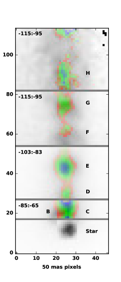
Figure 6: Velocity (coded by color) times flux (coded in color density) of MHO 3252 Y3 in H₂ 1–0 S(1) based on the OSIRIS low-resolution data that are displayed here on 50 mas pixels. The image was rotated by 71$\fdg$5 to show the jet axis approximately vertical. The velocity range displayed in the full RGB range is always 20 km^-1 VLSR, but the velocity window has been shifted in the three different regions of the figure, separated by grey lines, so that the display parameters could be individually adjusted to the different intensities and velocity ranges of the emission features, so that the velocity structure of the jet is shown optimally. A continuum image of the star has been added in grey-scale as a position reference. The highest velocities in the jet are near its center axis, while its envelope shows lower velocity due to the entrainment of the wider low velocity disk wind, the BLVC.

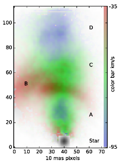
Figure 7: Velocity (coded by color) times flux (coded in color density) of MHO 3252 Y3 in H₂ 1–0 S(1) based on the high-resolution data (OSIRIS 20 mas scale) that are displayed here on 10 mas pixels. The image was rotated by 71$\fdg$5 counter-clockwise to show the jet axis approximately vertical. The velocity range is 35 $\rm km^{-1}$ - 95 $\rm km^{-1}$ as indicated by the color bar. A continuum image of the star has been added in grey-scale as a position reference. The velocity range of this figure is 3 times that of Figure 6, reflecting the large difference of the velocities of the jet (HVC) and the BLVC.

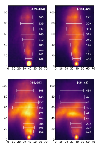
Figure 8: Four wavelength channels of the 2015 OSIRIS data in the 20 mas scale, displayed here on 10 mas pixels. These channel images were continuum subtracted, but 10% of the flux of the continuum image has been re-inserted at the position of the driving star to identify its position. Even ignoring the BLVC, several areas in the jet show asymmetric features with wavelength that create a rotational component to the velocity field. However, the velocity field is far more complicated than simply a rigid rotation of the microjet.

Individual wavelength planes of the continuum-subtracted data cube of the 2015 data in the 20 mas spaxel scale are shown in Figure 8. The spatial scale has been magnified by a factor of two, so the axes tickmarks indicate 10 mas pixels. The velocity range covered by each wavelength plane is given relative to the LSR. The motion relative to the molecular cloud, and presumably relative to the star, is 7 km s^-1 more blueshifted. The width of the jet was measured in stripes 50 mas in size in the direction of the jet axis (vertical in Figure 8) by fitting a Gaussian profile to these stripes. The symbols in Figure. 8 give the FWHM, i.e., 2.355$\times\sigma$, for compatibility with most other studies of jet width and collimation. The fastest approaching (blueshifted) components of the jet show the narrowest width, while slower approaching components are wider. This is consistent with the ”onion-layer” model of a jet where the outer layers of the jet get slowed down by turbulent interaction with a slower-moving wind component, as was discussed in the context of the DG Tau jet by Agra-Amboage et al. (2011) and White et al. (2016).

We have indicated the position of the central star by inserting the continuum image of the star at the correct position and with 10% of the original intensity. At the closest distance from the star that we could measure the FWHM, the jet already appears collimated and expands from that position monotonically with a small opening angle, until the jet passes through the broad low-velocity component. Beyond this BLVC, the FWHM measurements are more varied, possibly indicating an interaction with that low-velocity component.

3.4 Detection of [Fe II] Emission

During the initial observations in 2012, we also searched for the 1644.002 nm (Aldenius & Johansson, 2007) emission of [Fe II], but did not detect any emission from the microjet in that high-excitation line. However, faint, blueshifted [Fe II] emission was indeed detected at the position of the driving source. The spectrum in Figure 9 was extracted from a continuum-subtracted data cube in a 300 mas diameter aperture centered on the continuum source. This indicates that close to the launch region of the jet, unresolvable by our observations, Fe has been released from dust grains into the gas phase in sufficient numbers, and the higher excitation conditions exist to form the [Fe II] line emission in an otherwise very low excitation jet. Due to the low signal-to-noise ratio of this detection, we did not do any further analysis of this finding. Using the nearby 5-3 R1 (2.5) OH airglow line as a wavelength calibrator, we present the extracted spectrum in terms of velocity shift against the [Fe II] VLSR wavelength in Figure 9. The [Fe II] emission is blueshifted relative to VLSR and the Serpens S systemic velocity of 7 km s^-1 by about the same amount as the S(1) velocity components in Figure 7. The line width of the [Fe II] emission is not significantly different than that of the spectrally unresolved OH airglow line, indicating that this [Fe II] emission originates in only one velocity component.

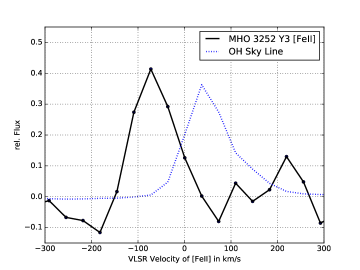
Figure 9: Spectrum of [Fe II] emission in a 300 mas diameter aperture at the position of the MHO 3252 Y3 central star. For comparison, the scaled profile of the nearby OH 5-3 R1 (2.5) OH airglow line is shown, demonstrating that the [Fe II] line is not significantly broadened.

4 Discussion

4.1 Photometric Variability

Young stellar objects are almost all measurably variable and the diversity of variability types has recently been reviewed by Hillenbrand & Findeisen (2015). The most common type of variability of young stars is the rotational modulation due to star spots on the surface, leading to short-period small-amplitude variations. MHO 3252 Y3 is clearly not of this nearly ubiquitous type of variability. Based on Spitzer Space Telescope and CoRoT (Convection, Rotation, and planetary Transit) satellite, as well as ground-based monitoring data Stauffer et al. (2015), Stauffer et al. (2014), and Cody et al. (2014) have studied young stars in their accretion phase in the NGC 2264 star-forming region. Among the stars with periodic light curves, they distinguish ”bursters” and ”dippers”, the former erupting from a quiescent brightness level, the latter dipping down from a normally bright state. A direct comparison with our observations is not straightforward, since their studies concentrated on objects with much shorter periods – a few days – than our object. More importantly, MHO 3252 Y3 does not have a well-defined ”normal” brightness level, neither at maximum nor at minimum brightness. The light curve of MHO 3252 Y3 shows that its brightness is between $\approx$ $K$=9.8 and 10.6 for most of the time, and shows one much deeper minimum down to $\approx$ $K$=11.8. Also, we note that the two maxima of the phased light curve (Figure 3) reach the same magnitude: $K$=9.8, while there is a first shallow minimum down to $K$=10.6 (phase 0.18), and a second, deeper minimum down to $\approx$ $K$=11.8 at phase 0.8. The more common state of this object is near maximum brightness and this maximum is better defined. We therefore interpret this object as a ”dipper”, and explain the variability of the central star by variations of the extinction by a thick disk structure surrounding the central star and partially obscuring the line of sight. The continuum flux from MHO 3252 Y3 probably has a substantial and possibly dominant contribution from scattered light when integrated over the aperture (3$\farcs$0) of our photometric monitoring observations. We have to expect that these variations in the extinction are individual to different scattering paths, i.e., for different parts of the reflection nebula. We have indeed observationally confirmed (Figure 4) that the changes in the reflection nebular are not uniform, but that different parts of the reflection nebula vary independently of each other.

Variability of the light distribution in young reflection nebulae has been observed for a long time, e.g., Hubble (1916) reported on the variability of the cometary reflection nebula NGC 2261, illuminated by R Mon, and discussed other earlier observations of similar objects. More recently, observations of infrared reflection nebulae, e.g., Hodapp & Bressert (2009) and Connelley et al. (2009) have shown that variability of the light distribution in such objects is rather common.

In order to increase the signal-to-noise ratio for a study of the color variations associated with the photometric variability, we have averaged all UKIRT WFCAM observations from the summer of 2016 near minimum brightness, and the first six observations from 2017, just after the maximum, in the three filters $J$,$H$, and $K$. Figure 10 shows that the amplitude of the variation measured simultaneously in $J$, $H$, and $K$ is wavelength dependent such that shorter wavelengths vary more, but that quantitatively, this wavelength dependence is flatter than that expected from varying levels of interstellar extinction in front of an object of constant color. We have plotted the expected values of the variation amplitude in $J$ and $H$, when normalized to $K$, in Figure 10 for two extinction ”laws”. The extinction law of Rieke & Lebofsky (1985) and a newer determination of the extinction law in the direction of the Galactic center (Nishiyama et al., 2009), both referring to ice-free interstellar lines of sight, predict more variation with wavelength than we observe. This is quite in line with the expectation of a flatter extinction law for the larger grains typical of protoplanetary disks.

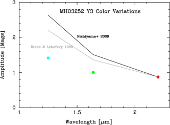
Figure 10: The amplitude of simultaneous integrated flux variations of MHO 3252 Y3 in the $J$, $H$, and $K$ filters is shown as blue, green, and red filled circles, respectively. These color variations cannot be explained by the two interstellar extinction laws shown as solid lines. Rather, the colors indicate that the absorbing dust in MHO 3252 Y3 has a flatter extinction law characteristic of a larger particle size distribution.

4.2 Morphology and Proper Motion of the Jet

The measurement of shock front proper motion in Figure 1 allows to identify the driving sources of the two outflows in this field. West of MHO 3252 Y3, the S(1) emission feature labeled MHO3252r by Teixeira et al. (2012) has a strong proper motion at P.A. $\approx$260$\arcdeg$, clearly identifying this as the western, redshifted lobe of the outflow from Y3. The eastern lobe is morphologically connected to the outflow cavity scattered light seen in continuum $K$ band by faint S(1) line emission, and the microjet is centered in this outflow cavity. This eastern lobe ends in a typical bow shock (near the left edge of Figure 1), but we could not measure any proper motions of this bow shock because the 2011 image of Teixeira et al. (2012) did not record this emission with sufficient signal to noise ratio to allow cross-correlation with our 2016 UKIRT image. The brighter emission feature behind the western bow shock labeled MHO 3252b by Teixeira et al. (2012) is superposed on several faint background stars, interfering with the cross-correlation method for the proper motion measurement. We show the resulting proper motion vectors in Figure 1, but do not believe that these measurements are valid. Despite this inconclusive proper motion measurement this feature is morphologically clearly part of the Y3 outflow and coincides with blueshifted CO emission mapped by Nakamura et al. (2011) as had already been pointed out by Teixeira et al. (2012).

We have also measured the features MHO 3251b and MHO 3255, north and south of the Y3 outflow, respectively, that coincide with blueshifted CO emission in the map of Nakamura et al. (2011) and find that their proper motions strongly suggest an origin in the Serpens S Main cluster to the north of MHO 3252 Y3, probably in the deeply embedded object P3 that Teixeira et al. (2012) had already identified as the likely driving source of the large outflow originating in the Serpens South Main cluster and moving towards the south.

In the proper motion data on the microjet in Figure 5, based on the OSIRIS 100 mas scale measurements of 2012 and 2017, the measured shift of the photocenter in the emission region ”B” is towards the star, a result that cannot be interpreted as the proper motion of a physical element of the outflow. This particular region close to the driving source shows two distinct radial velocity components, the highly blue-shifted microjet – the HVC – and a spatially wider, less blue-shifted BLVC. The wavelength-integrated image, on which the proper motion measurement is based, does not distinguish these two components, and the photocenter shift most likely is caused by changes in the relative intensity of the microjet HVC and the BLVC, rather than physical motion of either of these components. We do not have a high spatial resolution data set with the 20 mas scale of OSIRIS at the early (2012) epoch. A further investigation of motion and photometric changes of those two radial velocity components will require additional high spatial resolution data in future years.

For each well defined emission knot, we have calculated the age by dividing the distance from the star position (indicated by the X symbol) by the average proper motion of 15 $\rm mas~{}yr^{-1}$. We have listed the resulting approximate dates of the shock front ejection in Figure 5. The shock front closest to the star at a distance of only 150 mas, was therefore ejected approximately in 2007, i.e., before our monitoring campaign started. Therefore, if the ejection of this latest knot was associated with a photometric outburst, it happened just before the discovery of this object and was not recorded. Photometric outburst associated with modulations of the outflow speed should repeat themselves about every 50 - 60 years, much longer than the photometric periodicity found here.

The microjet S(1) emission observed in the UKIRT image extends for about 9″, much beyond the coverage of our OSIRIS 100 mas observations shown in Figure 6. If we assume that the microjet as a whole has the typical proper motion of those knots that we have measured, 15 mas yr^-1, its kinematic age is 600 yr.

4.3 Nested Velocity Structure in the Microjet

The MHO 3252 Y3 microjet is oriented only 19$\fdg$6 inclined against the line of sight and the radial velocity measurements are therefore very sensitive to the differential velocities within the jet. The approaching microjet has the highest blueshifted velocities in Figure 6, and therefore is shown in blue color. Intermediate velocities are shown in green. Of all the blueshifted velocity components, the relatively lowest velocity is shown in reddish color. The highest velocity blueshifted emission has the narrowest spatial width, as indicated by the blue color in Figures 6 and 7, and by the FWHM of different velocity channels in Figure 8. We identify this highest velocity component with the center of the microjet where the material had the least turbulent interaction with surrounding slower wind components, and therefore maintains the highest velocity. The highest blueshifted velocity regions in the microjet are, however, surrounded by faint emission of lower velocity, shown as a faint reddish halo around it. Alternatively, Figure 8 shows that the lower velocity channels show a wider FWHM.

We interpret this nested velocity structure surrounding the microjet as an envelope of lower velocity material, most likely the result of interaction of the microjet with a lower velocity disk wind. This velocity structure is also visible at the base of the jet in the high spatial resolution data of Figure 7, where the center of knot A shows blue color, surrounded by an envelope of slower material, shown in green, with a faint halo of low velocity material indicated in red.

Finally, the broad, relatively low velocity component (BLVC) that stands out in the proper motion study as having an apparent reversed motion is also morphologically and kinematically distinct in Figures 7 and 8. We will discuss this feature in subsection 4.5.

As already outlined in the Introduction, we are comparing our results on MHO 3252 Y3 to those on DG Tau. DG Tau is a T Tauri star in the transition phase from Class I to Class II (Pyo et al., 2003) (White & Hillenbrand, 2004), without a detected CO outflow and a faster, higher excitation microjet primarily detected in [Fe II] (White et al., 2014a) and with H₂ emission only detected directly near the collimating disk cavity. DG Tau is therefore probably less embedded and more evolved than MHO 3252 Y3.

Our findings for the MHO 3252 Y3 microjet are very similar to those for the well studied DG Tau microjet, where evidence for similar lateral entrainment was discussed by Pyo et al. (2003) and White et al. (2014a). The main difference is that the DG Tau microjet is primarily detected in the higher excitation [Fe II] line at 1644 nm while the MHO 3252 Y3 microjet is only detected in the lower excitation H₂ 1–0 S(1) line.

The formation of an intermediate velocity, shock excited layer at the interface between the high velocity microjet and the low velocity disk wind is otherwise identical to the velocity structure discussed and theoretically modeled by White et al. (2016) for DG Tau (specially their Figure 1). The salient point in their model is that protostellar microjets have an ”onion-like” velocity structure where the highly collimated fast jet turbulently entrains material from the low velocity disk wind component, forming a turbulent mixing layer of intermediate velocity that is shock-excited. It has been argued by White et al. (2016) that this mechanism, usually referred to as lateral entrainment in distinction to the frontal entrainment happening in leading bow shocks, does indeed operate even for very fast jets such as that in DG Tau when the effect of magnetic fields is accounted for. The same nested velocity structure has been found in almost all jets studied in sufficient detail, as reviewed by Frank et al. (2014).

4.4 Jet Collimation

In Figure 8 we show four individual velocity channel images of the high spatial resolution (OSIRIS 20 mas scale) data and indicate the measured FWHM of the microjet emission measured in 5 pixel high stripes. Due to its orientation towards the observer, the MHO 3252 Y3 microjet is not well suited for a study of its collimation. Therefore, our high spatial resolution velocity map in Figure 7 and the individual velocity channels in Figure 8 only show that the microjet is essentially collimated at the closest position to the star that we could get a FWHM measurement for, 70 mas from the central star, and from there only expands with a narrow expansion angle.

At the distance of MHO 3252 Y3, 70 mas distance before full collimation corresponds to a projected distance of 30.5 au from the star. The perspective shortening of the jet due to its angle of only 19$\fdg$6 against the line of sight leads to a shortening by a factor of $\approx$ 2.8. Applying this de-projection, the jet appears collimated 85 au along its axis from the star. At that position, the measured FWHM in the -104 to -69 kms^-1 velocity range is 143 mas or 62 au wide.

Model for the collimation of jet have been presented by Garcia et al. (2001) and Cabrit et al. (2007) have presented radio interferometric results on the HH 212 jet and compared those to older results on the collimation of Class II jets by Claussen et al. (1998), Dougados et al. (2000), and Woitas et al. (2002). Our results are broadly consistent with those earlier results. The MHO 3252 Y3 microjet must be essentially collimated about 85 au from the central star along the axis, at which point it is already 62 au wide. Due to larger distance of MHO 3252 Y3 and orientation towards the observer, our data cannot resolve the collimation region itself.

4.5 The Broad Low Velocity Component (BLVC)

While essentially all the S(1) line emission of the MHO 3252 Y3 microjet is blueshifted we have two components of distinct velocity, spatial extent, morphology, and proper motion. The BLVC has less than half of the radial velocity of the fastest components of the well collimated microjet. If we assume for the moment that the BLVC was generated in an eruptive event, any element of the better collimated microjet component with about double the velocity that was ejected at the same time would have had time to travel just about to the top of the field of view of the 2016 OSIRIS 20 mas observations shown in Figures 7 and 8. However, no unusual features are visible in the jet at that location. We conclude that the BLVC can only be the product of a disk instability event if this event does not at the same time affect the generation of the HVC microjet.

We again compare our results to the similar, but better studied case of the YSO jet in DG Tau. A stationary shock at the basis of DG Tau jet has been observed in [Fe II] by White et al. (2014a) and interpreted as a ”recollimation” shock from interaction of the outflowing material with the outflow cavity that collimates the outflow into a narrow jet. Observations of the emission of H₂ S(1) in DG Tau by Agra-Amboage et al. (2014) show emission over a circular area of $\approx$500 mas diameter at the basis of that jet. They presented four different models to explain a spatially broad, low velocity S(1) emission region at the base of the DG Tau jet. Considering the closer distance of DG Tau, this is about 1/3 the linear size of the low-velocity S(1) emission region in MHO 3252 Y3. Moreover, the MHO 3252 Y3 BLVC has the shape of two overlapping arcs, not a circular shape as in DG Tau. The BLVC in the MHO 3252 Y3 outflow is seen $\approx$ 450 mas from the star, a projected distance of $\approx$200 au, and a de-projected distance of over 560 au, which is much farther in linear distance than the low velocity features in the DG Tau microjet.

A possible, though speculative, explanation for this wide low velocity feature is a particularly strong internal shock within the jet that led to sideways splattering of jet material that subsequently interacts with the surrounding slower disk wind or even ambient molecular material. In their detailed study of several optically visible jets, including HH1-2 and HH 46-47, Hartigan et al. (2011) have found numerous cases of knots changing brightness, and also cases of knots and shock fronts expanding over the course of 13 years. In the outflow emanating from the binary T Tauri star system XZ Tau, Krist et al. (2008) have found a string of knots forming a jet, surrounded by a series of bubbles that interact with each other to form a broader envelope around this central jet. Similarly, in the outflow of the Class I embedded object NGC 1333 SVS13, Hodapp & Chini (2014) found a high-excitation jet, traced in [Fe II] emission surrounded by wider, lower excitation shock fronts traced in the H₂ 1–0 S(1) line, the youngest of which appear to be near spherical expanding bubbles. The jet and bubbles in NGC 1333 SVS13 were numerically modeled by Gardner et al. (2016) as an expanding bubble formed by an explosion near the star and carried away by the wind emanating from that star or a disk around it.

However, in the ”splash” scenario, we would not only expect material to be splashing away from the observer, and therefore having less blueshift, but also some material moving in the plane of the sky, at the same radial velocity as the jet, and some even moving faster towards the observer. We do not observe any emission that is more blueshifted than the core of the jet, making it difficult to explain the BLVC without resorting to the ad hoc assumption that the splash was not axisymmetric around the jet. For this reason, we do not consider this a viable explanation for the BLVC.

Machida et al. (2008) trace the evolution of the density structure, the embedded magnetic field, and the resulting magneto-centrifugal forces from the original conditions of a small (1 M_☉) molecular cloud through its collapse and to the protostellar phase with a resistive 3D MHD model and later refined the models in Machida (2014) by running the model longer to cover the full evolution of the protostellar jet. The salient feature of their models is the formation of both a low-velocity, wide-angle outflow component at densities of $\approx 1^{11}cm^{-3}$ that they identify with the source of outflows seen in $CO$ lines emission, and a much narrower, higher velocity jet component formed at protostellar densities of $\rm 5\times 10^{18}cm^{-3}$ and detected at optical and near-infrared wavelengths in shock-excited line emission. They conclude that the low velocity flow contains a large fraction of the infalling gas mass and certainly most of the total mass of the re-ejected outflowing material, as well as most of the angular momentum.

This model bears some resemblance to the two components (jet and BLVC) in our data that are distinct in spatial location and in velocity. The BLVC component of the S(1) emission can be identified with shocks of the low-velocity outflow component against the possibly still infalling envelope feeding the accretion onto MHO 3252 Y3. The cross-correlation of the integrated line intensity that was used to measure the proper motions of the jet knots shows this shock front moving back towards the star. This is likely caused by changes in brightness of the low velocity shock, and the superposition with knots in the jet that in combination appear as a backwards motion in the cross-correlation box. We do not take this ”proper motion” vector at face value, but rather as an indication that this shock is indeed not part of the jet.

We are left with two possible explanations for the low velocity wider component: 1. This could be a slow moving shock front generated by an eruptive event in the disk that affected only or mostly the slow moving disk wind, but not the faster jet that is probably generated closer to the star, or 2. The low velocity feature could be a stationary shock of the slow moving disk wind with a stationary object, possibly the wide outflow cavity responsible for the ultimate collimation of the slow wind into a molecular outflow.

Further proper motion studies of the MHO 3252 Y3 microjet at the highest available angular resolution will be able to determine whether the BLVC is a stationary shock or moving in the same direction as the microjet with about half its speed.

4.6 Rotation

The BLVC, labelled ”B” in Figures 6 and 7 has a lower radial velocity than the microjet, whose individual knots are labelled ”A, C, D …” in those figures. The displacement of the BLVC relative to the jet axis establishes an asymmetry in the velocity field. However, we do not interpret this fairly large asymmetry of the BLVC relative to the jet axis as evidence for systemic rotation and angular momentum transport in the BLVC, but rather ascribe it to the randomness of the shock interaction of the BLVC with the outflow cavity and the ambient cloud that has, apparently, led to more shock excitation on one side of the BLVC than on the other.

It is plausible that rotation of the microjet itself might be best observed very close to the central star, before turbulent interaction leads to a more complicated velocity field. We do indeed observe slight asymmetries in the collimation region very close to the MHO 3252 Y3 microjet in Fig. 7, immediately above the inserted continuum image of the star. However, this regions very close to the central star is also most affected by noise from the subtraction of the continuum emission, and minor apparent asymmetries at the jet base should therefore not be over-interpreted.

We conclude that we could not convincingly detect any rotation of the microjet in MHO 3252 Y3. This is not surprising and should not lead to generalized conclusions about microjet rotation since our proper motion and radial velocity measurement indicate that the MHO 3252 Y3 microjet is pointing strongly towards the observer and the radial velocity effect of jet rotation is perspectively reduced. Consequently, this object is not well suited for a detection of microjet rotation, even if such such rotation existed.

5 CONCLUSIONS

We have presented photometric data on the variability of the outflow and microjet source MHO 3252 Y3 and have found that a complex double-minima light curve with a period of 904 d can explain the existing observations. This phased light curve predicts that the next deep minimum will be observable in 2019. We have studied the proper motion of H₂ S(1) emission knots in the microjet and large-scale outflow of MHO 3252 Y3 and distinguish emission knots physically associated with the MHO 3252 Y3 microjet from other S(1) emission knots originating from different outflow sources. Together with radial velocity measurements, the proper motion of the microjet indicates that this jet is mostly pointed towards the observer and is only inclined by 19$\fdg$6 from the line of sight. Detailed velocity resolved integral field spectroscopy of the microjet and its launch region reveals a complex velocity field. One component, the BLVC, is much less blueshifted than the rest of the microjet, is spatially much more broadly distributed, is offset from the microjet axis, and shows an apparent proper motion essentially opposite to that of the microjet emission knots. We tentatively interpret this component as either the result of an eruptive event in the disk that mostly affected the slow wind component, but not the jet, or as the interaction of the outer layers of the slow outflow wind with the walls of the outflow cavity. The microjet itself is well collimated. Its velocity structure indicates that the outflow velocity is highest on the center axis of the microjet, and decreases outward from there due to turbulent entrainment of the slower wide wind component. No rotational velocity component in the microjet itself was observed. The microjet must be collimated within the first 85 au along its axis into a narrow opening angle. Our observations could not spatially resolve the collimation region.

Appendix A A Gaia DR2 Distance to Serpens South

The distance to W40 was precisely measured by Ortiz-León et al. (2017) to be 436.0$\pm$9.2 pc, and a plausible line of arguments leads to the adoption of this distance as the best value for Serpens South. A new and independent estimate for the distance to Serpens South is possible based on the recently released Gaia (Gaia Collaboration, 2016) DR2 catalog. This catalog contains the best available parallax measurements for all moderately bright, optically visible stars.

The Serpens South molecular cloud is essentially an opaque screen at optical wavelength and this is the reason why the Serpens South cluster had not been noticed until its discovery in the infrared by Gutermuth 2008 based on Spitzer Space Telescope data. In the direction of the Serpens South star forming region the Gaia catalog, measured at optical wavelengths, contains almost exclusively foreground stars in front of the molecluar cloud. The embedded YSO MHO3252 Y3 is a single, isolated object in the southern region of the Serpens South molecular filament. It is undetectable at the optical wavelengths where Gaia operates. One star seen near the perimeter of the heavily obscured Serpens South cluster has sufficiently low extinction to just become detectable to Gaia and this star provides a useful additional constraint on the distance to MHO3252 Y3. This star is listed as Gaia source 4270246258814194304, Pan-STARRS PSO J183007.854-020231.657, and 2MASS J18300785-0202318.‘ The star is not detected on the DSS B photographic plates. It is only weakly detected in Pan-STARRS g band and not listed in the catalog at this wavelength. The fixed aperture photometry AB magnitudes in the other Pan-STARRS bands are r = 21.328, i=17.934, z=15.701, y=14.080. The 2MASS magnitudes, converted to AB magnitudes for consistencey are J_AB=11.447, H_AB=9.631, K_sAB=9.033.

A detailed discussion of the extinction and the intrinsic spectrum of this star is beyond the scope of this discussion of its distance. Suffice it to say that the steep optical spectrum clearly shows that the star lies behind a screen of substantial extinction, which we assume is the Serpens South molecular cloud. The star could be embedded in the molecular cloud or lie behind it, so its distance measured by Gaia establishes an upper limit for the distance of that molecular cloud.

While this star is quite bright at short and mid-infrared wavelength, it does not show a long wavelenth excess and therefore was not listed as a Class 0, I, or II YSO by Gutermuth 2008. A search of the Chandra database showed that this star has not been detected at X-ray energies and it is not listed as a YSO in the X-ray selected list of (Winston et al., 2018). The star is not associated with reflection nebulosity on deep UKIRT images, unlike many other of the YSOs in the Serpens South cluster. The projected position of the star is near the periphery of the Serpens South cluster. It position makes a physical connection with the cluster plausible, but does not prove it. We do not have any positive confirmation that the star is a member of the Serpens south cluster or otherwise embedded in that molecular cloud. The Gaia DR2 distance to this star is 451 $\pm$ 79 pc When interpreted as an upper limit for the distance of the Serpens South cluster, this measurement is consistent with the Ortiz-Leon value for the distance to W40 and the assumption that Serpens South is at that same distance.

References

- Agra-Amboage et al. (2014) Agra-Amboage, V., Cabrit, S., Dougados, C., et al. 2014, A&A, 564, A11
- Agra-Amboage et al. (2011) Agra-Amboage, V., Dougados, C., Cabrit, S., & Reunanen, J. 2011, A&A, 532, A59
- Aldenius & Johansson (2007) Aldenius, M. & Johansson, S. 2007, A&A, 467, 753
- Bacciotti et al. (2002) Bacciotti, F., Ray, T. P., Mundt, R., Eislöffel, J., & Solf, J. 2002, ApJ, 576, 222
- Bertin & Arnouts (1996) Bertin, E. & Arnouts, S. 1996, A&AS, 117, 393
- Bertin (2005) Bertin, E. 2005, in Astronomical Data Analysis Software and Systems XV, ASP Conference Series, Vol. 351, eds. Gabriel, C., Arviset, C, Ponz, D., & Solano, E., 112
- Bragg et al. (1982) Bragg, S. L., Brault, J. W., & Smith, W. H. 1982, ApJ, 263, 999
- Cabrit et al. (2007) Cabrit, S., Codella, C., Gueth, F., et al. 2007, A&A, 468, L29
- Casali et al. (2007) Casali, M., Adamson, A., Alves de Oliveira, C. et al. 2007, A&A, 467, 777
- Chambers et al. (2016) Chambers, K. C., Magnier, E. A., Metcalfe, N. et al. 2016, arXiv:1612.05560, astro-PH:IM
- Claussen et al. (1998) Claussen, M. J., Marvel, K. B., Wootten, A., & Wilking, B. A. 1998, ApJ, 507, L79
- Choi et al. (2011) Choi, M., Kang, M., & Tatematsu, K. 2011, ApJ, 728, L34
- Cody et al. (2014) Cody, A. M., Stauffer, J., Baglin, A., et al. 2014, AJ, 147, 82
- Coffey et al. (2015) Coffey, D., Dougados, C., Cabrit, S., Pety, J., & Bacciotti, F. 2015, ApJ, 804, 2
- Connelley et al. (2009) Connelley, M. S., Hodapp, K. W., & Fuller, G. A. 2009, AJ, 137, 3494
- Davis et al. (2010) Davis, C. J., Gell, R., Khanzadyan, T., Smith, M. D., & Jenness, T. 2010, A&A, 511, A24
- Dopita et al. (1982) Dopita, M. A., Schwartz, R. D., & Evans, I. 1982, ApJ, 263, L73
- Dougados et al. (2000) Dougados, C., Cabrit, S., Lavalley, C., & Ménard, F. 2000, A&A, 357, L61
- Dworetsky (1983) Dworetsky, M. M. 1983, MNRAS, 203, 917
- Ferraz-Mello (1981) Ferraz-Mello, S. 1981, AJ, 86, 619
- Findeisen et al. (2013) Findeisen, K., Hillenbrand, L., Ofek, E., et al. 2013, ApJ, 768, 93
- Frank et al. (2014) Frank, A., Ray, T. P., Cabrit, S., et al. 2014, Protostars and Planets VI, 451
- Gaia Collaboration (2016) Gaia Collaboration, Prusti, T., de Bruijne, J. H. J., et al. 2016, A&A, 595, A1
- Garcia et al. (2001) Garcia, P. J. V., Cabrit, S., Ferreira, J., & Binette, L. 2001, A&A, 377, 609
- Gardner et al. (2016) Gardner, C. L., Jones, J. R., & Hodapp, K. W. 2016, ApJ, 830, 113
- Graham & Elias (1983) Graham, J. A., & Elias, J. H. 1983, ApJ, 272, 615
- Gutermuth et al. (2008) Gutermuth, R. A., Bourke, T. L., Allen, L. E., et al. 2008, ApJ, 673, L151
- Hartigan et al. (2011) Hartigan, P., Frank, A., Foster, J. M., et al. 2011, ApJ, 736, 29
- Herbig & Jones (1981) Herbig, G. H., & Jones, B. F. 1981, AJ, 86, 1232
- Hillenbrand & Findeisen (2015) Hillenbrand, L. A., & Findeisen, K. P. 2015, ApJ, 808, 68
- Hodapp et al. (1996) Hodapp, K.-W., Hora, J. L., Hall, D. N. B., et al. 1996, New A, 1, 177
- Hodapp & Bressert (2009) Hodapp, K. W., & Bressert, E. 2009, AJ, 137, 3501
- Hodapp & Chini (2014) Hodapp, K. W., & Chini, R. 2014, ApJ, 794, 169
- Hodapp et al. (2010) Hodapp, K. W., Chini, R., Reipurth, B., Murphy, M., Lemke, R., Watermann, R., Jacobson, S., Bischoff, K., Chonis, T., Dement, K., Terrien, R., & Provence, S. 2010, Proc. SPIE 7735-45.
- Hopp et al. (2014) Hopp, U., Bender, R., Grupp, F., et al. 2014, Proc. SPIE, 9145, 91452D
- Hubble (1916) Hubble, E. P. 1916, ApJ, 44,
- Krist et al. (2008) Krist, J. E., Stapelfeldt, K. R., Hester, J. J., Healy, K., Dwyer, S. J., & Gardner, C. L. 2008, AJ, 136, 1980
- Lafler & Kinman (1965) Lafler, J., & Kinman, T. D. 1965, ApJS, 11, 216
- Lang-Bardl et al. (2016) Lang-Bardl, F., Bender, R., Goessl, C., et al. 2016, SPIE 9908, 44
- Larkin et al. (2006) Larkin, J., Barczys, M., Krabbe, A., et al. 2006, Proc. SPIE, 6269, 62691A
- Launhardt et al. (2009) Launhardt, R., Pavlyuchenkov, Y., Gueth, F., et al. 2009, A&A, 494, 147
- Lee et al. (2010) Lee, C.-F., Hasegawa, T. I., Hirano, N., et al. 2010, ApJ, 713, 731
- Lee et al. (2009) Lee, C.-F., Hirano, N., Palau, A., et al. 2009, ApJ, 699, 1584
- Lee et al. (2017) Lee, C.-F., Ho, P. T. P., Li, Z.-Y., et al. 2017, Nature Astronomy, 1, 0152
- Lee et al. (2018) Lee, C.-F., Li, Z.-Y., Codella, C., et al. 2018, ApJ, 856, 14
- Machida et al. (2008) Machida, M. N., Inutsuka, S.-i., & Matsumoto, T. 2008, ApJ, 676, 1088-1108
- Machida (2014) Machida, M. N. 2014, ApJ, 796, L17
- Mieda et al. (2014) Mieda, E., Wright, S. A., Larkin, J. E., et al. 2014, PASP, 126, 250
- Movsessian et al. (2007) Movsessian, T. A., Magakian, T. Y., Bally, J., et al. 2007, A&A, 470, 605
- Mundt & Fried (1983) Mundt, R., & Fried, J. W. 1983, ApJ, 274, L83
- Mundt et al. (1983) Mundt, R., Stocke, J., & Stockman, H. S. 1983, ApJ, 265, L71
- Nakamura et al. (2017) Nakamura, F., Dobashi, K., Shimoikura, T., et al. 2017, ApJ, 837, 154
- Nakamura et al. (2011) Nakamura, F., Sugitani, K., Shimajiri, Y., et al. 2011, ApJ, 737, 56
- Nishiyama et al. (2009) Nishiyama, S., Tamura, M., Hatano, H., et al. 2009, ApJ, 696, 1407
- Ortiz-León et al. (2017) Ortiz-León, G. N., Dzib, S. A., Kounkel, M. A., et al. 2017, ApJ, 834, 143
- Pech et al. (2012) Pech, G., Zapata, L. A., Loinard, L., & Rodríguez, L. F. 2012, ApJ, 751, 78
- Pyo et al. (2003) Pyo, T.-S., Kobayashi, N., Hayashi, M., et al. 2003, ApJ, 590, 340
- Reipurth & Bally (2001) Reipurth, B., & Bally, J. 2001, ARA&A, 39, 403
- Renson (1978) Renson, P. 1978, A&A, 63, 125
- Rieke & Lebofsky (1985) Rieke, G. H., & Lebofsky, M. J. 1985, ApJ, 288, 618
- Rodríguez et al. (2012) Rodríguez, L. F., González, R. F., Raga, A. C., et al. 2012, A&A, 537, A123
- Rousselot et al. (2000) Rousselot, P., Lidman, D., Cuby, et al. 2000, A&A, 354, 1134
- Skrutskie et al. (2006) Skrutskie, M. F., Cutri, R. M., Stiening, et al. 2006, AJ, 131, 1163
- Snell et al. (1980) Snell, R. L., Loren, R. B., & Plambeck, R. L. 1980, ApJ, 239, L17
- Stauffer et al. (2014) Stauffer, J., Cody, A. M., Baglin, A., et al. 2014, AJ, 147, 83
- Stauffer et al. (2015) Stauffer, J., Cody, A. M., McGinnis, P., et al. 2015, AJ, 149, 130
- Stauffer et al. (2016) Stauffer, J., Cody, A. M., Rebull, L., et al. 2016, AJ, 151, 60
- Stellingwerf (1978) Stellingwerf, R. F. 1978, ApJ, 224, 953
- Schwarzenberg-Czerny (1996) Schwarzenberg-Czerny, A. 1996, ApJ, 460, L107
-