Visual Display and Retrieval of Music Information

Abstract

This paper describes computational methods for the visual display and analysis of music information. We provide a concise description of software, music descriptors and data visualization techniques commonly used in music information retrieval. Finally, we provide use cases where the described software, descriptors and visualizations are showcased.

1 Introduction

In the 21st century, the most common methodologies for music analysis are the visual study of the musical score and the aural and perceptual investigation of recordings[1]. In analysis courses, analysts are usually interested in creating a holistic description of a piece of music by analysing relationships and patterns, local and global, among descriptors notated on the score or perceived through listening.

Another less common but extremelly powerful methodology for music analysis is computer aided music analysis [10], also known as computational musicology or music information retrieval (MIR). This methodology is very important for companies like Spotify, Pandora[18] and Gracenote [13] who rely on algorithms and machine learning to extract information from music and listener behavior. Among musicians, computer aided music analysis and composition has been increasing, specially amid composers; among musicologists, Computational musicology is less common, perhaps due to the lack of related courses and the costs of learning a programming language and data analysis.

Information retrieval with computational means has played an important role in helping us learn about and advance our understanding of music and many other things [20]. For example, it empowers the analysis of hundreds of thousands of musical compositions with the speed of a mouse click and at the cost of few GPU cycles! It enables types of interesting analysis whose execution would be cumbersome for humans, such as understanding the distribution of events in a piece, comparing multiple performances of the same piece and understanding relationships between timbres, to cite a few. Similarly to other fields, it also empowers analysis without a precedent in history that can potentially lead to new discoveries! Last and equally important, computational musicology allows for the quantification of the musical analysis, allowing for more systematic and less subjective conclusions.

Interestingly, a recent study[7] provides evidence of the importance of data visualization in music and shows that, in the context of crowdsourcing music annotations, "more complex audio scenes result in lower annotator agreement, and spectrogram visualizations are superior in producing higher quality annotations at lower cost of time and human labor."

2 Information Retrieval

This section gives a brief description of music information retrieval in the form of pitch and timbre descriptors. It focuses on descriptors that are not easily, if possible at all, manually extracted from musical scores, audio recordings and symbolic music, e.g MIDI files or OSC. We forward the reader to [24, 17] for a survey of MIR systems and commonly used audio descriptions.

2.1 Timbre

Computing power can be used to project an audio signal from a time domain representation, e. g. amplitude over time, to a frequency domain representation, e. g. magnitude of frequency bin over time. There are many such projections and in the field of music information retrieval commonly used projections for timbre are the Spectrogram, computed with the Short Time Fourier Transform (STFT)[2], and the Mel-Frequency Cepstral Coefficients (MFCC)[14]. When computing such frequency domain representations, the time domain signal is usually divided into overlapping analysis windows. For each analysis window, the Spectrogram, as shown in Figure 1, provides the magnitude of the frequency bins.

Mel-Frequency Cepstral Coefficients (MFCC), shown in Figure 2 are probably the the most used descriptors in Automatic Speech Recognition (ASR) [11]. The MFCC arguably mimics some parts of human speech production and speech perception, specially the logarithmic perception of loudness and pitch in the human auditory system.

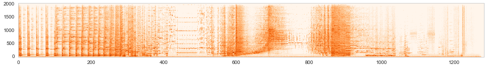
Figure 1: Beat-aligned Power Spectrogram extracted from a recording of Gerard Grisey’s Partiels. Vertical axis maps to frequency bin in hz, horizontal axis maps to time.

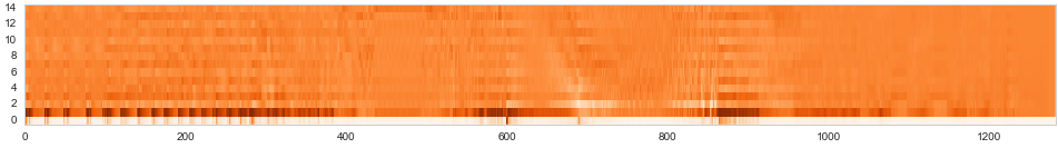
Figure 2: Beat-aligned MFCC extracted from a recording of Gerard Grisey’s Partiels. Vertical axis maps to the mel-frequency cepstral coefficient, horizontal axis maps to time.

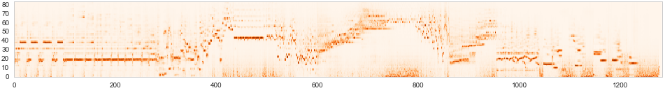
Figure 3: Beat-Aligned CQT extracted from a recording of Grisey’s Partiel. Vertical axis maps to notes, horizontal axis maps to time.

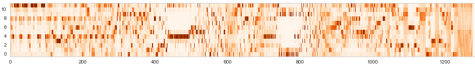
Figure 4: Beat-aligned Chromagram extracted from a recording of Grisey’s Partiel. Vertical axis maps to pitch classes, 0 is C, horizontal axis maps to time.

2.2 Pitch

There are two pitch based features that are commonly used in MIR, being the Constant Q Transform (CQT) and the Chroma. The CQT and the Spectrogram are closely related, in which they are both a bank of filters that measure the amount of energy on each frequency bin over time. In contrast to the Spectrogram, the CQT is usually interpreted as a Piano Roll given its geometrically spaced frequencies that, informally speaking, resemble the equal-tempered system and can be mapped to specific notes, e. g. the notes on a piano.

The Chroma is also referred to as pitch class profile. It is closely related to the CQT [4] in which it measures the energy of specific pitches but disregards their octave, that is, Chroma measures the amount of energy on each pitch class. Chromagrams such as the one in Figure 4, display a sequence Chroma, also known as Chromagram.

3 Information Visualization

In this section we provide an overview of visualization techniques that are commonly used in data analysis and that can facilitate the understanding of musical data. We forward the interested reader to Edward Tufte’s book [23].

3.1 Sets

In mathematics, the term set refers to a finite or infinite collection of objects in which order is not relevant and existance of an item in the set is more important than its exact count. Sets are visualized using Venn diagrams that describe the composition of each set and possible relationships. Basic set operations include union, intersection, complement and difference. Musical set theory has been considerably used in music composition [8], including computer-aided composition, and pitch analysis. The following diagram shows the pitch classes of the C major, orange, and C minor, blue, scale.

3.2 Distributions and Histograms

Similar to sets, distributions refers to a finite or infinite collection of objects in which order is not relevant. Unlike sets, distributions display the quantity of each item or numerical range, which can be represented as absolute quantity or scaled to represent the frequency of each item or numerical range. Bar graphs, pie charts, density plots, box plots are data visualizations commonly used by scientists to analyze the occurence of discrete and continuous objects.

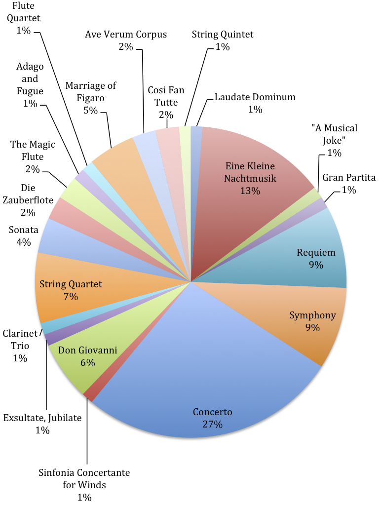
Figure 5: Pie Chart describing the usage in movies of Naxos recording of Mozart’s music.

The pie chart is a useful static visualization of proportions between data items where the area of each item is dependent on the area of other items and the total area must sum to the total area of the shape in which the data is displayed. In Figure 5 we provide one example found in a music blog that was the outcome of a class project [21].

For dynamic visualization, pie charts become cumbersome because the location and area of each item is dependent on the other items. A better tool for such cases is the bar graph, where the location of each item is fixed and their proportions is perceived by comparing the heights of each bar. Figure 6 shows an example of a pitch class histogram, represented as a bar graph, extracted using the software Music 21[9] from a MIDI rendering of Birthday by The Beatles.

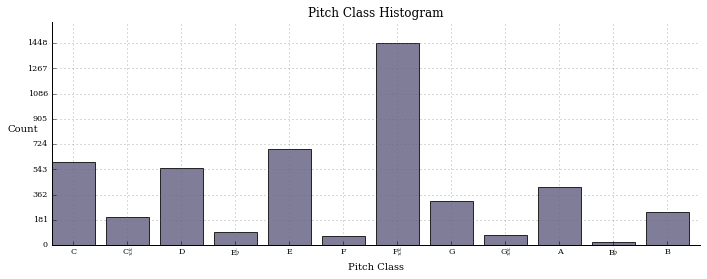
Figure 6: Histogram of Pitch Classes extracted from The Beatle’s Birthday song. Note how the most frequent notes relate to D mixolidian.

Boxplots are useful to visualize the distribution of quantities, specially quartiles, and to visualize quantities that deviate from the average quantity by some value. Box plots provide information about the spread and skewness of the data being analyzed. Multiple box plots side-by-side can facilitate the comparisson of multiple distributions, as shown in Figure 7 from [22].

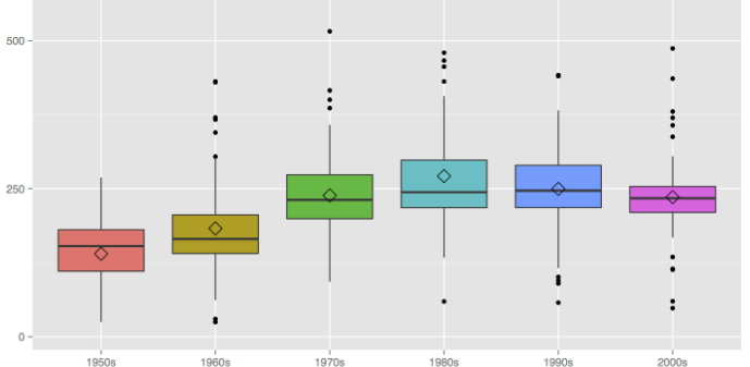
Figure 7: Boxplot of recorded song duration given decade. Note the increase in song duration given decade.

3.3 Quantitative relationships

Quantitative relationships between descriptors can be visualized with graphs, normally limited to 3 dimensions, as it is not easy for humans to visualize data in more than just a few dimensions. Quantitative relationships can clarify the understanding of the correlation, linear or non-linear, between two or more variables. In music, it is very common for one of these variables to be time.

The numerical relationships between descriptors can be summarized with single quantities or equations, e. g. correlation, the slope of a line or the average length of events. This information can be visualized with matrices and graphs, line or scatter. Matrices and graphs can provide fast access to understanding information and relationships between descriptors. Consider visualizing the rhtyhmic density of a solo over time, or a matrix that displays the correlation between music styles: whereas the first provides a visualization that can describe form according to rhythmic descriptors, the second can provide visualization of hidden style groupings.

Quantitative information can also be described using Polar notation. Polar notation is commonly used to display operations between vectors, to display phase in audio signals and, naturally, time in watches. In figure 8 we illustrate the benefit of visualizing correlations with polar notation to validate correlation matrices.

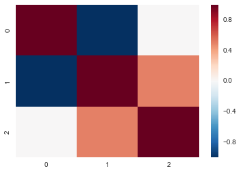
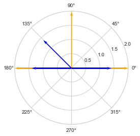
Figure 8: Matrix and polar visualization of correlation between variables 0, 1 and 2. Although the correlation matrix seems correct, a polar visualization immediately shows that the correlations are not valid.

3.4 Qualitative relationships

Qualitative relationships between descriptors can be visualized with diagrams, for example. Borrowing from mathematics, one can describe qualitative relationships with a graph that is comprised by a set of nodes and connections between nodes called edges. Each node can describe a state, e. g. a quantity, object or action and the edges between the states can describe a qualitative or quantitative relationship between the states, e.g. a direct transition or ownership.

In music analysis, it is common to represent the states as pitches, durations or some symbollic encoding of audio; the edges usually represent possible transition from one state to another. Note that a transition does not need to be bidirectional, that is, a transition from A to B does not imply a transition from B to A. Figure 9 shows a graph used by Michel Philippot to compose the first movement of his piece Composition for Double Orchestra.

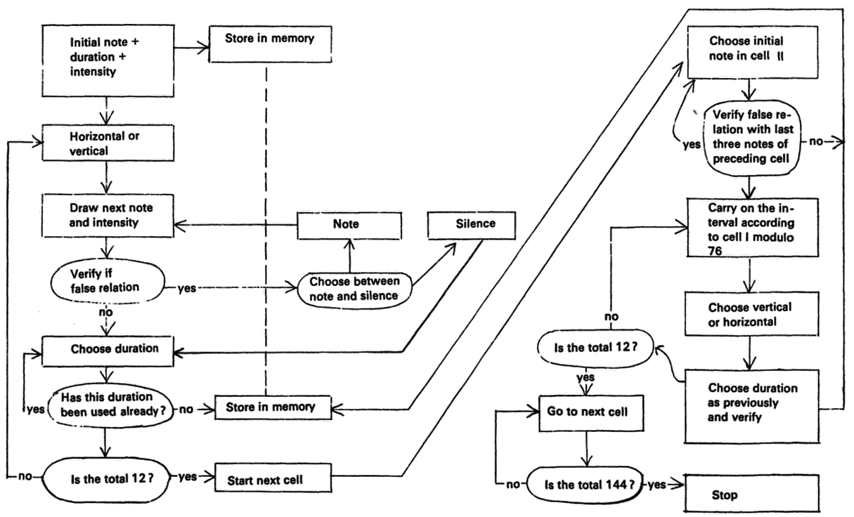
Figure 9: 1945.

4 Software and Datasets

In this section we introduce free computer programs and libraries that can be used in computer aided music analysis. Although most of these programs are dedicated to either symbolic music formats, e.g. MIDI, or Audio, there a few exceptions that operate on both domains.

In the past decades, several programs for computer aided musVic analysis and composition have been designed. IRCAM’s Open Music and its ancestor Music V are such programs that were used in computer aided composition and analysis [3], though their focus has been on music composition. David Huron’s Humdrum [12] is still active nowadays and is one of the pioneer’s in musical analysis using algorithms based on human cognition. Music 21 [9] by Michael Cuthbert from MIT is a python based software for symbolic music analysis with a rather active user base. In addition to supporting multiple file formats, such as XML, humdrum, and MIDI, it has a vast amount of routines that produce low level descriptors and analytical results, related to scales, chords, key and harmonic analysis, pitch and duration summaries and others. Similar to Music 21, pretty_midi [19] by Google Brain’s Colin Raffel is a light-weight and very efficient python library for extracting low level descriptors such as key, meter, pitch and duration from MIDI files or computing descriptors that are usually associated with audio, such as CQT and Chromagrams.

Librosa [15], madmom [5], essentia [6] and marsyas [25] are libraries for retrieving and visualizing information from audio. They are associated with the respective universities or research labs they come from. These libraries provide a large collection of routines that allow users to extract low level descriptors, analyze audio and build statistical models.

Although the programs mentioned in this section require users to have some knowledge of computer programming, this initial cost is usually amortized by end-to-end tutorials, where the users learn, for example, how to write code to extract the key from an audio file or to create a toy model for genre classification using audio data.

5 Applications

This section showcases a few techniques used in music information retrieval and visualization. We forward the interested readers to the proceedings of the International Society for Music Information Retrieval (ISMIR), conferences and the ISMIR mailing list.

5.1 Data abstraction

We informally describe a data abstraction as a function, e.g. an equation or algorithm, that maps an abstract source object onto another object that summarizes the information on the source object, e. g. timbre density is a data abstraction of timbre as shown in Figure 10.

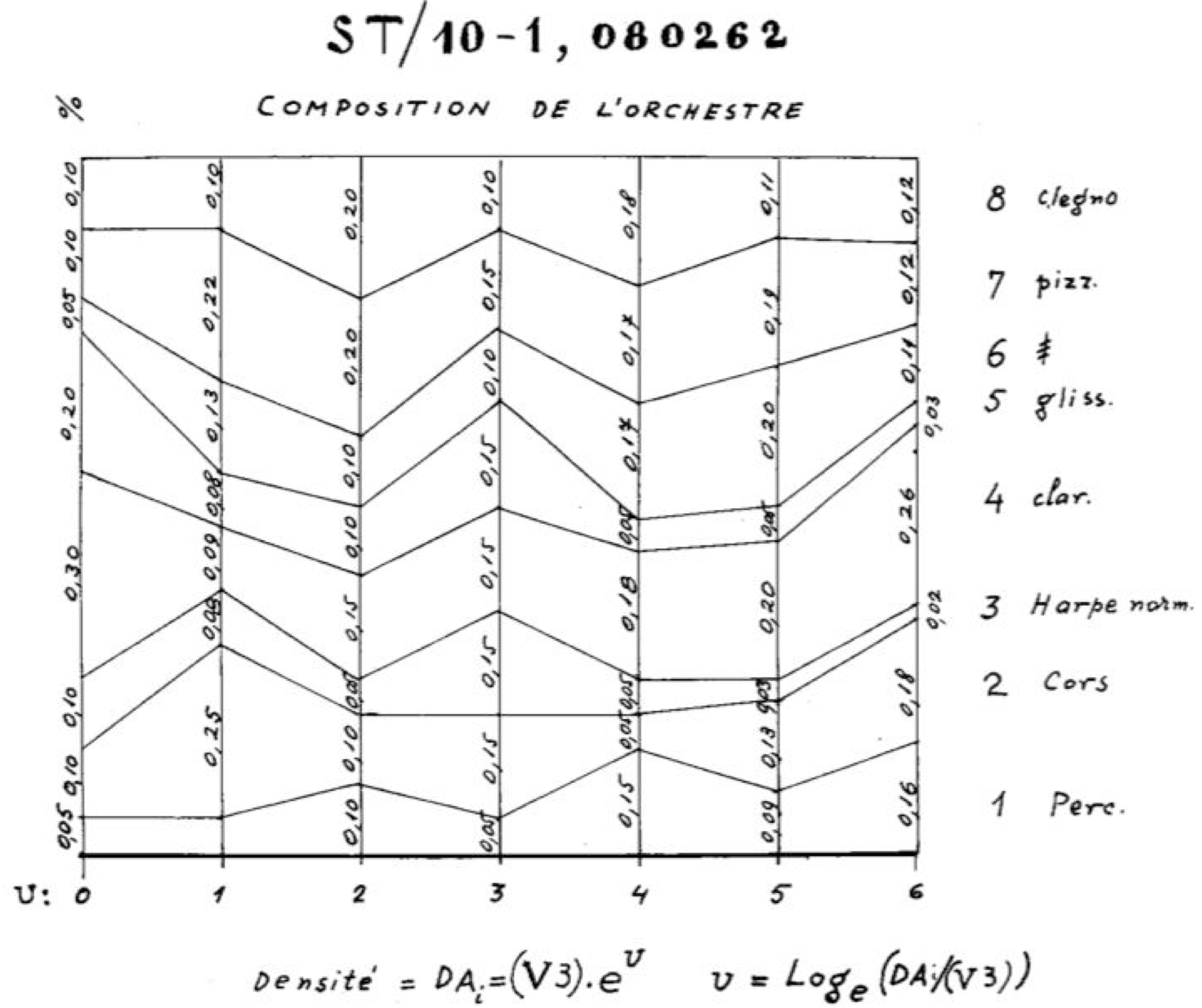
Figure 10: Timbre density in Xenakis’ ST.

A common data abstraction in computational music information retrieval are pitch profiles, which refer to histograms or distributions of pitches. For example, Katy C. Noland and Mark B. Sandler have computationally summarized the energy on pitch classes in major or minor pieces of Bach’s Well Tempered Clavier and used each summary to create pitch class profiles that were associated with the major and minor modes[16]. Following Noland’s approach, other researchers have used MIDI files to compute the frequency of transitions between pitch classes and create pitch class transition profiles that were associated with the key and mode from which they were extracted. In addition to providing a visualization of the distribution of pitch classes, such as Figure 6, and pitch transition, these distribution have been used as features to build key, harmony and chord classifiers.

5.2 Specifications and Automata

Figure 9 describes a graph that has been used to compose a piece of music. The graph in Figure 12 can be used to describe the specifications of a song, loosely speaking, the patterns that are valid or characteristic of a song. More formally, a pattern graph is a labelled directed multigraph whose nodes are values of the descriptors it refers to. A node can be labelled as a starting node, an ending node, or neither. Edges can be labelled with a word that describes the pattern between nodes and a count indicating how many times the pattern occurred. For example, an edge (a, b) labelled (F, 2) in the pattern graph means the pattern a F b occurred 2 times. The complete example of a pattern graph in Figure 12, where we have indicated starting nodes with an unlabelled incoming arrow and ending nodes with a double circle, illustrates specifications a blues song in Figure 11.

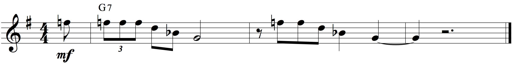
Figure 11: First phrase of Crossroads Blues by Robert Johnson as transcribed in the Real Book of Blues. The transition from chord degree 10 (note f) to chord degree 7 (note d) is always preceded by two or several occurrences of chord degree 10.

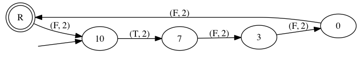
Figure 12: Pattern graph learned on the chord degree feature (interval from root) extracted from the phrase in Fig. 11. The F pattern between chord degrees 10 and 7 has been merged into the pattern 10 T 7.

Graphs visualizations are common amongst researchers working with graphical models and oracles. The Infinite Jukebox shown in Figure 13 is an example of such. Note that as the number of states and edges increases, such graphs become significantly complex, requiring careful attention during visual analysis or making it unfeasible.

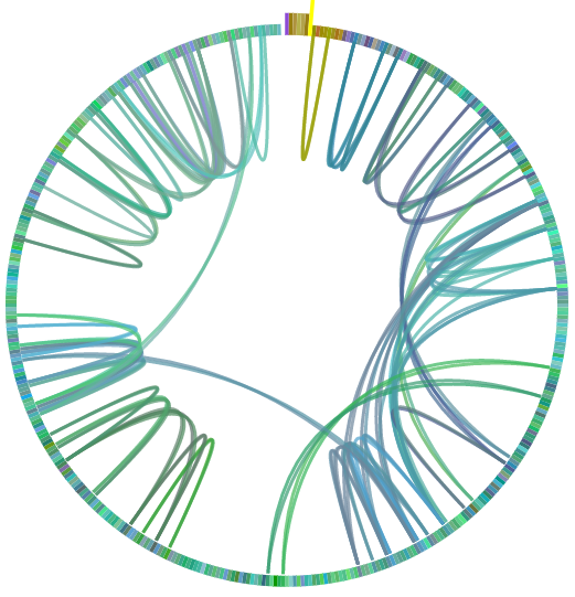
Figure 13: Infinite Jukebox built on the song Supersticion by Stevie Wonder

5.3 Structure Analysis

5.3.1 3D Plots

A visualization of the CQT over time, such as Figure 3, can facilitate the visualization of the structure of a piece. Another visualization that provides information about the structure of a piece are 3D plots, which require mechanisms to project the data abstraction onto a 3D space and to embed temporal information into the plot.

An explicit mechanism to embed temporal information is to annotate each data point in the plot with its order of appeareance. With this, the order can be retrieved by simply following the numerical order. Figure 14 shows such plot and the inevitable cluttering with many data points.

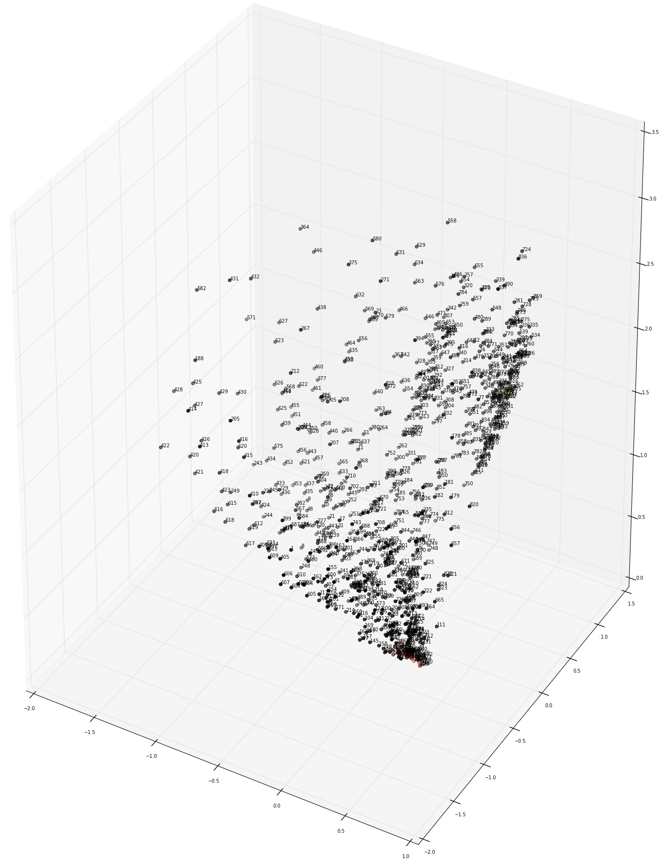
Figure 14: Grisey’s Partiels SVD(CQT)

An implicit mechanism to embed temporal information consists in low-pass filtering (LPF) the data: LPFs can be used to bleed information from previous data frames to the current data frame. In a plot visualization such as Figure 15, this creates a trajectory that produces an implicit visualization of the temporal sequence of the data points.

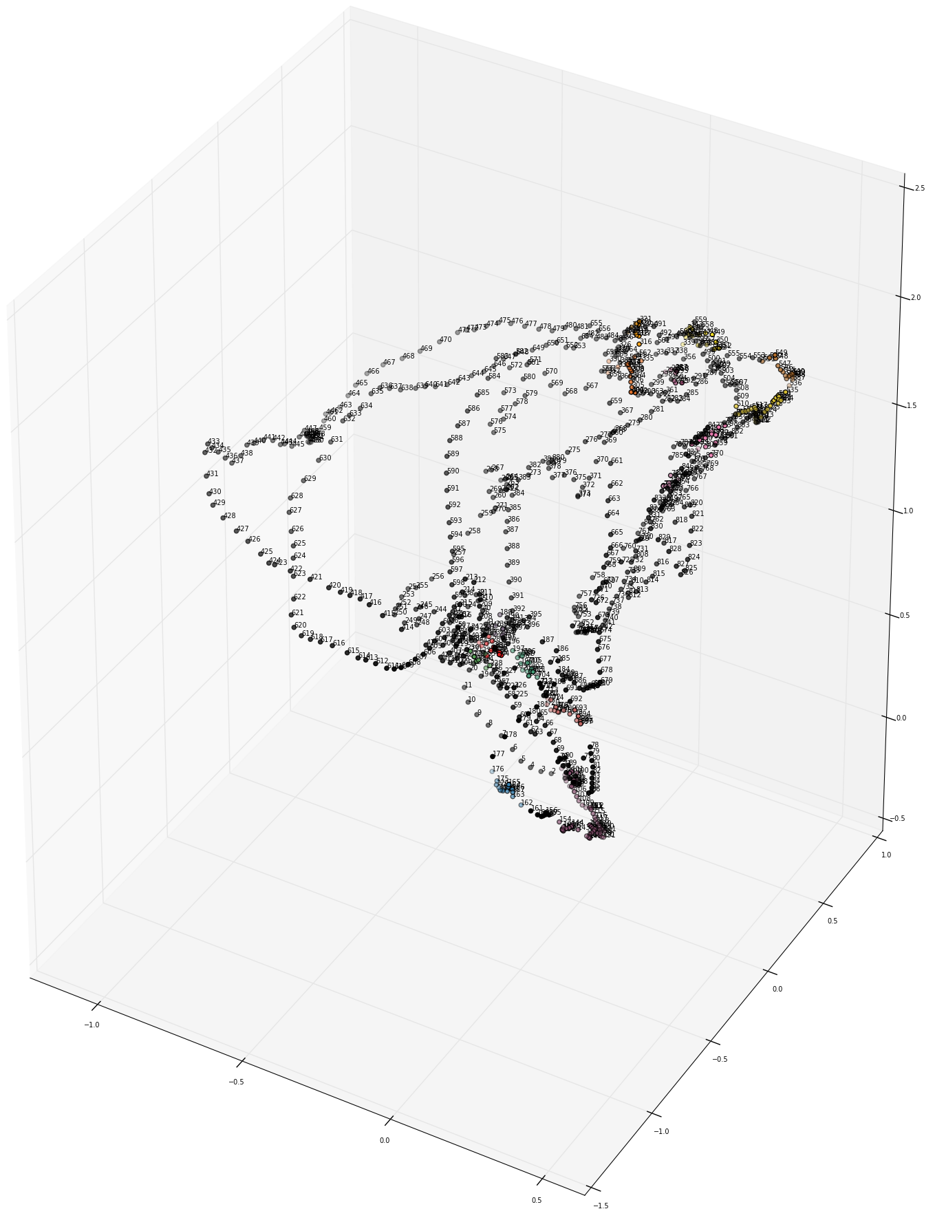
Figure 15: Grisey’s Partiels LPF(SVD(CQT))

5.3.2 Color sequence

Features like the CQT and Chroma can be used by the music specialist to identify patterns in the music. For the enthusiast or novice, a color sequence might be more indicative of similarities and form in music.

Dimensionality reduction can be used to project any feature, for example the CQT with 88 dimensions, to the number of dimensions of a color scheme, for example the RGB color scheme has 3 dimensions: red, green and blue.

In Figure 16, we provide a visualization where CQT features where projected onto a 3D space. After proper scalling, the projected data can then be interpreted and visualized as an image in RGB, where the temporal sequence of colors is directly mapped to the temporal sequence of music, and the similarity in color corresponds to similarity in music, as described by the feature projected onto the color space.

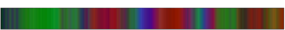
Figure 16: Grisey’s Partiels Color Sequence Based on LPF(SVD(CQT)).

5.3.3 Self-similarity matrices

Self-Similarity Matrices have been used as the main feature for computational structure segmentation. They describe the similarity, as described by some distance function, between all frames  in a music piece. The self-similarity matrix is square and symmetric on the diagonals, that is, the matrix can be divided into two equal triangles.

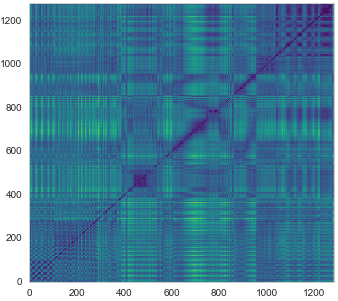
Figure 17: Grisey’s Partiel Self Similarity Matrix computed using Beat-Aligned CQT

5.4 Similarity

Similarity between musical entities is an important subject in music research. Computation enables systematic quantification of similarity between musical entities as described by the features and distance measures designed.

5.4.1 Feature choice and distance measure

To illustrate the importance of the feature choice, let’s consider a musical melody of reference, its octave above and diminished fifth above transposition, named $C_{r}$, $C_{o}$ and $C_{f}$ respectively. Whereas some people people would claim that $C_{o}$ is the most similar to $C_{r}$ because the octave is a more consonant interval, other people would say that $C_{f}$ is the most similar because it has a smaller absolute distance. If, however, the feature used was the sequence of intervals, the melodies would be considered similar to each other.

Now, to illustrate the importance of the distance measure, let’s consider tree pitch profiles $P_{r}$ (C, E, G at 50% volume), $P_{1}$ (no notes), and $P_{2}$(C, E, G at 100% volume). Let’s define our distance measure as the Euclidean distance, $d(x,y)=\sqrt{\sum_{i=1}^{n}(x_{i}-y_{i})^{2}}$. Since the euclidean distance measures the point to point distance between the frequency of each pitch class in the pitch class profiles, the distances d($P_{1}$, $P_{r}$) and d($P_{2}$, $P_{r}$) are exactly the same. On the other hand, musicians would use a distance measure that is more similar to computing the correlation between profiles and say that $P_{2}$ is closer to $P_{r}$ than $P_{1}$)

5.4.2 Similarity Spaces

Given features computed over time windows, i.e. frames, that describe musical entities, computational means can be used to visualize this data and quantify the distances between these frames. The frames could provide, for example, per beat information about some spectral descriptor, e.g. brightness, of songs. One could then plot these frames and their respective brightness and compare, for example, different songs or sections of the same song.

As mentioned before, visualization of data in more than 3 dimensions is hard and will require a mechanism, dimensionality reduction or creative plotting, to reduce the dimensionality of the data or find other ways of plotting it, e.g. using color and shapes to represent other dimensions in the data.

There are several methods for performing dimensionality reduction, including Multidimensional Scaling (MDS), Principal Component Analysis (PCA) and t-SNE, to cite a few. In the late 70s, David Wessel used Multidimesional Scaling to create a timbre space where the distance between points were related to the timbral distance between instruments[26].

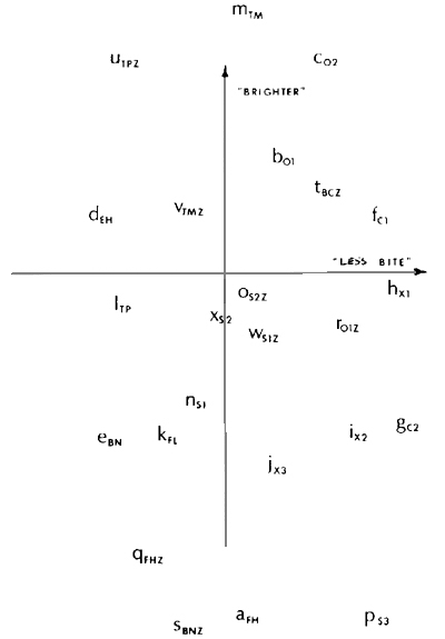
Figure 18: Two-dimensional timbre space representation of 24 instrument-like sounds obtained from Grey.

Unlike MDS and PCA, t-SNE is a dimensionality reduction technique that, informally speaking, tries to preserve in the projected low-dimensional space the distances between points in high-dimensional space.

Figure 19 shows a 2D t-SNE projection of feature frames from thousands of songs. Figure 20 uses the same data as Figure 19 and provides a visualization of median aggregated frames of Hardcore Punk and Ambient songs. Note the clear separation between styles and that the distance between points is a measure of similarity between songs.

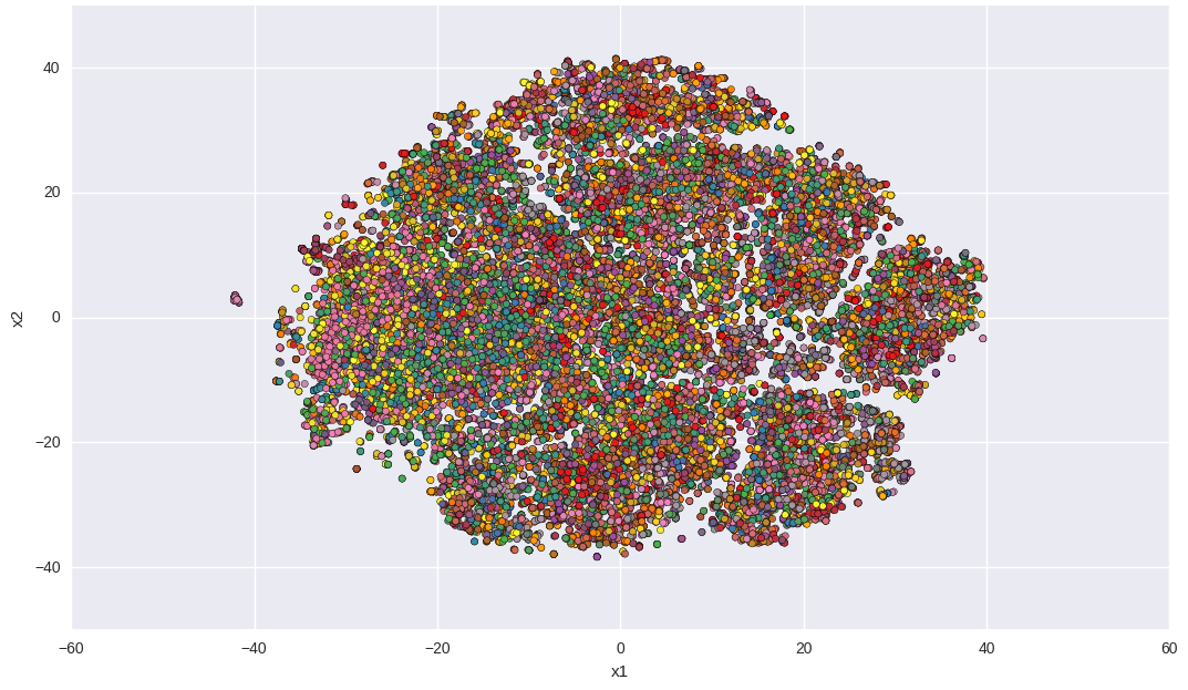
Figure 19: Frame Level Projection

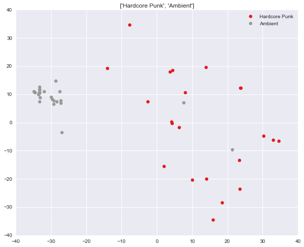
Figure 20: Hardcore and Ambient Projection

6 Conclusions

This paper summarized a few computational strategies for music information retrieval and visualization, including commonly use features and software libraries.. It provided concrete examples of how visualization can be used to retrieve information from music, including abstractions, specifications, structure and similarity.

References

- [1] Theodor W Adorno and Max Paddison. On the problem of musical analysis. Music Analysis, 1(2):169–187, 1982.
- [2] Jonathan Allen. Short term spectral analysis, synthesis, and modification by discrete fourier transform. IEEE Transactions on Acoustics, Speech, and Signal Processing, 25(3):235–238, 1977.
- [3] Gérard Assayag, Camilo Rueda, Mikael Laurson, Carlos Agon, and Olivier Delerue. Computer-assisted composition at ircam: From patchwork to openmusic. Computer Music Journal, 23(3):59–72, 1999.
- [4] Juan Pablo Bello and Jeremy Pickens. A robust mid-level representation for harmonic content in music signals. In ISMIR, volume 5, pages 304–311, 2005.
- [5] Sebastian Böck, Filip Korzeniowski, Jan Schlüter, Florian Krebs, and Gerhard Widmer. madmom: a new python audio and music signal processing library. arXiv preprint arXiv:1605.07008, 2016.
- [6] Dmitry Bogdanov, Nicolas Wack, Emilia Gómez, Sankalp Gulati, Perfecto Herrera, Oscar Mayor, Gerard Roma, Justin Salamon, José R Zapata, and Xavier Serra. Essentia: An audio analysis library for music information retrieval. In ISMIR, pages 493–498. Citeseer, 2013.
- [7] Mark Cartwright, Ayanna Seals, Justin Salamon, Alex Williams, Stefanie Mikloska, Duncan MacConnell, E Law, J Bello, and O Nov. Seeing sound: Investigating the effects of visualizations and complexity on crowdsourced audio annotations. Proceedings of the ACM on Human-Computer Interaction, 1(1), 2017.
- [8] Peter Castine. Set theory objects: abstractions for computer-aided analysis and composition of serial and atonal music. Peter Lang Publishing, 1994.
- [9] Michael Scott Cuthbert and Christopher Ariza. music21: A toolkit for computer-aided musicology and symbolic music data. 2010.
- [10] J Stephen Downie. Music information retrieval. Annual review of information science and technology, 37(1):295–340, 2003.
- [11] Geoffrey Hinton, Li Deng, Dong Yu, George E Dahl, Abdel-rahman Mohamed, Navdeep Jaitly, Andrew Senior, Vincent Vanhoucke, Patrick Nguyen, Tara N Sainath, et al. Deep neural networks for acoustic modeling in speech recognition: The shared views of four research groups. IEEE Signal Processing Magazine, 29(6):82–97, 2012.
- [12] David Huron. Music information processing using the humdrum toolkit: Concepts, examples, and lessons. Computer Music Journal, 26(2):11–26, 2002.
- [13] Cynthia Liem, Meinard Müller, Douglas Eck, George Tzanetakis, and Alan Hanjalic. The need for music information retrieval with user-centered and multimodal strategies. In Proceedings of the 1st international ACM workshop on Music information retrieval with user-centered and multimodal strategies, pages 1–6. ACM, 2011.
- [14] Beth Logan et al. Mel frequency cepstral coefficients for music modeling. In ISMIR, volume 270, pages 1–11, 2000.
- [15] Brian McFee, Colin Raffel, Dawen Liang, Daniel PW Ellis, Matt McVicar, Eric Battenberg, and Oriol Nieto. librosa: Audio and music signal analysis in python. In Proceedings of the 14th Python in Science Conference, 2015.
- [16] Katy Noland and Mark Sandler. Signal processing parameters for tonality estimation. In Audio Engineering Society Convention 122. Audio Engineering Society, 2007.
- [17] Geoffroy Peeters. A large set of audio features for sound description (similarity and classification) in the cuidado project. 2004.
- [18] Matthew Prockup, Andreas F Ehmann, Fabien Gouyon, Erik M Schmidt, Oscar Celma, and Youngmoo E Kim. Modeling genre with the music genome project: Comparing human-labeled attributes and audio features. In ISMIR, pages 31–37, 2015.
- [19] Colin Raffel and Daniel PW Ellis. Intuitive analysis, creation and manipulation of midi data with pretty_midi. In Proceedings of the 15th International Society for Music Information Retrieval Conference Late Breaking and Demo Papers, 2014.
- [20] Amit Singhal. Modern information retrieval: A brief overview. IEEE Data Eng. Bull., 24(4):35–43, 2001.
- [21] Trisha and Arianna. Mozart Visual Representation, 2013 (accessed July 26, 2018).
- [22] Trisha and Arianna. An analysis of music hits across decades: 1950-2009, 2016 (accessed July 26, 2018).
- [23] Edward R Tufte and PR Graves-Morris. The visual display of quantitative information, volume 2. Graphics press Cheshire, CT, 1983.
- [24] Rainer Typke, Frans Wiering, Remco C Veltkamp, et al. A survey of music information retrieval systems. In ISMIR, pages 153–160, 2005.
- [25] George Tzanetakis and Perry Cook. Marsyas: A framework for audio analysis. Organised sound, 4(3):169–175, 2000.
- [26] David L Wessel. Timbre space as a musical control structure. Computer music journal, pages 45–52, 1979.