Superpixel Sampling Networks

Abstract

Superpixels provide an efficient low/mid-level representation of image data, which greatly reduces the number of image primitives for subsequent vision tasks. Existing superpixel algorithms are not differentiable, making them difficult to integrate into otherwise end-to-end trainable deep neural networks. We develop a new differentiable model for superpixel sampling that leverages deep networks for learning superpixel segmentation. The resulting Superpixel Sampling Network (SSN) is end-to-end trainable, which allows learning task-specific superpixels with flexible loss functions and has fast runtime. Extensive experimental analysis indicates that SSNs not only outperform existing superpixel algorithms on traditional segmentation benchmarks, but can also learn superpixels for other tasks. In addition, SSNs can be easily integrated into downstream deep networks resulting in performance improvements.

1 Introduction

Superpixels are an over-segmentation of an image that is formed by grouping image pixels [33] based on low-level image properties. They provide a perceptually meaningful tessellation of image content, thereby reducing the number of image primitives for subsequent image processing. Owing to their representational and computational efficiency, superpixels have become an established low/mid-level image representation and are widely-used in computer vision algorithms such as object detection [35, 42], semantic segmentation [15, 34, 13], saliency estimation [18, 30, 43, 46], optical flow estimation [20, 28, 37, 41], depth estimation [6], tracking [44] to name a few. Superpixels are especially widely-used in traditional energy minimization frameworks, where a low number of image primitives greatly reduce the optimization complexity.

The recent years have witnessed a dramatic increase in the adoption of deep learning for a wide range of computer vision problems. With the exception of a few methods (e.g., [13, 18, 34]), superpixels are scarcely used in conjunction with modern deep networks. There are two main reasons for this. First, the standard convolution operation, which forms the basis of most deep architectures, is usually defined over regular grid lattices and becomes inefficient when operating over irregular superpixel lattices. Second, existing superpixel algorithms are non-differentiable and thus using superpixels in deep networks introduces non-differentiable modules in otherwise end-to-end trainable network architectures.

In this work, we alleviate the second issue by proposing a new deep differentiable algorithm for superpixel segmentation. We start by revisiting the widely-used Simple Linear Iterative Clustering (SLIC) superpixel algorithm [1] and turn it into a differentiable algorithm by relaxing the nearest neighbor constraints present in SLIC. This new differentiable algorithm allows for end-to-end training and enables us to leverage powerful deep networks for learning superpixels instead of using traditional hand-crafted features. This combination of a deep network with differentiable SLIC forms our end-to-end trainable superpixel algorithm which we call Superpixel Sampling Network (SSN). Fig. 1 shows an overview of the proposed SSN. A given input image is first passed through a deep network producing features at each pixel. These deep features are then passed onto the differentiable SLIC, which performs iterative clustering, resulting in the desired superpixels. The entire network is end-to-end trainable. The differentiable nature of SSN allows the use of flexible loss functions for learning task-specific superpixels. Fig. 1 shows some sample SSN generated superpixels.

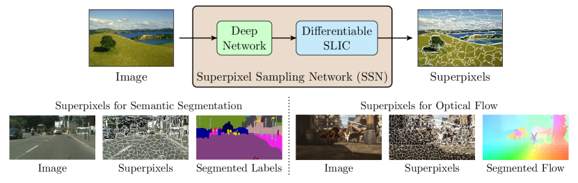
Figure 1: Overview of Superpixel Sampling Networks. A given image is first passed onto a deep network that extracts features at each pixel, which are then used by differentiable SLIC to generate the superpixels. Shown here are a couple of example SSN generated task-specific superpixels for semantic segmentation and optical flow.

Experimental results on 3 different segmentation benchmark datasets including BSDS500 [4], Cityscapes [10] and PascalVOC [11] indicate that the proposed superpixel sampling network (SSN) performs favourably against existing prominent superpixel algorithms, while also being faster. We also demonstrate that by simply integrating our SSN framework into an existing semantic segmentation network [13] that uses superpixels, performance improvements are achieved. In addition, we demonstrate the flexibility of SSN in learning superpixels for other vision tasks. Specifically, in a proof-of-concept experiment on the Sintel optical flow dataset [7], we demonstrate how we can learn superpixels that better align with optical flow boundaries rather than standard object boundaries. The proposed SSN has the following favorable properties in comparison to existing superpixel algorithms:

• End-to-end trainable: SSNs are end-to-end trainable and can be easily integrated into other deep network architectures. To the best of our knowledge, this is the first end-to-end trainable superpixel algorithm.

• Flexible and task-specific: SSN allows for learning with flexible loss functions resulting in the learning of task-specific superpixels.

• State-of-the-art performance: Experiments on a wide range of benchmark datasets show that SSN outperforms existing superpixel algorithms.

• Favorable runtime: SSN also performs favorably against prominent superpixel algorithms in terms of runtime, making it amenable to learn on large datasets and also effective for practical applications.

2 Related Work

Superpixel algorithms. Traditional superpixel algorithms can be broadly classified into graph-based and clustering-based approaches. Graph-based approaches formulate the superpixel segmentation as a graph-partitioning problem where graph nodes are represented by pixels and the edges denote the strength of connectivity between adjacent pixels. Usually, the graph partitioning is performed by solving a discrete optimization problem. Some widely-used algorithms in this category include the normalized-cuts [33], Felzenszwalb and Huttenlocher (FH) [12], and the entropy rate superpixels (ERS) [26]. As discrete optimization involves discrete variables, the optimization objectives are usually non-differentiable making it difficult to leverage deep networks in graph-based approaches.

Clustering-based approaches, on the other hand, leverage traditional clustering techniques such as $k$-means for superpixel segmentation. Widely-used algorithms in this category include SLIC [1], LSC [25], and Manifold-SLIC [27]. These methods mainly do $k$-means clustering but differ in their feature representation. While the SLIC [1] represents each pixel as a $5$-dimensional positional and Lab color features ($XYLab$ features), LSC [25] method projects these $5$-dimensional features on to a $10$-dimensional space and performs clustering in the projected space. Manifold-SLIC [27], on the other hand, uses a $2$-dimensional manifold feature space for superpixel clustering. While these clustering algorithms require iterative updates, a non-iterative clustering scheme for superpixel segmentation is proposed in the SNIC method [2]. The proposed approach is also a clustering-based approach. However, unlike existing techniques, we leverage deep networks to learn features for superpixel clustering via an end-to-end training framework.

As detailed in a recent survey paper [36], other techniques are used for superpixel segmentation, including watershed transform [29], geometric flows [24], graph-cuts [39], mean-shift [9], and hill-climbing [5]. However, these methods all rely on hand-crafted features and it is non-trivial to incorporate deep networks into these techniques. A very recent technique of SEAL [38] proposed a way to learn deep features for superpixel segmentation by bypassing the gradients through non-differentiable superpixel algorithms. Unlike our SSN framework, SEAL is not end-to-end differentiable.

Deep clustering. Inspired by the success of deep learning for supervised tasks, several methods investigate the use of deep networks for unsupervised data clustering. Recently, Greff et. al. [17] propose the neural expectation maximization framework where they model the posterior distribution of cluster labels using deep networks and unroll the iterative steps in the EM procedure for end-to-end training. In another work [16], the Ladder network [31] is used to model a hierarchical latent variable model for clustering. Hershey et. al. [19] propose a deep learning-based clustering framework for separating and segmenting audio signals. Xie et. al. [40] propose a deep embedded clustering framework, for simultaneously learning feature representations and cluster assignments. In a recent survey paper, Aljalbout et. al. [3] give a taxonomy of deep learning based clustering methods. In this paper, we also propose a deep learning-based clustering algorithm. Different from the prior work, our algorithm is tailored for the superpixel segmentation task where we use image-specific constraints. Moreover, our framework can easily incorporate other vision objective functions for learning task-specific superpixel representations.

3 Preliminaries

At the core of SSN is a differentiable clustering technique that is inspired by the SLIC [1] superpixel algorithm. Here, we briefly review the SLIC before describing our SSN technique in the next section. SLIC is one of the simplest and also one of the most widely-used superpixel algorithms. It is easy to implement, has fast runtime and also produces compact and uniform superpixels.

Although there are several different variants [25, 27] of SLIC algorithm, in the original form, SLIC is a k-means clustering performed on image pixels in a five dimensional position and color space (usually scaled $XYLab$ space). Formally, given an image $I\in\mathbb{R}^{n\times 5}$, with $5$-dimensional $XYLab$ features at $n$ pixels, the task of superpixel computation is to assign each pixel to one of the $m$ superpixels i.e., to compute the pixel-superpixel association map $H\in\{0,1,\cdots,m-1\}^{n\times 1}$. The SLIC algorithm operates as follows. First, we sample initial cluster (superpixel) centers $S^{0}\in\mathbb{R}^{m\times 5}$ in the $5$-dimensional space. This sampling is usually done uniformly across the pixel grid with some local perturbations based on image gradients. Given these initial superpixel centers $S^{0}$, the SLIC algorithm proceeds in an iterative manner with the following two steps in each iteration $t$:

1. Pixel-Superpixel association: Associate each pixel to the nearest superpixel center in the five-dimensional space, i.e., compute the new superpixel assignment at each pixel $p$,

   $$H_{p}^{t}=\underset{i\in\{0,...,m-1\}}{\arg\min}D(I_{p},S^{t-1}_{i}),$$ (1)

   where $D$ denotes the distance computation $D(\textbf{a},\textbf{b})=||\textbf{a}-\textbf{b}||^{2}$.

2. Superpixel center update: Average pixel features ($XYLab$) inside each superpixel cluster to obtain new superpixel cluster centers $S^{t}$. For each superpixel $i$, we compute the centroid of that cluster,

   $$S^{t}_{i}=\frac{1}{Z_{i}^{t}}\sum_{p|H_{p}^{t}=i}I_{p},$$ (2)

   where $Z_{i}^{t}$ denotes the number of pixels in the superpixel cluster $i$.

These two steps form the core of the SLIC algorithm and are repeated until either convergence or for a fixed number of iterations. Since computing the distance $D$ in Eq. 1 between all the pixels and superpixels is time-consuming, this computation is usually constrained to a fixed neighborhood around each superpixel center. At the end, depending on the application, there is an optional step of enforcing spatial connectivity across pixels in each superpixel cluster. More details regarding the SLIC algorithm can be found in Achanta et. al. [1]. In the next section, we elucidate how we modify the SLIC algorithm to develop SSN.

4 Superpixel Sampling Networks

As illustrated in Fig. 1, SSN is composed of two parts: A deep network that generates pixel features, which are then passed on to differentiable SLIC. Here, we first describe the differentiable SLIC followed by the SSN architecture.

4.1 Differentiable SLIC

Why is SLIC not differentiable? A closer look at all the computations in SLIC shows that the non-differentiability arises because of the computation of pixel-superpixel associations, which involves a non-differentiable nearest neighbor operation. This nearest neighbor computation also forms the core of the SLIC superpixel clustering and thus we cannot avoid this operation.

A key to our approach is to convert the nearest-neighbor operation into a differentiable one. Instead of computing hard pixel-superpixel associations $H\in\{0,1,\cdots,m-1\}^{n\times 1}$ (in Eq. 1), we propose to compute soft-associations $Q\in\mathbb{R}^{n\times m}$ between pixels and superpixels. Specifically, for a pixel $p$ and superpixel $i$ at iteration $t$, we replace the nearest-neighbor computation (Eq. 1) in SLIC with the following pixel-superpixel association.

$$Q_{pi}^{t}=e^{-D(I_{p},S_{i}^{t-1})}=e^{-||I_{p}-S_{i}^{t-1}||^{2}}$$ (3)

Correspondingly, the computation of new superpixels cluster centers (Eq. 2) is modified as the weighted sum of pixel features,

$$S^{t}_{i}=\frac{1}{Z_{i}^{t}}\sum_{p=1}^{n}Q_{pi}^{t}I_{p},$$ (4)

where $Z_{i}^{t}=\sum_{p}Q_{pi}^{t}$ is the normalization constant. For convenience, we refer to the column normalized $Q^{t}$ as $\hat{Q^{t}}$ and thus we can write the above superpixel center update as $S^{t}=\hat{Q^{t}}^{\top}I$. The size of $Q$ is $n\times m$ and even for a small number of superpixels $m$, it is prohibitively expensive to compute $Q_{pi}$ between all the pixels and superpixels. Therefore, we constrain the distance computations from each pixel to only 9 surrounding superpixels as illustrated using the red and green boxes in Fig. 2. For each pixel in the green box, only the surrounding superpixels in the red box are considered for computing the association. This brings down the size of $Q$ from $n\times m$ to $n\times 9$, making it efficient in terms of both computation and memory. This approximation in the $Q$ computation is similar in spirit to the approximate nearest-neighbor search in SLIC.

Figure 2: From initial grid to learned superpixels. An example visual result from BSDS500 dataset showing the initial superpixel grid and the superpixels obtained with SSN_pix and SSN_deep. To compute the pixel-superpixel associations for every pixel in the green box, only the surrounding superpixels in the red box are considered.

Algorithm 1 Superpixel Sampling Network (SSN)

1:Input: Image $\underset{n\times 5}{I}$. $\triangleright$ $XYLab$ features

2:Output: Pixel-Superpixel association $\underset{n\times m}{Q}$.

3:Pixel features using a CNN, $\underset{n\times k}{F}=\mathcal{F}(I)$.

4:Initial superpixel centers with average features in regular grid cells, $\underset{m\times k}{S^{0}}=\mathcal{J}(F)$.

5:for each iteration $t$ in $1$ to $v$ do

6:     Compute association between each pixel $p$ and the surrounding superpixel $i$, $Q_{pi}^{t}=e^{-||F_{p}-S_{i}^{t-1}||^{2}}$.

7:     Compute new superpixel centers, $S^{t}_{i}=\frac{1}{Z_{i}^{t}}\sum_{p=1}^{n}Q_{pi}^{t}F_{p}$; $Z_{i}^{t}=\sum_{p}Q_{pi}^{t}$.

8:end for

9:(Optional) Compute hard-associations $\underset{n\times 1}{H^{v}};H_{p}^{v}=\underset{i\in\{0,...,m-1\}}{\arg\max}Q_{pi}^{v}$.

10:(Optional) Enforce spatial connectivity.

Now, both the computations in each SLIC iteration are completely differentiable and we refer to this modified algorithm as differentiable SLIC. Empirically, we observe that replacing the hard pixel-superpixel associations in SLIC with the soft ones in differentiable SLIC does not result in any performance degradations. Since this new superpixel algorithm is differentiable, it can be easily integrated into any deep network architecture. Instead of using manually designed pixel features $I_{p}$, we can leverage deep feature extractors and train the whole network end-to-end. In other words, we replace the image features $I_{p}$ in the above computations (Eq. 3 and 4) with $k$ dimensional pixel features $F_{p}\in\mathbb{R}^{n\times k}$ computed using a deep network. We refer to this coupling of deep networks with the differentiable SLIC as Superpixel Sampling Network (SSN).

Algorithm 1 outlines all the computation steps in SSN. The algorithm starts with deep image feature extraction using a CNN (line 1). We initialize the superpixel cluster centers (line 2) with the average pixels features in an initial regular superpixel grid (Fig. 2). Then, for $v$ iterations, we iteratively update pixel-superpixel associations and superpixel centers, using the above-mentioned computations (lines 3-6). Although one could directly use soft pixel-superpixel associations $Q$ for several downstream tasks, there is an optional step of converting soft associations to hard ones (line 7), depending on the application needs. In addition, like in the original SLIC algorithm, we can optionally enforce spatial connectivity across pixels inside each superpixel cluster. This is accomplished by merging the superpixels, smaller than certain threshold, with the surrounding ones and then assigning a unique cluster ID for each spatially-connected component. Note that these two optional steps (lines 7, 8) are not differentiable.

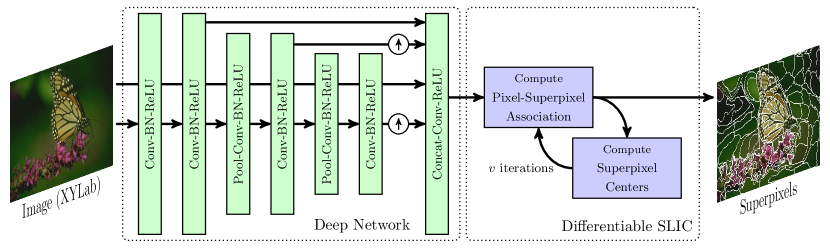
Figure 3: Computation flow of SSN. Our network is composed of a series of convolution layers interleaved with Batch Norm (BN) and ReLU nonlinearities. $\uparrow$ denotes bilinear upsampling to the original image resolution. The features from CNNs are then passed onto iterative updates in the differentiable SLIC to generate superpixels.

Mapping between pixel and superpixel representations. For some downstream applications that use superpixels, pixel representations are mapped onto superpixel representations and vice versa. With the traditional superpixel algorithms, which provide hard clusters, this mapping from pixel to superpixel representations is done via averaging inside each cluster (Eq. 2). The inverse mapping from superpixel to pixel representations is done by assigning the same superpixel feature to all the pixels belonging to that superpixel. We can use the same pixel-superpixel mappings with SSN superpixels as well, using the hard clusters (line 7 in Algorithm 1) obtained from SSN. However, since this computation of hard-associations is not differentiable, it may not be desirable to use hard clusters when integrating into an end-to-end trainable system. It is worth noting that the soft pixel-superpixel associations generated by SSN can also be easily used for mapping between pixel and superpixel representations. Eq. 4 already describes the mapping from a pixel to superpixel representation which is a simple matrix multiplication with the transpose of column-normalized $Q$ matrix: $S=\hat{Q}^{\top}F$, where $F$ and $S$ denote pixel and superpixel representations respectively. The inverse mapping from superpixel to pixel representation is done by multiplying the row-normalized $Q$, denoted as $\tilde{Q}$, with the superpixel representations, $F=\tilde{Q}S$. Thus the pixel-superpixel feature mappings are given as simple matrix multiplications with the association matrix and are differentiable. Later, we will make use of these mappings in designing the loss functions to train SSN.

4.2 Network Architecture

Fig. 3 shows the SSN network architecture. The CNN for feature extraction is composed of a series of convolution layers interleaved with batch normalization [21] (BN) and ReLU activations. We use max-pooling, which downsamples the input by a factor of 2, after the 2^nd and 4^th convolution layers to increase the receptive field. We bilinearly upsample the 4^th and 6^th convolution layer outputs and then concatenate with the 2^nd convolution layer output to pass onto the final convolution layer. We use $3\times 3$ convolution filters with the number of output channels set to 64 in each layer, except the last CNN layer which outputs $k-5$ channels. We concatenate this $k-5$ channel output with the $XYLab$ of the given image resulting in $k$-dimensional pixel features. We choose this CNN architecture for its simplicity and efficiency. Other network architectures are conceivable. The resulting $k$ dimensional features are passed onto the two modules of differentiable SLIC that iteratively updates pixel-superpixel associations and superpixel centers for $v$ iterations. The entire network is end-to-end trainable.

4.3 Learning Task-Specific Superpixels

One of the main advantages of end-to-end trainable SSN is the flexibility in terms of loss functions, which we can use to learn task-specific superpixels. Like in any CNN, we can couple SSN with any task-specific loss function resulting in the learning of superpixels that are optimized for downstream computer vision tasks. In this work, we focus on optimizing the representational efficiency of superpixels i.e., learning superpixels that can efficiently represent a scene characteristic such as semantic labels, optical flow, depth etc. As an example, if we want to learn superpixels that are going to be used for downstream semantic segmentation task, it is desirable to produce superpixels that adhere to semantic boundaries. To optimize for representational efficiency, we find that the combination of a task-specific reconstruction loss and a compactness loss performs well.

Task-specific reconstruction loss. We denote the pixel properties that we want to represent efficiently with superpixels as $R\in\mathbb{R}^{n\times l}$. For instance, $R$ can be semantic label (as one-hot encoding) or optical flow maps. It is important to note that we do not have access to $R$ during the test time, i.e., SSN predicts superpixels only using image data. We only use $R$ during training so that SSN can learn to predict superpixels suitable to represent $R$. As mentioned previously in Section 4.1, we can map the pixel properties onto superpixels using the column-normalized association matrix $\hat{Q}$, $\breve{R}=\hat{Q}^{\top}R$, where $\breve{R}\in\mathbb{R}^{m\times l}$. The resulting superpixel representation $\breve{R}$ is then mapped back onto pixel representation $R^{*}$ using row-normalized association matrix $\tilde{Q}$, $R^{*}=\tilde{Q}S$, where $R^{*}\in\mathbb{R}^{n\times l}$. Then the reconstruction loss is given as

$$L_{recon}=\mathcal{L}(R,R^{*})=\mathcal{L}(R,\tilde{Q}\hat{Q}^{\top}R)$$ (5)

where $\mathcal{L}(.,.)$ denotes a task-specific loss-function. In this work, for segmentation tasks, we used cross-entropy loss for $\mathcal{L}$ and used L1-norm for learning superpixels for optical flow. Here $Q$ denotes the association matrix $Q^{v}$ after the final iteration of differentiable SLIC. We omit $v$ for convenience.

Compactness loss. In addition to the above loss, we also use a compactness loss to encourage superpixels to be spatially compact i.e., to have lower spatial variance inside each superpixel cluster. Let $I^{xy}$ denote positional pixel features. We first map these positional features into our superpixel representation, $S^{xy}=\hat{Q}^{\top}I^{xy}$. Then, we do the inverse mapping onto the pixel representation using the hard associations $H$, instead of soft associations $Q$, by assigning the same superpixel positional feature to all the pixels belonging to that superpixel, $\bar{I}_{p}^{xy}=S_{i}^{xy}|H_{p}=i$. The compactness loss is defined as the following L2 norm:

$$L_{compact}=||I^{xy}-\bar{I}^{xy}||_{2}.$$ (6)

This loss encourages superpixels to have lower spatial variance. The flexibility of SSN allows using many other loss functions, which makes for interesting future research. The overall loss we use in this work is a combination of these two loss functions, $L=L_{recon}+\lambda L_{compact}$, where we set $\lambda$ to $10^{-5}$ in all our experiments.

4.4 Implementation and Experiment Protocols

We implement the differentiable SLIC as neural network layers using CUDA in the Caffe neural network framework [22]. All the experiments are performed using Caffe with the Python interface. We use scaled $XYLab$ features as input to the SSN, with position and color feature scales represented as $\gamma_{pos}$ and $\gamma_{color}$ respectively. The value of $\gamma_{color}$ is independent of the number of superpixels and is set to 0.26 with color values ranging between 0 and 255. The value of $\gamma_{pos}$ depends on the number of superpixels, $\gamma_{pos}=\eta\max{(m_{w}/n_{w},m_{h}/n_{h})}$, where $m_{w},n_{w}$ and $m_{h},n_{h}$ denotes the number of superpixels and pixels along the image width and height respectively. In practice, we observe that $\eta=2.5$ performs well.

For training, we use image patches of size $201\times 201$ and $100$ superpixels. In terms of data augmentation, we use left-right flips and for the small BSDS500 dataset [4], we use an additional data augmentation of random scaling of image patches. For all the experiments, we use Adam stochastic optimization [23] with a batch size of $8$ and a learning rate of $0.0001$. Unless otherwise mentioned, we trained the models for 500K iterations and choose the final trained models based on validation accuracy. For the ablation studies, we trained models with varying parameters for 200K iterations. It is important to note that we use a single trained SSN model for estimating varying number of superpixels by scaling the input positional features as described above. We use 5 iterations ($v=5$) of differentiable SLIC for training and used 10 iterations while testing as we observed only marginal performance gains with more iterations. Refer to https://varunjampani.github.io/ssn/ for the code and trained models.

5 Experiments

We conduct experiments on 4 different benchmark datasets. We first demonstrate the use of learned superpixels with experiments on the prominent superpixel benchmark BSDS500 [4] (Section 5.1). We then demonstrate the use of task-specific superpixels on the Cityscapes [10] and PascalVOC [11] datasets for semantic segmentation (Section 5.2), and on MPI-Sintel [7] dataset for optical flow (Section 5.3). In addition, we demonstrate the use of SSN superpixels in a downstream semantic segmentation network that uses superpixels (Section 5.2).

5.1 Learned Superpixels

We perform ablation studies and evaluate against other superpixel techniques on the BSDS500 benchmark dataset [4]. BSDS500 consists of 200 train, 100 validation, and 200 test images. Each image is annotated with ground-truth (GT) segments from multiple annotators. We treat each annotation as as a separate sample resulting in 1633 training/validation pairs and 1063 testing pairs.

In order to learn superpixels that adhere to GT segments, we use GT segment labels in the reconstruction loss (Eq. 5). Specifically, we represent GT segments in each image as one-hot encoding vectors and use that as pixel properties $R$ in the reconstruction loss. We use the cross-entropy loss for $\mathcal{L}$ in Eq. 5. Note that, unlike in the semantic segmentation task where the GT labels have meaning, GT segments in this dataset do not carry any semantic meaning. This does not pose any issue to our learning setup as both the SSN and reconstruction loss are agnostic to the meaning of pixel properties $R$. The reconstruction loss generates a loss value using the given input signal $R$ and its reconstructed version $R^{*}$ and does not consider whether the meaning of $R$ is preserved across images.

Evaluation metrics. Superpixels are useful in a wide range of vision tasks and several metrics exist for evaluating superpixels. In this work, we consider Achievable Segmentation Accuracy (ASA) as our primary metric while also reporting boundary metrics such as Boundary Recall (BR) and Boundary Precision (BP) metrics. ASA score represents the upper bound on the accuracy achievable by any segmentation step performed on the superpixels. Boundary precision and recall on the other hand measures how well the superpixel boundaries align with the GT boundaries. We explain these metrics in more detail in the supplementary material. The higher these scores, the better is the segmentation result. We report the average ASA and boundary metrics by varying the average number of generated superpixels. A fair evaluation of boundary precision and recall expects superpixels to be spatially connected. Thus, for the sake of unbiased comparisons, we follow the optional post-processing of computing hard clusters and enforcing spatial connectivity (lines 7–8 in Algorithm 1) on SSN superpixels.

Ablation studies. We refer to our main model illustrated in Fig. 3, with 7 convolution layers in deep network, as SSN_deep. As a baseline model, we evalute the superpixels generated with differentiable SLIC that takes pixel $XYLab$ features as input. This is similar to standard SLIC algorithm, which we refer to as SSN_pix and has no trainable parameters. As an another baseline model, we replaced the deep network with a single convolution layer that learns to linearly transform input $XYLab$ features, which we refer to as SSN_linear.

Fig. 4 shows the average ASA and BR scores for these different models with varying feature dimensionality $k$ and the number of iterations $v$ in differentiable SLIC. The ASA and BR of SSN_linear is already reliably higher than the baseline SSN_pix showing the importance of our loss functions and back-propagating the loss signal through the superpixel algorithm. SSN_deep further improves ASA and BR scores by a large margin. We observe slightly better scores with higher feature dimensionality $k$ and also more iterations $v$. For computational reasons, we choose $k=20$ and $v=10$ and from here on refer to this model as SSN_deep.

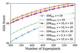
[0pt]      [0pt]

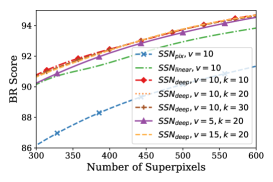
Figure 4: Ablation studies on BSDS500. Results on the test set show that both the ASA and BR scores considerably improve with deep network, and marginally improve with higher number of feature dimensions $k$ and differentiable SLIC iterations $v$.

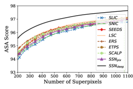
[0pt]      [0pt]

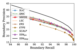
Figure 5: Results on BSDS500 test. SSN performs favourably against other techniques in terms of both ASA score and boundary precision-recall.

Comparison with the state-of-the-arts. Fig. 10 shows the ASA and precision-recall comparison of SSN with state-of-the-art superpixel algorithms. We compare with the following prominent algorithms: SLIC [1], SNIC [2], SEEDS [5], LSC [25], ERS [26], ETPS [45] and SCALP [14]. Plots indicate that SSN_pix performs similarly to SLIC superpixels, showing that the performance of SLIC does not drop when relaxing the nearest neighbor constraints. Comparison with other techniques indicate that SSN performs considerably better in terms of both ASA score and precision-recall. Fig. 2 shows a visual result comparing SSN_pix and SSN_deep and, Fig. 7 shows visual results comparing SSN_deep with state-of-the-arts. Notice that SSN_deep superpixels smoothly follow object boundaries and are also more concentrated near the object boundaries.

5.2 Superpixels for Semantic Segmentation

In this section, we present results on the semantic segmentation benchmarks of Cityscapes [10] and PascalVOC [11]. The experimental settings are quite similar to that of the previous section with the only difference being the use of semantic labels as the pixel properties $R$ in the reconstruction loss. Thus, we encourage SSN to learn superpixels that adhere to semantic segments.

Model	GPU/CPU	Time (ms)
SLIC [1]	CPU	350
SNIC [2]	CPU	810
SEEDS [5]	CPU	160
LSC [25]	CPU	1240
ERS [26]	CPU	4600
SEAL-ERS [38]	GPU-CPU	4610
GSLICR [32]	GPU	10
SSN models
SSNpix,v=10	GPU	58
SSNdeep,v=5,k=10	GPU	71
SSNdeep,v=10,k=10	GPU	90
SSNdeep,v=5,k=20	GPU	80
SSNdeep,v=10,k=20	GPU	101

Table 1: Runtime Analysis. Average runtime (in ms) of different superpixel techniques, for computing 1000 superpixels on a $512\times 1024$ cityscapes image.

Cityscapes. Cityscapes is a large scale urban scene understanding benchmark with pixel accurate semantic annotations. We train SSN with the 2975 train images and evaluate on the 500 validation images. For the ease of experimentation, we experiment with half-resolution ($512\times 1024$) images. Plots in Fig. 6 shows that SSN_deep performs on par with SEAL [38] superpixels in terms of ASA while being better in terms of precision-recall. We show a visual result in Fig. 7 with more in the supplementary.

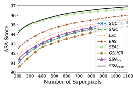
[0pt]      [0pt]

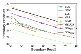
Figure 6: Results on Cityscapes validation. ASA and boundary precision-recall shows that SSN performs favourably against other techniques.

Runtime analysis. We report the approximate runtimes of different techniques, for computing 1000 superpixels on a $512\times 1024$ cityscapes image in Table 1. We compute GPU runtimes using an NVIDIA Tesla V100 GPU. The runtime comparison between SSN_pix and SSN_deep indicates that a significant portion of the SSN computation time is due to the differentiable SLIC. The runtimes indicate that SSN is considerably faster than the implementations of several superpixel algorithms.

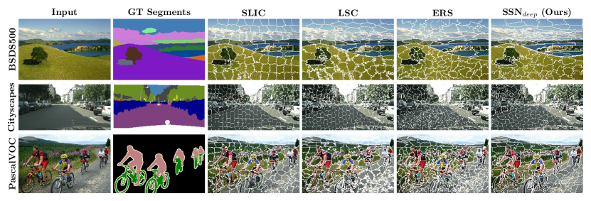
Figure 7: Example visual results on different segmentation benchmarks. Notice the segregation of SSN_deep superpixels around object boundaries.

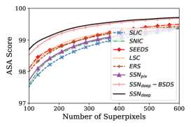
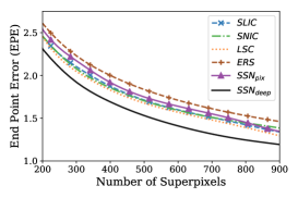
[0pt] (a) VOC Semantic Segmenation      [0pt] (b) MPI-Sintel Optical Flow

Figure 8: Learning task-specific superpixels. (a) ASA scores on PascalVOC2012 validation dataset and (b) EPE scores on Sintel optical flow validation dataset showing the robustness of SSN across different tasks and datasets.

PascalVOC. PascalVOC2012 [11] is another widely-used semantic segmentation benchmark, where we train SSN with 1464 train images and validate on 1449 validation images. Fig. 8(a) shows the ASA scores for different techniques. We do not analyze boundary scores on this dataset as the GT semantic boundaries are dilated with an ignore label. The ASA scores indicate that SSN_deep outperforms other techniques. We also evaluated the BSDS-trained model on this dataset and observed only a marginal drop in accuracy (‘SSN_deep-BSDS’ in Fig. 8(a)). This shows the generalization and robustness of SSN to different datasets. An example visual result is shown in Fig. 7 with more in the supplementary.

Method	IoU
DeepLab [8]	68.9
+ CRF [8]	72.7
+ BI (SLIC) [13]	74.1
+ BI (SSNdeep)	75.3

Table 2: SSN with a downstream CNN. IoU improvements, on the VOC2012 test data, with the integration of SSN into the bilateral inception (BI) network from [13].

We perform an additional experiment where we plug SSN into the downstream semantic segmentation network of [13], The network in [13] has bilateral inception layers that makes use of superpixels for long-range data-adaptive information propagation across intermediate CNN representations. Table 2 shows the Intersection over Union (IoU) score for this joint model evaluated on the test data. The improvements in IoU with respect to original SLIC superpixels used in [13] shows that SSN can also bring performance improvements to the downstream task networks that use superpixels.

5.3 Superpixels for Optical Flow

To demonstrate the applicability of SSN for regression tasks as well, we conduct a proof-of-concept experiment where we learn superpixels that adhere to optical flow boundaries. To this end, we experiment on the MPI-Sintel dataset [7] and use SSN to predict superpixels given a pair of input frames. We use GT optical flow as pixel properties $R$ in the reconstruction loss (Eq. 5) and use L1 loss for $\mathcal{L}$, encouraging SSN to generate superpixels that can effectively represent flow.

The MPI-Sintel dataset consists of 23 video sequences, which we split into disjoint sets of 18 (836 frames) training and 5 (205 frames) validation sequences. To evaluate the superpixels, we follow a similar strategy as for computing ASA. That is, for each pixel inside a superpixel, we assign the average GT optical flow resulting in a segmented flow. Fig. 9 shows sample segmented flows obtained using different types of superpixels. We then compute the Euclidean distance between the GT flow and the segmented flow, which is referred to as end-point error (EPE). The lower the EPE value, the better the superpixels are for representing flow. A sample result in Fig. 9 shows that SSN_deep superpixels are better aligned with the changes in the GT flow than other superpixels. Fig. 8(b) shows the average EPE values for different techniques where SSN_deep performs favourably against existing superpixel techniques. This shows the usefulness of SSN in learning task-specific superpixels.

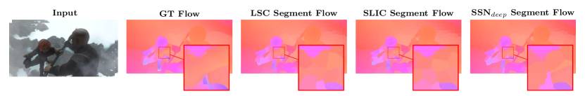
Figure 9: Sample visual result on Sintel optical flow. Segmented flow visuals obtained with different types of superpixels indicate that SSN_deep superpixels can better represent GT optical flow compared to other techniques.

6 Conclusion

We propose a novel superpixel sampling network (SSN) that leverages deep features learned via end-to-end training for estimating task-specific superpixels. To our knowledge, this is the first deep superpixel prediction technique that is end-to-end trainable. Experiments several benchmarks show that SSN consistently performs favorably against state-of-the-art superpixel techniques, while also being faster. Integration of SSN into a semantic segmentation network [13] also results in performance improvements showing the usefulness of SSN in downstream computer vision tasks. SSN is fast, easy to implement, can be easily integrated into other deep networks and has good empirical performance.

SSN has addressed one of the main hurdles for incorporating superpixels into deep networks which is the non-differentiable nature of existing superpixel algorithms. The use of superpixels inside deep networks can have several advantages. Superpixels can reduce the computational complexity, especially when processing high-resolution images. Superpixels can also be used to enforce piece-wise constant assumptions and also help in long-range information propagation [13]. We believe this work opens up new avenues in leveraging superpixels inside deep networks and also inspires new deep learning techniques that use superpixels.

Acknowledgments. We thank Wei-Chih Tu for providing evaluation scripts. We thank Ben Eckart for his help in the supplementary video.

Appendix 0.A Supplementary Material

In Section 0.A.1, we formally define the Acheivable Segmentation Accuracy (ASA) used for evaluating superpixels. Then, in Section 0.A.2, we report F-measure and Compactness scores with more visual results on different datasets. We also include a supplementary video that gives an overview of Superpixel Sampling Networks (SSN) with a glimpse of experimental results.

0.A.1 Evaluation Metrics

Here, we formally define the Achievable Segmentation Accuracy (ASA) metric that is used in the main paper. Given an image $I$ with $n$ pixels, let $H\in\{0,1,\cdots,m\}^{n\times 1}$ denotes the superpixel segmentation with $m$ superpixels. $H$ is composed of $m$ disjoint segments, $H=\bigcup_{j=1}^{m}H^{j}$, where $j^{th}$ segment is represented as $H^{j}$. Similarly, let $G\in\{0,1,\cdots,w\}^{n\times 1}$ denotes ground-truth (GT) segmentation with $w$ segments. $G=\bigcup_{l=1}^{w}G^{l}$, where $G^{l}$ denotes $l^{th}$ GT segment.

ASA Score. The ASA score between a given superpixel segmentation $H$ and the GT segmentation $G$ is defined as

$$ASA(H,G)=\frac{1}{n}\sum_{H^{j}\in S}\max_{G^{l}}|H^{j}\cap G^{l}|,$$ (7)

where $|H^{j}\cap G^{l}|$ denotes the number of overlapping pixels between $S^{j}$ and $G^{l}$. To compute ASA, we first find the GT segment that overlaps the most with each of the superpixel segments and then sum the number of overlapping pixels. As a normalization, we divide the number of overlapping pixels with the number of image pixels $n$. In other words, ASA represents an upper bound on the accuracy achievable by any segmentation step performed on the superpixels.

Boundary Precision-Recall. Boundary Recall (BR) measures how well the boundaries of superpixel segmentation aligns with the GT boundaries. Higher BR score need not correspond to higher quality of superpixels. Superpixels with high BR score can be irregular and may not be useful in practice. Following reviewers’ suggestions, we report Boundary Precision-Recall curves instead of just Boundary Recall scores.

We also report F-measure and Compactness in the next section (Section 0.A.2.1). We use the evaluation scripts from [36] with default parameters to compute Boundary Precision-Recall, F-measure and Compactness.

0.A.2 Additional Experimental Results

0.A.2.1 Compactness and F-measure.

We compute compactness (CO) of different superpixels on the BSDS dataset (Fig. 10(a)). SSN superpixels have only slightly lower CO compared to widely-used SLIC showing the practical utility of SSN. SSN_deep has similar CO as SSN_pix showing that training SSN, while improving ASA and boundary adherence, does not destroy compactness. More importantly, we find SSN to be flexible and responsive to task-specific loss functions and one could use more weight ($\lambda$) for the compactness loss (Eq. 6 in the main paper) if more compact superpixels are desired. In addition, we also plot F-measure scores in Fig. 10(b). In summary, SSN_deep also outperforms other techniques in terms of F-measure while maintaining the compactness as that of SSN_pix. This shows the robustness of SSN with respect to different superpixel aspects.

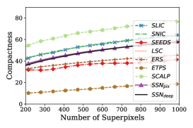
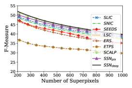
[0pt] (a) Compactness.           [0pt] (b) F-measure.

Figure 10: BSDS500 test results. (a) Compactness and (b) F-measure plots. SSN_deep outperforms other techniques also in terms of F-measure while maintaing the same compactness as that of SSN_pix.

0.A.2.2 Additional visual results.

In this section, we present additional visual results of different techniques and on different datasets. Figs. 11, 12 and 13 show superpixel visual results on three segmentation benchmarks of BSDS500 [4], Cityscapes [10] and PascalVOC [11] respectively. For comparisons, we show the superpixels obtained with 3 existing superpixel techniques of SLIC [1], LSC [25] and ERS [26]. Fig. 14 shows additional visual results on MPI-Sintel [7] where we present sample segmented flows obtained using different types of superpixels.

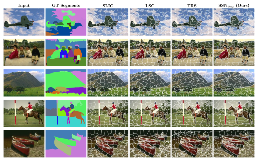
Figure 11: Additional visual results on BSDS500 test images. SSN_deep tends to produce smoother object contours and more superipxels near object boundaries in comparison to other superpixel techniques.

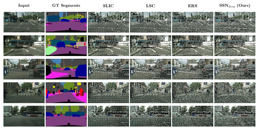
Figure 12: Additional visual results on Cityscapes validation images. SSN_deep tend to generate bigger superpixels on uniform regions (such as road) and more superpixels on smaller objects.

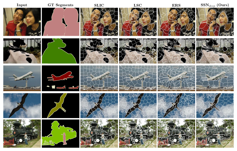
Figure 13: Additional visual results on PascalVOC validation images. SSN_deep tends to produce smoother object contours and more superipxels near object boundaries in comparison to other superpixel techniques.

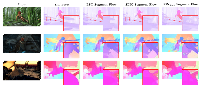
Figure 14: Additional visual results on Sintel images. Segmented flow visuals obtained with different types of superpixels indicate that SSN_deep superpixels can better represent GT optical flow compared to other techniques.

References

- [1] Achanta, R., Shaji, A., Smith, K., Lucchi, A., Fua, P., Süsstrunk, S.: SLIC superpixels compared to state-of-the-art superpixel methods. IEEE Transactions on Pattern Analysis and Machine Intelligence (TPAMI) 34(11), 2274–2282 (2012)
- [2] Achanta, R., Susstrunk, S.: Superpixels and polygons using simple non-iterative clustering. In: IEEE Conference on Computer Vision and Pattern Recognition (CVPR) (2017)
- [3] Aljalbout, E., Golkov, V., Siddiqui, Y., Cremers, D.: Clustering with deep learning: Taxonomy and new methods. arXiv preprint arXiv:1801.07648 (2018)
- [4] Arbelaez, P., Maire, M., Fowlkes, C., Malik, J.: Contour detection and hierarchical image segmentation. IEEE Transactions on Pattern Analysis and Machine Intelligence (TPAMI) 33(5), 898–916 (2011)
- [5] Van den Bergh, M., Boix, X., Roig, G., Van Gool, L.: SEEDS: Superpixels extracted via energy-driven sampling. International Journal of Computer Vision (IJCV) 111(3), 298–314 (2015)
- [6] Van den Bergh, M., Carton, D., Van Gool, L.: Depth SEEDS: Recovering incomplete depth data using superpixels. In: IEEE Workshop on Applications of Computer Vision (WACV). pp. 363–368 (2013)
- [7] Butler, D.J., Wulff, J., Stanley, G.B., Black, M.J.: A naturalistic open source movie for optical flow evaluation. In: European Conference on Computer Vision (ECCV). pp. 611–625. Springer (2012)
- [8] Chen, L.C., Papandreou, G., Kokkinos, I., Murphy, K., Yuille, A.L.: Semantic image segmentation with deep convolutional nets and fully connected CRFs. In: International Conference on Learning Representations (ICLR) (2015)
- [9] Comaniciu, D., Meer, P.: Mean shift: A robust approach toward feature space analysis. IEEE Transactions on Pattern Analysis and Machine Intelligence (TPAMI) 24(5), 603–619 (2002)
- [10] Cordts, M., Omran, M., Ramos, S., Rehfeld, T., Enzweiler, M., Benenson, R., Franke, U., Roth, S., Schiele, B.: The cityscapes dataset for semantic urban scene understanding. In: IEEE Conference on Computer Vision and Pattern Recognition (CVPR) (2016)
- [11] Everingham, M., Eslami, S.A., Van Gool, L., Williams, C.K., Winn, J., Zisserman, A.: The Pascal visual object classes challenge: A retrospective. International Journal of Computer Vision (IJCV) 111(1), 98–136 (2015)
- [12] Felzenszwalb, P.F., Huttenlocher, D.P.: Efficient graph-based image segmentation. International Journal of Computer Vision (IJCV) (2004)
- [13] Gadde, R., Jampani, V., Kiefel, M., Kappler, D., Gehler, P.: Superpixel convolutional networks using bilateral inceptions. In: European Conference on Computer Vision (ECCV) (2016)
- [14] Giraud, R., Ta, V.T., Papadakis, N.: SCALP: Superpixels with contour adherence using linear path. In: International Conference on Pattern Recognition (ICPR) (2016)
- [15] Gould, S., Rodgers, J., Cohen, D., Elidan, G., Koller, D.: Multi-class segmentation with relative location prior. International Journal of Computer Vision 80(3), 300–316 (2008)
- [16] Greff, K., Rasmus, A., Berglund, M., Hao, T., Valpola, H., Schmidhuber, J.: Tagger: Deep unsupervised perceptual grouping. In: Advances in Neural Information Processing Systems (NIPS) (2016)
- [17] Greff, K., van Steenkiste, S., Schmidhuber, J.: Neural expectation maximization. In: Advances in Neural Information Processing Systems (NIPS) (2017)
- [18] He, S., Lau, R.W., Liu, W., Huang, Z., Yang, Q.: SuperCNN: A superpixelwise convolutional neural network for salient object detection. International Journal of Computer Vision (IJCV) 115(3), 330–344 (2015)
- [19] Hershey, J.R., Chen, Z., Le Roux, J., Watanabe, S.: Deep clustering: Discriminative embeddings for segmentation and separation. In: IEEE International Conference on Acoustics, Speech and Signal Processing (ICASSP) (2016)
- [20] Hu, Y., Song, R., Li, Y., Rao, P., Wang, Y.: Highly accurate optical flow estimation on superpixel tree. Image and Vision Computing 52, 167–177 (2016)
- [21] Ioffe, S., Szegedy, C.: Batch normalization: Accelerating deep network training by reducing internal covariate shift. In: International Conference on Machine Learning (ICML). pp. 448–456 (2015)
- [22] Jia, Y., Shelhamer, E., Donahue, J., Karayev, S., Long, J., Girshick, R., Guadarrama, S., Darrell, T.: Caffe: Convolutional architecture for fast feature embedding. In: ACM Multimedia (MM). pp. 675–678 (2014)
- [23] Kingma, D.P., Ba, J.: Adam: A method for stochastic optimization. In: International Conference on Learning Representations (ICLR) (2015)
- [24] Levinshtein, A., Stere, A., Kutulakos, K.N., Fleet, D.J., Dickinson, S.J., Siddiqi, K.: Turbopixels: Fast superpixels using geometric flows. IEEE Transactions on Pattern Analysis and Machine Intelligence (TPAMI) 31(12), 2290–2297 (2009)
- [25] Li, Z., Chen, J.: Superpixel segmentation using linear spectral clustering. In: IEEE Conference on Computer Vision and Pattern Recognition (CVPR) (2015)
- [26] Liu, M.Y., Tuzel, O., Ramalingam, S., Chellappa, R.: Entropy rate superpixel segmentation. In: IEEE Conference on Computer Vision and Pattern Recognition (CVPR) (2011)
- [27] Liu, Y.J., Yu, C.C., Yu, M.J., He, Y.: Manifold slic: A fast method to compute content-sensitive superpixels. In: IEEE Conference on Computer Vision and Pattern Recognition (CVPR) (2016)
- [28] Lu, J., Yang, H., Min, D., Do, M.N.: Patch match filter: Efficient edge-aware filtering meets randomized search for fast correspondence field estimation. In: IEEE Conference on Computer Vision and Pattern Recognition (CVPR). pp. 1854–1861 (2013)
- [29] Machairas, V., Faessel, M., Cárdenas-Peña, D., Chabardes, T., Walter, T., Decencière, E.: Waterpixels. IEEE Transactions on Image Processing (TIP) 24(11), 3707–3716 (2015)
- [30] Perazzi, F., Krähenbühl, P., Pritch, Y., Hornung, A.: Saliency filters: Contrast based filtering for salient region detection. In: IEEE Conference on Computer Vision and Pattern Recognition (CVPR). pp. 733–740 (2012)
- [31] Rasmus, A., Berglund, M., Honkala, M., Valpola, H., Raiko, T.: Semi-supervised learning with ladder networks. In: Advances in Neural Information Processing Systems (NIPS) (2015)
- [32] Ren, C.Y., Prisacariu, V.A., Reid, I.D.: gSLICr: SLIC superpixels at over 250hz. arXiv preprint arXiv:1509.04232 (2015)
- [33] Ren, X., Malik, J.: Learning a classification model for segmentation. In: IEEE Conference on Computer Vision and Pattern Recognition (CVPR) (2003)
- [34] Sharma, A., Tuzel, O., Liu, M.Y.: Recursive context propagation network for semantic scene labeling. In: Advances in Neural Information Processing Systems (NIPS) (2014)
- [35] Shu, G., Dehghan, A., Shah, M.: Improving an object detector and extracting regions using superpixels. In: IEEE Conference on Computer Vision and Pattern Recognition (CVPR). pp. 3721–3727 (2013)
- [36] Stutz, D., Hermans, A., Leibe, B.: Superpixels: An evaluation of the state-of-the-art. Computer Vision and Image Understanding 166(C), 1–27 (2018)
- [37] Sun, D., Liu, C., Pfister, H.: Local layering for joint motion estimation and occlusion detection. In: Proceedings of the IEEE Conference on Computer Vision and Pattern Recognition. pp. 1098–1105 (2014)
- [38] Tu, W.C., Liu, M.Y., Jampani, V., Sun, D., Chien, S.Y., Yang, M.H., Kautz, J.: Learning superpixels with segmentation-aware affinity loss. In: IEEE Conference on Computer Vision and Pattern Recognition (CVPR) (2018)
- [39] Veksler, O., Boykov, Y., Mehrani, P.: Superpixels and supervoxels in an energy optimization framework. In: European Conference on Computer Vision (ECCV) (2010)
- [40] Xie, J., Girshick, R., Farhadi, A.: Unsupervised deep embedding for clustering analysis. In: International conference on machine learning (ICML) (2016)
- [41] Yamaguchi, K., McAllester, D., Urtasun, R.: Robust monocular epipolar flow estimation. In: IEEE Conference on Computer Vision and Pattern Recognition (CVPR). pp. 1862–1869 (2013)
- [42] Yan, J., Yu, Y., Zhu, X., Lei, Z., Li, S.Z.: Object detection by labeling superpixels. In: IEEE Conference on Computer Vision and Pattern Recognition (CVPR). pp. 5107–5116 (2015)
- [43] Yang, C., Zhang, L., Lu, H., Ruan, X., Yang, M.H.: Saliency detection via graph-based manifold ranking. In: IEEE Conference on Computer Vision and Pattern Recognition (CVPR) (2013)
- [44] Yang, F., Lu, H., Yang, M.H.: Robust superpixel tracking. IEEE Transactions on Image Processing 23(4), 1639–1651 (2014)
- [45] Yao, J., Boben, M., Fidler, S., Urtasun, R.: Real-time coarse-to-fine topologically preserving segmentation. In: IEEE Conference on Computer Vision and Pattern Recognition (CVPR) (2015)
- [46] Zhu, W., Liang, S., Wei, Y., Sun, J.: Saliency optimization from robust background detection. In: IEEE Conference on Computer Vision and Pattern Recognition (CVPR) (2014)