A Common Source for Scalars:
Axiflavon-Higgs Unification

Abstract

We propose a unified model of scalar particles that addresses the flavour hierarchies, solves the strong CP problem, delivers a dark matter candidate, and provides the trigger for electroweak symmetry breaking. Besides furnishing a unification of the recently proposed axiflavon with a Goldstone-Higgs sector, the scenario can also be seen as adding a model of flavour (and strong CP conservation along with axion dark matter) to elementary Goldstone-Higgs setups. In particular, we derive bounds on the axion decay constant from the need to generate a SM-like Higgs potential at low energies, which we confront with constraints from flavour physics and cosmology. In the minimal implementation, we find that the axion decay constant is restricted to a thin stripe of $f_{a}\approx(10^{11}-10^{12})\,\text{GeV}$, while adding right-handed neutrinos allows to realize a heavy-axion model at lower energies, down to $f_{a}\sim 10$ TeV.

I Introduction

Although the Standard Model (SM) of particle physics provides an excellent description of nature around the weak scale, it has several shortcomings that lead us to the conclusion that it is rather an effective low-energy parametrization of a more fundamental theory of nature.

Amongst the most pressing issues are the missing candidate to generate the dark matter populating our universe, and the failure to explain large hierarchies present in the fermion masses and mixings. Beyond that, the apparent conservation of CP symmetry in strong interactions is in tension with in principle unsuppressed sources of CP violation in the QCD Lagrangian. Finally, although the SM provides a successful parameterization of electroweak symmetry breaking (EWSB) via the Higgs mechanism, the origin of the Higgs potential is unknown.

The flavour hierarchies in the SM can be addressed via the Froggatt–Nielsen (FN) mechanism Froggatt and Nielsen (1979), i.e. by chirally charging the SM fermions under a $\mathrm{U}(1)_{\mathrm{H}}$ flavour symmetry controlling their masses and mixings. For the FN mechanism to work, the field content of the SM has to be augmented (at least) by a complex scalar field, $\Phi$, spontaneously breaking the $\mathrm{U}(1)_{\mathrm{H}}$, and vector-like fermions, $\xi_{j}$, dubbed the FN messengers, which connect the different SM-fermion chiralities, bridging their $\mathrm{U}(1)_{\mathrm{H}}$ charge difference via a chain of $\Phi$ insertions. Taking the FN messengers to reside much above the electroweak (EW) scale, they can be integrated out in the IR description. Then, once the $\mathrm{U}(1)_{\mathrm{H}}$ is spontaneously broken by $\langle\Phi\rangle\neq 0$, the SM Yukawa couplings are effectively reproduced starting with $\mathcal{O}(1)$ couplings in the UV theory.

As shown in a previous work Calibbi et al. (2017) (see also Ref. Ema et al. (2017)), the angular component of $\Phi$, which plays no vital role in the original FN mechanism, can be identified with the QCD axion Peccei and Quinn (1977); Wilczek (1978); Weinberg (1978); Kim (1979); Shifman et al. (1980); Dine et al. (1981); Zhitnitsky (1980), thereby addressing two more issues of the SM, namely the strong CP problem and the DM puzzle Preskill et al. (1983); Abbott and Sikivie (1983); Dine and Fischler (1983), in a unified scenario. In particular, as the axion couplings are now dictated by the flavour structure, the predictivity of the model is increased.

In this paper, we take a further step to unify the scalar degrees of freedom in the theory by combining the axiflavon field, $\Phi$, and the Higgs boson such that the flavour, strong CP, and DM problems remain solved, while successfully triggering EWSB. We thus embed the Higgs, the axion, and the flavon in a single multiplet, $\Sigma$, transforming under the enlarged symmetry group $\mathcal{G}\supset\mathrm{U}(1)_{\mathrm{H}}\times G_{\text{EW}}$, with $G_{\text{EW}}\equiv\mathrm{SU}(2)_{\mathrm{L}}\times\mathrm{U}(1)_{Y}$. Within the FN setup, the flavon mass and the Higgs mass are hierarchically different. In the unified picture, this very fact suggests that both the axion and the Higgs boson components should correspond to pseudo-Nambu–Goldstone bosons (pNGBs), providing an example of axion-Higgs unification Redi and Strumia (2012) and allowing for dynamical EWSB via the Coleman-Weinberg potential for the emerging Goldstone Higgs. Interestingly, the vanishing of the quartic Higgs coupling in the SM around $10^{10}$ GeV, just about at the natural scale for axiflavon dark matter, might hint both to Goldstone nature of the Higgs and to a connection between these two scalar sectors.

From a different perspective, the proposed model can be seen as adding a flavour story to the recently proposed elementary-Goldstone-Higgs scenario Alanne et al. (2015, 2016). Including the axiflavon can address fermion masses and mixings in these models, while providing a solution to the strong CP problem. This is a compelling renormalizable alternative to partial compositeness Kaplan (1991) generating flavour hierarchies in composite-Higgs models. Furthermore, in this way the flavour structure can be achieved without the need of adding a new disconnected scalar or a new symmetry-breaking mechanism. We stress that the fine-tuning problem affecting the EW scale in this setup is not worse than the one in the usual FN mechanism, which already involves the tuning of the Higgs portal coupling $\lambda|H|^{2}|\Phi|^{2}$. At the end of the paper, we also comment on the option to realize the model around the TeV scale.

Before working out the setup and its predictions in detail, we summarize the main model building steps. We formulate the theory at the scale $f$ as a linear sigma model for the field $\Sigma$. Yukawa interactions between $\Sigma$ and the FN messengers are introduced as a microscopic realization of the FN mechanism, and similarly for the SM fields. The global symmetry breaking pattern is $\mathcal{G}\xrightarrow{\text{\tiny$\langle\Sigma\rangle$}}\mathcal{H}\supset G_{\text{EW}}$, with the axion and the Higgs residing in the $\mathcal{G}/\mathcal{H}$ coset. Notice that $\mathcal{H}$ may or may not contain custodial protection, as the scale $f$ is by construction much larger than the Higgs vacuum expectation value, so that the custodial-breaking effects are strongly suppressed. The simplest choice for $\mathcal{G}$ is to keep the flavour symmetry as an abelian factor, $\mathcal{G}=\mathcal{G^{\prime}}\times\mathrm{U}(1)_{\mathrm{H}}$. The minimal choice for $\mathcal{G^{\prime}}$ is based on $\mathrm{SU}(3)$ and the next-to-minimal on $\mathrm{SO}(5)$ Agashe et al. (2005). Both result in a similar structure, and in the following we focus only on the latter. Finally, we assume that the explicit breaking of $\mathcal{G}$ originates from the SM sector only, namely from the QCD anomaly, EW gauging, and via the SM fermions coming as $\mathcal{G}$ spurions. Conversely, the FN messengers always enter as full representations.

This article is organized as follows. In Section II, we detail the setup and main features of the model, including the structure of the linear sigma model and the generation of mass hierarchies via the FN mechanism. Section III contains the calculation and analysis of the Higgs potential, which leads to a prediction for the axion decay constant. Here, we also discuss the impact of including right-handed neutrinos into the setup and potential constraints from flavour physics and cosmology. Finally, Section IV contains our conclusions. In two appendices we discuss the assumptions regarding the mass spectrum of the FN messengers as well as the contributions from light fermions to the Higgs potential.

II Model Setup

In the following, we present the explicit model setup. The symmetry-breaking pattern that leads to the unified realization of the Higgs doublet and the axion as pNGBs reads

$$\left[\mathrm{SO}(5)\times\mathrm{U}(1)_{\mathrm{H}}\right]\times\mathrm{U}(1)_{X}\rightarrow\mathrm{SO}(4)\times\mathrm{U}(1)_{X}\,,$$ (1)

where the $\mathrm{U}(1)_{X}$ factor is introduced to reproduce the fermion hypercharges. The pattern of Eq. (1) is obtained within a linear $\sigma$-model for the field $\Sigma$ living in the fundamental representation, $\mathbf{5}$, of $\mathrm{SO}(5)$ and having $\mathrm{U}(1)_{\mathrm{H}}$ flavour charge $H_{\Sigma}=1$, with the potential

$$V(\Sigma,\Sigma^{*})=\lambda_{1}\left(\Sigma^{\dagger}\Sigma\right)^{2}-\lambda_{2}\,\Sigma^{T}\Sigma\,\Sigma^{\dagger}\Sigma^{*}-\mu^{2}\Sigma^{\dagger}\Sigma\,.$$ (2)

The EW gauge group is embedded in $\mathrm{SO}(5)$ by defining the usual $\mathrm{SU}(2)_{\mathrm{L}}\times\mathrm{SU}(2)_{\mathrm{R}}\cong\mathrm{SO}(4)$ generators:

$$T_{ij}^{a\,\mathrm{L,R}}=-\frac{i}{2}\left[\frac{1}{2}\epsilon^{abc}(\delta^{b}_{i}\delta^{c}_{j}-\delta^{c}_{i}\delta^{b}_{j})\pm(\delta_{i}^{a}\delta_{j}^{4}-\delta_{j}^{a}\delta_{i}^{4})\right].$$ (3)

The $\mathrm{SO}(4)$-preserving minimum is then given by $\langle\Sigma\rangle=(0,0,0,0,f/\sqrt{2})$, with $\mu^{2}=(\lambda_{1}-\lambda_{2})f^{2}$, and after the breaking, Eq. (1), the scalar sector can be parametrized as

$$\Sigma=e^{i(\sqrt{2}h_{\hat{a}}\hat{T}^{\hat{a}}+a)/f}\begin{pmatrix}\widetilde{H}\\ (f+\sigma)/\sqrt{2}\end{pmatrix}\,,$$ (4)

where the broken generators, $\hat{T}^{\hat{a}}$, are given by

$$\hat{T}_{ij}^{\hat{a}}=-\frac{i}{\sqrt{2}}\left[\delta_{i}^{\hat{a}}\delta_{j}^{5}-\delta_{j}^{\hat{a}}\delta_{i}^{5}\right].$$ (5)

As physical states, one finds a heavy Higgs doublet, $\widetilde{H}$, with mass $m^{2}_{\tilde{H}}=2\lambda_{2}f^{2}$, and a heavy flavon, $\sigma$, with mass $m^{2}_{\sigma}=2(\lambda_{1}-\lambda_{2})f^{2}$, while the SM-like Higgs doublet, $h_{\hat{a}}$, and the axion, $a$, are instead pNGBs. The potential is bounded from below if $\lambda_{1}>\lambda_{2}>0$.

The FN messengers are denoted by $\xi_{j}$, where the subscript refers to the $\mathrm{U}(1)_{\mathrm{H}}$ charge, $H_{\xi_{j}}=j$. Each of them transforms in the spinorial representation, $\mathbf{4}$, of $\mathrm{SO}(5)$ and is vectorial under $\mathrm{SO}(5)\times\mathrm{U}(1)_{\mathrm{H}}$.

Similarly, the SM fermions, $q_{\mathrm{L}}^{i}$, $u_{\mathrm{R}}^{i}$, and $d_{\mathrm{R}}^{i}$ (with $i=1,2,3$ a flavour index), are introduced as spurions, $\Psi_{f}^{i}$, in the spinorial representation:

$$\Psi^{i}_{q_{\mathrm{L}}}=\Delta_{\mathrm{L}}^{T}q^{i}_{\mathrm{L}},\quad\Psi^{i}_{u_{\mathrm{R}}}=\Delta_{u}^{T}u^{i}_{\mathrm{R}},\quad\Psi^{i}_{d_{\mathrm{R}}}=\Delta_{d}^{T}d_{\mathrm{R}}^{i},$$ (6)

where

$$\begin{split}\Delta_{\mathrm{L}}&=\left(\begin{array}[]{cccc}1&0&0&0\\ 0&1&0&0\\ \end{array}\right),\\ \Delta_{u}&=\left(0,0,1,0\right),\quad\Delta_{d}=\left(0,0,0,1\right).\end{split}$$ (7)

The $\mathrm{U}(1)_{\mathrm{H}}$ charge of each $\Psi^{i}_{f}$ is chosen such that the correct pattern of masses and mixings is reproduced. The larger the charge difference between the left- and right-handed components of a given fermion, the more suppressed is the resulting mass term. Notice that the $\Psi$-fields have to be considered only as $\mathrm{SO}(5)$ spurions, while the $\mathrm{U}(1)_{\mathrm{H}}$ needs to be exact at the Lagrangian level. For both the SM fermions and the FN messengers, the $\mathrm{U}(1)_{X}$ charge is chosen to match the correct hypercharge, $Y=T_{3}+X$, and will be omitted in the following.

The Lagrangian of the system includes renormalizable operators made out of $\Psi_{f}^{i}$, $\xi_{j}$, and $\Sigma$ allowed by symmetries:

$$\begin{split}-\mathcal{L}\,&=\,\sum_{j}\left(a_{j}\bar{\xi}_{j+1}\,\Gamma^{\alpha}\,\Sigma_{\alpha}\,\xi_{j}+\text{h.c.}\right)+m_{j}\,\bar{\xi}_{j}\,\xi_{j},\\ &+\sum_{i,f}z_{i}^{f}\,\bar{\Psi}^{i}_{f}\,\Gamma^{\alpha}\,\Sigma_{\alpha}\,\xi_{j}+\tilde{z}_{i}^{f}\,\bar{\xi}_{j+2}\,\Gamma^{\alpha}\,\Sigma_{\alpha}\,\Psi^{i}_{f}+\text{h.c.}\\ &+x\,\bar{\Psi}^{3}_{q_{L}}\,\Gamma^{\alpha}\,\Sigma_{\alpha}\,\Psi^{3}_{u_{R}}+\text{h.c.}\,,\end{split}$$ (8)

where $\Gamma^{a}$ are the matrices defining the spinorial representation. In the Lagrangian above, the first line contains the interactions of the FN messengers with the $\Sigma$-field and their (vector-like) mass terms, while the second line consists of Yukawa couplings involving the SM fermions and the FN messengers, where $f=q_{\mathrm{L}},u_{\mathrm{R}},d_{\mathrm{R}}$, and $j\equiv j(f,i)=H_{f^{i}}-1$ is such that the terms are $\mathrm{U}(1)_{\mathrm{H}}$ invariant. Notice that the use of the spinorial representation is particularly suitable for the purpose of building the FN chain: both $\xi$-fields appear symmetrically in the Yukawa coupling and thus only a single species of heavy fermions is needed. Finally, the last line accounts for the fact that the top mass features no suppression, and thus a direct coupling of $t_{\mathrm{L}}$ and $t_{\mathrm{R}}$ via the $\Sigma$-field must be allowed.

Before presenting the computation of the Higgs potential, let us discuss an example to show how the FN mechanism is explicitly realized in our setup.

II.1 Mass hierarchies from broken $\mathrm{U}(1)_{\mathrm{H}}$

Consider two chiral fermions, $\Psi_{q_{\mathrm{L}}}^{3}$ and $\Psi_{u_{\mathrm{R}}}^{2}$ for concreteness, as given in Eq. (6), and two FN messengers, $\xi_{2,3}$, with the mass-mixing Lagrangian

$$\begin{split}-\mathcal{L}\supset&\,z\,\bar{\Psi}_{u_{\mathrm{R}}}^{2}\Sigma^{\prime}\xi_{3}+\tilde{z}\,\bar{\xi}_{2}\Sigma^{\prime}\Psi_{q_{\mathrm{L}}}^{3}+a_{2}\,\bar{\xi}_{3}\Sigma^{\prime}\xi_{2}+\text{h.c.}\\ &+m\left(\bar{\xi}_{2}\xi_{2}+\bar{\xi}_{3}\xi_{3}\right),\end{split}$$ (9)

where we have defined $\Sigma^{\prime}\equiv\Gamma^{\alpha}\,\Sigma_{\alpha}$. The Lagrangian above corresponds to the flavour charges $H_{q_{\mathrm{L}}^{3}}=1$ and $H_{u_{\mathrm{R}}^{2}}=4$ and, as we shall see, reproduces the term in Eq. (56) for the $t_{\rm L}$-$c_{\rm R}$ mixing. All dimensionless couplings are assumed to be $z\sim\tilde{z}\sim a_{2}\sim\mathcal{O}(1)$.

By integrating out $\xi_{2}$ and $\xi_{3}$ at the tree level, one finds the effective Lagrangian, $\mathcal{L}_{\text{eff}}$, which, at the leading order in $1/m$, reads

$$-\mathcal{L_{\text{eff}}}=z\,\tilde{z}\,a_{2}\,\frac{1}{m^{2}}\bar{\Psi}_{u_{\mathrm{R}}}^{2}\Sigma^{\prime}\Sigma^{\prime}\Sigma^{\prime}\Psi_{q_{\mathrm{L}}}^{3}+\text{h.c.}$$ (10)

Below the symmetry-breaking scale and after integrating out the flavon and the second Higgs doublet, the $\Sigma$-field can be written by the Goldstone parametrization in the unitary gauge as

$$\Sigma=\frac{f}{\sqrt{2}}\,e^{ia/f}\left(0,0,\text{sin}\,h/f,0,\text{cos}\,h/f\right)^{T},$$ (11)

where $h$ represents the Higgs field, and $a$ is the axion. Using Eq. (11), we can single out the contribution to the mass matrix in Eq. (10):

$$-\mathcal{L_{\text{eff}}}\supset m_{32}\bar{c}_{\rm R}t_{\rm L}+\text{h.c.}\,,$$ (12)

$$m_{32}=\frac{1}{\sqrt{2}}z\,\tilde{z}\,a_{2}\frac{f^{2}}{2m^{2}}f\,\text{sin}(\langle h\rangle/f)+\dots\,,$$ (13)

where $f\,\sin(\langle h\rangle/f)\equiv v$ is to be identified with the EW scale and the dots stand for higher orders in $f^{2}/2m^{2}$. Defining $\delta_{ij}\equiv H_{q_{\mathrm{L}}^{i}}-H_{q_{\mathrm{R}}^{j}}$, we see that the suppression with respect to the top mass is $m_{ij}/m_{t}\sim\left(f/\sqrt{2}m\right)^{|\delta_{ij}|-1}$ with $\delta_{32}=3$ in the present case. The addtional $-1$ in the exponent, which is not present in the usual FN setup, compensates for the Higgs carrying one unit of flavour charge, since it is unified in the $\Sigma$-field.

One can show that this result holds in general for odd $|\delta_{ij}|$, while for even $|\delta_{ij}|$ the corresponding term vanishes due to the properties of the $\Gamma$ matrices; see footnote 1. We thus conclude that a general entry in the fermion mass matrix, $m_{ij}$, corresponding to a charge difference of $|\delta_{ij}|$ is suppressed with respect to the top mass by

$$\frac{m_{ij}}{m_{t}}\sim\left(\frac{f^{2}}{2m^{2}}\right)^{\frac{|\delta_{ij}|-1}{2}}\,,\quad|\delta_{ij}|\,\text{odd}\,.$$ (14)

Eq. (14) shows that $\left(f^{2}/2m^{2}\right)\equiv\epsilon$ is the smallest building block we can use to reproduce the flavour hierarchies, and therefore we identify $\epsilon=\text{sin}\,\theta_{\mathrm{C}}\simeq 0.23$ with $\theta_{\mathrm{C}}$ being the Cabibbo angle. As a final check, for the $t_{\rm L}$-$c_{\rm R}$ mixing with $\delta_{32}=3$, we see that Eq. (14) gives the correct entry $n_{32}=1$ in Eq. (57).

III Higgs Potential and Constraints on the Axion Decay Constant

In this section, we compute the Higgs potential generated by the interaction with the top quark and the FN messengers which directly couple to it. A charge assignment that is compatible with the top mass must satisfy $|\delta_{33}|\equiv|H_{q_{\rm L}^{3}}-H_{u_{\rm R}^{3}}|=1$, and we take $H_{q_{\rm L}^{3}}=1$, and $H_{u_{\rm R}^{3}}=2$. This corresponds to

$$\begin{split}-\mathcal{L}\supset&\left(a_{0}e^{i\alpha}\bar{\xi}_{1}\Sigma^{\prime}\xi_{0}+\text{h.c.}\right)\,+m(\bar{\xi_{0}}\xi_{0}+\bar{\xi}_{1}\xi_{1})\\[2.84526pt] &+\left(xe^{i\zeta}\bar{\Psi}^{3}_{q_{\rm L}}\Sigma^{\prime}\Psi^{3}_{u_{\rm R}}+z_{\rm L}e^{i\zeta_{\rm L}}\bar{\Psi}^{3}_{q_{\rm L}}\Sigma^{\prime}\xi_{0}\right.\\ &\left.\quad+z_{\rm R}e^{i\zeta_{\rm R}}\bar{\Psi}^{3}_{u_{\rm R}}\Sigma^{\prime}\xi_{1}+\text{h.c.}\right)\,,\end{split}$$ (15)

where $z_{\mathrm{L,R}}\equiv z_{3}^{q_{\mathrm{L}},u_{\mathrm{R}}}$ and potential phases have been pulled out into $\zeta_{\mathrm{L,R}}$. Note that we are here assuming mass degeneracy for the messenger fields, $m_{0}=m_{1}\equiv m$, and we are setting to zero interactions involving other FN messengers which have to be there to reproduce the correct mixings (e.g., the $\bar{\xi}_{2}\Sigma^{\prime}\Psi_{q_{\rm L}}^{3}$ term in Eq. (9)) but do not alter the conclusion of this section. We comment on breaking the mass degeneracy in Appendix A, while the contribution to the Higgs potential from sectors involving lighter fermions is discussed in Appendix B.

Let us first compute the top mass according to Eq. (15) in the background of $h$. This can be done by solving the characteristic polynomial for the fermion mass matrix, or alternatively by integrating out the heavy fields at the tree level. The expression for $m_{t}$ is obtained as an expansion in $f^{2}/2m^{2}$ and $h/f$:

$$\begin{split}m_{t}^{2}(h)=&\left(\alpha_{0}-\alpha_{2}\frac{f^{2}}{2m^{2}}-\alpha_{4}\frac{f^{4}}{4m^{4}}\right)\frac{f^{2}}{2}\text{sin}^{2}(h/f)\\ &-\beta_{4}\frac{f^{4}}{4m^{4}}\frac{f^{2}}{2}\text{sin}^{4}(h/f)+\text{h.o.},\end{split}$$ (16)

where h.o. stands for higher-order contributions in $f^{2}/2m^{2}$ and $(h/f)^{n}$ terms with $n\geq 6$, and

$$\begin{split}\alpha_{0}=&\,x^{2},\\ \alpha_{2}=&\,x^{2}\,\left(z_{\mathrm{L}}^{2}+z_{\mathrm{R}}^{2}\right)-2\,x\,z_{\mathrm{L}}\,z_{\mathrm{R}}\,a_{0}\,\cos\,\Omega,\\ \alpha_{4}=&-x^{2}\,\left(z_{\mathrm{L}}^{4}+z_{\mathrm{L}}^{2}z_{\mathrm{R}}^{2}+z_{\mathrm{R}}^{4}\right)\\ &+a_{0}^{2}\left(3x^{2}z_{\mathrm{L}}^{2}+z_{\mathrm{R}}^{2}(3x^{2}-z_{\mathrm{L}}^{2})\right)\\ &-2a_{0}xz_{\mathrm{L}}z_{\mathrm{R}}\left(a_{0}^{2}-z_{\mathrm{L}}^{2}-z_{\mathrm{R}}^{2}\right)\cos\,\Omega,\\ \beta_{4}=&\,x^{4}\left(z_{\mathrm{L}}^{2}+z_{\mathrm{R}}^{2}\right)-6x^{3}\,z_{\mathrm{L}}\,z_{\mathrm{R}}\,a_{0}\,\cos\,\Omega,\end{split}$$ (17)

with $\Omega\equiv\alpha-\zeta_{\mathrm{L}}+\zeta-\zeta_{\mathrm{R}}$. The expression of Eq. (16) needs to coincide with the SM result, $m_{t}^{2}=\frac{1}{2}y_{t}^{2}h^{2}$ implying $y_{t}\simeq x$ at the leading order.

We compute the Higgs potential by matching the SM effective potential renormalized at the scale $m$ (where the new physics kicks in) with the one in the axiflavon-Higgs scenario. We work out the one-loop matching explicitly in the following. The SM effective potential up to one-loop level, keeping only the top contribution, reads

$$\begin{split}V_{\text{SM}}^{(1)}=&\frac{1}{4}\lambda(m)h^{4}-\frac{1}{2}\mu^{2}(m)h^{2}\\ &-\frac{N_{c}}{16\pi^{2}}m_{t}^{4}(h)\left(\log\frac{m^{2}_{t}(h)}{m^{2}}-\frac{3}{2}\right),\end{split}$$ (18)

where $N_{c}=3$, and all the couplings are evaluated at the scale $m$, including $y_{t}(m)$ within $m_{t}(h)$.

In the axiflavon-Higgs picture, the Higgs potential arises at the loop level, and it is given in terms of the field-dependent masses of the physical eigenstates, namely the SM particles and the FN messengers. Considering only the top sector in Eq. (15) yields

$$\begin{split}V_{\text{AFH}}^{(1)}=&-\frac{N_{c}}{16\pi^{2}}\left\{m_{t}^{4}(h)\left(\log\frac{m^{2}_{t}(h)}{m^{2}}-\frac{3}{2}\right)\right.\\ &\qquad\ \ \left.+\sum_{j}m_{\xi_{j}}^{4}(h)\left(\log\frac{m^{2}_{\xi_{j}}(h)}{m^{2}}-\frac{3}{2}\right)\right\}.\end{split}$$ (19)

Then, by requiring

$$V_{\text{SM}}^{(1)}=V_{\text{AFH}}^{(1)},$$ (20)

we obtain

$$\begin{split}V_{4}\equiv&\frac{1}{4}\lambda(m)h^{4}-\frac{1}{2}\mu^{2}(m)h^{2}\\ =&-\frac{N_{c}}{16\pi^{2}}\sum_{j}m_{\xi_{j}}^{4}(h)\left(\log\frac{m^{2}_{\xi_{j}}(h)}{m^{2}}-\frac{3}{2}\right)\,.\end{split}$$ (21)

A few comments are in order: the contribution from the top eigenstate appears on both side of Eq. (20), and therefore it cancels. Such cancelation takes care of the large logarithm arising from the hierarchy between the EW and the flavon scale. We expect this behaviour to persist beyond the one-loop level, given that the pure SM contribution always appears on both sides, so that Eq. (21) gives the leading-order matching condition.

To compute the RHS of Eq. (21), we parametrize the field-dependent FN masses as

$$m_{\xi_{j}}^{2}(h)=m^{2}+f_{j}(h),$$ (22)

where $f_{j}(h)\sim f\times m$. By expanding the logarithm, we see that

$$\begin{split}V_{4}=-\frac{N_{c}}{16\pi^{2}}\sum_{j}&\left[-2f_{j}(h)m^{2}+\frac{f_{j}^{3}(h)}{3m^{2}}-\frac{f_{j}^{4}(h)}{12m^{4}}\right.\\ &\left.\ +\frac{f_{j}^{5}(h)}{30m^{6}}-\frac{f_{j}^{6}(h)}{60m^{8}}+\text{h.o.}\right],\end{split}$$ (23)

where we dropped a constant term. The computation of $F_{n}=\sum_{j}f_{j}^{n}(h)$, $n=1,\dots,6$, can be done recursively as

$$\begin{split}&F_{1}=\sum_{j}f_{j}(h)=\text{Tr}\left[m^{\dagger}(h)m(h)\right]-m_{t}^{2}(h),\\ &F_{2}=\sum_{j}f_{j}^{2}(h)=\text{Tr}\left[\left(m^{\dagger}(h)m(h)\right)^{2}\right]\\ &\hskip 76.82234pt-2F_{1}m^{2}-m_{t}^{4}(h),\end{split}$$ (24)

and so on.

By direct inspection, the terms $F_{5}$ and $F_{6}$ turn out to be higher order. We eventually find for the RHS of Eq. (21):

$$\begin{split}V_{4}=&\frac{N_{c}}{16\pi^{2}}f^{2}\left(\gamma_{0}+\gamma_{2}\frac{f^{2}}{2m^{2}}\right)\frac{f^{2}}{2}\text{sin}^{2}(h/f)\\ &+\frac{N_{c}}{16\pi^{2}}f^{2}\delta_{2}\frac{f^{2}}{2m^{2}}\frac{f^{2}}{2}\text{sin}^{4}(h/f),\end{split}$$ (25)

where

$$\begin{split}\gamma_{0}=&\alpha_{2},\\ \gamma_{2}=&\frac{1}{3}\left(-3x^{2}\left(z_{\mathrm{L}}^{4}+z_{\mathrm{L}}^{2}z_{\mathrm{R}}^{2}+z_{\mathrm{R}}^{4}\right)\right.\\ &\quad+a_{0}^{2}\left(3x^{2}z_{\mathrm{L}}^{2}+z_{\mathrm{R}}^{2}\left(3x^{2}-z_{\mathrm{L}}^{2}\right)\right)\\ &\left.\quad+2a_{0}^{3}z_{\mathrm{L}}xz_{\mathrm{R}}\,\cos\,\Omega\right),\\ \delta_{2}=&\beta_{4}.\end{split}$$ (26)

The matching then requires

$$\mu^{2}(m)=-\frac{N_{c}}{16\pi^{2}}f^{2}\left(\gamma_{0}+\gamma_{2}\frac{f^{2}}{2m^{2}}\right)\,,$$ (27)

which in turn implies $\gamma_{0},\gamma_{2}\ll 1$, since these coefficients belong to different orders in the $f^{2}/2m^{2}$ expansion. The result of Eq. (27) makes the tuning in the model explicit: the natural value of $\mu^{2}$ is not much below the scale $f^{2}$. However, once the tuning is implemented, it is possible to predict the value and the sign of the quartic coupling, $\lambda(m)$. In fact, since the coefficient of $\text{sin}^{2}(h/f)$ is numerically small, the leading order for the quartic term, $\frac{1}{4}\lambda(m)h^{4}$, is given by the $\text{sin}^{4}(h/f)$ term:

$$\lambda(m)=\frac{N_{c}}{8\pi^{2}}\frac{f^{2}}{2m^{2}}\delta_{2}.$$ (28)

The condition $\gamma_{0}\ll 1$ implies

$$x^{2}(z_{\mathrm{L}}^{2}+z_{\mathrm{R}}^{2})\simeq 2xz_{\mathrm{L}}z_{\mathrm{R}}a_{0}\cos\Omega\,,$$ (29)

which then yields

$$\delta_{2}\simeq-2x^{4}(z_{\mathrm{L}}^{2}+z_{\mathrm{R}}^{2}),$$ (30)

and finally

$$\lambda(m)=-\frac{N_{c}}{4\pi^{2}}\frac{f^{2}}{2m^{2}}x^{4}(z_{\mathrm{L}}^{2}+z_{\mathrm{R}}^{2})<0.$$ (31)

Since $\lambda(m)$ is entirely predicted in the SM below the threshold of the FN messengers, Eq. (31) can be used to determine the scale $m$ at which a successful matching is achieved. In order to do so, we recall that the goal of the FN mechanism is to construct a model where there is no hierarchy among the fundamental parameters. Since we know that $y_{t}(m)\simeq x$, the top Yukawa coupling at the scale $m$ fixes the overall magnitude of the other couplings. Thus, Eq. (31) can be rewritten as

$$\lambda(m)=-\frac{N_{c}}{2\pi^{2}}\frac{f^{2}}{2m^{2}}y_{t}^{6}(m)(1+\delta)^{6},$$ (32)

where we have parametrized an average Yukawa coupling as $y_{t}(m)(1+\delta)$.

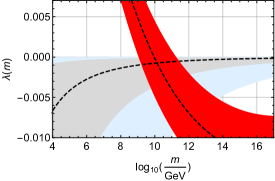
Figure 1: Matching of the Higgs quartic coupling at the scale $m$ in the SM (red band) with the prediction of Eq. (32), considering a Yukawa coupling spread of $\delta=\pm 0.6$ (light blue band), $\delta=\pm 0.3$ (light gray band), and $\delta=0$ (dashed black line). The intersection corresponds to the allowed range for $m$. See text for details.

In Fig. 1 we show the SM running of $\lambda(m)$ in red (the band takes into account the uncertainty in the initial conditions) and the RHS of Eq. (32) for $\delta=\pm 0.6$ (light blue band), $\delta=\pm 0.3$ (light gray band), and $\delta=0$ (dashed black line). We notice that the matching is possible only for negative values of $\lambda(m)$, which selects $10^{9}\,\text{GeV}\lesssim m\lesssim 10^{14}\,\text{GeV}$. By recalling $f^{2}/2m^{2}\simeq 0.23$, we conclude that

$$7\times 10^{8}\,\text{GeV}\lesssim f\lesssim 7\times 10^{13}\,\text{GeV}.$$ (33)

Since the flavon expectation value, $f$, is related to the axion decay constant by $f_{a}=f/N$,

$$N=\sum_{i}2H_{\Psi_{q_{L}}^{i}}-H_{\Psi_{u_{R}}^{i}}-H_{\Psi_{d_{R}}^{i}}\approx 50,$$ (34)

the previous bound yields

$$10^{7}\,\text{GeV}\lesssim\,f_{a}\,\lesssim 10^{12}\,\text{GeV}.$$ (35)

It is useful to confront this region with constraints following from the flavour-violating couplings of the axiflavon. In fact, limits from searches for the decay $K^{+}\to\pi^{+}a$ lead to $f_{a}\gtrsim 7.5\times 10^{10}$  GeV at $90\%$ C.L. Calibbi et al. (2017), leaving a relatively thin stripe of

$$f_{a}\approx(10^{11}-10^{12})\,\text{GeV}.$$ (36)

Interestingly, this range will almost entirely be tested by the NA62 experiment, which just started operation Anelli et al. (2005); Fantechi (2014).

III.1 Including right-handed neutrinos

We now discuss the impact of including right-handed (RH) neutrinos. Let us consider one family first. The left-handed doublet $l_{\mathrm{L}}$ and the RH neutrino $N_{\mathrm{R}}$ come as $\mathrm{SO}(5)$ spurions (see Eq. (6)):

$$\Psi_{\mathrm{L}}=\Delta^{T}_{\mathrm{L}}l_{\mathrm{L}},\quad\Psi_{N}=\Delta_{u}^{T}N_{\mathrm{R}}.$$ (37)

One possibility is to assign flavour charge to $\Psi_{N}$ such that the following term is allowed:

$$\begin{split}-\mathcal{L}_{N}=&\frac{1}{\sqrt{2}}y_{N}\bar{\Psi}_{N}\Sigma^{\prime}{\cal C}\bar{\Psi}_{N}^{T}+\text{h.c.}\\ =&-\frac{1}{2}y_{N}f\,\cos(h/f)\bar{N}_{\mathrm{R}}{\cal C}\bar{N}_{\mathrm{R}}^{T}e^{\imath a/f}+\text{h.c.},\end{split}$$ (38)

which yields a Majorana mass

$$m_{N_{\mathrm{R}}}^{2}(h)=y_{N}^{2}f^{2}\,\cos^{2}(h/f).$$ (39)

The Dirac mass term, $m_{\mathrm{D}}$, is obtained by integrating out the FN chain:

$$m_{\mathrm{D}}\sim m_{t}\epsilon^{\frac{|\delta_{\nu}|-1}{2}},$$ (40)

where $\delta_{\nu}=H_{l_{L}}-H_{N_{\mathrm{R}}}$. The light neutrino mass, $m_{\nu}$, is then given by

$$m_{\nu}\sim m_{t}\epsilon^{|\delta_{\nu}|-1}\frac{m_{t}}{m_{N_{\mathrm{R}}}},$$ (41)

which shows a double suppresion, originating from the type-I seesaw Minkowski (1977); Gell-Mann et al. (1979); T. Yanagida (1979); Mohapatra and Senjanovic (1980) and from the FN mechanism. The impact of Eq. (38) to the Higgs potential is

$$\begin{split}\Delta V_{\text{AFH}}^{(1)}=&-\frac{2}{64\pi^{2}}m^{4}_{N_{R}}(h)\left(\log\frac{m^{2}_{N_{R}}(h)}{m^{2}}-\frac{3}{2}\right)\\ =&-\frac{1}{32\pi^{2}}y_{N}^{4}f^{4}\cos^{4}(h/f)\left[\log\left(y_{N}^{2}\frac{f^{2}}{m^{2}}\right)\right.\\ &\left.\hskip 42.67912pt+\log\left(1-\sin(h/f)^{2}\right)-\frac{3}{2}\right]\\ \simeq&-\frac{1}{16\pi^{2}}y_{N}^{4}\left(1+\log\frac{1}{\tilde{\epsilon}}\right)f^{4}\text{sin}^{2}(h/f)\\ &+\frac{1}{32\pi^{2}}y_{N}^{4}\log\frac{1}{\tilde{\epsilon}}f^{4}\text{sin}^{4}(h/f)\,,\end{split}$$ (42)

where we have defined $(y_{N}f/m)^{2}=\tilde{\epsilon}$. At the leading order in $f^{2}/2m^{2}$, the matching conditions now read

$$\mu^{2}(m)=\frac{f^{2}}{16\pi^{2}}\left[2y_{N}^{4}\left(1+\log\frac{1}{\tilde{\epsilon}}\right)-N_{c}\gamma_{0}\right],$$ (43)

and

$$\lambda(m)=\frac{1}{8\pi^{2}}\log\frac{1}{\tilde{\epsilon}}\,y_{N}^{4}.$$ (44)

Assuming three almost degenerate RH neutrinos, with a typical coupling $y_{N}$ parametrized as $y_{N}=(1+\delta)y_{t}$, Eq. (44) becomes

$$\lambda(m)=\frac{3}{8\pi^{2}}\log\left(\frac{1}{2y_{t}^{2}(m)(1+\delta)^{2}\epsilon}\right)(1+\delta)^{4}y_{t}^{4}(m).$$ (45)

Figure 2: Matching of the Higgs quartic coupling at the scale $m$ in the SM (red band) with the prediction of Eq.(45), considering a yukawa spread of $\delta=\pm 0.6$ (light blue band), $\delta=\pm 0.3$ (light gray band), and $\delta=0$ (dashed black line). The intersection corresponds to the allowed range for $m$. See text for details.

In Fig. 2 we show the SM running of $\lambda(m)$ in red and the RHS of Eq. (45) for $\delta=\pm 0.6$ (light blue band), $\delta=\pm 0.3$ (light gray band) and $\delta=0$ (dashed black line). The matching is now possible for smaller values of $m$ with respect to the case without RH neutrinos, because the RHS of Eq. (45) is positive. The allowed region for $f$ is:

$$3\times 10^{5}\,\text{GeV}\lesssim f\lesssim 10^{11}\text{GeV}.$$ (46)

Furthermore, since $m_{N_{\mathrm{R}}}\simeq y_{N}\,f$ with $y_{N}\approx 1$, Eq. (46) also sets the range of the RH neutrino masses. Eventually, we find:

$$6\,\text{TeV}\lesssim f_{a}\lesssim 2\times 10^{6}\,\text{TeV}\,.$$ (47)

Such values of $f_{a}$ are excluded for the usual QCD axion, however, by disentangling the axion mass and decay constant, low-$f_{a}$ models can become viable. Recent concrete examples have been presented in Refs Gherghetta et al. (2016); Gaillard et al. (2018). Supernova cooling and flavour constraints can then be avoided by pushing the axion mass to the GeV or TeV scale. As a consequence, the axion cannot be a dark matter candidate, since it is no longer stable on cosmological scales, but still solves the strong CP problem. In addition, the RH neutrinos can provide a link to matter-antimatter asymmetry via leptogenesis Alanne et al. (2017).

III.2 Bounds from inflation

The inflationary Hubble scale, $H_{I}$, is constrained by the CMB measurement of the tensor-to-scalar ratio as Ade et al. (2014)

$$\frac{H_{I}}{2\pi}\leq 1.4\times 10^{13}\,\text{GeV}.$$ (48)

Since the reheating temperature, $T_{\text{RH}}$, is bounded by $H_{I}$, one obtains $T_{\text{RH}}\lesssim 10^{16}\,\text{GeV}$  Fairbairn et al. (2015). The expression for $T_{\text{RH}}$ is model dependent and is given by Chung et al. (1999)

$$T_{\text{RH}}=\left(\frac{45}{4\pi^{3}g_{*}}\right)^{1/4}\left(\Gamma_{\phi}M_{\text{Pl}}\right)^{1/2},$$ (49)

where $\Gamma_{\phi}$ is the width of the inflaton field and $g_{*}$ is the number of relativistic degrees of freedom.

Our aim is to extract a cosmological constraint on the Peccei–Quinn scale when the flavon field itself plays the role of the inflaton, $\phi=\sigma$ Antusch et al. (2008); Fairbairn et al. (2015); Ema et al. (2017). Note that in order to have a successful inflation, one needs, for instance, to introduce a non-minimal coupling to gravity.

To estimate the constraint, we compute $\Gamma_{\sigma}$ in our model. The flavon field couples at the tree-level to the other scalars in the $\Sigma$-multiplet and to RH neutrinos if the interaction in Eq. (38) is included. The potential in Eq. (2) is stable for $\lambda_{1}>\lambda_{2}>0$. We focus here in the limit where $\lambda_{1}\gg\lambda_{2}$, such that all the scalar decay channels for $\sigma$ are open, and the width is thus maximised. The width into scalars is then given by

$$\Gamma_{\sigma}^{(s)}=N_{s}\frac{1}{8\pi^{2}}\frac{\lambda_{1}}{2}m_{\sigma}=N_{s}\frac{1}{8\pi^{2}}(\lambda_{1})^{3/2}f\,,$$ (50)

where $N_{s}=9$ is the number of scalar decay channels, corresponding to two scalar doublets and the axion. Including RH neutrinos, which contribute

$$\begin{split}\Gamma_{\sigma}^{(N_{\mathrm{R}})}=\frac{3}{32\pi^{2}}y_{N}^{2}m_{\sigma}=\frac{3}{16\pi^{2}}(\lambda_{1})^{1/2}y_{N}^{2}f\,,\end{split}$$ (51)

we arrive at an upper bound on $f$ of

$$\begin{split}f_{a}\cdot N=f\leq&\ \frac{8\pi^{2}}{\left(\lambda_{1})^{1/2}(N_{s}\lambda_{1}+\frac{1}{2}\sum_{i}g_{i}^{2}\right)}\left(\frac{4\pi^{3}g_{*}}{45}\right)^{1/2}\\ &\times\left(\frac{10^{16}\,\text{GeV}}{M_{\text{Pl}}}\right)\,10^{16}\,\text{GeV}.\end{split}$$ (52)

This leads to a relevant bound only in the high-scale model without RH neutrinos, since the one with RH neutrinos easily avoids this constraint due to the relatively low scale $f$. Taking $g_{*}=\mathcal{O}(100)$ and $y_{N}=0$, we find

$$f_{a}\lesssim 3\,(\lambda_{1})^{-3/2}\,10^{13}\,\text{GeV}\,.$$ (53)

In the extreme case of $\lambda_{1}=4\pi$ (for which $\Gamma_{\sigma}$ almost equals $m_{\sigma}$), $f_{a}\lesssim 10^{12}\,\text{GeV}$, which is the same upper bound as in Eq. (35).

IV Conclusions

We presented a model framework where the flavour puzzle, the strong CP problem, and the origin of the observed DM abundance are solved by a single scalar multiplet which also contains the Higgs boson. The latter emerges as a pNGB of an enhanced global symmetry, thereby connecting the EWSB with the origin of the SM-fermion mass hierarchies. To achieve this, we provided a renormalizable UV realization of the FN mechanism.

We showed that successfully reproducing the SM-like Higgs potential at low energies fixes the axion decay constant to $f_{a}\approx(10^{11}-10^{12})\,\text{GeV}$ for the minimal setup, where the lower bound is driven from limits on flavour-changing axion couplings. This lies just in a region where axions are a very attractive DM candidate, and which is a prime target of future searches, in particular at NA62 and ADMX Asztalos et al. (2010); Du et al. (2018).

We also demonstrated that by including RH neutrinos, the symmetry-breaking scale could be lowered bringing the axion decay constant down to TeV range and commented on the possibility of the flavon component to be identified with the inflaton.

Appendix A The validity of the FN mass degeneracy assumption

Let us discuss the implication of relaxing the degeneracy among the FN messengers. We paramatrize the departure from the degenerate case by introducing $\delta_{j}$ parameters:

$$\begin{split}m^{2}_{\xi_{j}}&=m^{2}(1+\delta_{j})+f_{j}(h)=m^{2}+(m^{2}\delta_{j}+f_{j}(h))\\ &\equiv m^{2}+\tilde{f}_{j}(h).\end{split}$$ (54)

The previous analysis now applies with $f_{j}(h)$ replaced by $\tilde{f}_{j}(h)$. The condition under which the non-degeneracy effects can be neglected then reads:

$$m^{2}\delta_{j}\ll f\times m\Rightarrow\delta_{j}\ll f/m=\sqrt{2\epsilon}\sim 0.68$$ (55)

We conclude that the non-degeneracy can be neglected as long as $\delta_{j}\ll 0.7$.

Appendix B Subleading contributions to the Higgs potential

Similarly to the top eigenstate, the contribution of the gauge bosons will appear on both sides of Eq. (20) and thus do not alter the one-loop matching condition; the same reasoning applies to the other SM eigenstates. However, an additional contribution is expected when the FN messengers mixing with the light fermions are included.

For concreteness, let us consider the up-type quarks. The Yukawa interactions before diagonalization read

$$\mathcal{L}_{u}=-y_{ij}\epsilon^{n_{ij}}\bar{q}_{L}^{\,i}\tilde{H}u_{R}^{\,j}+{\rm h.c.}\,,$$ (56)

where $y_{ij}=\mathcal{O}(1)$, where the hierarchies

$$n_{ij}=\left(\begin{array}[]{ccc}8&4&3\\ 7&3&2\\ 5&1&0\end{array}\right)$$ (57)

lead to a viable spectrum Ema et al. (2017). Thus, by recalling the relation between $\mathrm{U}(1)_{\mathrm{H}}$ charge differences and the suppresion factor Eq. (14), we shall require

$$\frac{|\delta_{ij}|-1}{2}=n_{ij}.$$ (58)

Looking at the second-third family mixing, we see that it can be reproduced by assigning the $H$ charges

$$H_{{t_{\mathrm{L}}}}=1,\ H_{{t_{\mathrm{R}}}}=2,\ H_{{c_{\mathrm{L}}}}=-3,\ H_{{c_{\mathrm{R}}}}=4.$$ (59)

The charm sector can then be written in a similar way as in Eq. (15), according to the charge assignments, Eq. (59). The contribution to the Higgs potential is found to be $\mathcal{O}(f^{2}/2m^{2})$ for the $\text{sin}^{2}(h/f)$ and $\mathcal{O}(f^{4}/4m^{4})$ for the $\text{sin}^{4}(h/f)$ term, which is subleading compared to the top sector. The same reasoning applies to all light SM fermions.

References

- Froggatt and Nielsen (1979) C. D. Froggatt and H. B. Nielsen, Nucl. Phys. B147, 277 (1979).
- Calibbi et al. (2017) L. Calibbi, F. Goertz, D. Redigolo, R. Ziegler, and J. Zupan, Phys. Rev. D95, 095009 (2017), arXiv:1612.08040 [hep-ph] .
- Ema et al. (2017) Y. Ema, K. Hamaguchi, T. Moroi, and K. Nakayama, JHEP 01, 096 (2017), arXiv:1612.05492 [hep-ph] .
- Peccei and Quinn (1977) R. D. Peccei and H. R. Quinn, Phys. Rev. Lett. 38, 1440 (1977), [,328(1977)].
- Wilczek (1978) F. Wilczek, Phys. Rev. Lett. 40, 279 (1978).
- Weinberg (1978) S. Weinberg, Phys. Rev. Lett. 40, 223 (1978).
- Kim (1979) J. E. Kim, Phys. Rev. Lett. 43, 103 (1979).
- Shifman et al. (1980) M. A. Shifman, A. I. Vainshtein, and V. I. Zakharov, Nucl. Phys. B166, 493 (1980).
- Dine et al. (1981) M. Dine, W. Fischler, and M. Srednicki, Phys. Lett. 104B, 199 (1981).
- Zhitnitsky (1980) A. R. Zhitnitsky, Sov. J. Nucl. Phys. 31, 260 (1980), [Yad. Fiz.31,497(1980)].
- Preskill et al. (1983) J. Preskill, M. B. Wise, and F. Wilczek, Phys. Lett. B120, 127 (1983), .
- Abbott and Sikivie (1983) L. F. Abbott and P. Sikivie, Phys. Lett. B120, 133 (1983), .
- Dine and Fischler (1983) M. Dine and W. Fischler, Phys. Lett. B120, 137 (1983), .
- Redi and Strumia (2012) M. Redi and A. Strumia, JHEP 11, 103 (2012), arXiv:1208.6013 [hep-ph] .
- Alanne et al. (2015) T. Alanne, H. Gertov, F. Sannino, and K. Tuominen, Phys. Rev. D91, 095021 (2015), arXiv:1411.6132 [hep-ph] .
- Alanne et al. (2016) T. Alanne, A. Meroni, F. Sannino, and K. Tuominen, Phys. Rev. D93, 091701 (2016), arXiv:1511.01910 [hep-ph] .
- Kaplan (1991) D. B. Kaplan, Nucl. Phys. B365, 259 (1991).
- Agashe et al. (2005) K. Agashe, R. Contino, and A. Pomarol, Nucl. Phys. B719, 165 (2005), arXiv:hep-ph/0412089 [hep-ph] .
- Anelli et al. (2005) G. Anelli et al., CERN-SPSC-2005-013, CERN-SPSC-P-326 (2005).
- Fantechi (2014) R. Fantechi (NA62), in 12th Conference on Flavor Physics and CP Violation (FPCP 2014) Marseille, France, May 26-30, 2014 (2014), arXiv:1407.8213 [physics.ins-det] .
- Minkowski (1977) P. Minkowski, Phys. Lett. 67B, 421 (1977).
- Gell-Mann et al. (1979) M. Gell-Mann, P. Ramond, and R. Slansky, Supergravity, edited by F. Nieuwenhuizen and D. Friedman (North Holland, Amsterdam, 1979) p. 315.
- T. Yanagida (1979) T. Yanagida, “Proc. of the Workshop on Unified Theories and the Baryon Number of the Universe,” KEK, Japan (1979).
- Mohapatra and Senjanovic (1980) R. N. Mohapatra and G. Senjanovic, Phys. Rev. Lett. 44, 912 (1980).
- Gherghetta et al. (2016) T. Gherghetta, N. Nagata, and M. Shifman, Phys. Rev. D93, 115010 (2016), arXiv:1604.01127 [hep-ph] .
- Gaillard et al. (2018) M. K. Gaillard, M. B. Gavela, R. Houtz, P. Quilez, and R. Del Rey, (2018), arXiv:1805.06465 [hep-ph] .
- Alanne et al. (2017) T. Alanne, A. Meroni, and K. Tuominen, Phys. Rev. D96, 095015 (2017), arXiv:1706.10128 [hep-ph] .
- Ade et al. (2014) P. A. R. Ade et al. (Planck), Astron. Astrophys. 571, A22 (2014), arXiv:1303.5082 [astro-ph.CO] .
- Fairbairn et al. (2015) M. Fairbairn, R. Hogan, and D. J. E. Marsh, Phys. Rev. D91, 023509 (2015), arXiv:1410.1752 [hep-ph] .
- Chung et al. (1999) D. J. H. Chung, E. W. Kolb, and A. Riotto, Phys. Rev. D60, 063504 (1999), arXiv:hep-ph/9809453 [hep-ph] .
- Antusch et al. (2008) S. Antusch, S. F. King, M. Malinsky, L. Velasco-Sevilla, and I. Zavala, Phys. Lett. B666, 176 (2008), arXiv:0805.0325 [hep-ph] .
- Asztalos et al. (2010) S. J. Asztalos et al. (ADMX), Phys. Rev. Lett. 104, 041301 (2010), arXiv:0910.5914 [astro-ph.CO] .
- Du et al. (2018) N. Du et al. (ADMX), Phys. Rev. Lett. 120, 151301 (2018), arXiv:1804.05750 [hep-ex] .