SUPERIORIZATION OF PRECONDITIONED CONJUGATE GRADIENT ALGORITHMS FOR TOMOGRAPHIC IMAGE RECONSTRUCTION

Abstract.

Properties of Superiorized Preconditioned Conjugate Gradient (SupPCG) algorithms in image reconstruction from projections are examined. Least squares (LS) is usually chosen for measuring data-inconsistency in these inverse problems. Preconditioned Conjugate Gradient algorithms are fast methods for finding an LS solution. However, for ill-posed problems, such as image reconstruction, an LS solution may not provide good image quality. This can be taken care of by superiorization. A superiorized algorithm leads to images with the value of a secondary criterion (a merit function such as the total variation) improved as compared to images with similar data-inconsistency obtained by the algorithm without superiorization. Numerical experimentation shows that SupPCG can lead to high-quality reconstructions within a remarkably short time. A theoretical analysis is also provided.

1. Introduction

Superiorization [7, 5, 1, 3, 4] is an algorithmic framework that consists in perturbing iterative methods. It can be applied to feasibility problems (problems of finding a point belonging to a given set) or to optimization problems (problems of finding the best point among a set of candidates, according to some criterion). Its aim is to improve the iterates, according to a secondary criterion (which is some sort of merit function), produced by an iterative method for solving the original problem without the secondary criterion.

Many problems in science or engineering can be mathematically modeled as feasibility [2] or optimization [6] problems. In this paper we use tomographic imaging as our example application of the superiorized algorithms that we introduce, but the basic idea is useful in numerous other contexts.

We investigate a superiorized Preconditioned Conjugate Gradient (PCG) method, applying it to tomographic imaging and comparing it to other approaches to this application. In Section 2 we connect tomographic image reconstruction to optimization, as in [6]. Section 3 reviews superiorization, the Conjugate Gradient (CG) and the PCG algorithms. Superiorization of these algorithms results in the algorithms Superiorized Conjugate Gradient (SupCG) and Superiorized Preconditioned Conjugate Gradient (SupPCG), and superiorization of one of the Algebraic Reconstruction Techniques (ART) [6, Chapter 11] leads to SupART. Section 4 reports on numerical experiments comparing the performance in image reconstruction of these algorithms, as well as a version of ART that uses blob basis functions [6, Section 6.5]. Section 5 presents a theoretical analysis of the SupPCG algorithm. Finally, Section 6 provides the concluding remarks.

2. Optimization in tomographic reconstruction

Assume that the image $x\in\mathbb{R}^{n}$ generates the data $b\in\mathbb{R}^{m}$ through

$$Rx=b_{exact}+e,$$

where $R\in\mathbb{R}^{m\times n}$ is the projection (also called Radon) matrix, $b=b_{exact}+e$, and $e\in\mathbb{R}^{m}$ is the unknown error vector introduced into the measurements. Therefore, we need to solve $Rx\approx b\text{,}$ where the meaning of the approximation must be well defined mathematically. There are several ways of doing this, in the present paper we follow the least squares approach:

(2.1) $$x\in\operatorname*{arg\,min}_{y\in\mathbb{R}^{n}}\|Ry-b\|^{2}\text{.}$$

Because the least squares approach is well accepted and extremely general, it is not surprising that several techniques have been developed for its solution. The minimizers in (2.1) are given by the solutions of the normal equations

(2.2) $$R^{T}Rx=R^{T}b\text{,}$$

which is a linear system of equations. Due to the huge size and sparsity of the projection matrix (as can be the case in image reconstruction), iterative methods that successively approximate a solution may be the most practical.

Among the best-known iterative techniques for the general problem of least squares, one can point at CG and at PCG, to be applied to the system (2.2); see [11]. For tomographic image reconstruction, algebraic reconstruction techniques (ART) [6, Chapter 11] are widely applied.

To put this into a general context, let $f$ be a function defined over images such that $f(x)$ is some measure of the inconsistency of $x$ with the given data. The primary aim of a proposed reconstruction method should be to produce an $x$ for which the value of $f$ is relatively small, therefore $f$ is referred to as the primary criterion. Here we concentrate on the squared error, $f(x)=\|Rx-b\|^{2}$, as the primary criterion. We also discuss a primary criterion based on a Bayesian approach to image reconstruction [8], namely

(2.3) $$r^{2}\left\|Rx-b\right\|^{2}+\left\|x-\mu_{X}\right\|^{2},$$

where the number $r$ is the so-called signal-to-noise ratio and $\mu_{X}$ is a uniformly gray image with the gray value being the average value of the image as can be accurately estimated based on all the measured data [6, Section 6.4]. Both these need to be specified for a particular reconstruction task.

3. Superiorization of PCG and ART

3.1. Superiorization

As stated in [1]:

The superiorization methodology is used for improving the efficacy of iterative algorithms whose convergence is resilient to certain kinds of perturbations. Such perturbations are designed to “force” the perturbed algorithm to produce more useful results for the intended application than the ones that are produced by the original iterative algorithm. The perturbed algorithm is called the “superiorized version” of the original unperturbed algorithm. If the original algorithm is computationally efficient and useful in terms of the application at hand and if the perturbations are simple and not expensive to calculate, then the advantage of this method is that, for essentially the computational cost of the original algorithm, we are able to get something more desirable by steering its iterates according to the designed perturbations.

Several iterative algorithms use an updating of the current approximation to the problem at hand that is of the form

$$\left(x_{k+1},u_{k+1}^{1},\dots,u_{k+1}^{\nu}\right)=\mathit{\mathrm{U}}\left(x_{k},u_{k}^{1},\dots,u_{k}^{\nu}\right),$$

where the $u_{k}^{i}$ for $1\leq i\leq\nu$ are some auxiliary vectors and $x_{k}$ is the image at iteration $k$. A superiorized version of such a method can have the form

(3.1) $$\left(x_{k+1},u_{k+1}^{1},\dots,u_{k+1}^{\nu}\right)=\mathit{\mathrm{U}}\left(x_{k+\nicefrac{{1}}{{2}}},u_{k}^{1},\dots,u{}_{k}^{\nu}\right)\text{,}$$

where $x_{k+\nicefrac{{1}}{{2}}}=x_{k}+s_{k}$, with $\{s_{k}\}$ referred to as a superiorization sequence. For our experiments in Section 4 we used the method from [7], as specified in Algorithm 1, for generating the superiorization sequence. The actual values produced by that specification depend on the chosen secondary criterion and the procedure to compute “nonascending vectors” for this criterion; here we report on results for total variation ($TV$) as the secondary criterion (see [7, 3, 4]).

Total variation is defined for a vector $y\in\mathbb{R}^{n}$ that represents a discrete image $[y]$ with $l$ rows and $c$ columns of pixels with $lc=n$. The value $[y]_{i,j}$ of the pixel in the $i$th row and $j$th column of this image is defined to be the $(c(i-1)+j)$th component of vector $y$. The definition of total variation is

$$TV(y):=\sum_{i=1}^{l-1}\sum_{j=1}^{c-1}\sqrt{\left([y]_{(i,j)}-[y]_{(i+1,j)}\right)^{2}+\left([y]_{(i,j)}-[y]_{(i,j+1)}\right)^{2}}.$$

Algorithm 1 uses nonascending vectors. Following [7], given a point $y\in\mathbb{R}^{n}$, we say that $t\in\mathbb{R}^{n}$ is a nonascending vector for $TV$ at $y$ if $\|t\|\leq 1$ and there is $\Delta>0$ such that

$$\delta\in[0,\Delta]\Rightarrow TV(y+\delta t)\leq TV(y).$$

We denote the set of nonascending vectors for $TV$ at $y$ as $\tilde{\partial}TV(y)$. Note that $\tilde{\partial}TV(y)$ is never empty because the zero vector is in $\tilde{\partial}TV(y)$. In order to get the $t\in\tilde{\partial}TV(y)$ that we actually use, first define $\overline{t}\in\mathbb{R}^{n}$ componentwise. For any component of $\overline{t}$, its value is the negative of the partial derivative of $TV$ at $y$ with respect to that component, if this partial derivative is well defined, and is $0$ otherwise. We finally define the nonascending vector $t\in\tilde{\partial}TV(y)$ that we use as

$$t=\begin{cases}\frac{\overline{t}}{\|\overline{t}\|},&\text{if }\left\|\overline{t}\right\|\neq 0,\\ \mathrm{the\>zero\>vector},&\text{otherwise.}\end{cases}$$

That the $t$ specified this way is indeed a nonascending vector for $TV$ at $y$ is an immediate consequence of [7, Theorem 2].

The specification of Algorithm 1 involves further parameters: $K\in\mathbb{N}$ (the number of nonascending steps), $a\in(0,1)$ (the step-length diminishing factor for each nonascending trial) and $\gamma\in(0,\infty)$ (the starting step-length); for complete specification, these parameters need to be selected by the user. Next we provide details of the purpose and operation of Algorithm 1.

Algorithm 1 $\mathrm{S}_{TV}(x,\ell,a,\gamma,K)$

1:  $y\leftarrow x$

2:  for $i=1,2,\dots,K$

3:     $t\in\tilde{\partial}TV(y)$

4:     repeat

5:        $\tilde{\gamma}\leftarrow\gamma a^{\ell}$

6:        $\tilde{y}\leftarrow y+\tilde{\gamma}t$

7:        $\ell\leftarrow\ell+1$

8:     until $TV(\tilde{y})\leq TV(y)$

9:     $y\leftarrow\tilde{y}$

10:  return $(y-x,\ell)$

Algorithm 1 specifies the $s_{k}$ to be used to define $x_{k+\nicefrac{{1}}{{2}}}=x_{k}+s_{k}$, which is then further used to provide us with the next image $x_{k+1}$ of the superiorized iterative algorithm, see (3.1). As the iterations proceed, changes are made not only to the image vector but also to an integer variable $\ell$ (see Step 7 of Algorithm 1), these changes are needed to make the superiorized algorithm behave as desired (see [7, 12] and Section 5 below). In the superiorized algorithm, $\ell$ is initialized to be $0$ (that is why $\gamma$ is referred to as the starting step-length). In each step (3.1) of the superiorized iterative algorithm, Algorithm 1 is called with the current values of the image vector $x_{k}$, the integer $\ell$ and the user-specified parameters $a$, $\gamma$ and $K$ (these do not change during an execution of the superiorized algorithm). Algorithm 1 returns $s_{k}\left(=y-x_{k}\right)$ and the new value of $\ell$, to be used in the next iterative step of the algorithm. During the execution of the superiorized algorithm, the step lengths $\tilde{\gamma}$ form a summable sequence as needed in the theoretical results on the behavior of superiorized algorithms (see, for example, [7, Theorem 1]).

Superiorization has, by design, an influence over algorithmic convergence, but ideally it maintains the required properties of the limit point. The influence of the superiorization should be that the sequence of iterates $\{x_{k}\}$ (or $\{x_{k+\nicefrac{{1}}{{2}}}\}$) for the superiorized method has reduced secondary criterion (in our case, $TV$) when compared to the equivalent sequence produced by the unsuperiorized method. For our method this is true because the superiorization step, although only guaranteed not to increase the value of the undifferentiable $TV$ criterion, is frequently capable of actually reducing the value of the $TV$. That is, one usually finds that $TV(x_{k+\nicefrac{{1}}{{2}}})<TV(x_{k})$.

We provide a theoretical discussion of the convergence of the SupPCG algorithm in Section 5. A convergence proof of the SupCG algorithm appears in [12] and that result is extended naturally to the superiorized version of the PCG algorithm, which is a method that we now proceed to discuss.

3.2. Preconditioned Conjugate Gradient

The CG algorithm is designed to solve a linear system of equations $Ax=y$, where $A$ is symmetric positive semi-definite. If $A=R^{T}R$ and $y=R^{T}b$, then CG can solve (2.1) via (2.2). The CG method may converge slowly depending on the distribution of the eigenvalues of the system matrix $A$. The idea of PCG is to replace the system $Ax=y$ by a preconditioned system $MAx=My$, where $M$ is a symmetric positive-definite matrix, so that the two systems have the same solutions but $MA$ has better spectral properties for the application of the CG algorithm. We return to this topic later in Section 5.

Algorithm 2 $\mathrm{U}_{\text{PCG}}$$(x,p,h)$

1:  $g\leftarrow Ax-y$

2:  $z\leftarrow Mg$

3:  $\beta\leftarrow z^{T}h/p^{T}h$

4:  $p\leftarrow-z+\beta p$

5:  $h\leftarrow Ap$

6:  $\alpha\leftarrow-g^{T}p/p^{T}h$

7:  $x\leftarrow x+\alpha p$

8:  return $(x,p,h)$

Given $\mathrm{U}_{\text{PCG}}$ defined by Algorithm 2, the update for PCG algorithm is

$$\left(x_{k+1},p_{k},h_{k}\right)=\mathrm{U_{\text{PCG}}}\left(x_{k},p_{k-1},h_{k-1}\right)\text{,}$$

where $x_{0}\in\mathbb{R}^{n}$ is an arbitrary vector, but $x_{1}$, $p_{0}$ and $h_{0}$ must follow precise rules, as described for SupPCG in the next subsection. The preconditioning matrix $M$ that we use here is of the form $F^{-1}DF$, where $F$ is the Discrete Fourier Transform (DFT) and $D$ is a diagonal matrix that represents a generalized Hamming window [6] (using parameters $\mu$ and $\rho$) combined with a ramp filter for frequency $\omega$ with $-\pi\leq\omega\leq\pi$:

(3.2) $$h(\omega)=(|\omega|+\mu)\cdot(\rho+(1-\rho)\cos\omega).$$

3.3. Superiorized Preconditioned Conjugate Gradient

In this subsection we describe, as Algorithm 3, the SupPCG method, which is the main subject of the present paper. In its specification, we use the notations $f(x)=\|Rx-b\|^{2}$, $A=R^{T}R$ and $y=R^{T}b$; see (2.1) and (2.2). The inputs of Algorithm 3 are the initial image $x_{0}$, the $a$, $\gamma$ and $K$ that have the same roles as in Algorithm 1 and a user-specified $\varepsilon>0$ that determines the termination of Algorithm 3 (see Step 10). The algorithm returns the number of iterations $k$ at the time of its termination and an output image $x_{k-\nicefrac{{1}}{{2}}}$.

Algorithm 3 SupPCG$\left(x_{0},a,\gamma,K,\varepsilon\right)$

1:  $x_{\nicefrac{{1}}{{2}}}\leftarrow x_{0}$

2:  $g_{0}\leftarrow Ax_{0}-y$

3:  $z_{0}\leftarrow Mg_{0}$

4:  $p_{0}\leftarrow-z_{0}$

5:  $h_{0}\leftarrow Ap_{0}$

6:  $\alpha\leftarrow-g_{0}^{T}p_{0}/p_{0}^{T}h_{0}$

7:  $x_{1}\leftarrow x_{0}+\alpha p_{0}$

8:  $k\leftarrow 1$

9:  $\ell_{1}\leftarrow 0$

10:  while $f\left(x_{k-\nicefrac{{1}}{{2}}}\right)>\varepsilon$

11:     $(s_{k},\ell_{k+1})\leftarrow\mathrm{S}_{TV}\left(x_{k},\ell_{k},a,\gamma,K\right)$

12:     $x_{k+\nicefrac{{1}}{{2}}}\leftarrow x_{k}+s_{k}$

13:     $(x_{k+1},p_{k},h_{k})\leftarrow\mathrm{U}_{\text{PCG}}\left(x_{k+\nicefrac{{1}}{{2}}},p_{k-1},h_{k-1}\right)$

14:     $k\leftarrow k+1$

15:  $\textbf{return }\left(k,x_{k-\nicefrac{{1}}{{2}}}\right)$

For the termination of Algorithm 3 to be guaranteed by the results we present in Section 5, we will need appropriate bounds on the elements of the superiorization sequence $\left\{s_{k}\right\}$; we now provide such bounds.

Theorem 1.

Upon the execution of Step 11 in Algorithm 3, we have that $\|s_{k}\|\leq K\gamma a^{(k-1)K}$.

Proof.

To verify this assertion, we first note that the vectors $t\in\tilde{\partial}TV(y)$ in Algorithm 1 satisfy $\|t\|\leq 1$, by the definition of nonascending vectors as given above. Next we prove inductively that $\ell_{k}\geq(k-1)K$. This inequality holds for $k=1$ as an equality. Now assume, for the induction, that it holds for iteration $k$. The value of $\ell_{k+1}$ is determined by Step 11 of Algorithm 3, which consists in a call $\mathrm{S}_{TV}\left(x_{k},\ell_{k},a,\gamma,K\right)$ to Algorithm 1. In each of the $K$ loops of Algorithm 1 (see its Step 2), $\ell$ is increased at least once (in Step 7). This and the induction hypothesis implies that for the $\ell_{k+1}$ returned by $\mathrm{S}_{TV}\left(x_{k},\ell_{k},a,\gamma,K\right)$, we have $\ell_{k+1}\geq\ell_{k}+K\geq\left(k-1\right)K+K=kK=\left((k+1\right)-1)K;$ this completes the inductive proof.

We introduce some extra notations. Consider the call $\mathrm{S}_{TV}(x_{k},\ell_{k},a,\gamma,K)$ to Algorithm 1 in Algorithm 3. In the execution of that call, there is an inner loop (indexed by $i$) consisting of Steps 3-9 of Algorithm 1. We now use $t_{k,i}$ to denote the value of $t$ obtained by Step 3 in that inner loop and $\ell_{k,i}$ as $\ell-1$ at the time when the condition $TV(\tilde{y})\leq TV(y)$ in Step 8 of the inner loop is satisfied. Looking at $\mathrm{S}_{TV}\left(x_{k},\ell_{k},a,\gamma,K\right)$, we see that for the $s_{k}$ returned by Step 11 of Algorithm 3 we have that $s_{k}=\gamma\sum_{i=1}^{K}a^{\ell_{k,i}}t_{k,i}$. Since $\left\|t_{k,i}\right\|\leq 1$, $\ell_{k,i}\geq\ell_{k}\geq(k-1)K$ and $a\in(0,1)$, we conclude that $\left\|s_{k}\right\|\leq\gamma\sum_{i=1}^{K}\left\|a^{\ell_{k,i}}t_{k,i}\right\|\leq\gamma\sum_{i=1}^{K}a^{\ell_{k,i}}\left\|t_{k,i}\right\|\leq\gamma\sum_{i=1}^{K}a^{\ell_{k}}\leq K\gamma a^{(k-1)K}$. ∎

3.4. Superiorized Algebraic Reconstruction Technique

The Algebraic Reconstruction Techniques consist of sequentially projecting the current image toward the hyperplanes defined by the equations of a linear system and we consider a full cycle through the equations to be a single iteration. Several variants are possible, we use the version originally proposed in [8] with pixel basis functions (we refer to this as ART) and also with blob basis functions [10], see alternatively [6, Section 6.5] (we refer to this as BlobART). We also report on superiorization using the $TV$ secondary criterion for the pixel basis, we refer to the so superiorized ART as SupART.

To be more specific, the ART method proposed in [8] (see alternatively [6, Section 11.3]) aims at finding the minimizer of the primary criterion given in (2.3). Therefore the signal-to-noise ratio $r$ is a parameter that needs to be specified for both ART and for BlobART. There is an additional parameter $\lambda$ for these algorithms, it is the so-called relaxation parameter that determines the size of the step in projecting the current image toward the next hyperplane. Mathematical convergence theory allows the relaxations to vary with iterations [6, 8], and this may be useful in practice, but here we choose a single $\lambda$ for a reconstruction run.

4. Numerical experimentation

4.1. Tomographic data acquisition simulation

We used data obtained from simulation of a phantom that includes features such as seen in medical images [6, Fig. 4.6(a)]. The phantom has low-contrast features of interest inside a high attenuation skull-like structure. If shown in its full grayscale range, the inner features are nearly invisible, therefore the phantom and reconstructions are displayed using a gray scale in which linear attenuation values smaller than $0.204\;\text{cm}^{-1}$ are displayed as black and values higher than $0.21675\>\text{cm}^{-1}$ appear as white. Phantom and tomographic data were obtained using SNARK14. (SNARK14 is the most recent version of a series of software packages for the reconstruction of 2D images from 1D projections. From the point of view of the current paper, its main advantage over the previous version SNARK09 [9] is the new ability to superiorize automatically any iterative algorithm.) The phantom can be seen at the bottom-right of Fig. 4.1. It consists of an array of $243\times 243$ pixels, each of which corresponds to an area of $0.0752\times 0.0752\;\text{cm}^{2}$. Data were collected for $360$ equally spaced angles in $[0,\pi)$ and each of these angles was sampled for $345$ parallel rays spaced at $0.0752\;\text{cm}$ between them. Random photon emission at the x-ray source and scattering of the x-ray photons was simulated.

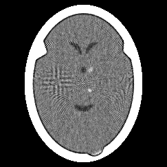
(a) PCG, iteration 2

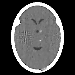
(b) SupPCG, iteration 3

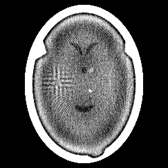
(c) CG, iteration 12

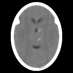
(d) SupCG, iteration 35

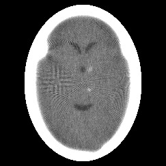
(e) ART, iteration 15

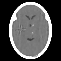
(f) SupART, iteration 12

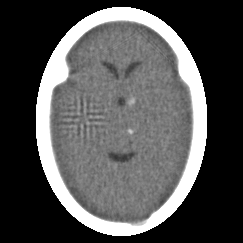
(g) BlobART, iteration 14

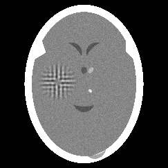
(h) Phantom

Figure 4.1. Phantom and best images obtained by each algorithm. The best images are those that for which (i) the parameters have been selected according to the method described in Subsection 4.2 and specified in Table 1, and (ii) the value of the selective error (the $SE$ of (4.1)) is the smallest among all the ones plotted in Fig. 4.2.

4.2. Algorithmic parameter selection

The compared algorithms, with the exception of CG, have parameters to be tuned. To select these parameters, we evaluated the quality of the reconstructed image $x$ using the figure of merit called selective error ($SE$) and then chose, for each algorithm separately, the parameters that provided the best reconstructed image within the first $15$ iterations. $SE$ is defined by

(4.1) $$SE(x)=C\sqrt{\sum_{(i,j)\in S}\left([x]_{i,j}-[x^{\dagger}]_{i,j}\right)^{2}}\text{,}$$

where $C$ is a constant dependent on the phantom $x^{\dagger}$ and $S$ is the set of pixels contained in a centered ellipse with a $5$ cm horizontal and a $7$ cm vertical semi-axis. This ellipse is just inside the “skull” in the phantom.

All the superiorized methods share three parameters ($K$, $a$ and $\gamma$, see Algorithm 1 and 3 ) that were drawn from the following sets: $K\in\{10,20,40\}$, $a\in\{1-10^{-5},1-10^{-4},\dots,1-10^{-1}\}$, $\gamma\in\{10^{-2},5\cdot 10^{-2}\}$. PCG and SupPCG have two preconditioning parameters: $\mu\in\{10^{-5},10^{-4},10^{-3}\}$ and $\rho\in\{0.4,0.6,0.8\}$; see (3.2). ART, BlobART and SupART use the signal-to-noise ratio $r\in\{5,10\}$, which corresponds to the parameter with the same symbol in [8, eq. (7)] (where the version of ART we use here is described) and a relaxation parameter $\lambda\in\{10^{-2},5\cdot 10^{-2},10^{-1},5\cdot 10^{-1},1\}$; see also [6, Section 11.3]. The combination of parameters, within the sets specified above, that provided the best results are listed in Table 1.

Method	Optimal Parameters
SupCG	$(K,a,\gamma)=\left(40,1-10^{-5},5\cdot 10^{-2}\right)$
PCG	$(\mu,\rho)=\left(10^{-3},0.6\right)$
SupPCG	$(K,a,\gamma,\mu,\rho)=\left(40,1-10^{-5},10^{-2},10^{-5},0.8\right)$
ART and BlobART	$(r,\lambda)=\left(5,10^{-2}\right)$
SupART	$(K,a,\gamma,r,\lambda)=\left(10,1-10^{-5},10^{-2},5,5\cdot 10^{-2}\right)$

Table 1. Optimal parameters for compared algorithms.

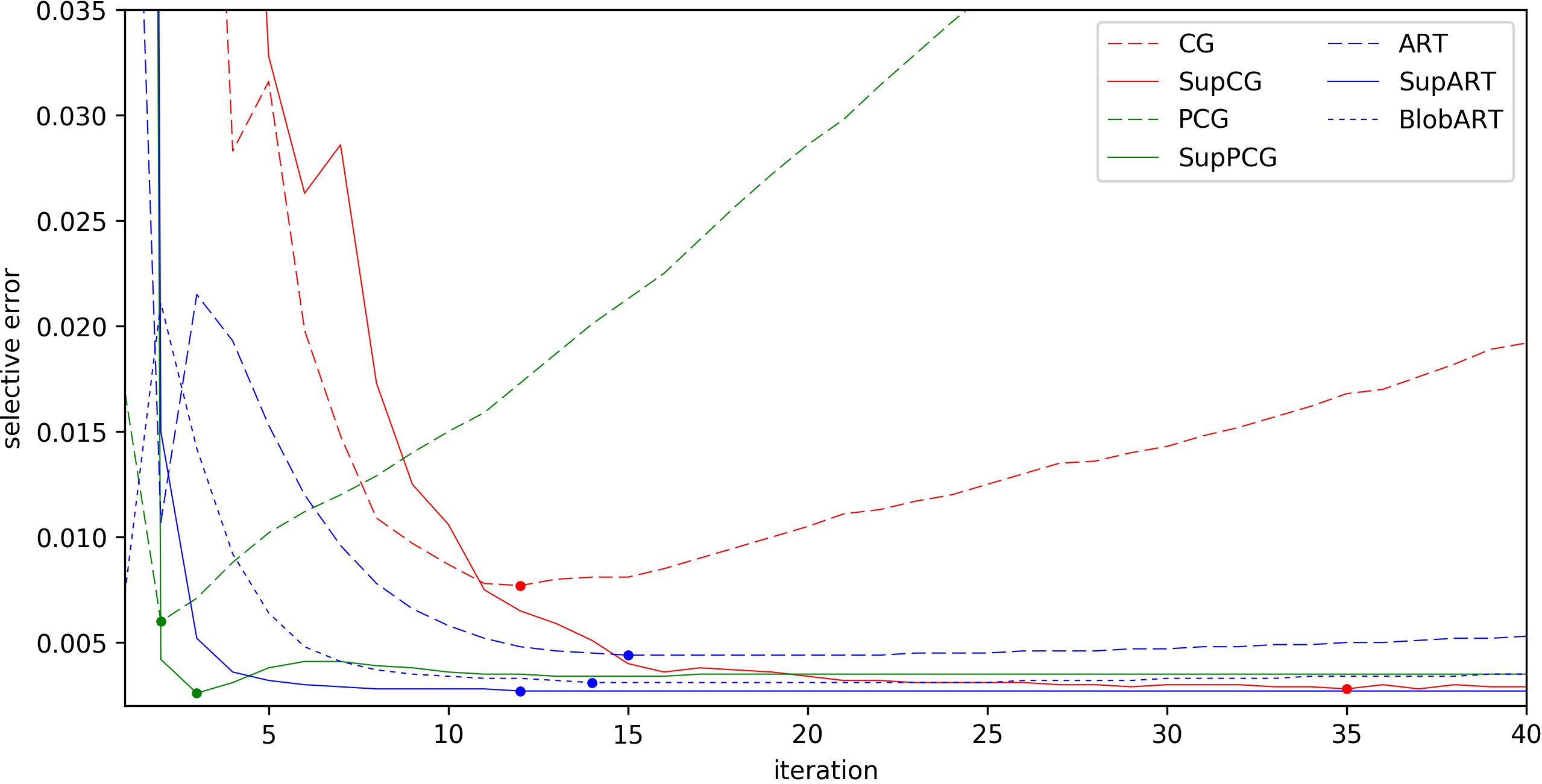
Figure 4.2. Iteration-wise comparison of $SE$ evolution among algorithms. Location of the smallest $SE$ value on each curve is indicated.

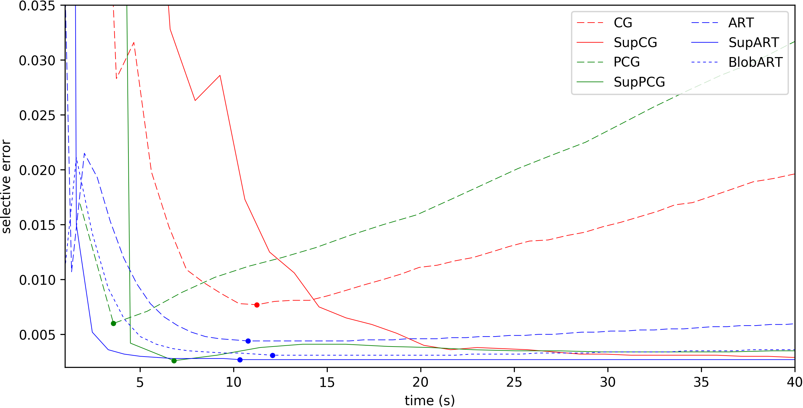
Figure 4.3. Time-wise comparison of $SE$ evolution among algorithms. Location of the smallest $SE$ value on each curve is indicated.

4.3. Numerical results

In Fig. 4.2 we present the evolution of the $SE$ of (4.1) as iterations proceed, while Figure 4.3 exhibits a time-wise comparison among the methods. The computer used to run the methods had an Intel i7 7700HQ processor running at up to 3.4GHZ with 32GB of RAM available for the computations. We notice that a superiorized method obtains better values for the $SE$ figure of merit than the corresponding unsuperiorized version for almost every iteration. This does not come as a surprise, for two reasons. First, the superiorized version is supposed to incorporate better prior knowledge about the sought-after image to be reconstructed through the secondary criterion. Second, in the experiments we present, the algorithmic parameter settings were tailored to obtain an improved value of the figure of merit $SE$.

5. Theoretical Analysis

In the present section we prove that the SupPCG method (Algorithm 3) terminates under a suitable hypothesis on the superiorization sequence $\left\{s_{k}\right\}$ that is defined by calling $\mathrm{S}_{TV}(x_{k},a,\gamma,K)$. Our proof is based on facts established in [12], which contains a proof that SupCG terminates. The needed relation between the SupPCG and the SupCG is established via the so-called Transformed PCG algorithm (TPCG) and its superiorized version (SupTPCG). Next we discuss these algorithms.

Since the preconditioning matrix $M$ is symmetric positive-definite, there exists an invertible matrix $N$ such that $M=N^{T}N$ and, for such a matrix, the eigenvalues of $MA$ are the same as the eigenvalues of $NAN^{T}$ (if $v$ is an eigenvector of $MA$, then $N^{-T}v$ is an eigenvector of $NAN^{T}$ with the same associated eigenvalue). Applying one step of the CG algorithm (which is exactly Algorithm 2 with $M$ the identity matrix) to the linear system $NAN^{T}\hat{x}=Ny$ provides one step of TPCG, as given in Algorithm 4. This step is also called from SupTPCG, see Step 13 of Algorithm 5.

There is a strict equivalence between Algorithm 3 and Algorithm 5. To see this consider Table 2. We claim, and this can be verified by following step-by-step SupPCG$\left(x_{0},a,\gamma,K,\varepsilon\right)$ and SupTPCG$\left(N^{-T}x_{0},a,\gamma,K,\varepsilon\right)$, that the behavior of the two algorithms are identical via the stated equivalences. In particular, since $f\left(x_{k-\nicefrac{{1}}{{2}}}\right)=f\left(N^{T}\hat{x}_{k-\nicefrac{{1}}{{2}}}\right)$, the two algorithms terminate for the same value of $k$ and the two images returned by the respective algorithms can be obtained from each other using $x_{k+\nicefrac{{1}}{{2}}}=N^{T}\hat{x}_{k+\nicefrac{{1}}{{2}}}$.

Algorithm 4 $\mathrm{U}_{\text{TPCG}}$$\left(\hat{x},\hat{p},\hat{h}\right)$

1:  $\hat{g}\leftarrow NAN^{T}\hat{x}-Ny$

2:  $\hat{z}\leftarrow\hat{g}$

3:  $\beta\leftarrow\hat{z}{}^{T}\hat{h}/\hat{p}^{T}\hat{h}$

4:  $\hat{p}\leftarrow-\hat{z}+\beta\hat{p}$

5:  $\hat{h}\leftarrow NAN^{T}\hat{p}$

6:  $\alpha\leftarrow-\hat{g}^{T}\hat{p}/\hat{p}^{T}\hat{h}$

7:  $\hat{x}\leftarrow\hat{x}+\alpha\hat{p}$

8:  return $\left(\hat{x},\hat{p},\hat{h}\right)$

Algorithm 5 SupTPCG$\left(\hat{x}_{0},a,\gamma,K,\varepsilon\right)$

1:  $\hat{x}_{\nicefrac{{1}}{{2}}}\leftarrow\hat{x}_{0}$

2:  $\hat{g}_{0}\leftarrow NAN^{T}\hat{x}_{0}-Ny$

3:  $\hat{z}_{0}\leftarrow\hat{g}_{0}$

4:  $\hat{p}_{0}\leftarrow-\hat{z}_{0}$

5:  $\hat{h}_{0}\leftarrow NAN^{T}\hat{p}_{0}$

6:  $\alpha\leftarrow-\hat{g}_{0}^{T}\hat{p}_{0}/\hat{p}_{0}^{T}\hat{h}_{0}$

7:  $\hat{x}_{1}\leftarrow\hat{x}_{0}+\alpha\hat{p}_{0}$

8:  $k\leftarrow 1$

9:  $\ell_{1}\leftarrow 0$

10:  while $f\left(N^{T}\hat{x}_{k-\nicefrac{{1}}{{2}}}\right)>\varepsilon$

11:     $\left(s_{k},\ell_{k+1}\right)\leftarrow\mathrm{S}_{TV}\left(N^{T}\hat{x}_{k},\ell_{k},a,\gamma,K\right)$

12:  $\mbox{\quad}\hat{x}_{k+\nicefrac{{1}}{{2}}}\leftarrow\hat{x}_{k}+N^{-T}s_{k}$

13:     $\left(\hat{x}_{k+1},\hat{p}_{k},\hat{h}_{k}\right)\leftarrow\mathrm{U}_{\text{TPCG}}\left(\hat{x}_{k+\nicefrac{{1}}{{2}}},\hat{p}_{k-1},\hat{h}_{k-1}\right)$

14:     $k\leftarrow k+1$

15:  $\textbf{return }\left(k,\hat{x}_{k-\nicefrac{{1}}{{2}}}\right)$

Algorithm 3	Algorithm 5
$x_{i}=N^{T}\hat{x}_{i}$	$\hat{x}_{i}$
$g_{0}$	$\hat{g}_{0}=Ng_{0}$
$z_{0}=N^{T}\hat{z}_{0}$	$\hat{z}_{0}$
$p_{k}=N^{T}\hat{p}_{k}$	$\hat{p}_{k}$
$h_{k}$	$\hat{h}_{k}=Nh_{k}$

Table 2. Equivalences of the variables in Algorithm 3 and Algorithm 5. The $i$ in the table can be $k$, $k-\nicefrac{{1}}{{2}}$, or $k+\nicefrac{{1}}{{2}}$ for an integer $k$.

Next we show the equivalence of Algorithm 5 and Algorithm 7 of [12] under some assumptions. To make the current paper self-contained, we reproduce here (as Algorithm 7) Algorithm 7 of [12]. We keep the boldface notation of [12] in order to avoid confusion with the symbols used in the algorithms introduced in the present paper. Consistently with the notation of that previous paper, the function $f^{\prime}$ in Algorithm 7 is defined by

(5.1) $$f^{\prime}(\mathbf{x}) =\frac{1}{2}\|\mathbf{A}\mathbf{x}-\mathbf{y}\|^{2},$$

where $\mathbf{\mathit{\mathbf{A}}}=RN^{T}$ and $\mathbf{y}=b$.

As already defined in Subsection 3.3, $A=R^{T}R$ and $y=R^{T}b$. By setting $\mathbf{\mathit{\mathbf{A}}}$ and $\mathbf{\mathbf{y}}$ in Algorithm 8 of [12] (restated here as Algorithm 6) to be as we have just defined them, we see that Algorithm 4 is equivalent to Algorithm 8 of [12] in the sense that if we have in the input of the two algorithms the equivalences $\mathbf{x}=\hat{x}$, $\mathbf{p}=\hat{p}$, and $\mathbf{h}=\hat{h}$, then $\mathbf{g}=\hat{g}$ (to see this, notice that in Algorithm 4 we have $Ny=NR^{T}b=\mathbf{A}^{T}\mathbf{y}$, and $NAN^{T}=NR^{T}RN^{T}=\mathbf{A}^{T}\mathbf{A}$), the $\beta$ in the two algorithms are equal (since $\hat{z}=\hat{g}$) and, therefore, we also have that the output values satisfy $\mathbf{p}=\hat{p}$, $\mathbf{h}=\hat{h}$ (because $NAN^{T}=\mathbf{A}^{T}\mathbf{A}$) and $\mathbf{x}=\hat{x}$ (since, as is easily verified, the value of $\alpha$ is the same for the two algorithms). Thus, for identical inputs, Algorithms 4 and 6 will return identical outputs.

Algorithm 6 $\mathrm{U}_{\text{CG}}$$(\mathbf{x},\mathbf{p},\mathbf{h})$

1:  $\mathbf{g}\leftarrow\mathbf{A}^{T}(\mathbf{A\mathbf{x}}-\mathbf{y})$

2:  $\beta\leftarrow\mathbf{g}{}^{T}\mathbf{h}/\mathbf{p}^{T}\mathbf{h}$

3:  $\mathbf{p}\leftarrow-\mathbf{g}+\beta\mathbf{p}$

4:  $\mathbf{h}\leftarrow\mathbf{A}^{T}\mathbf{A}\mathbf{p}$

5:  $\alpha\leftarrow-\mathbf{g}{}^{T}\mathbf{p}/\mathbf{p}^{T}\mathbf{h}$

6:  $\mathbf{x}\leftarrow\mathbf{x}+\alpha\mathbf{p}$

7:  return $(\mathbf{x},\mathbf{p},\mathbf{h})$

Algorithm 7 SupCG$\left(\mathbf{x}_{0},a,\gamma,K,\varepsilon^{\prime}\right)$

1:  $\mathbf{x}_{\nicefrac{{1}}{{2}}}\leftarrow\mathbf{x}_{0}$

2:  $\mathbf{g}_{0}\leftarrow\mathbf{A}^{T}(\mathbf{A\mathbf{x}}_{0}-\mathbf{y})$

3:  $\mathbf{p}_{0}\leftarrow-\mathbf{g}_{0}$

4:  $\mathbf{h}_{0}\leftarrow\mathbf{A}^{T}\mathbf{A}\mathbf{p}_{0}$

5:  $\alpha\leftarrow-\mathbf{g}{}_{0}^{T}\mathbf{p}_{0}/\mathbf{p}_{0}^{T}\mathbf{h}_{0}$

6:  $\mathbf{x}_{1}\leftarrow\mathbf{x}_{0}+\alpha\mathbf{p}_{0}$

7:  $k\leftarrow 1$

8:  while $f^{\prime}(\mathbf{x}_{k-\nicefrac{{1}}{{2}}})>\varepsilon^{\prime}$

9:  $\mbox{\quad}\mathbf{x}_{k+\nicefrac{{1}}{{2}}}\leftarrow\text{{perturbed}}\left(\mathbf{x}_{k}\right)$

10:     $\left(\mathbf{x}_{k+1},\mathbf{p}_{k},\mathbf{h}_{k}\right)\leftarrow\mathrm{U}_{\text{PCG}}\left(\mathbf{x}_{k+\nicefrac{{1}}{{2}}},\mathbf{p}_{k-1},\mathbf{h}_{k-1}\right)$

11:     $k\leftarrow k+1$

12:  $\textbf{return }\left(k,\mathbf{x}_{k-\nicefrac{{1}}{{2}}}\right)$

To show the equivalence of Algorithm 5 and Algorithm 7, we associate $\mathbf{\mathit{\mathbf{x}}}_{k}$, $\mathbf{\mathit{\mathbf{x}}}_{k+\nicefrac{{1}}{{2}}}$, $\mathbf{\mathbf{g}}_{k}$, $\mathbf{\mathbf{h}}_{k}$, $\mathbf{p}_{k}$ in Algorithm 7 with $\hat{x}_{k}$, $\hat{x}_{k+\nicefrac{{1}}{{2}}}$, $\hat{g}_{k}$, $\hat{h}_{k}$, $\hat{p}_{k}$ in Algorithm 5 by $\mathbf{\mathit{\mathbf{x}}}_{k}=\hat{x}_{k}$, $\mathbf{x}_{k+\nicefrac{{1}}{{2}}}=\hat{x}_{k+\nicefrac{{1}}{{2}}}$, $\mathbf{g}_{k}=\hat{g}_{k}$, $\mathbf{\mathbf{h}}_{k}=\hat{h}_{k}$, $\mathbf{\mathbf{p}}_{k}=\hat{p}_{k}$. We now compare the step-by-step executions of SupTPCG$\left(\hat{x}_{0},a,\gamma,K,\varepsilon\right)$ and SupCG$\left(\mathbf{x}_{0},a,\gamma,K,\varepsilon^{\prime}\right)$, with $\mathbf{\mathit{\mathbf{x}}}_{0}=\hat{x}_{0}$ and $\varepsilon^{\prime}=\frac{\varepsilon}{2}$. Clearly, after Step 1 in the two algorithms $\mathbf{\mathit{\mathbf{x}}}_{\nicefrac{{1}}{{2}}}=\hat{x}_{\nicefrac{{1}}{{2}}}$. That $\mathbf{g}_{0}=\hat{g}_{0}$ follows from the facts that $Ny=\mathbf{A}^{T}\mathbf{y}$, and $NAN^{T}=\mathbf{A}^{T}\mathbf{A}$. Continuing in this fashion it is trivial to check that just before entering the $\mathbf{while}$ statement for the first time in the two algorithms the values of the associated vectors match as stated above.

We now consider the condition that appears in the $\mathbf{while}$ statement in the algorithms. We claim that if just before entering the $\mathbf{while}$ in the two algorithms the values of the associated vectors match as stated above, then the condition is either satisfied in both algorithms or is not satisfied in both algorithm. Indeed, due to the definition of $f$ as the squared error and (5.1),

$$f\left(N^{T}\hat{x}_{k-\nicefrac{{1}}{{2}}}\right)=\left\|RN^{T}\hat{x}_{k-\nicefrac{{1}}{{2}}}-b\right\|^{2}=\left\|\mathbf{A}\mathbf{x}_{k-\nicefrac{{1}}{{2}}}-\mathbf{y}\right\|^{2}=2f^{\prime}\left(\mathbf{x}_{k-\nicefrac{{1}}{{2}}}\right).$$

Since $\varepsilon^{\prime}=\frac{\varepsilon}{2}$, our claim on the satisfaction of the conditions is valid.

We specify the perturbation operator in Step 9 of Algorithm 7 by

$$\mathrm{perturbed}\left(\mathbf{x}_{k}\right)=\mathbf{x}_{k}+N^{-T}s_{k},$$

where $s_{k}$ is the same as given by Algorithm 5. Using the above associations and facts, we see that the behavior of Algorithm 5 is equivalent to that of Algorithm 7, and, therefore, to that of Algorithm 7 of [12].

Theorem A.1 of [12] says that SupCG$\left(\mathbf{x}_{0},a,\gamma,K,\varepsilon^{\prime}\right)$ terminates provided that $\varepsilon^{\prime}>\varepsilon_{0}^{\prime}$, where

$$\varepsilon_{0}^{\prime}=\min_{\mathbf{x}}\frac{1}{2}\|\mathbf{A}\mathbf{x}-\mathbf{y}\|^{2}.$$

Recalling the definitions of $\mathbf{A}$ and $\mathbf{y}$ after (5.1) and the fact that $N$ is invertible, we get that $\varepsilon^{\prime}_{0}=\frac{1}{2}\varepsilon_{0,}$ for

$$\varepsilon_{0}=\min_{\hat{x}}\left\|RN^{T}\hat{x}-b\right\|^{2}=\min_{x}\left\|Rx-b\right\|^{2}.$$

This together with the comparison of the the step-by-step executions of SupTPCG$\left(\hat{x}_{0},a,\gamma,K,\varepsilon\right)$ and SupCG$\left(\mathbf{x}_{0},a,\gamma,K,\varepsilon^{\prime}\right)$, with $\mathbf{\mathit{\mathbf{x}}}_{0}=\hat{x}_{0}$ and $\varepsilon^{\prime}=\frac{\varepsilon}{2}$, gives us our promised termination result for SupPCG:

Theorem 2.

Given any positive number $\varepsilon$ such that $\varepsilon>\varepsilon_{0}$, with

(5.2) $$\varepsilon_{0}=\min_{x}\left\|Rx-b\right\|^{2},$$

Algorithm 3 terminates within a finite number of iterations.

6. Concluding remarks

We have discussed the superiorized version of the Preconditioned Conjugate Gradient method (SupPCG) for tomographic image reconstruction. Experimental work has been presented indicating that, when compared to several other methods, SupPCG produces images of good quality within a short time. Furthermore, we have proved that the algorithm produces, in a finite number of steps, an image whose data-inconsistency is no worse than what is specified by the user, provided that such an image exists.

References

- [1] Y. Censor, G. T. Herman, and M. Jiang. Superiorization: theory and applications. Inverse Problems, 33, 040301, 2017.
- [2] P. L. Combettes. The convex feasibility problem in image recovery. Advances in Imaging and Electron Physics, 95:155–270, 1996.
- [3] E. Garduño and G. T. Herman. Superiorization of the ML-EM algorithm. IEEE Transactions on Nuclear Science, 61:162–172, 2014.
- [4] E. Garduño and G. T. Herman. Computerized tomography with total variation and with shearlets. Inverse Problems, 33, 044011, 2017.
- [5] E. S. Helou, M. V. W. Zibetti, and E. X. Miqueles. Superiorization of incremental optimization algorithms for statistical tomographic image reconstruction. Inverse Problems, 33, 044010, 2017.
- [6] G. T. Herman. Fundamentals of Computerized Tomography: Image Reconstruction from Projections. Springer, London, UK, 2nd. edition, 2009.
- [7] G. T. Herman, E. Garduño, R. Davidi, and Y. Censor. Superiorization: An optimization heuristic for medical physics. Medical Physics, 39:5532–5546, 2012.
- [8] G. T. Herman, H. Hurwitz, A. Lent, and H.-P. Lung. On the Bayesian approach to image reconstruction. Information and Control, 42:60–71, 1979.
- [9] J. Klukowska, R. Davidi, and G. T. Herman. SNARK09 - A software package for the reconstruction of 2D images from 1D projections. Computer Methods and Programs in Biomedicine, 110:424–440, 2013.
- [10] R. Marabini, G. T. Herman, and J. M. Carazo. 3D reconstruction in electron microscopy using ART with smooth spherically symmetric volume elements (blobs). Ultramicroscopy, 72:53–65, 1998.
- [11] C. R. Vogel. Computational Methods for Inverse Problems. SIAM, Philadelphia, PA, 2002.
- [12] M. V. W. Zibetti, C. Lin, and G. T. Herman. Total variation superiorized conjugate gradient method for image reconstruction. Inverse Problems, 34, 034001, 2018.