Lattice Boltzmann study of the one-dimensional boost-invariant expansion with anisotropic initial conditions

Abstract

A numerical algorithm for the implementation of anisotropic distributions in the frame of the relativistic Boltzmann equation is presented. The implementation relies on the expansion of the Romatschke-Strickland distribution with respect to orthogonal polynomials, which is evolved using the lattice Boltzmann algorithm. The validation of our proposed scheme is performed in the context of the one-dimensional boost invariant expansion (Bjorken flow) at various values of the ratio $\eta/s$ of the shear viscosity to the entropy density. This study is limited to the case of massless particles obeying Maxwell-Jüttner statistics.

1 INTRODUCTION

Following the seminal work of Israel and Stewart [1], relativistic viscous fluid dynamics has been continuously developed for a wide range of applications, including stellar collapse [2], accretion problems [3], cosmology [4] and the quark-gluon plasma (QGP) [5] (see [6] for a recent review).

The formation of the QGP was highlighted in the mid-rapidity range of ultra-high energy heavy ion collisions during the experiments performed at the Relativistic Heavy Ion Collider (RHIC) (for a historical account, please see Ref. [7]). The experimental evidence validated the boost-invariant longitudinal expansion model proposed by Bjorken [8], which was initially solved in the perfect fluid approximation.

Even though the experimental evidence confirmed that the QGP exhibited an extremely low shear viscosity ($\eta$) to entropy density ($s$) ratio, the time scale of its lifespan and the pressure anisotropy induced by the longitudinal expansion prevent the QGP from settling into complete thermodynamic equilibrium, as required for a perfect fluid. Indeed, through the adS/CFT conjecture, it was determined that $\eta/s=\hbar/4\pi k_{B}$ for relativistic conformal field theories at finite temperature and zero chemical potential [9]. In the conditions prevalent during the lifetime of the QGP, viscosities of this order of magnitude can induce significant deviations from the perfect fluid limit [10].

The construction of a relativistic viscous hydrodynamics theory has proven to be a formidable challenge, since the correspondent of the Navier-Stokes equations represents a first order formulation which is non-causal [11]. The validation of second [12] and even third [13] order hydrodynamics equations relied on the semi-analytic solution of the relativistic Boltzmann equation for the one-dimensional boost-invariant longitudinal expansion [14]. However, all hydrodynamic formulations seem to break down when $\eta/s$ becomes larger than some critical value [15]. Thus, it is clear that in order to perform realistic relativistic fluid dynamics simulations of QGP phenomena, it is necessary to develop an efficient kinetic solver. This is the argument that motivates the present work.

The lattice Boltzmann method was recently employed to obtain solutions of the relativistic Boltzmann equation, including for the one-dimensional boost-invariant longitudinal expansion [16, 17]. The implementation in Ref. [17] was validated against the semi-analytic solution of the Bjorken flow presented in Ref. [14] for massless particles obeying Maxwell-Jüttner statistics at vanishing chemical potential, but only for the case of isotropic initial conditions. Since it is expected that the strong longitudinal expansion induces a non-negligible pressure anisotropy, it is necessary that the scheme developed in Ref. [17] be extended to the case of anisotropic initial conditions, which we implement by using the Romatschke-Strickland form [18]. This is the main result of this paper. The resulting scheme is validated by comparison with first and second order hydrodynamics results at small $\eta/s$, analytic expressions in the free-streaming regime and the semi-analytic procedure derived in Ref. [14] everywhere else.

2 RELATIVISTIC BOLTZMANN EQUATION FOR THE BJORKEN FLOW

The Bjorken flow is characterized by the assumption that the QGP properties in the mid-rapidity region (the central plateau) are invariant under Lorentz boosts along the longitudinal direction [8]. This assumption fixes the macroscopic four-velocity at $u^{t}=t/\tau$ and $u^{z}=z/\tau$ while neglecting the transverse dynamics (i.e., $u^{x}=u^{y}=0$), where $\tau=\sqrt{t^{2}-z^{2}}$ is the proper time. The analysis of the flow properties is simplified by introducing the Milne coordinates $(\tau,x,y,\eta_{M})$, where $\eta_{M}=\tanh^{-1}(z/t)$ is the space-time rapidity, with respect to which the Minkowski line element becomes $ds^{2}=-d\tau^{2}+dx^{2}+dy^{2}+\tau^{2}d\eta_{M}^{2}$. It is convenient to introduce the following tetrad vector frame $e_{\hat{\alpha}}$ ($e_{\hat{\tau}}=\partial_{\tau}$, $e_{\hat{x}}=\partial_{x}$, $e_{\hat{y}}=\partial_{y}$ $e_{{\hat{\eta}}_{M}}=\tau^{-1}\partial_{\eta_{M}}$) and its associated one-form coframe $\omega^{\hat{\alpha}}$ such that $p^{\hat{\alpha}}=\omega^{\hat{\alpha}}_{\mu}p^{\mu}$ [17].

As a first approximation, the QGP can be effectively described as a parton gas dominated by (massless) gluons obeying Maxwell-Jüttner statistics at vanishing chemical potential [14, 17]. The mass shell condition $\eta_{{\hat{\alpha}}{\hat{\beta}}}p^{\hat{\alpha}}p^{\hat{\beta}}=0$ implies that $p^{{\hat{\tau}}}=\sqrt{(p^{\hat{x}})^{2}+(p^{\hat{y}})^{2}+(p^{{\hat{\eta}}_{M}})^{2}}\equiv p$. The non-dimensionalised Maxwell-Jüttner equilibrium distribution $f^{\rm{(eq)}}$ at vanishing chemical potential can be written as:

$$f^{\rm{(eq)}}=\frac{\widetilde{p}_{\rm ref}^{3}}{\widetilde{n}^{\rm(eq)}_{0}}\widetilde{f}^{\rm(eq)}=\frac{1}{8\pi}e^{-p/T},$$ (1)

where $\widetilde{p}_{\rm ref}=\widetilde{k}_{B}\widetilde{T}_{0}/\widetilde{c}$ is the reference momentum, $\widetilde{n}_{0}^{\rm(eq)}=8\pi g_{s}(\widetilde{k}_{B}\widetilde{T}_{0}/2\pi\widetilde{\hbar}\widetilde{c})^{3}$ is the initial equilibrium parton number density at vanishing chemical potential and initial temperature $\widetilde{T}_{0}$, $g_{s}=16$ represents the gluon number of degrees of freedom, while the temperature $T=P^{1/4}$ is given in terms of the isotropic pressure $P$ of the parton gas.

The evolution of the parton distribution function $f\equiv f(\tau;p,\xi)$ which depends on the momentum magnitude $p$ and $\xi=p^{{\hat{\eta}}_{M}}/p^{\hat{\tau}}$ is given by the relativistic Boltzmann equation written with respect to tetrad fields [19] as [17]:

$$\partial_{\tau}f+\frac{1}{\tau}f-\frac{\xi^{2}}{\tau p^{2}}\partial_{p}(fp^{3})-\frac{1}{\tau}\partial_{\xi}[\xi(1-\xi^{2})f]=-\frac{1}{\tau_{\rm{A-W}}}[f-f^{\rm{(eq)}}],$$ (2)

where the gas is assumed to be homogeneous with respect to the space-time rapidity $\eta_{M}$ and transverse coordinates $x$ and $y$. The right hand side of the above equation represents the Anderson-Witting approximation of the Boltzmann collision integral and the relaxation time $\tau_{\rm A-W}$ is given by [17]:

$$\tau_{\rm A-W}=\frac{\tau_{\rm A-W;0}}{P^{1/4}},\qquad\tau_{\rm A-W;0}=\frac{5\hbar(\overline{\eta/s})}{\widetilde{\tau_{0}}\widetilde{k}_{B}\widetilde{T}_{0}}\simeq 0.523426\times\frac{0.25\ {\rm fm}}{\widetilde{c}\widetilde{\tau}_{0}}\times\frac{600\ {\rm MeV}}{\widetilde{k}_{B}\widetilde{T}_{0}}\times 4\pi(\overline{\eta/s}).$$ (3)

The above implementation of $\tau_{\rm A-W}$ ensures that the shear viscosity to entropy density ratio $(\overline{\eta/s})$ is constant for sufficiently small values of $\tau_{\rm A-W}$ [14] (the overline denotes that the ratio is expressed in Planck units). The analysis in this paper is restricted to the case when $\widetilde{c}\widetilde{\tau}_{0}=0.25\ {\rm fm}$ and $\widetilde{k}_{B}\widetilde{T}_{0}=600\ {\rm MeV}$. The longitudinal and transverse pressures $\mathcal{P}_{L}$ and $\mathcal{P}_{T}$, the isotropic pressure $P$ and the pressure deviator $\Pi$ can be computed as moments of $f$:

$$\mathcal{P}_{L}=\int\frac{d^{3}p}{p^{\hat{\tau}}}f\,(p^{{\hat{\eta}}_{M}})^{2},\qquad\mathcal{P}_{T}=\int\frac{d^{3}p}{p^{\hat{\tau}}}f\,(p^{\hat{x}})^{2}=\int\frac{d^{3}p}{p^{\hat{\tau}}}f\,(p^{\hat{y}})^{2},\qquad P=\frac{1}{3}(\mathcal{P}_{L}+2\mathcal{P}_{T}),\qquad\Pi=\frac{2}{3}(\mathcal{P}_{L}-\mathcal{P}_{T}).$$ (4)

In order to allow for an anisotropy of the distribution function at the initial time $\tau=\tau_{0}=1$, $f$ can be initialized using the Romatschke-Strickland form [18], which has the following dimensionful expression:

$$\widetilde{f}_{\rm R-S}=\frac{g_{s}}{(2\pi\widetilde{\hbar})^{3}}\exp\left[-\frac{1}{\widetilde{\Lambda}_{0}}\sqrt{(\widetilde{p}\cdot\widetilde{u})^{2}+\xi_{0}\widetilde{c}^{2}(\widetilde{p}\cdot z)^{2}}\right],$$ (5)

where $\xi_{0}>-1$ is a measure of the initial pressure anisotropy along the direction of the unit vector $z$ and $\widetilde{\Lambda}_{0}$ is an energy scale fixed by specifying the initial temperature. In the case of the Bjorken flow, $u^{\hat{\alpha}}=(1,0,0,0)^{T}$ and $z^{\hat{\alpha}}=(0,0,0,1)$ is the space-time rapidity unit vector, such that Eq. (5) can be expressed in non-dimensional form as:

$$f_{\rm R-S}=\frac{1}{8\pi}\exp\left[-\frac{p}{\Lambda_{0}}\sqrt{1+\xi_{0}\xi^{2}}\right],\qquad\Lambda_{0}=\left[\frac{1}{2}\left(\frac{1}{\sqrt{\xi_{0}}}\arctan\sqrt{\xi_{0}}+\frac{1}{1+\xi_{0}}\right)\right]^{-1/4},$$ (6)

valid for any $\xi_{0}>0$. The initial longitudinal $\mathcal{P}_{L,0}$ and transverse $\mathcal{P}_{T,0}$ pressures are:

$$\mathcal{P}_{L,0}=\frac{3\Lambda_{0}^{4}}{2\xi_{0}}\left[\frac{1}{\sqrt{\xi_{0}}}\arctan\sqrt{\xi_{0}}-\frac{1}{1+\xi_{0}}\right],\qquad\mathcal{P}_{T,0}=\frac{3\Lambda_{0}^{4}}{4\xi_{0}}\left(1+\frac{\xi_{0}-1}{\sqrt{\xi_{0}}}\arctan\sqrt{\xi_{0}}\right),$$ (7)

while $P_{0}=1$. The initial pressure deviator $\Pi_{0}$ is:

$$\Pi_{0}=-\frac{\Lambda_{0}^{4}}{2\xi_{0}}\left[\frac{\xi_{0}+3}{\xi_{0}+1}+\frac{1}{\sqrt{\xi_{0}}}(\xi_{0}-3)\arctan\sqrt{\xi_{0}}\right]=-\left[1-\frac{3}{\xi_{0}}+\frac{6}{\xi_{0}+\sqrt{\xi_{0}}(\xi_{0}+1)\arctan\sqrt{\xi_{0}}}\right].$$ (8)

3 LATTICE BOLTZMANN ALGORITHM

In order to solve Eq. (2), we employ the lattice Boltzmann algorithm introduced in Ref. [17], which we extend in order to account for the anisotropic initial conditions given by Eq. (6). The momentum space is discretized following the prescriptions of Gauss quadratures with respect to the spherical coordinates $(p,\theta,\varphi)$. Since the flow is isotropic in the transverse plane, the $\varphi$ degree of freedom is integrated analytically. The magnitude $p$ of the momentum is discretised using the generalized Gauss-Laguerre quadrature of order $Q_{L}=2$ [$L_{Q_{L}}^{(2)}(p_{k})=0$, $1\leq k\leq Q_{L}$], while the Gauss-Legendre quadrature of order $Q_{\xi}$ is used to discretise $\xi=\cos\theta$ [$P_{Q_{\xi}}(\xi_{j})=0$, $1\leq j\leq Q_{\xi}$]. The above discretization allows $\mathcal{P}_{L}$ and $\mathcal{P}_{T}$ (4) to be computed using the following quadrature sums [17]:

$$\mathcal{P}_{T}=\frac{1}{2}\sum_{j=1}^{Q_{\xi}}\sum_{k=1}^{Q_{L}}f_{jk}p_{k}(1-\xi_{j}^{2}),\qquad\mathcal{P}_{L}=\sum_{j=1}^{Q_{\xi}}\sum_{k=1}^{Q_{L}}f_{jk}p_{k}\xi_{j}^{2},$$ (9)

where $f_{jk}=2\pi e^{p_{k}}w_{j}^{\xi}w_{k}^{L}f(p_{k},\xi_{j})$, while $w_{k}^{L}$ and $w_{j}^{\xi}$ are the Gauss-Laguerre and Gauss-Legendre quadrature weights.

In order to ensure conservation of energy-momentum, the equilibrium distribution $f^{\rm{(eq)}}$ appearing on the right hand side of Eq. (2) is replaced by a truncated series with respect to the Laguerre and Legendre polynomials. In the particular case of the Bjorken flow, $f^{\rm{(eq)}}$ does not depend on $\xi$, such that its expansion is simply:

$$f^{\rm{(eq)}}_{jk}=\frac{1}{4}n^{\rm(eq)}w_{j}w_{k}[1+(1-T)(3-p_{k})],\qquad n^{\rm(eq)}=P^{3/4},\qquad T=P^{1/4},$$ (10)

while $P=\frac{1}{3}(2\mathcal{P}_{T}+\mathcal{P}_{L})$ is obtained using the moments (9) of $f$. Starting from the expansion of $f$ with respect to the Laguerre and Legendre polynomials, the derivatives with respect to $p$ and $\xi$ appearing in Eq. (2) can be written as $\left[p^{-2}\partial_{p}(fp^{3})\right]_{jk}=\sum_{k^{\prime}=1}^{Q_{L}}\mathcal{K}^{L}_{k,k^{\prime}}f_{j,k^{\prime}}$ and $\left\{\partial_{\xi}[\xi(1-\xi^{2})f]\right\}_{jk}=\sum_{j^{\prime}=1}^{Q_{\xi}}\mathcal{K}^{P}_{j,j^{\prime}}f_{j^{\prime},k}$, where the kernels $\mathcal{K}^{L}_{k,k^{\prime}}$ $\mathcal{K}^{P}_{j,j^{\prime}}$ are given in Ref. [17]. The time stepping in Eq. (2) is performed using a third order Runge-Kutta algorithm [20] with $\delta\tau=10^{-3}$.

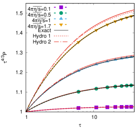
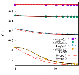
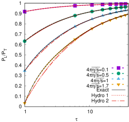
Figure 1: Comparison between LB results (lines and points), first-order (dotted lines) and second-order (dash-dotted lines) hydrodynamics and the semi-analytic exact solution reported in Ref. [14] [shown using solid lines only for $4\pi(\overline{\eta/s})>0.1$], for $P$ (left), $\Pi$ (center) and $\mathcal{P}_{L}/\mathcal{P}_{T}$ (right) for various values of $(\overline{\eta/s})$. The anisotropy parameter $\xi_{0}$ is found by solving Eq. (16) and has the values $\xi_{0}^{\rm H1}\simeq 0.11$ [$(\overline{\eta/s})=0.1$], $0.76$ [$(\overline{\eta/s})=0.5$], $2.67$ [$(\overline{\eta/s})=1$] and $48.4$ [$(\overline{\eta/s})=1.7$].

The expansion of $f_{\rm R-S}$ (6) with respect to the generalized Laguerre polynomials is:

$$f_{\rm R-S}=e^{-p}\sum_{\ell=0}^{\infty}\frac{1}{(\ell+1)(\ell+2)}\mathcal{F}_{{\rm R-S};\ell}L_{\ell}^{(2)}(p),\qquad\mathcal{F}_{{\rm R-S};\ell}=\int_{0}^{\infty}dp\,p^{2}\,f_{\rm R-S}L_{\ell}^{(2)}(p).$$ (11)

Due to the orthogonality of the Laguerre polynomials, only the coefficients corresponding to $\ell=0$ and $\ell=1$ contribute to the dynamics of $T^{{\hat{\alpha}}{\hat{\beta}}}$ [17]. Substituting $L_{0}^{(2)}(p)=1$ and $L_{1}^{(1)}(p)=3-p$, the following expressions are found:

$$\mathcal{F}_{{\rm R-S};0}=\frac{\Lambda_{0}^{3}}{4\pi(1+\xi_{0}\xi^{2})^{3/2}},\qquad 3\mathcal{F}_{{\rm R-S};0}-\mathcal{F}_{{\rm R-S};1}=\frac{3\Lambda_{0}^{4}}{4\pi(1+\xi_{0}\xi^{2})^{2}}.$$ (12)

It remains to expand the functions $(1+\xi_{0}\xi^{2})^{-n/2}$ with respect to the Legendre polynomials:

$$\frac{1}{(1+\xi_{0}\xi^{2})^{n/2}}=\sum_{m=0}^{\infty}\frac{2m+1}{2}a^{\rm R-S}_{n,m}P_{m}(\xi),\qquad a^{\rm R-S}_{n,m}=\int_{-1}^{1}\frac{d\xi\,P_{m}(\xi)}{(1+\xi_{0}\xi^{2})^{n/2}},$$ (13)

such that $f_{\rm R-S}$ is replaced by:

$$f_{{\rm R-S};jk}=\frac{\Lambda_{0}^{3}}{4}w_{j}^{\xi}w_{k}^{L}\sum_{m=0}^{N_{\Omega}}\frac{2m+1}{2}P_{m}(\xi_{j})\left[a^{\rm R-S}_{3,m}+(3-p_{k})(a^{\rm R-S}_{3,m}-\Lambda_{0}a^{\rm R-S}_{4,m})\right],$$ (14)

where $0\leq N_{\Omega}<Q_{\xi}$ represents the truncation order of $f_{\rm R-S}$. In general, increasing $N_{\Omega}$ also increases the accuracy of the simulations and the sensitivity to $N_{\Omega}$ increases with $\xi_{0}$. The results reported in this paper were obtained with $N_{\Omega}=6$. Noting that $a^{\rm R-S}_{n,m}$ with odd $m$ vanish, the following coefficients were used:

$$a^{\rm R-S}_{3,0}=\frac{2}{\sqrt{1+\xi_{0}}},\quad a^{\rm R-S}_{3,2}=\frac{3{\rm arcsinh}\sqrt{\xi_{0}}}{\xi_{0}^{3/2}}-\frac{3+\xi_{0}}{\xi_{0}\sqrt{1+\xi_{0}}},\quad a^{\rm R-S}_{3,4}=\frac{105+95\xi_{0}+6\xi_{0}^{2}}{8\xi_{0}^{2}\sqrt{1+\xi_{0}}}-\frac{15(7+4\xi_{0}){\rm arcsinh}\sqrt{\xi_{0}}}{8\xi_{0}^{5/2}},$$

$$a^{\rm R-S}_{3,6}=\frac{105(33+36\xi_{0}+8\xi_{0}^{2}){\rm arcsinh}\sqrt{\xi_{0}}}{64\xi_{0}^{7/2}}-\frac{3465+4935\xi_{0}+1638\xi_{0}^{2}+40\xi_{0}^{3}}{64\xi_{0}^{3}\sqrt{1+\xi_{0}}},\qquad a^{\rm R-S}_{4,0}=\frac{1}{1+\xi_{0}}+\frac{\arctan\sqrt{\xi_{0}}}{\sqrt{\xi_{0}}},$$

$$a^{\rm R-S}_{4,2}=\frac{1}{1+\xi_{0}}-\frac{3}{2\xi_{0}}+\frac{3-\xi_{0}}{2\xi_{0}^{3/2}}\arctan\sqrt{\xi_{0}},\quad a^{\rm R-S}_{4,4}=\frac{105+100\xi_{0}+3\xi_{0}^{2}}{8\xi_{0}^{2}(1+\xi_{0})}-\frac{3(35+10\xi_{0}-\xi_{0}^{2})}{8\xi_{0}^{5/2}}\arctan\sqrt{\xi_{0}},\quad$$

$$a^{\rm R-S}_{4,6}=\frac{5(231+189\xi_{0}+21\xi_{0}^{2}-\xi_{0}^{3})}{16\xi_{0}^{7/2}}\arctan{\sqrt{\xi_{0}}}-\frac{1155+1715\xi_{0}+581\xi_{0}^{2}+5\xi_{0}^{3}}{16\xi_{0}^{3}(1+\xi_{0})}.\qquad\qquad\qquad$$ (15)

4 NUMERICAL ANALYSIS

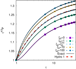
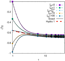
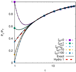
Figure 2: Comparison between the LB results obtained using $Q_{\xi}=20$ and the exact semi-analytic solution reported in Ref. [14] for $\xi_{0}\in\{0,1,\xi_{0}^{\rm H1},100\}$, where $\xi_{0}^{\rm H1}\simeq 2.67$ is obtained from Eq. (16), at $4\pi(\overline{\eta/s})=1$.

The conservation of the stress-energy tensor $\nabla_{\hat{\beta}}T^{{\hat{\alpha}}{\hat{\beta}}}$ reduces for the Bjorken flow to $3\tau\partial_{\tau}P+4P+\Pi=0$. In the first-order hydrodynamics theory, $\Pi=-\frac{4\eta}{3\tau}=-\frac{16\tau_{\rm A-W;0}}{15\tau}P^{3/4}$ where $\eta=\frac{4}{5}\tau_{\rm A-W}P$ is the Chapman-Enskog value for the shear viscosity [21]. In the second-order hydrodynamics theory, the constitutive equation for $\Pi$ is promoted to an evolution equation [12, 17]. It can be seen that in the first order theory, $\Pi_{0}=-\frac{16}{15}\tau_{\rm A-W;0}$, which can only be achieved via the Romatschke-Strickland form (6) when $\tau_{\rm A-W;0}<\frac{15}{16}$. The value $\xi_{0}^{\rm H1}$ corresponding to this value is the solution of the following equation ($\widetilde{k}_{B}\widetilde{T}_{0}=600\ {\rm MeV}$, $\widetilde{c}\widetilde{\tau}_{0}=0.25\ {\rm fm}$):

$$1-\frac{3}{\xi_{0}^{\rm H1}}+\frac{6}{\xi_{0}^{\rm H1}+\sqrt{\xi_{0}^{\rm H1}}(\xi_{0}^{\rm H1}+1)\arctan\sqrt{\xi_{0}^{\rm H1}}}\simeq 0.558321\times 4\pi(\overline{\eta/s}).$$ (16)

It is thus natural to consider a comparison between the first- and second-order hydrodynamics for the case when $\Pi_{0}$ coincides in the two theories (i.e., $\xi_{0}=\xi_{0}^{\rm H1}$). Figure 1 shows that, quite remarkably, the first-order theory seems to be in better agreement with the numerical results obtained using the LB algorithm presented in the previous section for $4\pi(\overline{\eta/s})\in\{0.1,0.5,1,1.7\}$. It is particularly interesting to note that, at $4\pi(\overline{\eta/s})=1.7$, the late time evolution of $\Pi$ overlaps with the first-order prediction, while the second-order hydrodynamics result remains in visible disagreement even at $\tau=40$.

Next, Fig. 2 shows the effect of varying the initial anisotropy $\xi_{0}$ at $4\pi(\overline{\eta/s})=1$. It can be seen that at fixed proper time $\tau$, the pressure increases as $\xi_{0}$ is increased. The first order hydrodynamic prediction seems to be a late time hydrodynamic attractor for $\Pi$ and more strikingly for $\mathcal{P}_{L}/\mathcal{P}_{T}$.

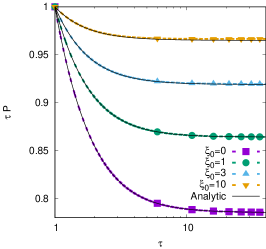
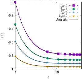
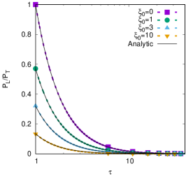
Figure 3: Comparison between LB results (lines and points) for the free-streaming case and the analytic solution (18) for various values of $\xi_{0}$.

In the free-streaming limit, $\tau_{\rm A-W;0}\rightarrow\infty$ and the right-hand side of Eq. (2) vanishes, such that:

$$f=\frac{1}{8\pi}\exp\left\{-\frac{p}{\Lambda_{0}}\sqrt{1+\xi^{2}[(1+\xi_{0})\tau^{2}-1]}\right\},$$ (17)

which corresponds to the following moments:

$$\mathcal{P}_{L,{\rm fs}} = \frac{3\Lambda_{0}^{4}}{2[(1+\xi_{0})\tau^{2}-1]}\left[\frac{\arctan{\sqrt{(1+\xi_{0})\tau^{2}-1}}}{\sqrt{(1+\xi_{0})\tau^{2}-1}}-\frac{1}{(1+\xi_{0})\tau^{2}}\right],$$

$$\mathcal{P}_{T,{\rm fs}} = \frac{3\Lambda_{0}^{4}}{4[(1+\xi_{0})\tau^{2}-1]}\left\{1+[(1+\xi_{0})\tau^{2}-2]\frac{\arctan{\sqrt{(1+\xi_{0})\tau^{2}-1}}}{\sqrt{(1+\xi_{0})\tau^{2}-1}}\right\}.$$ (18)

It can be seen in Fig. 3 that the numerical results obtained using $Q_{\xi}=40$ and $N_{\Omega}=6$ are in very good agreement with the above analytic results. The small discrepancy observed at $\xi_{0}=10$ becomes unnoticeable when $N_{\Omega}=8$.

5 CONCLUSIONS

In this paper, we developed a procedure to implement anisotropic initial conditions for the one-dimensional boost-invariant longitudinal expansion (Bjorken flow) in the frame of the lattice Boltzmann (LB) algorithm for the relativistic Boltzmann equation introduced in Ref. [17]. The accuracy of our implementation was demonstrated by comparison with the solutions of the first- and second-order hydrodynamics equations, with the analytic solution of the free streaming limit and with the semi-analytic solution derived in Ref. [14]. In all cases, an excellent agreement was found. The implementation of the initial anisotropy via an expansion of order $N_{\Omega}=6$ with respect to the Legendre polynomials of the Romatschke-Strickland form of the Maxwell-Jüttner distribution gave accurate results for $0\leq\xi_{0}\leq 100$ at finite values of $(\overline{\eta/s})$, however small deviations form the exact solution could be seen in the free-streaming limit for $\xi=10$. The accuracy of the simulations in this case can be improved by increasing $N_{\Omega}$.

When $\xi_{0}$ is used to set the initial value of the pressure deviator $\Pi_{0}$ to the value required by the first-order constitutive equations, our simulations show that the first-order theory remains in very good agreement with the numerical results even at $4\pi(\overline{\eta/s})=1.7$, where the second-order formulation is no longer accurate.

Increasing $\xi_{0}$ at fixed $4\pi(\overline{\eta/s})=1$, the initial pressure anisotropy can be directly controlled, with $\mathcal{P}_{L}/\mathcal{P}_{T}\rightarrow 0$ as $\xi_{0}\rightarrow\infty$. For all tested values of $\xi_{0}$, we found that $\mathcal{P}_{L}/\mathcal{P}_{T}$ converges to the same curve for $\tau\gtrsim 5$. In the future, we plan to analyse this result and compare with the hydrodynamic attractor solution proposed in Ref. [22]. Interestingly, $P$ (and hence $T=P^{1/4}$) seems to increase monotonically with $\xi_{0}$ when $\tau$ is kept fixed.

In the future, we plan to extend our LB algorithm to account for massive particles [23] and for particles obeying quantum (Fermi-Dirac and Bose-Einstein) statistics [24]. In the context of the Bjorken flow, our implementation can be validated against the semi-analytic solutions developed in Refs. [25] and [26], respectively.

ACKNOWLEDGMENTS. This work was supported by a grant of the Romanian Ministry of Research and Innovation, CCCDI-UEFISCDI, project number PN-III-P1-1.2-PCCDI-2017-0371, within PNCDI III.

References

• [1] W. Israel, Ann. Phys. 100, 310 (1976); W. Israel and J. M. Stewart, Ann. Phys. 118, 341 (1979).
• [2] C. L. Fryer, Stellar Collapse (Kluwer Academic Publishers, Dordrecht, Netherlands, 2004).
• [3] F. Banyuls, J. A. Font, J. M. Ibanez, J. M. Marti, and J. A. Miralles, Astrophys. J. 476, 221231 (1997).
• [4] G. F. R. Ellis, R. Maartens, and M. A. H. MacCallum, Relativistic cosmology (Cambridge University Press, Cambridge, UK, 2012).
• [5] B. V. Jacak and B. Muller, Science 337, 310314 (2012).
• [6] P. Romatschke and U. Romatschke, arXiv:1712.05815 [nucl-th].
• [7] B. Müller, “A New Phase of Matter: Quark-Gluon Plasma Beyond the Hagedorn Critical Temperature”, in Melting hadrons, boiling quarks, edited by J. Rafelski (Springer, 2015), DOI: 10.1007/978-3-319-17545-4, pp. 107–116.
• [8] J. D. Bjorken, Phys. Rev. D 27, 140–151 (1983).
• [9] P. Kovtun, D. T. Son, and A. O. Starinets, Phys. Rev. Lett. 94, 111601 (2005).
• [10] P. Romatschke and U. Romatschke, Phys. Rev. Lett. 99, 172301 (2007).
• [11] W. A. Hiscock and L. Lindblom, Ann. Phys. 151, 466–496 (1983).
• [12] A. Jaiswal, Phys. Rev. C 87, 051901 (2013).
• [13] C. Chattopadhyay, A. Jaiswal, S. Pal, and R. Ryblewski, Phys. Rev. C 91, 024917 (2015).
• [14] W. Florkowski, R. Ryblewski, and M. Strickland, Phys. Rev. C 88, 024903 (2013).
• [15] R. Baier and P. Romatschke, Eur. Phys. J. C 51, 677–687 (2007).
• [16] P. Romatschke, M. Mendoza, and S. Succi, Phys. Rev. C 84, 034903 (2011).
• [17] V. E. Ambru\cbs and R. Blaga, Phys. Rev. C 98, 035201 (2018).
• [18] P. Romatschke and M. Strickland, Phys. Rev. D 68, 036004 (2003).
• [19] C. Y. Cardall, E. Endeve, and A. Mezzacappa, Phys. Rev. D 88, 023011 (2013).
• [20] C.-W. Shu and S. Osher, J. Comput. Phys. 77, 439–471 (1988).
• [21] C. Cercignani and G. M. Kremer, The relativistic Boltzmann equation: theory and applications (Birkhäuser Verlag, Basel, Switzerland, 2002).
• [22] P. Romatschke, J. High Energy Phys. 12 (2017) 079.
• [23] A. Gabbana, M. Mendoza, S. Succi, and R. Tripiccione, Phys. Rev. E 95, 053304 (2017).
• [24] R. C. V. Coelho, M. Mendoza, M. M. Doria, and H. J. Herrmann, Comput. Fluids 172, 318–331 (2018).
• [25] W. Florkowski, E. Maksymiuk, R. Ryblewski, and M. Strickland, Phys. Rev. C 89, 054908 (2014).
• [26] W. Florkowski and E. Maksymiuk, J. Phys. G: Nucl. Part. Phys. 42, 045106 (2015).