Interacting particles with Lévy strategies: limits of transport equations for swarm robotic systems G. E. R. was supported by The Maxwell Institute Graduate School in Analysis and its Applications, a Centre for Doctoral Training funded by the UK Engineering and Physical Sciences Research Council (grant EP/L016508/01), the Scottish Funding Council, Heriot-Watt University and the University of Edinburgh.

Abstract

Lévy robotic systems combine superdiffusive random movement with emergent collective behaviour from local communication and alignment in order to find rare targets or track objects. In this article we derive macroscopic fractional PDE descriptions from the movement strategies of the individual robots. Starting from a kinetic equation which describes the movement of robots based on alignment, collisions and occasional long distance runs according to a Lévy distribution, we obtain a system of evolution equations for the fractional diffusion for long times. We show that the system allows efficient parameter studies for a search problem, addressing basic questions like the optimal number of robots needed to cover an area in a certain time. For shorter times, in the hyperbolic limit of the kinetic equation, the PDE model is dominated by alignment, irrespective of the long range movement. This is in agreement with previous results in swarming of self-propelled particles. The article indicates the novel and quantitative modeling opportunities which swarm robotic systems provide for the study of both emergent collective behaviour and anomalous diffusion, on the respective time scales.

92C17, 35R11, 35Q92, 35F20

1 Introduction

The automated searching of an area for a rare target and tracking are problems of long history in different areas of computer science [8]. They include search and rescue operations in disaster regions [31], exploration for natural resources, environmental monitoring [54] and surveillance. Systems of mobile robots have inherent advantages for these applications, compared to a single robot: the parallel and spatially distributed execution of tasks gives rise to larger sensing capabilities and efficient, fault tolerant strategies. See [50] for a review of recent advances on swarm robotics and applications.

In this article we consider macroscopic PDE descriptions applicable to swarm robotic systems, which achieve scalability for a large number of independent, simple robots based on local communication and emergent collective behaviour. Much of the research focuses on determining control laws of the robot movement which give rise to a desired group behavior [5], like a prescribed spatial distribution. Typical control laws like biased random walks, reaction to chemotactic cues and long range coordination, are reminiscent of models for biological systems, and many bio-inspired strategies have been implemented in robots in recent years, for a review see [46].

Of particular recent interest have been strategies which include nonlocal random movements beyond Brownian motion, leading to Lévy robotics [34]. Lévy walks, with the characteristic high number of long runs, minimize the expected hitting time to reach an unknown target. These new search strategies are inspired by nonlocal movement found in a variety of organisms like T cells [28], E. coli bacteria [33], mussels [10] and spider monkeys [44]. Conversely, robotic systems provide controlled, quantitative models rarely available in biology.

Given sets of control laws are assessed and optimized by expensive particle based simulations and experiments with robots, based on a wide range of quality metrics [2, 5, 57]. On the other hand, for biological systems effective macroscopic PDE descriptions have proven to be a key tool for efficient parameter optimization and analytical understanding. A series of studies dating to Patlak [42] has generated solid understanding on how microscopic detail translates into a diffusion-advection type equation [3, 56] for random walks subject to an external bias and interactions. Recent work has made progress towards nonlocal PDE descriptions of Lévy movement [21, 43, 52]. Emergence of superdiffusion without Lévy movement is discussed in [23].

In this article, motivated by the necessity of optimal search strategies for a swarm of robots, we study a system of $N$ individuals undergoing a velocity jump process with contact interactions and where the individuals align with their neighbors. We assume quasi-static behavior, i.e., along a single run changes in time of the robotic parameters are negligible, and use the molecular chaos assumption, that the velocity of particles which are about to collide is approximately uncorrelated. In a mean-field limit for $N\to\infty$, we obtain a system of fractional PDEs for the macroscopic density $u(\mathbf{x},t)$ and mean direction $w(\mathbf{x},t)$:

(1) $$\partial_{t}u+\nabla\cdot w =0\ ,$$

$$w-\ell\frac{G(u)}{F(u)}\Lambda^{w} =-\frac{1}{F(u)}C_{\alpha}\nabla^{\alpha-1}u\ ,$$

both assumed to be sufficiently smooth and integrable in $\mathds{R}^{n}$. Here $\Lambda^{w}$ is given by Eq. 43 and $F(u)$, $G(u)$ and the diffusion constant $C_{\alpha}$ are defined in defined by Eq. 50 and Eq. 51 respectively. The parameter $\ell$ gives the strength of the alignment. Starting from a kinetic equation that describes the movement of the individuals, combining short range interactions and alignment with occasional long runs, according to an approximate Lévy distribution, we obtain the system Eq. 1 in the appropriate parabolic time scale.

While diffusive behavior dominates for long times, swarming on shorter hyperbolic time scales is not affected by the Lévy movement, so that a rich body of work such as [4] on swarming applies to Lévy robotics. Combining long range dispersal and alignment as in the kinetic equation for the macroscopic density Eq. 30, allows us to obtain either a space fractional diffusion equation for a pure nonlocal movement of the individuals (see [21]), or a Vicsek-type equation for the case of pure alignment [11, 55].

To illustrate applications of the PDE description, Section 8 presents efficient numerical methods for the solution of Eq. 1 and applies them for some first parameter studies in the case of a search example. Detailed robotic studies of search strategies and targeting efficiency, based on (1), as well as comparisons to both standard particle simulations and experiments with E-Puck robots and drones are pursued in [18].

Concerning previous experimental work, the particular Lévy strategy considered here, with additional long waiting times during reorientations, was implemented in a swarm robotic system of iAnt robots to find targets in [25], while [49] combined a Lévy walk search strategy with an added repulsion among the robots. Lévy movement directed by external cues, such as chemotaxis, has been studied in [41] to find a contaminant in water, while [38] considers sonotaxis. Efficient spatial coverage in the presence of pheromone cues was specifically addressed in [45], using an ant-inspired search strategy with long range movement.

Notation: The words particles and individuals are used interchangibly in this work. We denote the unit sphere in $\mathbb{R}^{n}$ by $S=\{x\in\mathbb{R}^{n}:|x|=1\}$, its surface area by $|S|$.

2 Model assumptions

A swarm robotic system [46] consists of a large number of simple independent robots with local rules, communication and interactions among them and with the environment, where the local interactions may lead to collective behaviour of the swarm. A system of E-Puck robots [36] in a domain in $\mathbb{R}^{2}$ provides a specific model system, to which we apply our results and present numerical experiments in Section 8. More generally, we consider $N$ identical spherical individuals of diameter $\varrho>0$ in $\mathds{R}^{n}$, where $n=2,3$. Each individual is characterized by its position $\mathbf{x}_{i}\in\mathds{R}^{n}$ and direction $\mathbf{\theta}_{i}\in S=\{|\mathbf{x}_{i}|=1\}\subseteq\mathds{R}^{n}$. We assume that each individual moves according to the following rules:

1. Starting at position $\mathbf{x}$ at time $t$, an individual runs in direction $\theta$ for a Lévy distributed time $\tau$, called the “run time”.

2. The individuals move according to a velocity jump process with constant forward speed $c$, following a straight line motion interrupted by reorientation.

3. When the individual stops, with probability $\zeta$ it starts a long range run and tumble process, choosing a new direction $\theta^{*}$ according to a distribution $k(\mathbf{x},t,\mathbf{\theta};\mathbf{\theta}^{*})$. With probability $(1-\zeta)$ it aligns with the neighbors in a certain region.

4. When two individuals get close to each other they reflect elastically; the new direction is $\theta^{\prime}=\theta-2(\theta\cdot\nu)\nu$, where $\nu=\frac{\mathbf{x}_{i}-\mathbf{x}_{j}}{|\mathbf{x}_{i}-\mathbf{x}_{j}|}$ is the normal vector at the point of collision.

5. All reorientations are assumed to be instantaneous.

6. The running probability $\psi$, which is defined as the probability that an individual moving in some fixed direction does not stop until time $\tau$, is taken to be independent on the environment surrounding the individual.

Note that the assumptions correspond to independent individuals with simple capabilities relative to typical tasks for swarm robotic systems. They interact only with their neighbors in a fixed sensing region, and the movement decisions are based on the current positions and velocities, not information from earlier times. This assures the scalability to large numbers of robots, while nonlocal collective movement may emerge from the local rules [46].

Related movement laws have been used for target search, for example, in the experiments in [25]. Refined local control laws and the possibility for quantitative experiments with robots open up novel modeling opportunities, see Section 9.

3 Kinetic equation for microscopic movement

For the system of $N$ individuals moving on the trajectories $\{\mathbf{X}_{i}(t)\}_{i=1}^{N}$ described in Section 2, let us denote by $\sigma=\sigma(\mathbf{x}_{i},t,\theta_{i},\tau_{i})$ the $N$-particle probability density function. This means that the probability density of finding the individuals at time $t$ at position $\mathbf{x}_{i}$ moving in direction $\theta_{i}$ with run time $\tau_{i}$ is given by $\sigma(\mathbf{x}_{i},t,\theta_{i},\tau_{i})\prod_{i=1}^{N}d\mathbf{x}_{i}\ d\theta_{i}\ d\tau_{i}$. At least formally one expects that $\sigma$ evolves according to the kinetic equation given by [32]

(2) $$\partial_{t}\sigma+\sum_{i=1}^{N}\left(\partial_{\tau_{i}}+{\color[rgb]{0,0,0}c}\theta_{i}\cdot\nabla_{\mathbf{x}_{i}}\right)\sigma=-\sum_{i=1}^{N}\beta_{i}\sigma\ ,$$

in the domain $\Omega^{N}=\{(\mathbf{x}_{1},...,\mathbf{x}_{N})\in\mathds{R}^{n\times N}:\ |\mathbf{x}_{i}-\mathbf{x}_{j}|\geq\varrho\ \forall i,j\}$. The tumbling Eq. 5 and the alignment Eq. 6 described below determine the initial condition for the kinetic equation Eq. 2 at $\tau_{i}=0$ in Eq. 9 such that mass is conserved. The equation is complemented by an initial condition at time $t=0$ (smooth, compactly supported) and boundary conditions at $\partial\Omega^{N}$ corresponding to elastic collisions.

The stopping frequency $\beta_{i}$ during a run phase relates to the probability $\psi_{i}$ that an individual does not stop for a time $\tau_{i}$. It is given by

(3) $$\psi_{i}(\mathbf{x}_{i},\tau_{i})=\left(\frac{{\color[rgb]{0,0,0}\varsigma_{0}(\mathbf{x}_{i})}}{{\color[rgb]{0,0,0}\varsigma_{0}(\mathbf{x}_{i}})+\tau_{i}}\right)^{\alpha},\ \alpha\in(1,2)\ .$$

This power law behaviour corresponds to the long tailed distribution of run times described in Assumption 1. in Section 2, instead of the Poisson process in classical velocity jump models [19, 39, 40]. As the speed $c$ of the runs is constant, the individuals perform occasional long jumps with a power-law distribution of run lengths. The stopping frequency is given by

(4) $$\beta_{i}(\mathbf{x}_{i},\tau_{i})=-\frac{\partial_{\tau_{i}}\psi_{i}}{\psi_{i}}=\frac{\varphi_{i}}{\psi_{i}}\ .$$

After stopping, according to Assumption 3 individuals choose a new direction of motion by either tumbling or alignment. With probability $\zeta\in[0,1]$ they choose a new direction according to the turning kernel $T_{i}$ given by

(5) $$T_{i}\phi(\theta_{i}^{*})=\int_{S}k(\mathbf{x}_{i},t,\mathbf{\theta}_{i};\mathbf{\theta}_{i}^{*})\phi(\theta_{i})d\theta_{i}\ ,$$

where the new direction $\theta_{i}^{*}$ is symmetrically distributed with respect to the previous direction $\theta_{i}$ according to the distribution $k(\mathbf{x}_{i},t,\mathbf{\theta}_{i};\mathbf{\theta}_{i}^{*})=\tilde{k}(\mathbf{x}_{i},t,|\theta_{i}^{*}-\theta_{i}|)$ [1]. Because $\tilde{k}$ is a probability distribution, it is normalized to $\int_{S}\tilde{k}(\mathbf{x}_{i},t,|\theta_{i}-e_{1}|)d\theta_{i}=1$ where $e_{1}=(1,0,...,0)$.

With probability $(1-\zeta)$ the new direction of motion is aligned with the direction of the neighbors according to a distribution $\Phi(\Lambda_{i}\cdot\theta_{i})$, with $\int_{S}\Phi(\Lambda_{i}\cdot\theta_{i})d\theta_{i}=1$. The average direction $\Lambda_{i}$ at $\mathbf{x}_{i}$ is defined in terms of the nonlocal flux $\mathcal{J}(\mathbf{x}_{i})$ [15],

(6) $$\Lambda_{i}(\mathbf{x}_{i},\theta_{i},t)=\frac{\mathcal{J}(\mathbf{x}_{i},t)}{|\mathcal{J}(\mathbf{x}_{i},t)|}\ ,\ \mathcal{J}(\mathbf{x}_{i},t)=\int_{\mathds{R}^{n}}\int_{S}K(|\mathbf{x}_{j}-\mathbf{x}_{i}|)p(\mathbf{x}_{j},t,\theta_{j})\theta_{j}d\mathbf{x}_{j}d\theta_{j}\ .$$

Here $K$ is a given influence kernel and $p$ is the density of individuals at $\mathbf{x}_{j}$ at time $t$, moving in the direction $\theta_{j}$ defined as (for $j=1$)

$$p(\mathbf{x}_{1},t,\theta_{1})=$$

$$\ \ \frac{1}{|S|^{N}}\int_{[0,t]^{N}}\int_{\Omega_{N-1}(\mathbf{x}_{1})}\int_{S^{N}}\sigma(\mathbf{x}_{1},\theta_{1},\tau_{1},\dots,\mathbf{x}_{N},\theta_{N},\tau_{N},t)d\theta_{2}d\mathbf{x}_{2}d\tau_{2}\dots d\theta_{N}d\mathbf{x}_{N}d\tau_{N}\ .$$

The integral is over the domain $\Omega_{N-1}(\mathbf{x}_{1}):=\{(\mathbf{x}_{2},\dots,\mathbf{x}_{N}):(\mathbf{x}_{1},\mathbf{x}_{2},\dots,\mathbf{x}_{N})\in\Omega^{N}\}$ accessible to individuals $2,\dots,N$. If the flux $\mathcal{J}(\mathbf{x}_{i},t)=0$, we assume then that $\Lambda_{i}(\mathbf{x}_{i},\theta_{i},t)$ takes the value $\theta_{i}$ [13]. In the rest of the paper this convention will be recalled by the dependence of $\Lambda_{i}$ on $\theta_{i}$.

4 Transport equation for the two-particle density

In the following we assume that $\sigma$ and its derivatives are smooth. As the initial condition at time $0$ is of compact support, $\sigma$ is of compact support for every fixed $t$. The description Eq. 2 of the $N$-particle problem a priori requires the understanding of collisions among the whole system of particles. In this article, however, we aim for a macroscopic description for low densities, as made precise by the scaling in Section 5. In this regime collisions of more than two individuals are neglected [6], and we truncate the hierarchy of equations by neglecting collisions of $3$ or more individuals and integrate out individuals $3,...,N$ from $\sigma$. The transport equation which describes the movement of two particles $\mathbf{x}_{1},\ \mathbf{x}_{2}\in\Omega^{2}$, is given by

(7) $$\partial_{\tau_{1}}\sigma+\partial_{\tau_{2}}\sigma+\partial_{t}\sigma+c\theta_{1}\cdot\nabla_{\mathbf{x}_{1}}\sigma+c\theta_{2}\cdot\nabla_{\mathbf{x}_{2}}\sigma=-(\beta_{1}+\beta_{2})\sigma\ .$$

Here $\sigma=\sigma(\mathbf{x}_{1},\mathbf{x}_{2},t,\theta_{1},\theta_{2},\tau_{1},\tau_{2})$ is the two-particle density function and we impose the boundary and initial conditions as for Eq. 2.

We first integrate with respect to $\tau_{1}$ and $\tau_{2}$ to get

$$\partial_{t}\tilde{\tilde{\sigma}}+c\theta_{1}\cdot\nabla_{\mathbf{x}_{1}}\tilde{\tilde{\sigma}} +c\theta_{2}\cdot\nabla_{\mathbf{x}_{2}}\tilde{\tilde{\sigma}}=-{\int_{0}^{t}\int_{0}^{t}\beta_{1}\sigma d\tau_{1}d\tau_{2}}{-\int_{0}^{t}\int_{0}^{t}\beta_{2}\sigma d\tau_{1}d\tau_{2}}$$

(8) $${\color[rgb]{0,0,0}+\tilde{\sigma}_{\tau_{1}}(\mathbf{x}_{1},\mathbf{x}_{2},t,\theta_{1},\theta_{2},\tau_{1}=0)+\tilde{\sigma}_{\tau_{2}}(\mathbf{x}_{1},\mathbf{x}_{2},t,\theta_{1},\theta_{2},\tau_{2}=0)}\ ,$$

for

$$\tilde{\tilde{\sigma}}(\mathbf{x}_{1},\mathbf{x}_{2},t,\theta_{1},\theta_{2})=\int_{0}^{t}\int_{0}^{t}\sigma d\tau_{1}d\tau_{2}\ ,\ \ \tilde{\sigma}_{\tau_{1}}(\mathbf{x}_{1},\mathbf{x}_{2},t,\theta_{1},\theta_{2},\tau_{1})=\int_{0}^{t}\sigma d\tau_{2}\ ,$$

and similarly for $\tilde{\sigma}_{\tau_{2}}$. The last two terms in Equation 8 come from applying the Fundamental Theorem of Calculus to $\int_{0}^{t}\partial_{\tau_{1}}\sigma d\tau_{1}$ and $\int_{0}^{t}\partial_{\tau_{2}}\sigma d\tau_{2}$.

After stopping with rate given by $\beta_{1}$, from Section 3, the initial condition for the new run of individual $1$ is given by

(9) $$\tilde{\sigma}_{\tau_{1}}(\mathbf{x}_{1},\mathbf{x}_{2},t,\theta_{1},\theta_{2},{\color[rgb]{0,0,0}\tau_{1}=0})=\int_{S}Q(\theta_{1},\theta_{1}^{*})\int_{0}^{t}\beta_{1}\tilde{\sigma}_{\tau_{1}}(\mathbf{x}_{1},\mathbf{x}_{2},t,\theta_{1}^{*},\theta_{2},\tau_{1})d\tau_{1}d\theta_{1}^{*}\ ,$$

where

(10) $$Q(\theta_{1},\theta_{1}^{*})=\zeta k(\mathbf{x}_{1},t,\theta_{1}^{*};\theta_{1})+(1-\zeta)\Phi(\Lambda_{1}\cdot\theta_{1})\ .$$

The operator $Q(\theta_{1},\theta_{1}^{*})$ satisfies Assumption 3. from Section 2. In absence of collisions and for $\zeta=0$ we recover the kinetic equation for alignment interactions as in [12, 15, 27], while for $\zeta=1$ we obtain the long range velocity jump process from [21]. Substituting Eq. 9 and its analogue for individual 2 into the kinetic equation for $\tilde{\tilde{\sigma}}$, we obtain

(11) $$\underset{(\textnormal{\@slowromancap i@})}{\underbrace{\partial_{t}\tilde{\tilde{\sigma}}}} +\underset{(\textnormal{\@slowromancap ii@})}{\underbrace{c\theta_{1}\cdot\nabla_{\mathbf{x}_{1}}\tilde{\tilde{\sigma}}}}+\underset{(\textnormal{\@slowromancap iii@})}{\underbrace{c\theta_{2}\cdot\nabla_{\mathbf{x}_{2}}\tilde{\tilde{\sigma}}}}=-\underset{(\textnormal{\@slowromancap iv@})}{\underbrace{(\mathds{1}-\zeta T_{1})\int_{0}^{t}\int_{0}^{t}\beta_{1}\sigma d\tau_{1}d\tau_{2}}}$$

$$-\underset{(\textnormal{\@slowromancap v@})}{\underbrace{(\mathds{1}-\zeta T_{2})\int_{0}^{t}\int_{0}^{t}\beta_{2}\sigma d\tau_{1}d\tau_{2}}}+\underset{(\textnormal{\@slowromancap vi@})}{\underbrace{(1-\zeta)|S|\Phi(\Lambda_{1}\cdot\theta_{1})\int_{0}^{t}\beta_{1}P_{1}d\tau_{1}}}$$

$$+\underset{(\textnormal{\@slowromancap vii@})}{\underbrace{(1-\zeta)|S|\Phi(\Lambda_{2}\cdot\theta_{2})\int_{0}^{t}\beta_{2}P_{2}d\tau_{2}}}\ .$$

where

$$P_{1}(\mathbf{x}_{1},\mathbf{x}_{2},t,\theta_{2},\tau_{1})=\frac{1}{|S|}\int_{S}\tilde{\sigma}_{\tau_{1}}(\mathbf{x}_{1},\mathbf{x}_{2},t,\theta_{1}^{*},\theta_{2},\tau_{1})d\theta_{1}^{*}$$

and $P_{2}$ is similarly defined. Here $|S|$ denotes the surface area of the unit sphere $S$.

From the method of characteristics, we note that the solution of Eq. 7 is

(12) $$\sigma=\sigma_{0}(\mathbf{x}_{1}-c\theta_{1}\tau_{1},\mathbf{x}_{2}-c\theta_{2}\tau_{1},t-\tau_{1},\theta_{1},\theta_{2},0,\tau_{2}-\tau_{1})\psi_{1}(\mathbf{x}_{1},\tau_{1})\frac{\psi_{2}(\mathbf{x}_{2},\tau_{2})}{\psi_{2}(\mathbf{x}_{2},\tau_{2}-\tau_{1})}\ .$$

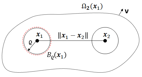
Figure 1: Illustration of the collision domain between two individuals.

From equation Eq. 11 for the two-particle density function $\tilde{\tilde{\sigma}}$ we now aim to derive an effective transport equation for the one-particle density function

(13) $$p(\mathbf{x}_{1},t,\theta_{1})=\frac{1}{|S|}\int_{0}^{t}\int_{0}^{t}\int_{\Omega_{2}}\int_{S}\sigma d\theta_{2}d\mathbf{x}_{2}d\tau_{1}d\tau_{2}\ .$$

By integrating equation Eq. 11 with respect to the accessible phase space $(\mathbf{x}_{2},\theta_{2})\in\Omega_{2}\times S$, where $\Omega_{2}=\Omega_{2}(\mathbf{x}_{1})=\{\mathbf{x}_{2}\in\mathds{R}^{n}:\ |\mathbf{x}_{1}-\mathbf{x}_{2}|>\varrho\}=\mathbb{R}^{n}\setminus B_{\varrho}(\mathbf{x}_{1})$ as in Figure 1, we obtain the following terms:

(i@) From our assumptions we commute the integrals and the time derivative, resulting in

$$\int_{\Omega_{2}}\int_{S}\partial_{t}\tilde{\tilde{\sigma}}d\theta_{2}d\mathbf{x}_{2}=|S|\partial_{t}p\ .$$

(ii@) From Reynolds’ transport theorem in the variable $\mathbf{x}_{1}$

$$c\int_{\Omega_{2}}\int_{S}\theta_{1}\cdot\nabla_{\mathbf{x}_{1}}\tilde{\tilde{\sigma}}d\theta_{2}d\mathbf{x}_{2}=|S|c\theta_{1}\cdot\nabla_{\mathbf{x}_{1}}p-c\int_{\partial B_{\varrho}(\mathbf{x}_{1})}\int_{S}(\theta_{1}\cdot\nu)\tilde{\tilde{\sigma}}d\theta_{2}d\mathbf{x}_{2}\ .$$

$\nu$ is the outward pointing unit normal vector with respect to $\Omega_{2}$.

(iii@) From the divergence theorem

$$c\int_{\Omega_{2}}\int_{S}\theta_{2}\cdot\nabla_{\mathbf{x}_{2}}\tilde{\tilde{\sigma}}d\theta_{2}d\mathbf{x}_{2} =c\int_{\partial B_{\varrho}}\int_{S}(\theta_{2}\cdot\nu)\tilde{\tilde{\sigma}}d\theta_{2}d\mathbf{x}_{2}\ ,$$

as $\tilde{\tilde{\sigma}}$ has compact support.

(iv@) Changing the order of integration we have

$$(\mathds{1}-\zeta T_{1}) \int_{\Omega_{2}}\int_{S}\int_{0}^{t}\int_{0}^{t}\beta_{1}(\mathbf{x}_{1},\tau_{1})\sigma(\mathbf{x}_{1},\mathbf{x}_{2},t,\theta_{1},\theta_{2},\tau_{1},\tau_{2})d\tau_{1}d\tau_{2}d\theta_{2}d\mathbf{x}_{2}$$

$$=|S|(\mathds{1}-\zeta T_{1})\int_{0}^{t}\beta_{1}(\mathbf{x}_{1},\tau_{1})J_{1}(\mathbf{x}_{1},t,\theta_{1},\tau_{1})d\tau_{1}\ ,$$

for $J_{1}(\mathbf{x}_{1},t,\theta_{1},\tau_{1})=\int_{\Omega_{2}}\int_{S}\int_{0}^{t}\sigma(\mathbf{x}_{1},\mathbf{x}_{2},t,\theta_{1},\theta_{2},\tau_{1},\tau_{2})d\tau_{2}d\theta_{2}d\mathbf{x}_{2}$.

(v@) Similar to (iv@) and using

$$\int_{S}T\phi(\cdot,\theta)d\theta=\int_{S}\phi(\cdot,\eta)\int_{S}k(\cdot,\eta;\theta)d\theta d\eta=\int_{S}\phi(\cdot,\eta)d\eta=\phi(\cdot)\ ,$$

where $\phi$ is an arbitrary function, we obtain

$$\int_{\Omega_{2}}\int_{S}(\mathds{1} -\zeta T_{2})\int_{0}^{t}\int_{0}^{t}\beta_{2}(\mathbf{x}_{2},\tau_{2})\sigma(\mathbf{x}_{1},\mathbf{x}_{2},t,\theta_{1},\theta_{2},\tau_{1},\tau_{2})d\tau_{1}d\tau_{2}\theta_{2}d\mathbf{x}_{2}$$

$$=|S|(1-\zeta)\int_{\Omega_{2}}\int_{0}^{t}\beta_{2}(\mathbf{x}_{2},\tau_{2})P_{2}(\mathbf{x}_{1},\mathbf{x}_{2},t,\theta_{1},\tau_{2})d\tau_{2}d\mathbf{x}_{2}\ .$$

(vi@) Moreover,

$$(1-\zeta)|S|\Phi(\Lambda_{1}\cdot\theta_{1}) \int_{S}\int_{\Omega_{2}}\int_{0}^{t}\beta_{1}(\mathbf{x}_{1},\tau_{1})P_{1}(\mathbf{x}_{1},\mathbf{x}_{2},t,\theta_{2},\tau_{1})d\tau_{1}d\mathbf{x}_{2}d\theta_{2}$$

$$=|S|^{2}(1-\zeta)\Phi(\Lambda_{1}\cdot\theta_{1})\int_{0}^{t}\beta_{1}(\mathbf{x}_{1},\tau_{1})\bar{P}_{1}(\mathbf{x}_{1},t,\tau_{1})d\tau_{1}\ ,$$

where $\bar{P}_{1}(\mathbf{x}_{1},t,\tau_{1})=|S|^{-1}\int_{\Omega_{2}}\int_{S}P_{1}(\mathbf{x}_{1},\mathbf{x}_{2},t,\theta_{2},\tau_{1})d\theta_{2}d\mathbf{x}_{2}$.

(vii@) Recalling the normalization $\int_{S}\Phi(\Lambda_{2}\cdot\theta_{2})d\theta_{2}=1$, we conclude

$$(1-\zeta)|S| \int_{S}\Phi(\Lambda_{2}\cdot\theta_{2})\int_{\Omega_{2}}\int_{0}^{t}\beta_{2}(\mathbf{x}_{2},\tau_{2})P_{2}(\mathbf{x}_{1},\mathbf{x}_{2},t,\theta_{1},\tau_{2})d\tau_{2}d\mathbf{x}_{2}d\theta_{2}$$

$$=|S|(1-\zeta)\int_{\Omega_{2}}\int_{0}^{t}\beta_{2}(\mathbf{x}_{2},\tau_{2})P_{2}(\mathbf{x}_{1},\mathbf{x}_{2},t,\theta_{1},\tau_{2})d\tau_{2}d\mathbf{x}_{2}\ .$$

From the above analysis we see that (v@) and (vii@) cancel. The final step now is to write (iv@) and (vi@) in terms of the density $p(\mathbf{x}_{1},t,\theta_{1})$ defined in Eq. 13. We proceed as follows.

From (iv@) and using the solution Eq. 12 we can write the integral as

$$\int_{0}^{t} \beta_{1}(\mathbf{x}_{1},\tau_{1})J_{1}(\mathbf{x}_{1},t,\theta_{1},\tau_{1})d\tau_{1}$$

$$=\int_{0}^{t}\int_{0}^{t}\varphi_{1}(\mathbf{x}_{1},\tau_{1})\bar{\sigma}_{0}(\mathbf{x}_{1}-c\theta_{1}\tau_{1},t-\tau_{1},\theta_{1},0,\tau_{2}-\tau_{1})\frac{\psi_{2}(\mathbf{x}_{2},\tau_{2})}{\psi_{2}(\mathbf{x}_{2},\tau_{2}-\tau_{1})}d\tau_{1}d\tau_{2}$$

(14) $$=\int_{0}^{t}\varphi_{1}(\mathbf{x}_{1},\tau_{1})\bar{\bar{\sigma}}_{0}(\mathbf{x}_{1}-c\theta_{1}\tau_{1},t-\tau_{1},\theta_{1},0)d\tau_{1}\ ,$$

where we have used $\frac{\psi_{2}(\mathbf{x}_{2},\tau_{2})}{\psi_{2}(\mathbf{x}_{2},\tau_{2}-\tau_{1})}\rightarrow 1$ for $\tau_{1}\ll 1$, i.e. we assume the trajectories of particle one are very short in time. From the definition Eq. 13 and using Eq. 12 again we write

(15) $$p(\mathbf{x}_{1},t,\theta_{1})=\int_{0}^{t}\bar{\bar{\sigma}}_{0}(\mathbf{x}_{1}-c\theta_{1}\tau_{1},t-\tau_{1},\theta_{1},0)\psi_{1}(\mathbf{x}_{1},\tau_{1})d\tau_{1}\ .$$

The standard arguments used in [21] allow to write Eq. 14 as a convolution by using the Laplace transform of Eq. 14 and Eq. 15 as follows,

(16) $$\int_{0}^{t}\beta_{1}(\mathbf{x}_{1},\tau_{1})J_{1}(\mathbf{x}_{1},t,\theta_{1},\tau_{1})d\tau_{1}=\int_{0}^{t}\mathcal{B}(\mathbf{x}_{1},t-s)p(\mathbf{x}_{1}-c\theta_{1}(t-s),s,\theta_{1})ds.$$

Here the operator $\mathcal{B}$ is defined from its Laplace transform $\hat{\mathcal{B}}=\mathcal{L}\{\mathcal{B}\}$ in time,

(17) $$\hat{\mathcal{B}}(\mathbf{x}_{1},\lambda+c\theta_{1}\cdot\nabla_{\mathbf{x}_{1}})=\frac{\hat{\varphi}_{1}(\mathbf{x}_{1},\lambda+c\theta_{1}\cdot\nabla_{\mathbf{x}_{1}})}{\hat{\psi}_{1}(\mathbf{x}_{1},\lambda+c\theta_{1}\cdot\nabla_{\mathbf{x}_{1}})}\ ,$$

with $\varphi_{1}$ and $\psi_{1}$ from Eq. 4. Explicit expressions for $\hat{\varphi}_{1}$ and $\hat{\psi}_{1}$ are found below in Section 6.

Following the same arguments we can write the integral in (vi@) as follows

(18) $$\int_{0}^{t}\beta_{1}(\mathbf{x}_{1},\tau_{1})\bar{P}_{1}(\mathbf{x}_{1},t,\tau_{1})d\tau_{1}=\int_{0}^{t}\mathcal{B}(\mathbf{x}_{1},t-s)u(\mathbf{x}_{1},s)ds\ ,$$

where $u(\mathbf{x}_{1},t)$ is a macroscopic density defined as

(19) $$u(\mathbf{x}_{1},t)=\int_{S}p(\mathbf{x}_{1},t,\theta_{1})d\theta_{1}\ .$$

Finally, including the results obtained in (i@)-(iii@) and the convolutions Eq. 15 and Eq. 18 we obtain

(20) $$\partial_{t}p+c\theta_{1}\cdot\nabla p =c|S|^{-1}\int_{\partial B_{\varrho}}\int_{S}\nu\cdot(\theta_{1}-\theta_{2})\tilde{\tilde{\sigma}}d\theta_{2}d\mathbf{x}_{2}$$

$$\qquad+(1-\zeta)|S|\Phi(\Lambda_{1}\cdot\theta_{1})\int_{0}^{t}\mathcal{B}(\mathbf{x}_{1},t-s)u(\mathbf{x}_{1},s)ds$$

$$\qquad-(\mathds{1}-\zeta T_{1})\int_{0}^{t}\mathcal{B}(\mathbf{x}_{1},t-s)p(\mathbf{x}_{1}-c\theta_{1}(t-s),s,\theta_{1})ds\ .$$

To summarize, the transport equation Eq. 20 describes the evolution of the one-particle density function $p(\mathbf{x}_{1},t,\theta_{1})$. The three terms on the right hand side describe the collisions, the alignment and the long range velocity jump process, respectively.

For later convenience we rewrite the collision term $\int_{\partial B_{\varrho}}\int_{S}\nu\cdot(\theta_{1}-\theta_{2})\tilde{\tilde{\sigma}}d\theta_{2}d\mathbf{x}_{2}$ as in Appendix A. Summing over the $N-1$ individuals which individual $1$ can collide with, equation Eq. 20 turns into

(21) $$\partial_{t}p +c\theta_{1}\cdot\nabla_{\mathbf{x}_{1}}p=(1-\zeta)|S|\Phi(\Lambda_{1}\cdot\theta_{1})\int_{0}^{t}\mathcal{B}(\mathbf{x}_{1},t-s)u(\mathbf{x}_{1},s)ds$$

$$-(\mathds{1}-\zeta T_{1})\int_{0}^{t}\mathcal{B}(\mathbf{x}_{1},t-s)p(\mathbf{x}_{1}-c\theta_{1}(t-s),s,\theta_{1})ds$$

$$+|S|^{-1}c\varrho^{n-1}(N-1)\int_{S_{+}}\int_{S}\nu\cdot(\theta_{1}-\theta_{2})\Bigl{[}\tilde{\tilde{\sigma}}(\mathbf{x}_{1},\mathbf{x}_{1}-\nu\varrho,t,\theta_{1}^{\prime},\theta_{2}^{\prime})$$

$$-\tilde{\tilde{\sigma}}(\mathbf{x}_{1},\mathbf{x}_{1}+\nu\varrho,\theta_{1},\theta_{2})\Bigr{]}d\theta_{2}d\nu\ .$$

Note that under the molecular chaos assumption each of the $N-1$ possible collision partners contributes an identical collision term to (21), which is therefore multiplied by $N-1$. From now on we work with equation Eq. 21 which describes the evolution of the one-particle density $p$ in the system of $N$-particles.

5 Parabolic scaling

In applications, the mean run time $\bar{\tau}$ is often small compared with the macroscopic time scale $\mathcal{T}$, and we aim to study Eq. 21 for $\varepsilon=\nicefrac{{\bar{\tau}}}{{\mathcal{T}}}\ll 1$ [1]. Denoting a macroscopic length scale by $\mathcal{X}$ and $s=\frac{\mathcal{X}}{\mathcal{T}}$, we introduce normalized variables

$$\bar{t}=\frac{t}{\mathcal{T}},\ \bar{\mathbf{x}}=\frac{\mathbf{x}}{\mathcal{X}},\ \bar{\tau}=\frac{\tau}{\bar{\tau}}\ \mathrm{and}\ \bar{c}=\frac{c}{s}\ .$$

A diffusion limit of Eq. 21 is obtained under the scaling $(\mathbf{x},t,\tau)\mapsto(\bar{\mathbf{x}}s/\varepsilon,\thinspace\bar{t}/\varepsilon,\thinspace\bar{\tau}/\varepsilon^{\mu})$, with $\bar{c}=\varepsilon^{-\gamma}c_{0}$ for $\mu,\ \gamma>0$. We further assume that the diameter of each particle is small, $\varrho=\varepsilon^{\xi}$, while the number of particles $N$ is large so that $(N-1)\varrho=\varepsilon^{\xi-\vartheta}$, with $\xi-\vartheta<0$. The scaling of the alignment is $\varepsilon^{-\eta}$.

In the normalized variables equations Eq. 4 and Eq. 3 become, after dropping the bar for the new variables,

(22) $$\beta_{\varepsilon}(\mathbf{x}_{1},\tau_{1})=\frac{\alpha\varepsilon^{\mu}}{\varsigma_{0}\varepsilon^{\mu}+\tau_{1}},\ \ \psi_{\varepsilon}(\mathbf{x}_{1},\tau_{1})=\left(\frac{\varsigma_{0}\varepsilon^{\mu}}{\varsigma_{0}\varepsilon^{\mu}+\tau_{1}}\right)^{\alpha}\ .$$

Similarly, equation Eq. 21 now reads

(23) $$\varepsilon\partial_{t}p +\varepsilon^{1-\gamma}c_{0}\theta_{1}\cdot\nabla p=\varepsilon^{-\eta}(1-\zeta)|S|\Phi^{\varepsilon}(\Lambda_{1}\cdot\theta_{1})\int_{0}^{t}\mathcal{B}^{\varepsilon}(\mathbf{x}_{1},t-s)u(\mathbf{x}_{1},s)ds$$

$$-(\mathds{1}-\zeta T_{1})\int_{0}^{t}\mathcal{B}^{\varepsilon}(\mathbf{x}_{1},t-s)p(\mathbf{x}_{1}-c\theta_{1}(t-s),s,\theta_{1})ds$$

$$+\varepsilon^{\xi-\vartheta-\gamma}|S|^{-1}c_{0}\int_{S_{+}}\int_{S}\nu\cdot(\theta_{1}-\theta_{2})\Bigl{[}\tilde{\tilde{\sigma}}(\mathbf{x}_{1},\mathbf{x}_{1}-\varepsilon^{\xi}\nu,t,\theta_{1}^{\prime},\theta_{2}^{\prime})$$

$$-\tilde{\tilde{\sigma}}(\mathbf{x}_{1},\mathbf{x}_{1}+\varepsilon^{\xi}\nu,\theta_{1},\theta_{2})\Bigr{]}d\theta_{2}d\nu\ ,$$

in dimension $2$, where the operator in the second convolution is given by

(24) $$\hat{\mathcal{B}}^{\varepsilon}=\hat{\mathcal{B}}^{\varepsilon}(\mathbf{x}_{1},\varepsilon\lambda+\varepsilon^{1-\gamma}c_{0}\theta_{1}\cdot\nabla)=\frac{\hat{\varphi}_{1}^{\varepsilon}(\mathbf{x}_{1},\varepsilon\lambda+\varepsilon^{1-\gamma}c_{0}\theta_{1}\cdot\nabla)}{\hat{\psi}_{1}^{\varepsilon}(\mathbf{x}_{1},\varepsilon\lambda+\varepsilon^{1-\gamma}c_{0}\theta_{1}\cdot\nabla)}\ .$$

With the above scaling, we may further simplify the collision term. To do so we introduce the molecular chaos assumption, which is plausible at low density of particles [6, 24]. It states that the velocity of the individuals is approximately independent of each other, so that the two-particle density approximately factors into one-particle densities:

$$\tilde{\tilde{\sigma}}(\mathbf{x}_{1},\mathbf{x}_{1}\pm\varepsilon^{\xi}\nu,t,\theta_{1},\theta_{2})=p(\mathbf{x}_{1},t,\theta_{1})p(\mathbf{x}_{1},t,\theta_{2})+\mathcal{O}(\varepsilon^{\xi})\ .$$

This is a standard assumption in the derivation of the kinetic equation for the one-particle density and is assumed in the remainder of this article. See for instance [13, 24] and references therein. Expression Eq. 23 then becomes

(25) $$\varepsilon\partial_{t} p+\varepsilon^{1-\gamma}c_{0}\theta_{1}\cdot\nabla p=\varepsilon^{-\eta}(1-\zeta)|S|\Phi^{\varepsilon}(\Lambda_{1}\cdot\theta_{1})\int_{0}^{t}\mathcal{B}^{\varepsilon}(\mathbf{x}_{1},t-s)u(\mathbf{x}_{1},s)ds$$

$$-(\mathds{1}-\zeta T_{1})\int_{0}^{t}\mathcal{B}^{\varepsilon}(\mathbf{x}_{1},t-s)p(\mathbf{x}_{1}-c\theta_{1}(t-s),s,\theta_{1})ds$$

$$+\varepsilon^{\xi-\vartheta-\gamma}|S|^{-1}c_{0}\int_{S_{+}}\int_{S}\nu\cdot(\theta_{1}-\theta_{2})\Bigl{[}p(\theta_{1}^{\prime})p(\theta_{2}^{\prime})-p(\theta_{1})p(\theta_{2})\Bigr{]}d\theta_{2}d\nu\ .$$

6 Fractional diffusion equation

In the above parabolic scaling, this section obtains a fractional diffusion equation from Eq. 25 for the macroscopic density of individuals moving according to the model in Section 2.

Up to lower order terms, we expand $p(\mathbf{x}_{1},t,\theta_{1})$ in terms of its first two moments

(26) $$p(\mathbf{x}_{1},t,\theta_{1})=|S|^{-1}\left(u(\mathbf{x}_{1},t)+\varepsilon^{\gamma}n\theta_{1}\cdot w(\mathbf{x}_{1},t)+o(\varepsilon^{\gamma})\right)\ ,$$

where $u(\mathbf{x}_{1},t)$ is defined in Eq. 19 and

(27) $$w(\mathbf{x}_{1},t)=\int_{S}\theta_{1}p(\mathbf{x}_{1},t,\mathbf{\theta}_{1})d\theta_{1}\ .$$

Substituting Eq. 26 into Eq. 25 and integrating with respect to $\theta_{1}$, we obtain the conservation law for the macroscopic density:

(28) $$\varepsilon\partial_{t}u(\mathbf{x}_{1},t)+\varepsilon nc_{0}\nabla\cdot w(\mathbf{x}_{1},t)=0\ .$$

To see this, note that the integral over the right hand side of Eq. 25 vanishes: for the last term in Eq. 25 this is due to the symmetry in $\theta_{1}$ and $\theta_{2}$, while for the first two terms it follows from the normalization of $\Phi(\Lambda_{1}\cdot\theta_{1})$, resp. $T_{1}$, as in Section 4 above.

To complement Eq. 28, it remains to express $w$ in terms of $u$. To do so, we use a quasi-static approximation for the Laplace transform of Eq. 25,

(29) $$\hat{\mathcal{B}}^{\varepsilon}(\mathbf{x}_{1},\varepsilon\lambda+\varepsilon^{1-\gamma}c_{0}\theta_{1}\cdot\nabla)\simeq\hat{\mathcal{B}}^{\varepsilon}(\mathbf{x}_{1},\varepsilon^{1-\gamma}c_{0}\theta_{1}\cdot\nabla)\ ,$$

since $\gamma>0$. Transforming back we obtain

(30) $$\varepsilon\partial_{t} p+\varepsilon^{1-\gamma}c_{0}\theta_{1}\cdot\nabla p=\varepsilon^{-\eta}(1-\zeta)|S|\Phi^{\varepsilon}(\Lambda_{1}\cdot\theta_{1})\int_{0}^{t}\mathcal{B}^{\varepsilon}(\mathbf{x}_{1},t-s)u(\mathbf{x}_{1},s)ds$$

$$-(\mathds{1}-\zeta T_{1})\hat{\mathcal{B}}^{\varepsilon}(\mathbf{x}_{1},\varepsilon^{1-\gamma}c_{0}\theta_{1}\cdot\nabla)p$$

$$+|S|^{-1}c_{0}\varepsilon^{\xi-\vartheta-\gamma}\int_{S_{+}}\int_{S}\nu\cdot(\theta_{1}-\theta_{2})\Bigl{[}p(\theta_{1}^{\prime})p(\theta_{2}^{\prime})-p(\theta_{1})p(\theta_{2})\Bigr{]}d\theta_{2}d\nu\ .$$

Equation Eq. 24 allows to obtain an explicit expression for $\hat{\mathcal{B}}^{\varepsilon}(\mathbf{x}_{1},\varepsilon^{1-\gamma}c_{0}\theta_{1}\cdot\nabla)$, based on the Laplace transforms of $\psi_{1}^{\varepsilon}$ and $\varphi_{1}^{\varepsilon}$ [21]:

$$\hat{\psi}_{1}^{\varepsilon}(\mathbf{x}_{1},\lambda)=a^{\alpha}\lambda^{\alpha-1}e^{a\lambda}\Gamma(-\alpha+1,a\lambda)\ \ \textnormal{and}\ \ \hat{\varphi}_{1}^{\varepsilon}(\mathbf{x}_{1},\lambda)=\alpha(a\lambda)^{\alpha}\Gamma(-\alpha,a\lambda)e^{a\lambda}\ ,$$

where we use an asymptotic expansion for the incomplete Gamma function

(31) $$\Gamma(b,z) =\Gamma(b)\left(1-z^{b}e^{-z}\sum_{k=0}^{\infty}\frac{z^{k}}{\Gamma(b+k+1)}\right),$$

for $b$ positive and not integer [17].

Here $a=\varsigma_{0}\varepsilon^{\mu}$. We conclude

(32) $$\hat{\mathcal{B}}^{\varepsilon}(\mathbf{x}_{1},\lambda)=\frac{\hat{\varphi}_{1}^{\varepsilon}(\mathbf{x}_{1},\lambda)}{\hat{\psi}_{1}^{\varepsilon}(\mathbf{x}_{1},\lambda)}=\frac{\alpha-1}{a}-\frac{\lambda}{2-\alpha}-a^{\alpha-2}\lambda^{\alpha-1}(\alpha-1)^{2}\Gamma(-\alpha+1)+\mathcal{O}(a^{\alpha-1}\lambda^{\alpha})\ .$$

Equation Eq. 32 is the key ingredient to express $w$ in terms of $u$. First rewrite Eq. 30 as

(33) $$\varepsilon\partial_{t}p+\varepsilon^{1-\gamma}c_{0}\theta_{1}\cdot\nabla p=\varepsilon^{-\eta}M_{\varepsilon}+H_{\varepsilon}p+\varepsilon^{\xi-\vartheta-\gamma}|S|^{-1}c_{0}L_{\varepsilon}\ ,$$

where

(34) $$M_{\varepsilon} =(1-\zeta)|S|\Phi^{\varepsilon}(\Lambda_{1}\cdot\theta_{1})\int_{0}^{t}\mathcal{B}^{\varepsilon}(\mathbf{x}_{1},t-s)u(\mathbf{x}_{1},s)ds\ ,$$

(35) $$H_{\varepsilon} =-(\mathds{1}-\zeta T_{1})\hat{\mathcal{B}}^{\varepsilon}(\mathbf{x}_{1},\varepsilon^{1-\gamma}c_{0}\theta_{1}\cdot\nabla)\ \ \textnormal{and}$$

(36) $$L_{\varepsilon}=\int_{S_{+}}\int_{S}\nu\cdot(\theta_{1}-\theta_{2})\Bigl{[}p(\theta_{1}^{\prime})p(\theta_{2}^{\prime})-p(\theta_{1})p(\theta_{2})\Bigr{]}d\theta_{2}d\nu\ .$$

Substituting Eq. 26 into Eq. 33, multiplying by $\theta_{1}$ and integrating with respect to this variable, we see that

$$\varepsilon^{\gamma+1}n \partial_{t}w(\mathbf{x}_{1},t)+\varepsilon^{1-\gamma}c_{0}\nabla u(\mathbf{x}_{1},t)=\varepsilon^{-\eta}\int_{S}\theta_{1}M_{\varepsilon}d\theta_{1}$$

(37) $$+|S|^{-1}\int_{S}\theta_{1}H_{\varepsilon}(u(\mathbf{x}_{1},t)+\varepsilon^{\gamma}n\theta_{1}\cdot w(\mathbf{x}_{1},t))d\theta_{1}+|S|^{-1}\varepsilon^{\xi-\vartheta-\gamma}c_{0}\int_{S}\theta_{1}L_{\varepsilon}d\theta_{1}\ .$$

The following subsections compute the various terms on the right hand side of Eq. 37.

6.1 Collision interactions

The third term

$$I=\int_{S}\theta_{1}L_{\varepsilon}d\theta_{1} =\int_{S}\int_{S}\int_{S_{+}}\theta_{1}p(\mathbf{x}_{1},\theta_{1}^{\prime})p(\mathbf{x}_{1},\theta_{2}^{\prime})\nu\cdot(\theta_{1}-\theta_{2})d\nu d\theta_{1}d\theta_{2}$$

$$\qquad-\int_{S}\int_{S}\int_{S_{+}}\theta_{1}p(\mathbf{x}_{1},\theta_{1})p(\mathbf{x}_{1},\theta_{2})\nu\cdot(\theta_{1}-\theta_{2})d\nu d\theta_{1}d\theta_{2}\ .$$

may be treated similar to [24]. From the elastic reflection $\theta_{1}^{\prime}-\theta_{1}=-2(\theta_{1}\cdot\nu)\nu$ we note $\theta_{1}^{\prime}\cdot\nu=-\theta_{1}\cdot\nu$, so that

(38) $$I=\int_{S}\int_{S}\int_{S_{+}}(\theta_{1}^{\prime}-\theta_{1})p(\mathbf{x}_{1},\theta_{1})p(\mathbf{x}_{1},\theta_{2})(\theta_{1}-\theta_{2})\cdot\nu d\nu d\theta_{1}d\theta_{2}\ .$$

Using the reflection law again, we see for $n=2$

(39) $$I=-\frac{4}{3}\int_{S}\int_{S}|\theta_{1}-\theta_{2}|\theta_{1}p(\mathbf{x}_{1},\theta_{1})p(\mathbf{x}_{1},\theta_{2})d\theta_{1}d\theta_{2}\ .$$

With the expansion Eq. 26 for $p(\mathbf{x}_{1},t,\theta_{1})$ and,

$$p(\mathbf{x}_{1},t,\theta_{2})=|S|^{-1}(u(\mathbf{x}_{1},t)+2\varepsilon^{\gamma}\theta_{2}\cdot w(\mathbf{x}_{1},t))\ ,$$

we conclude from Eq. 39

$$I =-\frac{4}{3|S|}\int_{S}\int_{S}|\theta_{1}-\theta_{2}|\theta_{1}\Bigl{[}u^{2}+2u\varepsilon^{\gamma}\theta_{2}\cdot w+2u\varepsilon^{\gamma}\theta_{1}\cdot w\Bigr{]}d\theta_{1}d\theta_{2}{\color[rgb]{0,0,0}+\mathcal{O}(\varepsilon^{2\gamma})}$$

(40) $$=-\frac{8u\varepsilon^{\gamma}}{3|S|}\int_{S}\int_{S}|\theta_{1}-\theta_{2}|\theta_{1}(\theta_{2}\cdot w+\theta_{1}\cdot w)d\theta_{1}d\theta_{2}+\mathcal{O}(\varepsilon^{2\gamma})\ ,$$

since $\int_{S}\theta_{1}d\theta_{1}=0$. The integral in Eq. 40 can be computed:

$$\int_{S}(\theta_{2}\cdot w)\Bigl{[}\int_{S}|\theta_{1}-\theta_{2}|\theta_{1}d\theta_{1}\Bigr{]}d\theta_{2} +\int_{S}\theta_{1}(\theta_{1}\cdot w)\Bigl{[}\int_{S}|\theta_{1}-\theta_{2}|d\theta_{2}\Bigr{]}d\theta_{1}=0+bw\ .$$

Here we have used $\int_{S}|\theta_{1}-\theta_{2}|d\theta_{2}=b\ \ \textnormal{and}\ \ \int_{S}\theta_{1}(\theta_{1}\cdot w)d\theta_{1}=w\ .$ We conclude

(41) $$I=-\varepsilon^{\gamma}\frac{8b}{3|S|}uw\ .$$

A more general expression for the case $n=3$ can be written as $I=-\varepsilon^{\gamma}b_{n}|S|^{-1}uw$. Expression Eq. 37 is thus written in terms of the first particle only, and we drop the subscript from now on.

6.2 Alignment

To evaluate the first term on the right hand side of Eq. 37, we first compute the alignment vector. From the expressions for $\Lambda^{w}$ and $\mathcal{J}$ in Eq. 6 and the expansion Eq. 26, we have

(42) $$\mathcal{J}(\mathbf{x}_{1},t) =\frac{\varepsilon^{\gamma}n}{|S|}\int_{\mathbf{y}}K^{\varepsilon}\left(\frac{|\mathbf{y}-\mathbf{x}_{1}|}{\varepsilon}\right)w(\mathbf{y},t)d\mathbf{y}\ ,$$

and therefore

(43) $$\Lambda^{w}=\frac{\int_{\mathbf{y}}K^{\varepsilon}\left(\frac{|\mathbf{y}-\mathbf{x}_{1}|}{\varepsilon}\right)w(\mathbf{y},t)d\mathbf{y}}{|\int_{\mathbf{y}}K^{\varepsilon}\left(\frac{|\mathbf{y}-\mathbf{x}_{1}|}{\varepsilon}\right)w(\mathbf{y},t)d\mathbf{y}|}\ .$$

Note that as $\varepsilon\rightarrow 0$, $\Lambda^{w}$ becomes local. Now the Laplace transform of $M_{\varepsilon}$ from Eq. 34 is given by

$$\hat{M}_{\varepsilon} =(1-\zeta)|S|\Phi^{\varepsilon}(\Lambda^{w}\cdot\theta)\hat{\mathcal{B}}^{\varepsilon}(\mathbf{x},\varepsilon\lambda)\hat{u}(\mathbf{x},\lambda)=(1-\zeta)|S|\Phi^{\varepsilon}(\Lambda^{w}\cdot\theta)\frac{\hat{\varphi}^{\varepsilon}(\mathbf{x},\varepsilon\lambda)}{\hat{\psi}^{\varepsilon}(\mathbf{x},\varepsilon\lambda)}\hat{u}(\mathbf{x},\lambda)\ .$$

To leading order in $\varepsilon$ we therefore deduce from the expansion Eq. 32 that

$$M_{\varepsilon}\simeq(1-\zeta)|S|\Phi^{\varepsilon}(\Lambda^{w}\cdot\theta)\frac{\varepsilon^{-\mu}(\alpha-1)}{\varsigma_{0}}u(\mathbf{x},t)\ .$$

Integrating over the sphere, $\Psi^{\varepsilon}(\Lambda^{w})=\int_{S}\theta\Phi^{\varepsilon}(\Lambda^{w}\cdot\theta)d\theta=z\Lambda^{w}\ ,$ where $z$ is given by

(44) $$z=\int_{0}^{2\pi}\Phi^{\varepsilon}(\cos\theta)\cos\theta d\theta\ ,$$

we conclude

$$\varepsilon^{-\eta}\int_{S}\theta_{1}M_{\varepsilon}d\theta_{1}=\varepsilon^{-\mu-\eta}(1-\zeta)\frac{z(\alpha-1)}{\varsigma_{0}}u\Lambda^{w}\ .$$

6.3 Long range movement

The second term on the right hand side of Eq. 37 has been computed in [21]:

$$\frac{\varepsilon^{\frac{\gamma}{\alpha-1}-1}}{|S|}\int_{S}\theta H_{\varepsilon}(u+\varepsilon^{\gamma}n\theta\cdot w)d\theta\simeq$$

$$-\frac{\varsigma_{0}^{\alpha-2}}{|S|}(1-\alpha)^{2}\Gamma(-\alpha+1)c_{0}^{\alpha-1}\nabla^{\alpha-1}u\left(\frac{\zeta n^{2}\nu_{1}}{|S|}-1\right)+\frac{\alpha-1}{\varsigma_{0}|S|}nw(\zeta\nu_{1}-1)\ .$$

Here $\nu_{1}$ is the second eigenvalue of the operator $T_{1}$ [1]. Substituting the results of Section 6.1 and Section 6.2 into Eq. 37 results in

$$\varepsilon^{\gamma+1}n\partial_{t}w+{\color[rgb]{0,0,0}\varepsilon^{1-\gamma}}c_{0}\nabla u =\varepsilon^{-\mu-\eta}(1-\zeta)\frac{z(\alpha-1)}{\varsigma_{0}}u\Lambda^{w}$$

(45) $$\qquad+\frac{1}{|S|}\int_{S}\theta H_{\varepsilon}(u+\varepsilon^{\gamma}n\theta\cdot w)d\theta-\varepsilon^{\xi-\vartheta}\frac{4bc_{0}}{3|S|^{2}}nuw\ .$$

Furthermore, using Subsection 6.3 the term of order $\varepsilon^{1-\frac{\gamma}{\alpha-1}}$ is given by

$$0=-\frac{\varsigma_{0}^{\alpha-2}}{|S|}(1-\alpha)^{2}\Gamma(-\alpha+1)c_{0}^{\alpha-1} \nabla^{\alpha-1}u\left(\frac{\zeta n^{2}\nu_{1}}{|S|}-1\right)+\frac{\alpha-1}{\varsigma_{0}|S|}nw(\zeta\nu_{1}-1)$$

(46) $$-\frac{4bc_{0}}{3|S|^{2}}nuw+(1-\zeta)\frac{z(\alpha-1)}{\varsigma_{0}}u\Lambda^{w}$$

provided the following scaling relations are satisfied:

(47) $$\mu=\frac{1-\alpha(1-\gamma)}{\alpha-1},\ \ \eta=-\gamma,\ \ \textnormal{and}\ \ \xi-\vartheta=1-\frac{\gamma}{\alpha-1}<0\ .$$

Here $\gamma>(\alpha-1)/\alpha$ to guarantee that $\mu>0$ and $\xi-\vartheta<0$. This is in agreement with the assumption that $1-\gamma<1$ used in Section 6 for the quasi-static approximation in Eq. 29. As was assumed in Section 5, $\xi-\vartheta<0$ which implies that $(N-1)\varrho\rightarrow\infty$ as $\varepsilon\rightarrow 0$.

From Eq. 46 we obtain an expression for $w$ and conclude the following.

Theorem 6.1 (formal).

As $\varepsilon\rightarrow 0$, the first two moments of the solution to Eq. 33 satisfy the following fractional diffusion equation for the macroscopic density $u(\mathbf{x},t)$ and the mean direction $w(\mathbf{x},t)$:

(48) $$\partial_{t}u+\nabla\cdot w =0\ ,$$

(49) $$w-\ell\frac{G(u)}{F(u)}\bar{\Lambda}^{w} =-\frac{1}{F(u)}C_{\alpha}\nabla^{\alpha-1}u\ ,$$

where $\bar{\Lambda}^{w}=\lim_{\varepsilon\rightarrow 0}\Lambda^{w}$ for $\Lambda^{w}$ given by Eq. 43,

(50) $$F(u)=\frac{\alpha-1}{\varsigma_{0}|S|}n(1-\zeta\nu_{1})+\frac{8bc_{0}}{3|S|^{2}}u,\ \ G(u)=(1-\zeta)|S|\frac{z(\alpha-1)}{\varsigma_{0}}u$$

and

(51) $$C_{\alpha}=-\frac{\varsigma_{0}^{\alpha-2}c_{0}^{\alpha-1}(\alpha-1)^{2}\pi}{\sin(\pi\alpha)\Gamma(\alpha)}\frac{(|S|-4\zeta\nu_{1})}{|S|^{2}}\ .$$

Recall that the parameter $\ell$ in Eq. 49 describes the strength of the alignment.

Without alignment, $\zeta=1$, the term $G(u)$ vanishes and we recover the result in [21] in the absence of chemotaxis. Appendix B discusses two different types of alignment kernels and their effect on the dynamics of the system Eq. 48-Eq. 49.

7 Macroscopic transport equation for swarming

This section studies the PDE description of the robot movement on shorter, hyperbolic time scales, where the formation of patterns like swarming can be expected. For simplicity we neglect the collision interaction term proportional to $\varrho^{N-1}$ in Eq. 21, i.e., we consider non-interacting individuals. We compare the resulting description obtained here with some classical results in [13, 37].

The hyperbolic scaling limit obtained by setting $\gamma=0$ in Section 5, so that $\mathbf{x}_{n}=\varepsilon\mathbf{x}/s,\ t_{n}=\varepsilon t,\ \tau_{n}=\tau\varepsilon^{\mu}\ .$ The space and time variables are on the same scale, and the quasi-static approximation in Eq. 29 is no longer justified. The kinetic equation Eq. 21 for the microscopic particle movement is therefore given by

$$\varepsilon(\partial_{t}p+c_{0}\theta\cdot\nabla p) =(1-\zeta)|S|\Phi^{\varepsilon}(\Lambda_{1}\cdot\theta)\int_{0}^{t}\mathcal{B}^{\varepsilon}(\mathbf{x},t-s)u(\mathbf{x},s)ds$$

(52) $$\qquad-(\mathds{1}-\zeta T_{1})\int_{0}^{t}\mathcal{B}^{\varepsilon}(\mathbf{x},t-s)p(\mathbf{x}-c\theta(t-s),s,\theta)ds\ .$$

The Laplace transform of Eq. 52 is

$$\varepsilon(\lambda+c_{0}\theta\cdot\nabla)\hat{p}-\varepsilon p_{0}= (1-\zeta)|S|\Phi^{\varepsilon}(\Lambda_{1}\cdot\theta)\hat{\mathcal{B}}^{\varepsilon}(\mathbf{x},\varepsilon\lambda)\hat{u}(\mathbf{x},\lambda)$$

(53) $$-(\mathds{1}-\zeta T_{1})\hat{\mathcal{B}}^{\varepsilon}(\mathbf{x},\varepsilon\lambda+\varepsilon c_{0}\theta\cdot\nabla)\hat{p}\ ,$$

where from Eq. 32 the operator $\hat{\mathcal{B}}^{\varepsilon}$ takes the form

(54) $$\hat{\mathcal{B}}^{\varepsilon}(\mathbf{x} ,\varepsilon\lambda)=\varepsilon^{-\mu}A+\varepsilon^{\mu(\alpha-2)+\alpha-1}B\lambda^{\alpha-1}+\mathcal{O}(\varepsilon)\ ,$$

with

(55) $$A=\frac{\alpha-1}{\varsigma_{0}}\ \ \textnormal{and}\ \ B=-\varsigma_{0}^{\alpha-2}(\alpha-1)^{2}\Gamma(-\alpha+1)\ .$$

In order to obtain a conservation equation for the macroscopic density, we start from the generalized Chapman-Enskog expansion for $\hat{p}$ in Appendix C,

(56) $$\hat{p}(\mathbf{x},\lambda,\theta)=\Phi_{\varsigma}(\theta)\hat{u}+\varepsilon^{(\mu+1)(\alpha-1)}\hat{p}_{1}+\mathcal{O}(\varepsilon^{2(\mu+1)(\alpha-1)})\ ,$$

with $\hat{p}_{1}$ given by Eq. 76 and $\Phi_{\zeta}(\theta)=(1-\zeta)\Phi^{\varepsilon}(\Lambda_{1}\cdot\theta)+\zeta$. Substituting Eq. 56 into Eq. 52 and integrating over $S$, we obtain the conservation equation

(57) $$\partial_{t}u+zc_{0}(1-\zeta)\nabla\cdot(u\Lambda_{1})=0\ .$$

Note that the right hand side is zero by conservation of particles, as in Eq. 28.

It remains to determine the mean direction $u\Lambda$, and for simplicity we start from Eq. 53. Substituting the expansion Eq. 56 into Eq. 53, using the definitions of $\hat{p}_{0}$ and $\hat{p}_{1}$ given in Eq. 75 and Eq. 76 respectively, and expanding in powers of $\varepsilon$, we find

(58) $$(\lambda\Phi_{\zeta}\hat{u}+c_{0}\theta\cdot\nabla(\Phi_{\zeta}\hat{u}))-p_{0}+\varepsilon^{(\mu+1)(\alpha-1)}(\lambda\hat{p}_{1}+c_{0}\theta\cdot\nabla\hat{p}_{1})=\mathcal{O}(\varepsilon^{(\mu+1)(2\alpha-3)})\ .$$

We multiply Eq. 58 by $\theta\cdot v$, where $v\in\mathds{R}^{n}$ is orthogonal to $\Lambda_{1}$, and integrate over $S$,

$$\Bigl{[}\int_{S}\theta(\lambda\Phi_{\zeta}\hat{u} +c_{0}\theta\cdot\nabla(\Phi_{\zeta}\hat{u}))d\theta-\int_{S}\theta p_{0}d\theta\Bigr{]}\cdot v$$

(59) $$+\varepsilon^{(\mu+1)(\alpha-1)}\Bigl{[}\int_{S}\theta\left(\lambda\hat{p}_{1}+c_{0}\theta\cdot\nabla\hat{p}_{1}\right)d\theta\Bigr{]}\cdot v=\mathcal{O}(\varepsilon^{(\mu+1)(2\alpha-3)})\ .$$

After an inverse Laplace transform and letting $\varepsilon\rightarrow 0$ we obtain, provided $\alpha>3/2$,

$$\left(z(1-\zeta)\partial_{t}(u\Lambda_{1})+c_{0}\int_{S}\theta\cdot\nabla(u\Phi_{\zeta}(\theta))\theta d\theta\right)\cdot v=0\ .$$

As $v\perp\Lambda_{1}$ was arbitrary, we can reformulate this in terms of the orthogonal projection $P_{\perp}$ onto $\Lambda_{1}^{\perp}$:

(60) $$P_{\perp}\left(z(1-\zeta)\partial_{t}(u\Lambda_{1})+c_{0}\nabla\cdot u\int_{S}(\theta\otimes\theta)\Phi_{\zeta}(\theta)d\theta\right)=0\ .$$

We consider the two terms separately. Expanding the first term we have

(61) $$z(1-\zeta)P_{\perp}(u\partial_{t}\Lambda_{1}+\Lambda_{1}\partial_{t}u)=z(1-\zeta)u\partial_{t}\Lambda_{1}\ ,$$

since $\langle\partial_{t}\Lambda_{1},\Lambda_{1}\rangle=\frac{1}{2}\partial_{t}|\Lambda_{1}|^{2}=0$, i.e., $\Lambda_{1}\perp\partial_{t}\Lambda_{1}$. For the second term we compute

$$\int_{S}(\theta\otimes\theta)\Phi_{\zeta}(\theta)d\theta$$

in polar coordinates $\theta=\cos(s)\Lambda_{1}+\sin(s)\Lambda_{1}^{\perp}$. When $n=2$ we find

$$\int_{S} (\theta\otimes\theta)\Phi_{\zeta}(\theta)d\theta=(1-\zeta)\int_{S}(\theta\otimes\theta)\Phi^{\varepsilon}(\Lambda_{1}\cdot\theta)d\theta+\zeta\int_{S}(\theta\otimes\theta)d\theta$$

$$=(1-\zeta)\int_{0}^{2\pi}\Phi^{\varepsilon}(\cos(s))\begin{bmatrix}\cos^{2}(s)&0\\ 0&\sin^{2}(s)\end{bmatrix}ds+\zeta\int_{0}^{2\pi}\begin{bmatrix}\cos^{2}(s)&0\\ 0&\sin^{2}(s)\end{bmatrix}ds$$

(62) $$=(1-\zeta)\left(a_{3}\Lambda_{1}\otimes\Lambda_{1}+a_{1}\mathds{1}\right)+\mathds{1}\pi\zeta\ ,$$

where we have used $\Lambda_{1}^{\perp}\otimes\Lambda_{1}^{\perp}=\mathds{1}-\Lambda_{1}\otimes\Lambda_{1}$ and $a_{3}=a_{0}-a_{1}$,

$$a_{0}=\int_{0}^{2\pi}\Phi^{\varepsilon}(\cos(s))\cos^{2}(s)ds\ ,\ \ a_{1}=\int_{0}^{2\pi}\Phi^{\varepsilon}(\cos(s))\sin^{2}(s)ds\ .$$

Using Eq. 62 we compute the second integral in Eq. 60 as follows

$$c_{0}P_{\perp}\nabla\cdot u \int_{S}(\theta\otimes\theta)\Phi_{\zeta}(\theta)d\theta=C_{1}P_{\perp}\nabla\cdot(u\Lambda_{1}\otimes\Lambda_{1})+C_{2}P_{\perp}\nabla u$$

(63) $$=C_{1}P_{\perp}\left(\Lambda_{1}\otimes\Lambda_{1}\nabla u+u\Lambda_{1}\cdot\nabla\Lambda_{1}+u(\nabla\cdot\Lambda_{1})\Lambda_{1}\right)+C_{2}P_{\perp}\nabla u$$

where $C_{1}=c_{0}(1-\zeta)a_{3}$ and $C_{2}=c_{0}(1-\zeta)\mathds{1}a_{1}+c_{0}\mathds{1}\pi\zeta$. Because $|\Lambda_{1}|=1$, $\langle\Lambda_{1}\cdot\nabla\Lambda_{1},\Lambda\rangle=\Lambda_{1}\cdot\nabla|\Lambda_{1}|^{2}=0$. Then, by definition of $P_{\perp}$ we have that $P_{\perp}(\Lambda_{1}\cdot\nabla\Lambda_{1})=\Lambda_{1}\cdot\nabla\Lambda_{1}$ and $P_{\perp}(\Lambda_{1})=0$, so that

(64) $$c_{0}P_{\perp}\nabla\cdot u\int_{S}(\theta\otimes\theta)\Phi_{\zeta}(\theta)d\theta=C_{1}u\Lambda_{1}\cdot\nabla\Lambda_{1}+C_{2}P_{\perp}\nabla u\ .$$

Substituting Eq. 61 and Eq. 64 into Eq. 60 we conclude

$$u(z(1-\zeta)\partial_{t}\Lambda_{1}+C_{1}\Lambda_{1}\cdot\nabla\Lambda_{1})+C_{2}P_{\perp}\nabla u=0\ .$$

We summarize the conclusion as follows.

Theorem 7.1 (formal).

As $\varepsilon\rightarrow 0$, the solution $p$ to the kinetic equation Eq. 52 admits an expansion

$$p(\mathbf{x},t,\theta)=\Phi_{\zeta}(\theta)u(\mathbf{x},t)+\varepsilon^{(\mu+1)(\alpha-1)}p_{1}+\mathcal{O}(\varepsilon^{2(\mu+1)(\alpha-1)})$$

with $\Phi_{\zeta}(\theta)=(1-\zeta)\Phi^{0}(\Lambda_{1}\cdot\theta)+\zeta$, where $\Phi^{0}(\Lambda_{1}\cdot\theta)=\lim_{\varepsilon\rightarrow 0}\Phi^{\varepsilon}(\Lambda_{1}\cdot\theta)$. The functions $u$ and $\Lambda_{1}$ satisfy the following system of equations

(65) $$\partial_{t}u+zc_{0}(1-\zeta)\nabla\cdot(u\Lambda_{1}) =0\ ,$$

(66) $$u(C_{0}\partial_{t}\Lambda_{1}+C_{1}\Lambda_{1}\cdot\nabla\Lambda_{1})+C_{2}P_{\perp}\nabla u =0\ .$$

Here $P_{\perp}=\mathds{1}-\Lambda_{1}\otimes\Lambda_{1}$ and

$$C_{0}=z(1-\zeta),\ \ C_{1}=c_{0}(1-\zeta)a_{3},\ \ C_{2}=c_{0}(1-\zeta)\mathds{1}a_{1}+c_{0}\mathds{1}\pi\zeta\ .$$

The result in Eq. 65-Eq. 66 is similar to the result of [15] for $\zeta=0$. Note that in the hyperbolic scaling the alignment interaction dominates over the long range dispersal, so Eqs. 65 and 66 are independent of the parameter $\alpha$. Standard techniques for swarming and flocking thereby apply to the stochastic movement laws relevant to swarm robotic systems. For a pure long range velocity jump process, $\zeta=1$, we get from Eq. 65 that $u$ is constant on hyperbolic time scales. This agrees with the hyperbolic scaling for the case of the classical heat equation.

8 Lévy strategies for area coverage in robots

In this section we illustrate how the system Eq. 48-Eq. 49 can be used to address a relevant robotics questions discussed in Section 1. We study how quickly a swarm of E–Puck robots [36] covers a convex arena $\Omega$. The most efficient way to search the area is deterministic, by zigzagging from one boundary of the domain to the opposite. However, this strategy proves not to be robust for practical robots which experience technical failures and does not easily scale for large numbers of robots in unknown domains. Swarm robotic systems are commonly used as an efficient and robust solution. Here we shed light on how many robots are necessary to cover a certain area in a given time, and we confirm the advantage of strategies based on Lévy walks rather than Brownian motion.

A second quantity of interest is the mean first passage time for an unknown target. In this case [22, 28] have shown analogous advantages for Lévy strategies in a system similar to system Eq. 48-Eq. 49, with delays between reorientations, but no alignment.

8.1 Area coverage for a swarm robotic system

For simplicity of the numerics we here neglect the alignment, but not the collisions. The model equations are then given by

(67) $$\partial_{t}u-\nabla\cdot\Bigl{(}\frac{C_{\alpha}}{{\color[rgb]{0,0,0}F(u)}}\nabla^{\alpha-1}u\Bigr{)} =0 \mathrm{in}\ \Omega\times[0,T)\ ,$$

$$u(\mathbf{x},0) =u_{0} \mathrm{in}\ \Omega\ ,$$

considering Neumann boundary conditions [16]. For the linear problem with $F=1$, the numerical approximation of Eq. 67 by finite elements is described in [22, 26]. It adapts to the nonlinear problem by evaluating $F$ at the previous time step, leading to a linear time stepping scheme for the solution $\mathbf{u}^{n+1}_{h}$ in time step $n+1$: Given the initial condition $\mathbf{u}_{0}$, find $\mathbf{u}^{1}_{h},\mathbf{u}^{2}_{h},\dots$ with

$$\mathbf{M}_{h}\frac{\mathbf{u}^{n+1}_{h}-\mathbf{u}^{n}_{h}}{\Delta t}+\mathbf{A}_{h}(\mathbf{u}^{n}_{h})\mathbf{u}^{n+1}_{h} =0\ ,$$

$$\mathbf{u}^{0}_{h} =\mathbf{u}_{0}\ .$$

Here $\mathbf{M}_{h}$, $\mathbf{A}_{h}(\mathbf{u}^{n}_{h})$ are the mass, respectively stiffness matrices of the finite element discretization of the domain $\Omega$. From the numerical solution of Eq. 67 we compute the area covered as a function of time, depending on the parameter $\alpha$.

The standard model system for E–Puck robots in the Robotics Lab at Heriot-Watt University consists of a rectangular arena $\Omega$ of dimensions $200\ \textnormal{cm}\times 160\ \textnormal{cm}$. The diameter of each E-Puck robot is $\varrho=7.5\ \textnormal{cm}$, and it moves with a speed $c=3\ \textnormal{cm/s}$. As the scale $s$ is of order cm/s, from the dimensions of $\Omega$ and $\mathbf{x}_{n}=\varepsilon\mathbf{x}/s$ we obtain a value of $\varepsilon=0.005$. Finally, from $\bar{c}=\varepsilon^{-\gamma}c_{0}$, we obtain the speed $c_{0}$. More concretely, we write the remaining parameters in terms of $\alpha\in(1,2)$ as follows,

$$\bar{c}=3,\ \gamma=1/2,\ c_{0}=3\cdot 0.005^{\gamma}.$$

These values of the parameters are in agreement with the assumptions in Section 6 and the parameter study in [21].

Initially the robots are placed in the center of the arena with a distribution given by $u_{0}(\mathbf{x},0)=\max\{1.2e^{-\frac{|x|^{2}}{\varrho N}}-0.2,0\}$. The time averaged coverage is defined as

$$\frac{1}{t}\int_{0}^{t}\int_{\Omega}\min(u(\mathbf{x},s),\bar{\rho})d\mathbf{x}ds\ \ \textnormal{where}\ \ \bar{\rho}=\frac{1}{|\Omega|}\ .$$

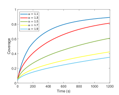
(a)

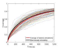
(b)

Figure 2: (a) Coverage as a function of time for $N=20$ varying $\alpha$. (b) Comparison with individual robotic simulations for $\alpha=1.3$ and $N=20$ from [18].

Fig. 2a shows the coverage as a function of time as the Lévy exponent $\alpha$ is varied for a fixed number of robots. The increasing coverage for smaller $\alpha$ confirms the advantage of long distance runs, compared with classical Brownian motion, similar to what is known for target search strategies [22, 28]. We compare these results with the average coverage of realistic individual robot simulations obtained in [18] in Figure 2b for $N=20$ and $\alpha=1.3$. These were performed with the webots simulator which recreates a real environment and includes failures. We observe a very good agreement for short and long times. The PDE description speeds up the numerical experiments by a factor $>100$ compared to the webots simulator. For a detailed comparison between the macroscopic equations from this paper and robotic simulations see [18].

The equation Eq. 67 also allows to study the dependence on the number of robots $N$. In the particular case when robots are placed sufficiently far from each other at time $t=0$, the coverage for small times will be proportional to $N$. For larger $N$ the effect of collisions becomes more important as they limit the potential long runs, but on the other hand have a volume exclusion effect.

This becomes crucial in practical situations, where all robots might be placed in a cluster in a given location at $t=0$. In this case, the coverage for small $t$ does not increase linearly with $N$, even in the absence of interactions.

9 Discussion

While macroscopic derivations based on second order models [7, 9, 27], where the velocity of the swarm changes dynamically depending on the interactions and alignment have been studied in great length, the first order models and their corresponding macroscopic PDE descriptions have received less attention.

In this paper we find macroscopic nonlocal PDE descriptions for systems arising in swarm robotics [25]. Similar to biological systems of cells or bacteria, on the microscopic scale independent agents follow a velocity jump process, for robots with collision and alignment interactions between neighbors and long range dispersal. Macroscopic swarming behaviour emerges on a hyperbolic time scale. We indicate the relevance to typical problems in swarm robotics, like target search, tracking or surveillance. Conversely, the available control in robotic systems and possibility of accurate measurements provide new modeling opportunities from microscopic to macroscopic scales.

Refined local control laws, which give rise to a desired distribution of robots, are a main topic of current research in particle swarm optimization. Biologically motivated strategies include the directed movement driven by a chemical cue, chemotaxis, which is used to devise efficient search strategies for Lévy robotic systems with sensing capabilities [45]. In bacterial foraging algorithms the length of the run or the tumbling may depend on external cues, such as pheromones, similarly leading to chemotactic behavior [53]. Also more general classes of biased random walks are of interest [14], as are control strategies obtained from machine learning. In an ongoing work we implement relevant target search strategies for systems of E–Puck robots and drones, which combine Lévy walks and collision avoidance with chemotaxis. The macroscopic PDE descriptions inform the optimal parameter settings in local control laws.

Similarly for the alignment, a wide range of interactions is being explored in robotic systems, see [48] and references therein. For example, in [35] the region of interaction may depend adaptively on the current distribution, with the aim of forming several clusters of robots. Follower-leader alignment strategies were combined with swarming models in [30, 47]. In [30] a “transient” leader ship model was considered, imitating bird flocks, where agents react in correspondence with their neighbors, while hierarchical leadership was studied in [47] within a Cucker-Smale model.

In the tumbling process, the current paper neglects delays during reorientations; we consider the tumbling phase to be much shorter than the run phase. For the system of iAnt Lévy robots in [25] waiting times are relevant, and the corresponding effect can be included into the analysis as previously done in [22]: long tailed waiting times lead to additional memory effects in time, and on long (parabolic) time scales are described by space-time fractional evolution equations. Short delays in the tumbling phase affect the diffusion coefficient $C_{\alpha}$ [51].

In all cases, rapid convergence from the initial to the desired final distribution of the robotic swarm is a main goal, and recent research has started to investigate metrics which quantify the convergence [2, 5]. Our work replaces the computationally expensive particle based models used in simulations by more efficient PDE descriptions and thereby allows efficient exploration and optimization of microscopic control laws. Detailed numerical experiments which include alignment and collision avoidance, as well as their validation against concrete robotics experiments with E–Puck robots and drones, are pursued in a current collaboration with computer scientists [18]. Complementary ongoing work considers Lévy movement in complex geometries, modeled by networks of convex domains [20].

Appendix A Collision term

We consider the interaction term only,

(68) $$\int_{\partial B_{\varrho}}\int_{S}\nu\cdot(\theta_{1}-\theta_{2})\tilde{\tilde{\sigma}}(\mathbf{x}_{1},\mathbf{x}_{2},t,\theta_{1},\theta_{2})d\theta_{2}d\mathbf{x}_{2}\ .$$

The normal vector $\nu$ at the time of collision is given by $\nu=(\mathbf{x}_{1}-\mathbf{x}_{2})/\varrho$ hence, $\mathbf{x}_{2}=\mathbf{x}_{1}-\nu\varrho$. Using $B_{\varrho}=\varrho S$ and changing variables $\nu\mapsto-\nu$, we obtain

(69) $$-\varrho^{n-1}\int_{S}\int_{S}\nu\cdot(\theta_{1}-\theta_{2})\tilde{\tilde{\sigma}}(\mathbf{x}_{1},\mathbf{x}_{1}+\nu\varrho,t,\theta_{1},\theta_{2})d\theta_{2}d\nu\ .$$

We split the outer integral into $S=S_{+}\cup S_{-}=\{\nu\cdot(\theta_{1}-\theta_{2})>0\}\cup\{\nu\cdot(\theta_{1}-\theta_{2})<0\}$, where the two individuals move towards, resp. away from, each other, hence

$$-\varrho^{n-1} \int_{S}\int_{S}\nu\cdot(\theta_{1}-\theta_{2})\tilde{\tilde{\sigma}}(\mathbf{x}_{1},\mathbf{x}_{1}+\nu\varrho,t,\theta_{1},\theta_{2})d\theta_{2}d\nu$$

$$=-\varrho^{n-1}\Bigl{[}\int_{S_{+}}\int_{S}\nu\cdot(\theta_{1}-\theta_{2})\tilde{\tilde{\sigma}}(\mathbf{x}_{1},\mathbf{x}_{1}+\nu\varrho,t,\theta_{1},\theta_{2})d\theta_{2}d\nu$$

$$\qquad+\int_{S_{-}}\int_{S}\nu\cdot(\theta_{1}-\theta_{2})\tilde{\tilde{\sigma}}(\mathbf{x_{1}},\mathbf{x}_{1}+\nu\varrho,t,\theta_{1},\theta_{2})d\theta_{2}d\nu\Bigr{]}\ .$$

In $S_{-}$ we use the collision transformation defined in Section 3, with new directions $\theta_{1}^{\prime},\theta_{2}^{\prime}$ after collision, and normal vector $-\nu$:

$$-\varrho^{n-1} \int_{S}\int_{S}\nu\cdot(\theta_{1}-\theta_{2})\tilde{\tilde{\sigma}}(\mathbf{x}_{1},\mathbf{x}_{1}+\nu\varrho,t,\theta_{1},\theta_{2})d\theta_{2}d\nu$$

$$=\varrho^{n-1}\int_{S_{+}}\int_{S}\nu\cdot(\theta_{1}-\theta_{2})\Bigl{[}\tilde{\tilde{\sigma}}(\mathbf{x}_{1},\mathbf{x}_{1}-\nu\varrho,t,\theta_{1}^{\prime},\theta_{2}^{\prime})$$

$$\qquad-\tilde{\tilde{\sigma}}(\mathbf{x}_{1},\mathbf{x}_{1}+\nu\varrho,t,\theta_{1},\theta_{2})\Bigr{]}d\theta_{2}d\nu\ .$$

Appendix B Study of alignment conditions

In this appendix we consider a specific form of the interaction kernel $K^{\varepsilon}$ and different strengths of the alignment $\ell$. We study the effect of these changes on the final system Eq. 48-Eq. 49.

Let the influence kernel $K^{\varepsilon}\left(\frac{|\mathbf{y}-\mathbf{x}|}{\varepsilon}\right)=B^{-n}e^{-\frac{|\mathbf{y}-\mathbf{x}|}{\varepsilon B}}$, where $B$ is a constant. In the case of short range alignment, $B\ll 1$, the flux term Eq. 42 can be rewritten as

(70) $$\mathcal{J}(\mathbf{x},t) =B^{-n}\int e^{-\frac{|\mathbf{y}-\mathbf{x}|}{\varepsilon B}}w(\mathbf{y},t)d\mathbf{y}=\varepsilon^{n}\int e^{-|\mathbf{y}|}w(B\varepsilon\mathbf{y}+\mathbf{x},t)d\mathbf{y}\ .$$

Taylor expansion of $w(B\varepsilon\mathbf{y}+\mathbf{x},t)$ around $B=0$ leads to (with constants $D_{1}$, $D_{2}$)

$$\mathcal{J}(\mathbf{x},t)=D_{1}\varepsilon^{n}w(\mathbf{x},t)+D_{2}\varepsilon^{n+2}B^{2}\Delta w(\mathbf{x},t)+\mathcal{O}(\varepsilon^{n+4}B^{4})\ .$$

For the alignment vector $\Lambda^{w}$, we therefore find

(71) $$\Lambda^{w}=\frac{\mathcal{J}(\mathbf{x},t)}{|\mathcal{J}(\mathbf{x},t)|}=\frac{w}{|w|}+\varepsilon^{2}B^{2}\frac{D_{2}}{D_{1}}\frac{|w|^{2}\Delta w-w(w\cdot\Delta w)}{|w|^{3}}+\mathcal{O}(\varepsilon^{4}B^{4})\ .$$

Substituting into Eq. 49 we obtain the mean direction $w$

$$w\left(1-\ell\frac{G(u)}{|w|F(u)}+\mathcal{O}(\varepsilon^{2}B^{2})\right)=-\frac{1}{F(u)}C_{\alpha}\nabla^{\alpha-1}u\ .$$

In this way we write $w$ as an explicit function of $u$ in the system Eq. 48-Eq. 49.

On the other hand, if the alignment is weak in Eq. 49 i.e., $\ell\ll 1$ , we note

(72) $$w=-\frac{1}{F(u)}C_{\alpha}\nabla^{\alpha-1}u+\ell\frac{G(u)}{F(u)}\Lambda^{u}+\mathcal{O}(\ell^{2})\ ,$$

where $\Lambda^{u}$ is written in terms of

$$\mathcal{J}^{u}(\mathbf{x},t)=-C_{\alpha}\int K^{\varepsilon}\left(\frac{|\mathbf{y}-\mathbf{x}|}{\varepsilon}\right)\frac{\nabla^{\alpha-1}u(\mathbf{y},t)}{F(u(\mathbf{y},t))}d\mathbf{y}\ .$$

In this case, the mean direction of motion of the individuals is dominated by the long runs described by the first term in Eq. 72, the alignment condition is of lower order.

Appendix C Chapman-Enskog expansion

To formally derive the expansion Eq. 56, we start from Eq. 53 and substitute Eq. 54,

$$\varepsilon(\lambda+c_{0}\theta\cdot\nabla)\hat{p}-\varepsilon p_{0}=|S|(1-\zeta)\Phi(\Lambda\cdot\theta)\Bigl{[}\varepsilon^{-\mu}A+\varepsilon^{\mu(\alpha-2)+\alpha-1}B\lambda^{\alpha-1}\Bigr{]}T^{0}\hat{p}$$

(73) $$-(\mathds{1}-\zeta T_{1})\Bigl{[}\varepsilon^{-\mu}A+\varepsilon^{\mu(\alpha-2)+\alpha-1}B(\lambda+c_{0}\theta\cdot\nabla)^{\alpha-1}\Bigr{]}\hat{p}+\mathcal{O}(\varepsilon)\ ,$$

where we have defined $T^{0}\hat{p}=|S|^{-1}\int_{S}\hat{p}d\theta$.

To the leading order $\varepsilon^{-\mu}$, Equation Eq. 73 says

(74) $$0=|S|(1-\zeta)\Phi(\Lambda\cdot\theta)\frac{\alpha-1}{\varsigma_{0}}T^{0}\hat{p}_{0}-(\mathds{1}-\zeta T_{1})\frac{\alpha-1}{\varsigma_{0}}\hat{p}_{0}\ ,$$

or equivalently $\hat{p}_{0}=\Bigl{[}|S|(1-\zeta)\Phi(\Lambda\cdot\theta)T^{0}+\zeta T_{1}\Bigr{]}\hat{p}_{0}$. For arbitrary $\zeta\in[0,1]$ and, for simplicity, $T_{1}=T^{0}$ in Eq. 73, the leading order of the solution $\hat{p}_{0}$ is given by

(75) $$\hat{p}_{0}(\mathbf{x},t,\theta)=\Phi_{\zeta}(\theta)\hat{u}(\mathbf{x},t)\ ,$$

with $\Phi_{\zeta}(\theta)=|S|(1-\zeta)\Phi(\Lambda\cdot\theta)+\zeta$. When only alignment is considered, $\zeta=0$, this reduces to the Chapman-Enskog expansion $\hat{p}_{0}=\Phi(\Lambda\cdot\theta)\hat{u}$ obtained in [15, 29], while for run and tumble processes, $\zeta=1$, one recovers the leading term of the eigenfunction expansion $\hat{p}_{0}=T_{1}\hat{p}_{0}=|S|^{-1}(\hat{u}+n\theta\cdot\hat{w})$ [21].

The next order of the expansion $\hat{p}=\hat{p}_{0}+\varepsilon^{m}\hat{p}_{1}+\mathcal{O}(\varepsilon^{2(\mu+1)(\alpha-1)})$, with $m=(\mu+1)(\alpha-1)$, is obtained from terms of order $\varepsilon^{\mu(\alpha-2)+\alpha-1}$ in Eq. 73:

(76) $$(\mathds{1}-\Phi_{\varsigma}(\theta)T^{0})\hat{p}_{1}=\frac{1}{A}\Bigl{[}(1-\zeta)\Phi(\Lambda\cdot\theta)B\lambda^{\alpha-1}-(\mathds{1}-\zeta T^{0})B(\lambda+c_{0}\theta\cdot\nabla)^{\alpha-1}\Phi_{\varsigma}(\theta)\Bigr{]}\hat{u}\ ,$$

where $A$ and $B$ are given in Eq. 55.

References

• [1] W. Alt, Biased random walk models for chemotaxis and related diffusion approximations, Journal of Mathematical Biology, 9 (1980), pp. 147–177.
• [2] B. G. Anderson, E. Loeser, M. Gee, F. Ren, S. Biswas, O. Turanova, M. Haberland, and A. L. Bertozzi, Quantitative assessment of robotic swarm coverage, arXiv preprint arXiv:1806.02488, (2018).
• [3] N. Bellomo and J. Soler, On the mathematical theory of the dynamics of swarms viewed as complex systems, Mathematical Models and Methods in Applied Sciences, 22 (2012), p. 1140006.
• [4] M. Bostan and J. A. Carrillo, Reduced fluid models for self-propelled particles interacting through alignment, Mathematical Models and Methods in Applied Sciences, 27 (2017), pp. 1255–1299.
• [5] M. Brambilla, E. Ferrante, M. Birattari, and M. Dorigo, Swarm robotics: a review from the swarm engineering perspective, Swarm Intelligence, 7 (2013), pp. 1–41.
• [6] C. Cercignani, R. Illner, and M. Pulvirenti, The mathematical theory of dilute gases, vol. 106, Springer Science & Business Media, 2013.
• [7] Y.-l. Chuang, M. R. D’orsogna, D. Marthaler, A. L. Bertozzi, and L. S. Chayes, State transitions and the continuum limit for a 2d interacting, self-propelled particle system, Physica D: Nonlinear Phenomena, 232 (2007), pp. 33–47.
• [8] M. S. Couceiro, P. A. Vargas, R. P. Rocha, and N. M. Ferreira, Benchmark of swarm robotics distributed techniques in a search task, Robotics and Autonomous Systems, 62 (2014), pp. 200–213.
• [9] F. Cucker and S. Smale, Emergent behavior in flocks, IEEE Transactions on automatic control, 52 (2007), pp. 852–862.
• [10] M. de Jager, F. J. Weissing, P. M. Herman, B. A. Nolet, and J. van de Koppel, Lévy walks evolve through interaction between movement and environmental complexity, Science, 332 (2011), pp. 1551–1553.
• [11] P. Degond, Macroscopic limits of the Boltzmann equation: a review, in Modeling and Computational Methods for Kinetic Equations, Springer, 2004, pp. 3–57.
• [12] P. Degond, A. Frouvelle, and J.-G. Liu, Macroscopic limits and phase transition in a system of self-propelled particles, Journal of Nonlinear Science, 23 (2013), pp. 427–456.
• [13] P. Degond and S. Motsch, Continuum limit of self-driven particles with orientation interaction, Mathematical Models and Methods in Applied Sciences, 18 (2008), pp. 1193–1215.
• [14] A. Dhariwal, G. S. Sukhatme, and A. A. Requicha, Bacterium-inspired robots for environmental monitoring, in Robotics and Automation, 2004. Proceedings. ICRA’04. 2004 IEEE International Conference on, vol. 2, IEEE, 2004, pp. 1436–1443.
• [15] G. Dimarco and S. Motsch, Self-alignment driven by jump processes: Macroscopic limit and numerical investigation, Mathematical Models and Methods in Applied Sciences, 26 (2016), pp. 1385–1410.
• [16] S. Dipierro, X. Ros-Oton, and E. Valdinoci, Nonlocal problems with neumann boundary conditions, Revista Matemática Iberoamericana, 33 (2017), pp. 377–416.
• [17] NIST Digital Library of Mathematical Functions. http://dlmf.nist.gov/, Release 1.0.14 of 2016-12-21, http://dlmf.nist.gov/. F. W. J. Olver, A. B. Olde Daalhuis, D. W. Lozier, B. I. Schneider, R. F. Boisvert, C. W. Clark, B. R. Miller and B. V. Saunders, eds.
• [18] S. Duncan, G. Estrada-Rodriguez, J. Stocek, et al., Efficient quantitative assessment of robot swarms: coverage and targeting lévy strategies, preprint, (2019).
• [19] R. Erban and H. G. Othmer, From individual to collective behavior in bacterial chemotaxis, SIAM Journal on Applied Mathematics, 65 (2004), pp. 361–391.
• [20] E. Estrada, G. Estrada-Rodriguez, and H. Gimperlein, Metaplex networks: influence of the exo-endo structure of complex systems on diffusion, SIAM Review, 62 (2020), p. to appear.
• [21] G. Estrada-Rodriguez, H. Gimperlein, and K. J. Painter, Fractional Patlak–Keller–Segel equations for chemotactic superdiffusion, SIAM Journal on Applied Mathematics, 78 (2018), pp. 1155–1173.
• [22] G. Estrada-Rodriguez, H. Gimperlein, K. J. Painter, and J. Stocek, Space-time fractional diffusion in cell movement models with delay, Mathematical Models and Methods in Applied Sciences, 29 (2019), pp. 65–88.
• [23] S. Fedotov and N. Korabel, Emergence of Lévy walks in systems of interacting individuals, Physical Review E, 95 (2017), p. 030107.
• [24] B. Franz, J. P. Taylor-King, C. Yates, and R. Erban, Hard-sphere interactions in velocity-jump models, Physical Review E, 94 (2016), p. 012129.
• [25] G. M. Fricke, J. P. Hecker, J. L. Cannon, and M. E. Moses, Immune-inspired search strategies for robot swarms, Robotica, 34 (2016), pp. 1791–1810.
• [26] H. Gimperlein and J. Stocek, Space–time adaptive finite elements for nonlocal parabolic variational inequalities, Computer Methods in Applied Mechanics and Engineering, 352 (2019), pp. 137–171.
• [27] S.-Y. Ha and E. Tadmor, From particle to kinetic and hydrodynamic descriptions of flocking, Kinetic & Related Models, 1 (2008), pp. 415–435.
• [28] T. Harris et al., Generalized Lévy walks and the role of chemokines in migration of effector CD8+ T cells, Nature, 486 (2012), pp. 545–548.
• [29] B. Jacek et al., Singularly perturbed evolution equations with applications to kinetic theory, vol. 34, World Scientific, 1995.
• [30] A. Jadbabaie, J. Lin, and A. S. Morse, Coordination of groups of mobile autonomous agents using nearest neighbor rules, IEEE Transactions on Automatic Control, 48 (2003), pp. 988–1001.
• [31] G. Kantor, S. Singh, R. Peterson, D. Rus, A. Das, V. Kumar, G. Pereira, and J. Spletzer, Distributed search and rescue with robot and sensor teams, in Field and Service Robotics, Springer, 2003, pp. 529–538.
• [32] E. H. Kennard et al., Kinetic theory of gases, with an introduction to statistical mechanics, McGraw-Hill, 1938., 1938.
• [33] E. Korobkova, T. Emonet, J. M. Vilar, T. S. Shimizu, and P. Cluzel, From molecular noise to behavioural variability in a single bacterium, Nature, 428 (2004), pp. 574–578.
• [34] M. Krivonosov, S. Denisov, and V. Zaburdaev, Lévy robotics, arXiv preprint arXiv:1612.03997, (2016).
• [35] X. Li, Adaptively choosing neighbourhood bests using species in a particle swarm optimizer for multimodal function optimization, in Genetic and Evolutionary Computation Conference, Springer, 2004, pp. 105–116.
• [36] F. Mondada and et al., The e-puck, a robot designed for education in engineering, in Proceedings of the 9th Conference on Autonomous Robot Systems and Competitions, 2009, pp. 59–65.
• [37] S. Motsch and E. Tadmor, A new model for self-organized dynamics and its flocking behavior, Journal of Statistical Physics, 144 (2011), p. 923.
• [38] S. G. Nurzaman, Y. Matsumoto, Y. Nakamura, S. Koizumi, and H. Ishiguro, Yuragi-based adaptive searching behavior in mobile robot: From bacterial chemotaxis to Lévy walk, in Robotics and Biomimetics, 2008. ROBIO 2008. IEEE International Conference on, IEEE, 2009, pp. 806–811.
• [39] H. G. Othmer and T. Hillen, The diffusion limit of transport equations derived from velocity-jump processes, SIAM Journal on Applied Mathematics, 61 (2000), pp. 751–775.
• [40] H. G. Othmer and T. Hillen, The diffusion limit of transport equations ii: Chemotaxis equations, SIAM Journal on Applied Mathematics, 62 (2002), pp. 1222–1250.
• [41] Z. Pasternak, F. Bartumeus, and F. W. Grasso, Lévy-taxis: a novel search strategy for finding odor plumes in turbulent flow-dominated environments, Journal of Physics A: Mathematical and Theoretical, 42 (2009), p. 434010.
• [42] C. S. Patlak, Random walk with persistence and external bias, The Bulletin of Mathematical Biophysics, 15 (1953), pp. 311–338.
• [43] B. Perthame, W. Sun, and M. Tang, The fractional diffusion limit of a kinetic model with biochemical pathway, Zeitschrift für angewandte Mathematik und Physik, 69 (2018), p. 67.
• [44] G. Ramos-Fernández, J. L. Mateos, O. Miramontes, G. Cocho, H. Larralde, and B. Ayala-Orozco, Lévy walk patterns in the foraging movements of spider monkeys (Ateles geoffroyi), Behavioral Ecology and Sociobiology, 55 (2004), pp. 223–230.
• [45] A. Schroeder, S. Ramakrishnan, M. Kumar, and B. Trease, Efficient spatial coverage by a robot swarm based on an ant foraging model and the Lévy distribution, Swarm Intelligence, 11 (2017), pp. 39–69.
• [46] M. Senanayake, I. Senthooran, J. C. Barca, H. Chung, J. Kamruzzaman, and M. Murshed, Search and tracking algorithms for swarms of robots: A survey, Robotics and Autonomous Systems, 75 (2016), pp. 422–434.
• [47] J. Shen, Cucker–Smale flocking under hierarchical leadership, SIAM Journal on Applied Mathematics, 68 (2007), pp. 694–719.
• [48] R. Shvydkoy and E. Tadmor, Topological models for emergent dynamics with short-range interactions, arXiv preprint arXiv:1806.01371, (2018).
• [49] D. K. Sutantyo, S. Kernbach, P. Levi, and V. A. Nepomnyashchikh, Multi-robot searching algorithm using Lévy flight and artificial potential field, in Safety Security and Rescue Robotics (SSRR), 2010 IEEE International Workshop on, IEEE, 2010, pp. 1–6.
• [50] Y. Tan and Z.-y. Zheng, Research advance in swarm robotics, Defence Technology, 9 (2013), pp. 18–39.
• [51] J. P. Taylor-King, B. Franz, C. A. Yates, and R. Erban, Mathematical modelling of turning delays in swarm robotics, IMA Journal of Applied Mathematics, 80 (2015), pp. 1454–1474.
• [52] J. P. Taylor-King, R. Klages, S. Fedotov, and R. A. Van Gorder, Fractional diffusion equation for an n-dimensional correlated Lévy walk, Physical Review E, 94 (2016), p. 012104.
• [53] M. Turduev, M. Kirtay, P. Sousa, V. Gazi, and L. Marques, Chemical concentration map building through bacterial foraging optimization based search algorithm by mobile robots, in Systems Man and Cybernetics (SMC), 2010 IEEE International Conference on, IEEE, 2010, pp. 3242–3249.
• [54] G. Varela, P. Caamaño, F. Orjales, Á. Deibe, F. Lopez-Pena, and R. J. Duro, Swarm intelligence based approach for real time uav team coordination in search operations, in Nature and Biologically Inspired Computing (NaBIC), 2011 Third World Congress on, IEEE, 2011, pp. 365–370.
• [55] T. Vicsek, A. Czirók, E. Ben-Jacob, I. Cohen, and O. Shochet, Novel type of phase transition in a system of self-driven particles, Physical review letters, 75 (1995), p. 1226.
• [56] C. Xue, H. G. Othmer, and R. Erban, From individual to collective behavior of unicellular organisms: recent results and open problems, in AIP Conference Proceedings, vol. 1167, AIP, 2009, pp. 3–14.
• [57] F. Zhang, A. L. Bertozzi, K. Elamvazhuthi, and S. Berman, Performance bounds on spatial coverage tasks by stochastic robotic swarms, IEEE Transactions on Automatic Control, 63 (2018), pp. 1563–1578.