Pseudo-scalar $q\bar{q}$ bound states at finite temperatures within a Dyson-Schwinger–Bethe-Salpeter approach

Abstract

The combined Dyson-Schwinger–Bethe-Salpeter equations are employed at non-zero temperature. The truncations refer to a rainbow-ladder approximation augmented with an interaction kernel which facilitates a special temperature dependence. At low temperatures, $T\to 0$, we recover a quark propagator from the Dyson-Schwinger (gap) equation which delivers, e.g. mass functions $B$, quark renormalization wave function $A$, and two-quark condensate $\langle q\bar{q}\rangle$ smoothly interpolating to the $T=0$ results, despite the broken O(4) symmetry in the heat bath and discrete Matsubara frequencies. Besides the Matsubara frequency difference entering the interaction kernel, often a Debye screening mass term is introduced when extending the $T=0$ kernel to non-zero temperatures. At larger temperatures, however, we are forced to drop this Debye mass in the infra-red part of the longitudinal interaction kernel to keep the melting of the two-quark condensate in a range consistent with lattice QCD results. Utilizing that quark propagator for the first few hundred fermion Matsubara frequencies we evaluate the Bethe-Salpeter vertex function in the pseudo-scalar $q\bar{q}$ channel for the lowest boson Matsubara frequencies and find a competition of $q\bar{q}$ bound states and quasi-free two-quark states at $T={\cal O}$ (100 MeV). This indication of pseudo-scalar meson dissociation below the anticipated QCD deconfinement temperature calls for an improvement of the approach, which is based on an interaction adjusted to the meson spectrum at $T=0$.

I Introduction

The description of mesons as quark-antiquark bound states within the framework of the Bethe-Salpeter (BS) equation with momentum dependent quark mass functions, determined by the Dyson-Schwinger (DS equation, is able to explain successfully many spectroscopic data, such as meson masses fishJPA ; Thomas ; rob-1 ; MT ; ourLast ; Hilger ; Maris:2003vk ; Holl:2004fr ; Blank:2011ha , electromagnetic properties of pseudoscalar mesons and their radial excitations Jarecke:2002xd ; Krassnigg:2004if ; Roberts:2007jh and other observables ourFB ; wilson ; JM-1 ; JM-2 ; rob-2 ; Alkofer ; fisher ; Roberts:2007jh . Contrary to purely phenomenological models, like the quark bag model, such a formalism maintains important features of QCD, such as dynamical chiral symmetry breaking, dynamical quark dressing, requirements of the renormalization group theory etc., cf. Ref. physRep . The main ingredients here are the full quark-gluon vertex function and the dressed gluon propagator, which are entirely determined by the running coupling and the bare quark mass parameters. In principle, if one were able to solve the Dyson-Schwinger equations for the quark propagator, the gluon propagator, the quark-gluon and inter-gluon vertices , supplemented by ghosts if necessary, then the approach would not depend on any additional parameters. In practice, one restricts oneself to calculations within effective models which specify the dressed vertex function $\Gamma_{\mu}$ (for quark-gluon coupling) and interaction kernel $D_{\mu\nu}$ (for the gluon propagator). The rainbow-ladder approximation MT is a model with rainbow truncation of the vertex function $\Gamma_{\mu}\to\gamma_{\mu}$ in the quark DS equation and a specification of the dressed quark-quark interaction kernel (for gluon exchanges) as $g^{2}D_{\mu\nu}(k)\to{\cal G}(k^{2})D_{\mu\nu}^{free}(k)$ within the Landau gauge. (Here, $\gamma_{\mu}$ is a Dirac gamma matrix and $D_{\mu\nu}$ stands for the gluon propagator; $g$ is the coupling strength and $k$ denotes a momentum.)

The model is completely specified once a form is chosen for the “effective coupling” ${\cal G}(k^{2})$. The ultraviolet behavior is chosen to be that of the QCD running coupling $\alpha_{s}(k^{2})=g^{2}(k^{2})/4\pi$ computed within one-loop approximation; the ladder-rainbow truncation then generates the correct perturbative QCD structure of the DS and BS equations. Moreover, the ladder-rainbow truncation preserves such an important feature of the theory as the maintenance of the Nambu-Goldstone theorem in the chiral limit, according to which the spontaneous chiral symmetry breaking results in an appearance of a (otherwise absent) scalar term in the quark propagator of the DS equation. As a consequence, in the BS equation a massless pseudoscalar bound state should appear. By using the Ward identities, it has been proven (see, e.g. Refs. smekal ; scadron ; munczek ) that, in the chiral limit, the DS equation for the quark propagator and the BS equation for a massless pseudo-scalar in ladder approximation are completely equivalent. It implies that such a massless bound state (pion) can be interpreted as a Goldstone boson. This results in a straightforward understanding of the pion as a Goldstone boson and quark-antiquark bound state at the same time.

Another important property of the DS and BS equations is that, at zero temperatures, or equivalently - in vacuum - they are explicitly Poincaré invariant. This frame-independency of the approach provides a useful tool in studying processes where a rest frame for mesons cannot or needs not be defined. A rather different situation is encountered at finite temperatures, where a particle is embedded in a heat bath. In this case, the propagator of the particle is defined by two four-vectors, the four-momentum $p$ of the particle and a unit four-vector $u$ characterizing the heat bath itself hatsuda ; Ayale ; RobProg . The scalar parts of the propagator then depend on $p^{2}$ and $(up)$. An existence of the statistical thermal factor $\exp(-H/T)$, $H$ being the QCD hamiltonian, implies the choice of the unit vector $u$ as $u=({\bf 0},1)$, i.e. the heat bath at rest hatsuda . As a consequence, the O(4) symmetry of equations is lost and only the spatial translation invariance is maintained. This requires a separate treatment of the transversal and longitudinal, with respect to the heat bath, parts of the kernel with the need of additional functions in parametrizing the quark propagators and the BS vertex functions.

In quantum field theory, a system at finite temperature can be described within the imaginary-time formalism, which uses the Matsubara frequancies matzubara ; kapusta ; abrikosov . Due to finiteness of the heat bath temperature $T$ and the requirements of periodicity (bosons) or antiperiodicity (fermions) of the considered fields periodic ; KMS ; kapusta ; abrikosov , the Fourier transform to Euclidean momentum space becomes discrete in the time direction, resulting in a discrete spectrum of the energy, known as the Matsubara frequencies. Consequently, the interaction kernel and the DS and BS solutions must become also discrete with respect to these frequencies. It is worth mentioning that there is no straight forward connection of the obtained solutions in the discrete Euclidean space to the corresponding continuum quantities in Minkowski space fisher1 ; roberts ; yaponetz . In particular, within the Matsubara formalism one can define the mass of the bound state in different ways in dependence of the choice of the total momentum $P=({\bf P},i\Omega_{N})$; at $N=0$ one defines the so-called screening mass, which has no direct relation with the usual inertial mass. At $|{\bf P}|\neq 0$ and $N\neq 0$ the corresponding pole mass $P^{2}=-M^{2}$ is also discrete and hitherto it is note clearly established how to relate it to the inertial mass. In principle, at each particular choice of $P$ one can define a quark correlator and try to define the inertial mass by computing the momentum Fourier transforms and the resulting spatial integral of the correlator (analogue of the 2-points Schwinger functions, see e.g. robertsSchwinger ) and by taking the time derivative of the logarithm of the obtained expression, see also fisher1 ; roberts ; yaponetz ; physrepMorley ; blaske . Evidently, such a procedure requires knowledge of the pole mass for all, or at least for a large enough number of Matsubara frequencies. It is worth mentioning that a growing interest nowadays is in approaches based on real-time calculations of quark and gluon propagators and their spectral functions within the functional renormalization group frg1 ; frg2 ; frg3 . These approaches also require analytical continuation of the propagators from Euclidean to Minkowski spaces.

In the present paper, we calculate the pole masses of pseudo-scalar quark-antiquark bound-states only for the few first Matsubara frequencies and investigate their dependence on temperature in a large interval, including the ”dissociation region”. We anticipate that the main peculiarities of masses computed at some particular Matsubara frequencies will reflect the general $T$ dependence of the inertial masses at high temperatures. We treat the bound states within the BS formalism within the same approach as the one used in solving the DS equation, i.e. with the rainbow truncation and AWW interaction kernel Alkofer . Recall that the merit of the approach is that, once the effective parameters are fixed (usually the effective parameters of the kernel are chosen, cf. Refs. Parameterslattice ; williams , to reproduce the known ”experimental” data from lattice calculations, such as the quark mass function and/or quark condensate, the whole spectrum of known mesons is supposed to be described, on the same footing, including also excited states. The achieved amazingly good description of the mass spectrum with only few effective parameters encourages one to employ the same approximations to the DS and BS equations also at finite temperatures with the hope that, once an adequate description of the quark propagators at non-zero temperature is accomplished, the corresponding solution can be implemented into the BS equation for mesons to investigate the meson properties in hot matter.

At low temperatures, the properties of hadrons in nuclear matter are expected to change in comparison with the vacuum ones, however, the main quantum numbers, such as spin and orbital momenta, space and inner parities etc. are maintained. The hot environment may modify the hadron masses, life times (decay constants) etc. Contrarily, at sufficiently large temperature in hot and dense strongly interacting matter, (phase) transitions may occur, related to quark deconfinement phenomena, as e.g. dissociation of hadrons into quark-gluon degrees of freedom. Therefore, this temperature region is of great interest, both from a theoretical and experimental point of view. So far, the truncated DS and BS formalism has been mostly used at large temperatures to investigate the critical phenomena near and above the pseudo-critical and (phase) transition values predicted by lattice simulation data (cf. Refs. kitaizyRpberts ; MTrenorm ; rischke ; ourModernPhys ). It has been found that, in order to achieve an agreement of the model results with lattice data, a modification of the vacuum interaction kernel is required. First of all it has been observed that modifications of the (pure phenomenological, nonperturbative) infra-red (IR) term by including the $T$ dependence of the perturbative Debye mass results in an essential suppression of the longitudinal interaction kernel at large temperatures BlankKrass ; ourModernPhys . As a consequence, the predicted critical temperatures $T_{c}$ of chiral symmetry restoration in the chiral limit and also the critical temperatures for the maximum of chiral susceptibility, as well as of inflection point of the mass function or of the quark condensate, are much smaller, by about 50%, than that expected from the lattice calculations. It became evident that modifications of the IR term at large temperatures are necessary. Namely, the IR term has to vanish abruptly in this region and to be replaced by another phenomenological kernel. For instance, it has been suggested kitaizyRpberts ; robLast to employ a kernel with a Heavyside step-like behaviour in the vicinity of the (pseudo-) critical temperature $T_{c}$. Then, it becomes possible to achieve a rather reliable description of such quantities as the quark spectral function, plasmino modes, thermal masses etc., see also Ref. kitazavaPRD80 . However, a use of such a discontinuously modified interaction in the BS equation in the whole temperature range becomes hindered.

Another strategy of solving the DS equation in a larger interval of temperatures is to utilize directly the available results of nonperturbative lattice QCD (LQCD) calculations to fit, point by point, the interaction kernel at given temperatures. In such a way one achieves a good description of the quark mass function and condensate for different temperatures, including the region beyond $T_{c}$ fischerPRD90 ; FischerRenorm . The success of such approaches demonstrates that the rainbow approximation to the DS equation with a proper choice of the interaction kernel is quite adequate in understanding the properties of quarks in a hot environment. Nevertheless, for systematic studies of quarks and hadrons within the BS equation, on needs a smooth parametrization of the kernel in the whole interval of the considered temperatures. In view of still scarce LQCD data, such a direct parametrization from ”experimental” data is problematic. An alternative method is to solve simultaneously a (truncated) set of Dyson-Schwinger equations for the quark and gluon propagators within some additional approximations fischerGluon . This approach also provides good description of the quark mass function and condensate in vicinity of $T_{c}$, however it becomes too cumbersome in attempts to solve the BS equation, since in this case one should solve a too large system of equations. It should also be noted that there are other investigations of the quark propagator within the rainbow truncated DS equation, which employ solely the vacuum parameters in calculations of $T$ dependencies of quarks BlankKrass without further attempts to accommodate to LQCD results in the kernel. As a result one finds that the critical behaviour of the propagators (e.g. chiral symmetry restoration) starts at temperatures much smaller than the ones expected from LQCD.

In the present paper we are interested in a qualitative study of the masses of quark-antiquark bound states at moderate and large temperatures. Particular attention is paid to the region where the bound state mass becomes larger than the sum of two masses of free quarks. This temperature range probably indicates a dissociation of the ground bound state and existence of only highly excited correlations. For such a qualitative analysis we employ the simplest version of the kernel which consists of only the infra-red term of the Maris-Tandy MT kernel, known also as the Alkofer-Watson-Weigel Alkofer kernel, referred to as the AWW model. For further kernels cf. MT ; robLast ; BlankKrass ; otherKernels1 ; otherKernels2 ; otherKernels3 , in particular to symmetry preserving issues and going beyond the rainbow-ladder approximation. As mentioned above, including of the Debye mass in this term results in too low values of the critical temperatures, and a proper modification is needed. For this sake, in the present paper we ignore the Debye mass which allows to obtain solutions of the DS equation with characteristics close to that of lattice calculations. However, for completeness we also present some results of calculations with accounting of the Debye mass too. We start with the AWW interaction kernel, known at $T=0$ to provide a good description of the mass spectrum of scalar, pseudo-scalar, vector and tensor mesons. Then we extend the DS and BS equations to finite temperatures and solve the corresponding equations in a large interval of $T$ and Matsubara frequencies. Results of calculations are compared with masses of free quarks.

Our paper is organized as follows. In Sec. II, we recall the truncated Dyson-Schwinger (tDS) and truncated Bethe-Salpeter (tBS) equations in vacuum and at finite temperatures. The rainbow approximation for the DS equation kernel in vacuum is introduced and the system of equations for the quark propagator is solved.

Numerical solutions for the quark propagator at finite bare quark masses are discussed in Sec. III, where the inflection points of the quark condensate and the mass function are considered as a definition of the pseudo-critical temperature $T_{c}$. It is shown that, for finite quark masses, the inflection method determines the pseudo critical temperatures by $\sim 50\%$ smaller than the ones obtained by other approaches, e.g. by LQCD calculations. It is found that, by merely ignoring the Debye mass in the infra-red term, it becomes possible to reconcile the model and lattice QCD results; the such obtained values of $T_{c}\sim 135$ MeV is only by about $10-15$% smaller then the lattice results (reported, e.g. in Refs. yoki ; FischerRenorm ). In Sec. IV we generalize the tBS equation to finite temperature by exploring the same procedure as that used in generalizing the tDS equation to finite $T$. As already mentioned, due to the breaking of the O(4) symmetry, the tBS equation cannot be longer considered for mesons at rest. The total momentum $P^{2}=-M^{2}_{qq}$ is replaced as $P({\bf 0},iM_{qq})\rightarrow P({\bf P},iE)$, where now the energy $E$ becomes discrete and depends on the Matsubara frequency $\Omega_{N}=2\pi NT$. In dependence of the chosen components of the total momentum $P$, one can define at least three different ground state masses: (i) the thermal mass at ${\bf P}=0$, $M^{2}=(2\pi N)^{2}T^{2}$, (ii) the imaginary screening mass at zero Matsubara frequency $n=0$, ${\bf P}^{2}=-M^{2}$ and (iii) the pole mass $M^{2}=(2\pi N)^{2}T^{2}-{\bf P}^{2}$. In principle, these masses are not obligatorily the same at given temperature $T$, as discussed in Refs. fisher1 ; yaponetz ; blaske ; roberts , for instance. In the present paper, we consider the pole masses which at given temperature and Matsubara frequency are continuous functions of the three momentum ${\bf P}^{2}$.

Summary and conclusions are collected in Sec. VII.

II Basic Formulae

II.1 Truncated Dyson-Schwinger and Bethe-Salpeter equations in vacuum

To determine the bound-state mass of a quark-antiquark pair one needs to solve the DS and the homogeneous BS equations, which in the rainbow ladder approximation and in Euclidean space read

$$S^{-1}(p)=S_{0}^{-1}(p)+\frac{4}{3}\int\frac{d^{4}k}{(2\pi)^{4}}\left[g^{2}{D}_{\mu\nu}(p-k)\right]\gamma_{\mu}S(k)\gamma_{\nu}\>,$$ (1)

$$\Gamma(P,p)=-\frac{4}{3}\int\frac{d^{4}k}{(2\pi)^{4}}\gamma_{\mu}S(\eta_{1}P+k)\Gamma(P,k)S(-\eta_{2}P+k))\gamma_{\nu}\left[g^{2}{D}_{\mu\nu}(p-k)\right]\>,$$ (2)

where $\eta_{1}$ and $\eta_{2}=1-\eta_{1}$ are the partitioning parameters defining the quark momenta as $p_{1,2}=k\pm\eta_{1,2}P$ with $P$, $p$ and $k$ denoting the total and relative momenta of the bound system, respectively; $\Gamma(P,k)$ stands for the tBS vertex function being a $4\times 4$ matrix, $S_{0}(p)=\left(i\gamma\cdot p+m\right)^{-1}$ and $S(p)=\left(i\gamma\cdot pA(p)+B(p)\right)^{-1}$ are the propagators of bare and dressed quarks, respectively, with mass parameter $m$ and the dressing functions $A(p)$ and $B(p)$. At zero temperature the above equations are O(4) invariant and the propagator functions $A(p)$ and $B(p)$ depend solely on $p^{2}={\bf p}^{2}+p_{4}^{2}$. The total momentum $P=({\bf 0},iM_{q\bar{q}})$, for a particle at rest, is an external parameter for (2); the momenta of individual quarks are $p_{1,2}^{2}=-M^{2}_{q\bar{q}}/4+k^{2}\pm iM_{qq}k_{4}$, where the Euclidean components $\bf k$ and $k_{4}$ of the relative momentum are defined as $k^{2}={\bf k}^{2}+k_{4}^{2}$ which, for the BS equation, are the integration variables. In order to reduce the four-dimensional integral to a two-dimensional one, usually the phase space volume is parametrized by the Euclidean modulus $k$, a hyperangle $\chi_{k}$ defined as $|{\bf k}|=k\sin\chi_{k},\ k_{4}=k\cos\chi_{k}$ and by the standard angular space volume $d\Omega_{\bf k}$. Then the tBS vertex functions $\Gamma(P,k)$ are decomposed over the hyperspherical harmonics basis which allow to carry out the spacial angular integration analytically (see for details Refs. ourLast ; ourFB ; DorkinByer ). The resulting tBS equation represents a system of two-dimensional integral equations, where the vectors $p_{1,2}$ vary in a restricted complex domain located within parabolas $p_{1,2}^{2}=-M^{2}_{q\bar{q}}/4+k^{2}\pm iM_{q\bar{q}}k\cos\chi_{k}$. In Euclidean space the Dirac matrices $\gamma_{4}=\gamma_{0},{\mbox{\boldmath$\gamma$}}_{E}=-i{\mbox{\boldmath$\gamma$}}_{M}$ are Hermitian and obey the anti-commutation relation $\{\gamma_{\mu},\gamma_{\nu}\}=2\delta_{\mu,\nu}$; for the four-product one has $(a\cdot b)={\bf ab}+a_{4}b_{4}$ . The masses $M_{q\bar{q}}$ of mesons as bound states of a $m_{1}$-quark and $m_{2}$-antiquark follow from the solution of the tBS equation at $P^{2}=-M_{q\bar{q}}^{2}$ in specific $J^{PC}$ channels, with the solution of the tDS equation (1) as input into the calculations in Eq. (2). The interaction between quarks in the pair is encoded in $g^{2}D_{\mu\nu}$, imagined as gluon exchange. For consistency, the same interaction is to be employed in the tDS equation (1) for the inverse dressed quark propagator.

Often, the coupled equations of the quark propagator $S$, the gluon propagator $D_{\mu\nu}$ and the quark-gluon vertex function $\Gamma_{\mu}$ (not to be confused with the BS vertex function $\Gamma(P,p)$), all with full dressing (and, if needed, supplemented by ghosts and their respective vertices), are considered as an integral formulation being equivalent to QCD. In practice, due to numerical problems, the finding of the exact solution of the system of coupled equations for $S-D_{\mu\nu}-\Gamma_{\mu}$ can hardly be accomplished and therefore some approximations fisher ; Maris:2003vk ; physRep are appropriate. Being interested in dealing with mesons as quark-antiquark bound states of the BS equation (2), one has to provide the quark propagator which depends on the gluon propagator and vertex as well, which in turn depend on the quark propagator. Leaving a detailed discussion of the variety of approaches in dressing of the gluon propagator and vertex function in DS equations (see e.g. Refs. Fischer:2008uz ; PenningtonUV and references therein quoted) we mention only that in solving the DS equation for the quark propagator one usually employs truncations of the exact interactions and replaces the gluon propagator combined with the vertex function by an effective interaction kernel $[g^{2}D_{\mu\nu}]$. This leads to the tDS equation for the quark propagator which may be referred to as the gap equation. In explorative calculations, the choice of the form of the effective interaction is inspired by results from calculations of Feynman diagrams within pQCD maintaining requirements of symmetry and asymptotic behaviour already implemented, cf. Refs. Maris:2003vk ; Roberts:2007jh ; physRep ; PenningtonUV . The results of such calculations, even in the simple case of accounting only for one-loop diagrams with proper regularization and renormalization procedures, are rather cumbersome for further use in numerical calculations, e.g. in the framework of BS or Faddeev equations. Consequently, for practical purposes, the wanted exact results are replaced by suitable parametrizations of the vertex and the gluon propagator. Often, one employs an approximation which corresponds to one-loop calculations of diagrams with the full vertex function $\Gamma_{\nu}$, substituted by the free one, $\Gamma_{\nu}(p,k)\rightarrow\gamma_{\nu}$ (we suppress the color structure and account cumulatively for the strong coupling later on). To emphasize the replacement of combined gluon propagator and vertex (in the Landau gauge) we use the notation $[g^{2}D_{\mu\nu}]$, where an additional power of $g$ from the second undressed vertex is included.

II.2 Choosing an interaction kernel

Note that the nonperturbative behaviour of the kernel $[g^{2}D_{\mu\nu}]$ at small momenta, i.e. in the infra-red (IR) region, nowadays is not uniquely determined and, consequently, suitable models are needed. There are several ansätze in the literature for the IR kernel, which can be formally classified in the two groups: (i) the IR part is parametrized by two terms - a delta distribution at zero momenta and an exponential, i.e. Gaussian term, and (ii) only the Gaussian term is considered. In principle, the IR term must be supplemented by a ultraviolet (UV) one, which assures the correct asymptotics at large momenta. A detailed investigation souglasInfrared ; Blank:2011ha of the interplay of these two terms has shown that, for bound states, the IR part is dominant for light ($u$, $d$ and $s$) quarks with a decreasing role for heavier ($c$ and $b$) quark masses for which the UV part may be quite important in forming mesons with masses $M_{q\bar{q}}>3-4$ GeV as bound states. In the vacuum, if one is interested in an analysis of light mesons with $M_{q\bar{q}}\leq 3-4$ GeV, the UV term can be omitted.

Following examples in the literature Alkofer ; MT ; Maris:2003vk ; Krassnigg:2004if ; wilson ; Roberts:2007jh the interaction kernel in the rainbow approximation in the Landau gauge is chosen as

$$g^{2}(k^{2}){\cal D}_{\mu\nu}(k^{2})=\left(D_{IR}(k^{2})+D_{UV}(k^{2})\right)\left(\delta_{\mu\nu}-\frac{k_{\mu}k_{\nu}}{k^{2}}\right),$$

$$D_{IR}(k^{2})=\frac{4\pi^{2}Dk^{2}}{\omega^{6}}e^{-k^{2}/\omega^{2}},\ \quad D_{UV}(k^{2})=\frac{8\pi^{2}\gamma_{m}F(k^{2})}{\ln\left[\tau+\left(1+\frac{k^{2}}{\Lambda_{QCD}^{2}}\right)^{2}\right]},$$ (3)

where the first term originates from the effective IR part of the interaction determined by soft, non-perturbative effects, while the second one ensures the correct UV asymptotic behaviour of the QCD running coupling, $F(k^{2})=\{1-\exp(-k^{2}/[4m_{t}^{2}])\}/k^{2}$ with $m_{t}$ as an adjustable parameter, $m_{t}\simeq 0.5$ GeV, and $\tau=e^{2}-1$, $\Lambda_{QCD}=0.234$ GeV, and $\gamma_{m}=12/(33-2N_{f})$ for $N_{f}$ as active flavors. In what follows we restrict ourselves to the simplest version of the model, namely with the interaction kernel where the UV term (the effect of which is found souglasInfrared to be negligibly small) is ignored at all. As said above, this interaction is the Alkofer-Watson-Weigel Alkofer kernel. A prominent feature of such an interaction is that, with only a few adjustable parameters - $D$, $\omega$ in the IR term and quark mass parameter $m$ in the bare quark propagator $S_{0}$ - it provides a good description of the pseudoscalar, vector and tensor meson mass spectra Hilger ; Holl:2004fr ; Blank:2011ha ; ourLast at zero temperature. It should be noted that, despite the negligible contribution, the inclusion of the UV term in the numerical calculations causes additional uncertainties, related to the divergency of the integrals and with requirements of regularization and subtraction procedures FischerRenorm . Therefore, at finite temperatures a tempting choice of the interaction is to keep the AWW kernel the same as in vacuum. Notice also that, even at zero temperatures, the tBS equation becomes rather complicate for numerical solutions since it involves the quark propagator functions in the complex Euclidean space, where they can (actually they do) exhibit pole-like singularities. A rather detailed analysis of solving the tBS equation in vacuum in presence of poles has been reported in Ref. ourLast . Reiterate that, within the rainbow approximation, the Euclidean $P_{4}=iM_{q\bar{q}}$ is an external parameter in the tBS equation, while $k_{4}$ is an integration variable.

II.3 Finite temperatures

The theoretical treatment of systems at non-zero temperatures differs from the case of zero temperatures. In this case, a preferred frame is determined by the local rest system of the thermal bath. This means that the $O(4)$ symmetry is broken and, consequently, the dependence of the quark propagator on $\bf p$ and $p_{4}$ requires a separate treatment. To describe the propagator in this case a third function $C$ is needed, besides the functions $A$ and $B$ introduced above for vacuum. Yet, the theoretical formulation of the field theory at finite temperatures can be performed in at least two, quite different, frameworks which treat fields either with ordinary time variable $t\,(-\infty<t<\infty)$, e.g. the termo-field dynamics (cf. umezawa ) and path-integral formalism (cf. nemi ; landshof ), or with imaginary time $it=\tau$ ($0<\tau<1/T$) which is known as the Matsubara formalism matzubara ; kapusta ; abrikosov ; landsman . In this paper we utilize the imaginary-time formalism within which the partition function is defined and all calculations are performed in Euclidean space. Since, due to the Kubo–-Martin-–Schwinger condition periodic ; KMS ; Sch ; kapusta for equilibrium systems, the (imaginary) time evolution is restricted to the interval $[0\ldots 1/T]$, the quark fields become anti-periodic in time with the period $1/T$. In such a case, the Fourier transform is not longer continuous and the energies $p_{4}$ of particles become discrete matzubara ; kapusta ; abrikosov which are known as the Matsubara frequencies, i.e. $p_{4}=\omega_{n}=\pi T(2n+1)$ for Fermions ($n\in\mathbb{Z}$). The inverse quark propagator is now parametrized as

$$S^{-1}({\bf p},\omega_{n})=i{\mbox{\boldmath$\gamma$}}{\bf p}A({\bf p}^{2},\omega_{n}^{2})+i\gamma_{4}p_{4}C({\bf p}^{2},\omega_{n}^{2})+B({\bf p}^{2},\omega_{n}^{2}).$$ (4)

Accordingly, the interaction kernel is decomposed in to a transversal and longitudinal part

$$[g^{2}D_{\mu\nu}({\bf k},\Omega_{mn})]={\cal P}^{T}_{\mu\nu}D^{T}({\bf k},\Omega_{mn},0)+{\cal P}^{L}_{\mu\nu}D^{L}({\bf k},\Omega_{mn},m_{g}),$$ (5)

where $\Omega_{mn}=\omega_{m}-\omega_{n}$ and the gluon Debye screening mass $m_{g}$ is introduced in the longitudinal part of the propagator, where $k^{2}={\bf k}^{2}+\Omega_{mn}^{2}+m_{g}^{2}$ enters. The Debye mass describes perturbatively the screening of chromoelectric fields at large temperatures, therefore it is relevant for the perturbative UV term in the limit of quark-gluon plasma where the light-quark bound states do not longer exists, and the system ie to be described by quark and gluon degrees of greedom. As for the nonperturbative pure phenomenological IR term, it is not a priory clear whether the Debye mass has to be implemented in the IR term or not. We consider both possibilities, with and without the Debye mass in the AWW model.

The scalar coefficients $D^{L,T}$ are defined below. The projection operators ${\cal P}_{\mu\nu}^{L,T}$ can be written as

$${\cal P}^{T}_{\mu\nu}=\left\{\begin{array}[]{llll}0,&&\mu,\nu=4,\\ \delta_{\alpha\beta}-\dfrac{k_{\alpha}k_{\beta}}{{\bf k}^{2}};&&\mu,\nu=\alpha,\beta=1,2,3,\end{array}\right.$$ (8)

$${\cal P}^{L}_{\mu\nu}=\delta_{\mu\nu}-\dfrac{k_{\mu}k_{\nu}}{k^{2}}-{\cal P}^{T}_{\mu\nu}.$$ (9)

By using the Feynman rules for finite temperatures, see e.g. Ref. physrepMorley ; kapusta , it can be shown that the gap equation has the same form as in case of $T=0$, Eq. (1), except that within the Matsubara formalism the integration over $k_{4}$ is replaced by the summation over the corresponding frequencies, formally

$$\int\dfrac{d^{4}k}{(2\pi)^{4}}\longrightarrow T\sum\limits_{n=-\infty}^{\infty}\int\dfrac{d^{3}k}{(2\pi)^{3}}.$$ (10)

The explicit form of the system of equations for $A,B$ and $C$ to be solved can be found in Refs. FischerRenorm ; ourModernPhys .

The form of the interaction kernel is taken the same as at $T=0$, except that at finite $T$ the Debye mass can modify the definitions of the four momenta. The information on these kernels is even more sparse than in the case of $T=0$. While the effective parameters of the kernel in vacuum can be adjusted to some known experimental data, e.g. the meson mass spectrum from the BS equation, at finite temperature one can rely on results of QCD calculations, e.g. by using results of the nonperturbative lattice calculations. There are some indications, cf. tereza , that at low temperatures the gluon propagator is insensitive to the temperature impact, and the interaction can be chosen as at $T=0$ with $D^{T}=D^{L}$ kitaizyRpberts . However, in a hot and/or dense medium the gluon is also subject to medium effects and thereby acquires modes with with finite transversal (known also as the Meissner mass) and longitudinal (Debye or electric) masses. Generally, these masses appear as independent parameters with contributions depending on the considered process Tagaki1 . In practice, the perturbative expressions are employed. The role of the Meissner masses in the tDS equation at zero chemical potential is not yet well established and requires separate investigations. This is beyond the goal of the present paper where only the role of Debye mass in the solution of the tDS equation, $m_{g}$, is analysed for the IR term. In most approaches based on the tDS equation within the rainbow approximation, it is also common practice to ignore the effects of Meissner masses. This is inspired by the results of a tDS equation analysis in the high temperature and density region meiss which indicate that the Meissner mass is of no importance in tDS equation. At this level, the Matsubara frequencies and the Debye mass are the only $T$ depending part of the kernel. The Debye mass is well defined in the weak-coupling regime. In AlkoferDebye ; Tagaki ; fischerPRD90 ; kalinovsky it was found that in the leading order

$$m_{g}^{2}=\alpha_{s}\dfrac{\pi}{3}\left[2N_{c}+N_{f}\right]T^{2},$$ (11)

where $N_{c}=3$ and $N_{f}$ denote the number of active color and flavor degrees of freedom, respectively; the running coupling $\alpha_{s}$ in the one-loop approximation is

$$\alpha_{s}(E)\equiv\dfrac{g^{2}(E)}{4\pi}=f(E)\dfrac{12\pi}{11N_{c}-2N_{f}}$$ (12)

with $E$ being the energy scale. For the temperature range considered in the present paper we adopt $f(E)\to 2$, which is an often employed choice for the Debye mass in the tDS equation AlkoferDebye ; Tagaki ; fischerPRD90 ; kalinovsky . For $N_{f}=4$ equation (11) results in the Debye mass $m_{g}^{2}=16\pi^{2}T^{2}/5$, which is commonly used in literature roberts ; kalinovsky ; ourModernPhys . It should be noted, however, that such a choice of $f(E)$ is not unique. It may vary in some interval, in dependence on the employed method of infrared regularization Tagaki ; kapusta . Since the Debye mass enters as an additional energy parameter in $k^{2}={\bf k}^{2}+\Omega_{mn}^{2}+m_{g}^{2}$, which determines the Gaussian form of the longitudinal part of the AWW kernel (3), an increase of $m_{g}^{2}$ results in a shift of the tDS solution towards lower temperatures leaving, at the same time, the shape of the solution practically unchanged.

The transversal and longitudinal parts of the interaction kernel (5) can be cast in the form

$$D^{T}({\bf k},\Omega_{mn},0)=D_{IR}({\bf k}^{2}+\Omega_{mn}^{2}),$$ (13)

$$D^{L}({\bf k},\Omega_{mn},m_{g})=D_{IR}({\bf k}^{2}+\Omega_{mn}^{2}+m_{g}^{2}).$$ (14)

In the present paper we use the parameters of the AWW model for the interaction kernel
$\omega=0.5$ GeV, $D=1$ GeV², $m_{l}=m_{u,d}=5$ MeV, $m_{s}=115$ MeV. Recall that the AWW model provides values for the vacuum quark condensate in a narrow corridor, $-\langle q\bar{q}\rangle_{0}=[(0.244-0.251)$  GeV$]^{3}$, and the correct mass spectra for pseudo-scalar, vector and tensor mesons as quark-antiquark bound states Blank:2011ha ; Thomas ; our2013 .

III Solution of the tDS equation

As mentioned above, the AWW model retains only the IR term in the interaction kernel. Thus, it allows to avoid the logarithmic divergency of the integrals originating from the UV term and additional uncertainties related to different schemes adopted for regularization and subtraction procedures, see discussions in Refs. FischerRenorm ; Fischerrenorm1 ; rob-1 ; ourModernPhys . Despite the fact that, without the UV term within the AWW model all the relevant integrals in tDS and tBS equations are convergent, further calculations involving the solution $A,B,C$ of tDS can encounter divergences (not directly connected with the interaction kernel) which have to be properly regularized and subtracted. Such a situation occurs in calculations of the quark condensate which, by definition, is quadratically divergent. For instance, at $T=0$ and $m_{q}\neq 0$,

$$\langle q\bar{q}\rangle_{0}=-\frac{1}{8\pi^{2}}\int\frac{p^{3}\ B(p^{2})}{p^{2}A^{2}(p^{2})+B^{2}(p^{2})}dp,$$ (15)

where $p^{2}={\bf p}^{2}+p_{4}^{2}$. At large $p^{2}$ the asymptotic solution of the tDS equation becomes $A(p^{2})\to 1$, $B(p^{2})\to m_{q}$ and the integral (15) is manifestly quadratically divergent. The same situation occurs at finite temperatures. Usually the quark condensate is regularized by subtracting at large momenta the asymptotic quark mass $m_{q}$ and defining the regularized (subtracted) condensate as (see, Ref. ourModernPhys )

$$\langle q\bar{q}\rangle_{0}^{l}-\frac{m_{l}}{m_{h}}\langle q\bar{q}\rangle_{0}^{h}=\langle q\bar{q}\rangle_{ren.}^{l}-\frac{m_{l}}{m_{h}}\langle q\bar{q}\rangle_{ren.}^{h},$$ (16)

where $m_{l}$ and $m_{h}$ denote the mass of light, e.g. $u,d$, and heavy, e.g. $s$, quarks, respectively. Exactly the same procedure is applied to determine the quark condensate at finite $T$, see also Ref. fischerPRD90 . The remaining multiplicative divergences can be removed by normalizing to quark condensate at zero temperature.

We solve numerically the tDS equation for the functions $A$, $B$ and $C$ by an iteration procedure. The summation over $\omega_{n}$ is truncated at a sufficiently large value of $n=N_{max}$, where in our calculations $N_{max}\sim 200$ for low temperatures and $N_{max}\sim 64$ for temperatures $T>80-100$ MeV are utilized. The integration over the momentum $|{\bf k}|$ is replaced by a Gaussian integral sum, with the Gaussian mesh of $N_{G}=96$ points. In Fig. 1 we present the solutions for $A$ and $B$ at the lowest Matsubara drequency $n=0$ as functions of the three-momentum modulus $|\bf k|$ with and without taking into account the Debye mass.

Figure 1: The solutions $A(|{\bf k}|,\omega_{0})$ (left panel) and $B(|{\bf k}|,\omega_{0})$ (right panel) of the tDS equation for the AWW interaction kernel for the light-quark mass $m_{l}=5$ MeV and the lowest Matsubara frequency $\omega_{0}=\pi T$ at $T=85$ MeV with (dashed curves) and without (solid curves) Debye mass.

From this figure one infers that the effect of the Debye mass is rather large at low and moderate values of the momentum $|{\bf k}|$. Since for the AWW kernel (3) the Debye mass enters as a Gaussian exponential factor in the longitudinal part of the integral, i.e. $\int d|{\bf k}|...\sim\exp(-m_{g}^{2}/\omega^{2})\int d|{\bf k}|...$, the effect increases with increasing temperature, resulting in a considerable suppression of the solution at large $T$. To analyse the role of the Debye mass we solved the tDS equation also in a large interval of $T$ with and without the Debye mass. Notice that, since the solution of the tDS is not an observable, one does not have experimental quantities to be compared with. Instead, one can try to reconcile the model calculations with results of ”exact” LQCD data. Suitable quantities of the tDS equation which can be related to corresponding quantities from LQCD are, e.g. the dependencies on temperature of the mass function $B$ and the quark condensate $\langle q\bar{q}\rangle$.

Results of such calculations are presented in Fig. 2, where we exhibit the mass function $B$, which can be considered as mass parameter according to the decomposition (4), at zeroth momentum $|{\bf k}|=0$ and zero Matsubara frequency $\omega_{0}=\pi T$ and the regularized condensate $\langle q\bar{q}\rangle$ (15, 16) normalized at $T=0$.

Figure 2: The solutions $B(|{\bf k}|=0,\omega_{0}=\pi T)$ for the lowest Matsubara frequency $n=0$ and $|{\bf p}|=0$ (left panel) and reqularized quark condensate $\langle q\bar{q}\rangle/\langle q\bar{q}\rangle_{0}$ (right panel) for the light-quark mass $m_{l}=5$ MeV as functions of temperature $T$ with Debye mass (dashed curves) and without the Debye mass (solid curves) taken into account. The vertical arrows indicate the respective position of the inflection point for the corresponding quantity.

It is seen from the figure that the solutions of the mass function and the quark condensate, calculated with and without the Debye mass taken into account, are essentially different at large temperatures. As expected, including the Debye mass shifts the results to lower temperatures. To compare the model results with LQCD results we use the method of the maximum of the chiral susceptibility, i.e. the maxima of the derivatives of $B$ and/or $\langle q\bar{q}\rangle$ with respect to the quark bare mass, as well as the inflection point of the mass function or of the condensate, i.e. the maxima of the corresponding derivatives with respect to the temperature fischerPRD90 :

$$\chi_{B}(T)=\dfrac{d^{2}B(0,\omega_{0})}{dT^{2}};\ \ \chi_{q\bar{q}}(T)=\dfrac{d^{2}\langle q\bar{q}\rangle}{dT^{2}}.$$ (17)

The (pseudo-) critical temperature $T_{c}$ is fixed by the condition $\left.\chi_{B}(T)\right|_{T=T_{c}}=0$ and/or $\left.\chi_{q\bar{q}}(T)\right|_{T=T_{c}}=0$, see Fig. 3.

Figure 3: The inflection points (second derivative with respect to temperature) for the mass function $B(|{\bf k}|=0,\pi T)$ (left panel) and for the normalized quark condensate, Eq. (17) (right panel), as exhibited in Fig. 2. The arrow positions correspond to the pseudo-critical temperatures $T_{c}\sim{\cal O}(100)$ MeV for the AWW with Debye mass included and $T_{c}\sim{\cal O}(132)$ MeV without the Debye mass, respectively.

Figures 2 and 3 clearly demonstrate that the inflection points at finite quark bare masses provide much smaller (pseudo-) critical temperatures $T_{c}$ if the Debye mass is taken into account. For the AWW model, one has $T_{c}\sim{\cal O}(100)$ MeV, cf. also Ref. BlankKrass . Without the Debye mass in the IR term, the positions of the inflection points occur at $T_{c}\sim{\cal O}(130-135)$ MeV, for both, the solution $B$ and the regularized quark condensate. This pseudo-critical temperature is quite close to that obtained in LQCD calculations yoki ; FischerRenorm which report $T_{c}\sim{\cal O}(145-155)$ MeV. This implies that, for a better agreement with the lattice results, the model interaction kernel must not contain the Debye mass. Recall that, for the AWW model the Debye mass enters in the longitudinal interaction kernel exponentially, $\propto\exp(-16\pi^{2}T^{2}/\omega^{2})$, hence sizably suppresses the solution $B$ at large $T$. This is a hint that, generally in models based on the rainbow approximation, the Debye mass has to be taken into account only in the perturbative part of the interaction, e.g. in the UV term. Note that in the literature there are also other attempts to modify the interaction kernel and to introduce a suitable tuned additional $T$ dependence at large $T$ kitaizyRpberts . In what follows in solving the tBS equation for $q\bar{q}$ bound states in most calculations we ignore the Debye mass. However, for illustration of the effects of $m_{g}$, we present some results where the solution of the tDS contains $m_{g}$ as well.

IV tBS equation at finite temperatures

IV.1 Partial decomposition of the BS vertex function

In the present paper we focus on the tBS equation for pseudo-scalar states. Prior an analysis of the tBS equation at finite temperature, we briefly recall the calculations at $T=0$. The $O(4)$ symmetric solution of Eq. (2) in Minkowski space for the pseudo-scalar mesons can be written in the form (cf. Refs. Llewellyn ; Alkofer

$$\Gamma(P,p)=[{\cal F}_{1}+(pP){\cal F}_{2}\hat{p}+{\cal F}_{3}\hat{P}+{\cal F}_{4}(\hat{p}\hat{P}-\hat{P}\hat{p})]\gamma_{5},$$ (18)

where the scalar vertex functions ${\cal F}_{i}$ are functions on $p^{2}$ solely. In (18) the notation $\hat{p}=p^{\mu}\gamma_{\mu}$ and $\hat{P}=P^{\mu}\gamma_{\mu}$ is adopted. It has been found that the contribution of the last term in Eq. (18), proportional to the tensor matrix $\sigma_{\mu\nu}=i[\gamma_{\mu},\gamma_{\nu}]/2$, is negligibly small blaske ; ourLast and, for the qualitative analysis we are interested in the present paper, can be safely omitted. Then, at $T=0$, there remain only three components in the BS vertex.

To extend the equation to finite temperatures one has to take into account the broken $O(4)$ symmetry which requires separate consideration of space-like and time-like products of four vectors. Consequently, the first three terms in Eq. (18) transform into six components:

$$\Gamma(P,q)\equiv\tilde{\Gamma}(P,q)\gamma_{5}=\frac{1}{2}\left[A_{1}+A_{2}P_{0}\gamma_{0}-A_{3}(\tilde{q}\tilde{p})q_{0}\gamma_{0}-A_{4}q_{0}P_{0}{\hat{\tilde{q}}}+A_{5}(\tilde{q}\tilde{p}){\hat{\tilde{q}}}-A_{6}{\hat{\tilde{p}}}\right]\gamma_{5},$$ (19)

where the scalar functions $A_{i}$ depend separately on $(P_{0},q_{0})$ and $(|{\bf P}|,|{\bf q}|)$. The unit vectors $\tilde{q}$ and $\tilde{p}$ in (19) are purely spatial, i.e. $\tilde{q}=(0,{\bf q}/|{\bf q}|)$ and $\tilde{p}=(0,{\bf P}/|{\bf P}|)$. If one considers only the zeroth Matsubara frequency for the four-vector $P$, $P=(0,{\bf P})$, the decomposition (19) reduces to the one used before for calculations of screening masses kalinovsky . To pass to Euclidean space, recall that for a meson at rest at $T=0$ the four product $(Pq)$ transforms as $(P_{0}q_{0})_{M}\to-(P_{4}q_{4})_{E}=-iM_{q\bar{q}}q_{4}$, where $q_{4}$ is the integration variable in the BS equation. Within the rainbow approximation, the interaction kernel does not depend on the total momentum $P$. Therefore, in the tBS equation, $P_{4}$ plays the role of an external parameter which defines the pole of the two-particle Green function, $P_{4}^{2}=-M^{2}_{q\bar{q}}$. If the two-particle system is not at rest then $P_{4}^{2}+{\bf P}^{2}=(iE)^{2}+{\bf P}^{2}=-M^{2}_{q\bar{q}}$, where $E$ is the total energy of the meson. At finite temperatures the Feynman rules in Euclidean space kapusta result in the same formal procedure for the tBS equation as the one used in deriving the tDS equation, i.e. formally, the relative momentum becomes discrete, $q=({\bf q},q_{4})\to q_{n}=({\bf q},\omega_{n})$ and the integration over $q_{4}$ is replaced by summation over the Matsubara frequencies $\omega_{n}$, cf. Eq. (10). The total energy of the meson becomes also discrete, $iE\to iE_{N}=i\Omega_{N}=2\pi iNT$, where $\Omega_{N}$ is the Matsubara frequency for bosons, with $N\in\mathbb{Z}$. Then the BS equation in Euclidean space reads

$$\tilde{\Gamma}(P_{N},p_{n})=\frac{4}{3}T\sum_{m}\int\frac{d^{3}q}{(2\pi)^{3}}\gamma_{\mu}S^{(+)}(1)\tilde{\Gamma}(P_{N},q_{m})\tilde{S}^{(-)}(2)\gamma_{\nu}D_{\mu\nu}(\kappa_{mn}),$$ (20)

where $\tilde{\Gamma}$ is defined by Eq. (19), $\kappa_{mn}=({\bf p}-{\bf q},\omega_{n}-\omega_{m})$ and $\tilde{S}^{(-)}(2)=\gamma_{5}S^{(-)}(2)\gamma_{5}$. Correspondingly, the quark propagators $S^{(+)}(1)$ and $\tilde{S}^{(-)}(2)$ are

$$S^{(+)}(1)=i\vec{\gamma}\cdot\left({\bf P}/2+{\bf q}\right)\sigma_{V}(1)-i\gamma_{4}\cdot\left({P_{4}}/{2}+q_{4}\right)\sigma_{C}(1)+\sigma_{S}(1),$$ (21)

$$\tilde{S}^{(-)}(2)=i\vec{\gamma}\cdot\left({{\bf P}}/{2}-{\bf q}\right)\sigma_{V}(2)+i\gamma_{4}\cdot\left({P_{4}}/{2}-q_{4}\right)\sigma_{C}(2)+\sigma_{S}(2),$$ (22)

where $\sigma_{V,C,S}$ are defined by the solution of the tDS equation at the same temperature $T$,

$$\sigma_{V,(C,S)}(1,2)=\dfrac{A({\bf q}_{1,2},\omega_{m_{1,2}}),(C({\bf q}_{1,2},\omega_{m_{1,2}}),B({\bf q}_{1,2},\omega_{m_{1,2}}))}{{\bf q}^{2}A^{2}({\bf q}_{1,2},\omega_{m_{1,2}})+\omega_{m_{1,2}}^{2}C^{2}({\bf q}_{1,2},\omega_{m_{1,2}})+B^{2}({\bf q}_{1,2},\omega_{m_{1,2}})}.$$ (23)

IV.2 Angular integration

As seen in Eqs. (20)-(23) the tBS equation implicitly depends on three spatial solid angles, ($\theta_{\bf P},\varphi_{\bf P}$), ($\theta_{\bf q},\varphi_{\bf q}$) and ($\theta_{\bf p},\varphi_{\bf p}$). The dependence on ($\theta_{\bf q},\varphi_{\bf q}$) and ($\theta_{\bf p},\varphi_{\bf p}$) follows from the interaction kernel $D\left(\kappa^{2}=({\bf p}-{\bf q})^{2}+(\omega_{m}-\omega_{n})^{2}\right)$, which consists of two parts, $D_{1}(\kappa^{2})\sim{\rm e}^{-\kappa^{2}/\omega^{2}}$ and $D_{2}=\kappa^{2}/\omega^{2}D_{1}(\kappa^{2}))\equiv\alpha\kappa^{2}\exp(-\alpha\kappa^{2})$. The dependence on ($\theta_{\bf P},\varphi_{\bf P}$) and also on ($\theta_{\bf q},\varphi_{\bf q}$) comes from the propagator functions $\sigma_{F_{1}}(1)$ and $\sigma_{F_{2}}(2)$. The angular parts of $D_{1}$ and $D_{2}$ of the kernel can be handled by decomposing them over the spherical harmonics ${\rm Y}_{lm}({\bf q})$ and ${\rm Y^{*}}_{lm}({\bf p})$ as

$$D_{1}(\kappa^{2})\equiv{\rm e}^{-\kappa^{2}/\omega^{2}}={\rm e}^{-[(\omega_{n}-\omega_{m})^{2}+(|{\bf q}|-|{\bf p}|)^{2}]/\omega^{2}}4\pi\sum_{lm}f_{l}^{(s)}(2|{\bf q}||{\bf p}|/\omega^{2}){\rm Y}_{lm}({\bf q}){\rm Y^{*}}_{lm}({\bf p})$$ (24)

where the coefficients $f_{l}^{(s)}(2|{\bf q}||{\bf p}|/\omega^{2})$ (here $\omega^{2}$ denotes the slope parameter of the AWW kernel, not to be confused with a Matsubara frequency $\omega_{n}$) are proportional to the scaled spherical Bessel functions of the first kind, $I_{n}(x)$,

$$f_{l}^{(s)}(x)=\sqrt{\frac{\pi}{2x}}{\rm e}^{-x}I_{l+\frac{1}{2}}(x),$$ (25)

with $x\equiv(2|{\bf q}||{\bf p}|/\omega^{2})$. The second part of the kernel can be inferred from Eq. (25) by observing that $D_{2}(\alpha\kappa^{2})=-\alpha\frac{dD_{1}(\alpha\kappa^{2})}{d\alpha}$, where $\alpha={1}/\omega^{2}$.

The angular dependence on ($\theta_{\bf P},\varphi_{\bf P}$) and ($\theta_{\bf q},\varphi_{\bf q}$), which comes from the propagator functions, is more involved. Since $\sigma_{F}(1,2)$ are numerical solutions of the tDS equation, an analytical expression for the decomposition over the corresponding spherical harmonics is lacking. Nevertheless, we decompose the product of two propagator functions $\sigma_{F_{1}}(1)$ and $\sigma_{F_{2}}(2)$ as

$$\sigma_{F_{1}}(p_{1})\sigma_{F_{2}}(p_{2})=\sum_{L}\sigma_{L}^{F_{1}F_{2}}(\omega_{n},\Omega_{N},|{\bf q}|,|{\bf P}|)\sum_{M}{\rm Y}_{LM}({\bf P}){\rm Y}_{LM}^{*}({\bf q}),$$ (26)

where $p_{1,2}=q\pm\frac{1}{2}P$, and the coefficients $\sigma_{L}^{F_{1}F_{2}}(\omega_{n},\Omega_{N},|{\bf k}|,|{\bf P}|)$ have to be computed numerically from the solution of the tDS equation

$$\sigma_{L}^{F_{1}F_{2}}(\omega_{n},\Omega_{N},|{\bf q}|,|{\bf P}|)=2\pi\int d(\cos\theta_{Pq})\sigma_{F_{1}}(p_{1})\sigma_{F_{2}}(p_{2}){\rm P}_{L}(\cos\theta_{Pq}).$$ (27)

In the expressions above, ${\rm P}_{L}(\cos\theta_{Pq})$ are the Legendre polynoms; the superscripts $F_{1}F_{2}$ denote the decomposition of diagonal $F_{1}F_{2}=VV,\ SS,\ CC$ and non-diagonal products $VS,\ SV,\ VC,\ CV,\ CS,\ SC$ of the propagator functions, respectively. Now we are in a position to reduce the tBS equation to a system of linear algebraic equation and solve it numerically.

V Numerical methods

Equation (20) is a $4\times 4$ matrix in the Dirac spinor space. To find the corresponding equations for the partial components $A_{i}(i=1\dots 6)$ we consecutively multiply the l.h.s. and r.h.s. of the equation by the matrices

$$\begin{array}[]{ccc}\tilde{G}_{1}=\displaystyle\frac{1}{2}\hat{I},&\phantom{oooo}&\tilde{G}_{2}=\displaystyle\frac{1}{2}\gamma_{4},\\[5.69054pt] \tilde{G}_{3}=i\displaystyle\frac{1}{2}\displaystyle\frac{\vec{\gamma}{\bf p}}{|{\bf p}|},&&\tilde{G}_{4}=i\displaystyle\frac{1}{2}\displaystyle\frac{\vec{\gamma}{\bf P}}{|{\bf P}|}\end{array}$$ (30)

and compute the corresponding traces and find the integral equations of the partial components $A_{i}$ as a system of three-dimensional integral equations with an infinite summation over the Matsubara frequencies. Prior to the analytical angular integration, we solve the tDS numerically to find the coefficients $\sigma_{L}^{F_{1}F_{2}}(\omega_{n},\Omega_{N},|{\bf q}|,|{\bf P}|)$ also numerically. Then we use the decomposition (24) for the interaction kernel and integrate analytically the resulting expressions. Note that additional angular dependencies emerge also from the traces which, together with (24) and (26), make the final expression rather cumbersome. It may contain products of up to four spherical harmonics for each solid angle of the three-vectors ${\bf q}$, ${\bf p}$ and ${\bf P}$, e.g. products of the form $\sum\limits_{i_{i},m_{i}}(\cdots){\rm Y}_{l_{1}m_{1}}({\bf q}){\rm Y}_{l_{2}m_{2}}({\bf q}){\rm Y^{*}}_{l_{3}m_{3}}({\bf q}){\rm Y^{*}}_{l_{4}m_{4}}({\bf q})$, cf. Eqs. (24)-(26). The analytical integration results in a more cumbersome expression which contains a series of products of $3j$-, $6j$- and $9j$-symbols to be summed up over all $l_{i}m_{i}$ for each vector ${\bf q}$, ${\bf p}$ and ${\bf P}$. Calculations can be essentially simplified if one uses packages for analytical calculation. We employ the Maple packages to calculate traces and to manipulate the Racah symbols racah to perform explicitly the summation over all quantum numbers. The remaining integration over the momentum $|{\bf q}|$ is calculated by discretizing the integral with a Gaussian mesh. The interval for $|{\bf q}|=[0,\infty]$ is truncated by a sufficiently large value of $|{\bf q}|_{max}={\cal O}(10-15)$ GeV. To re-arrange the Gaussian nodes closer to the origin $|{\bf q}|\sim 0$ we apply an appropriate mapping of the mesh by changing the variables as

$$y=x_{0}\frac{1+x}{1-x}$$ (31)

with $x_{0}$ chosen to assure $|{\bf q}|=|{\bf q}|_{max}$ at the last Gaussian node. In our calculations we use Gaussian meshes with $N_{G}=36$ and $N_{G}=48$ points, respectively. Eventually, the resulting system of linear equations reads schematically

$$X=\,SX,$$ (32)

where the vector

$$X^{T}=\left([\{A_{1}^{n}(q_{i})\}_{i=1}^{N_{G}}]_{n=1}^{M_{\mathrm{max}}},[\{A_{2}^{n}(q_{i})\}_{i=1}^{N_{G}}]_{n=1}^{M_{\mathrm{max}}},\ldots,[\{A_{6}^{n}(q_{i})\}_{i=1}^{N_{G}}]_{n=1}^{M_{\mathrm{max}}}\right),$$ (33)

for a given Matsubara frequency $\Omega_{N}$ and given value of $|{\bf P}|$, represents the sought solution in the form of a group of sets of partial wave components $A_{\alpha}^{n}(q_{i})$, specified on the integration mesh of the order $N_{G}$ and the maximum $M_{\mathrm{max}}$ for the Matsubara frequencies $\omega_{n}$. In our calculations we use $M_{\mathrm{max}}=25-30$, which is quite sufficient for summations over $\omega_{n}$ within the AWW model with only the Gaussian-like IR term. Then the matrix $S$ is of dimension $N_{S}\times N_{S}$, where $N_{S}=\alpha\times{M_{\mathrm{max}}}\times N_{G}$ with $\alpha=6$. Since the system (32) is homogeneous, the eigenvalue solution is obtained from the condition $\Delta=\det(S-\mathbb{I})=0$. At fixed $T$ and Matsubara frequency $N$, only the free external parameter remains as the three-vector of the two-quark system $|{\bf P}|$. The zeros of the determinant of $S-1$ are sought by changing $|{\bf P}|$ from a minimal value $|{\bf P}|\sim 0$ to a maximum value $|{\bf P}|=2\pi NT$. More details about the numerical algorithm of solving the BS equation have been reported in Refs. ourLast ; DorkinByer . Note that, with the adopted truncations for the Matsubarra summation and the employed Gaussian meshes, the resulting dimension of the determinant is rather large, $N_{S}\sim 5000-8000$. Consequently, calculations of the elements and the determinant itself are lengthy and require some computer time. To increase the computer efficiency in solving the tDS equation and in computing the matrix elements of the matrix $S$ we use parallel computations on a PC farm within the MPI (Message Passing Interface) standard package with a large enough amount of cores ($\sim 250-300$). The efficiency of such calculations is directly proportional to the number of cores used in parallel. A more involved situation occurs for the determinant $\Delta$. A straightforward use of parallel computation is hindered by the fact that, if one employs the pivoting in the Gaussian elimination method, the communication time among processors increases rapidly with an increase of number of processors and could be even larger than the calculations with a single core. We developed a method of computing determinants in parallel with an optimization of the computing and communication time in such a way that, in our case of large dimensions, the total time can be reduced by a factor of $10-20$. The corresponding algorithm and the employed code will be reported elsewhere.

VI Results

We solve the tBS equation for pseudo-scalar ground states for two values of the Matsubara frequency $N=1$ and $N=2$. At given temperature and Matsubara frequency the possible value of the pole mass is restricted to the interval $4\pi^{2}N^{2}T^{2}<M_{q\bar{q}}^{2}\leq 0$ which corresponds to $0<|{\bf P}|^{2}<4\pi^{2}N^{2}T^{2}$. The maximum value of the pole mass corresponds to the limit of thermal mass, i.e. $|{\bf P}|\to 0$. For the lowest Matsubara frequency, $N=1$, this limit can occur already at $T\sim 100$ MeV, which implies that the solution of tBS at large temperatures approaches the thermal limit $|{\bf P}|\to 0$. In most of our calculations, the Debye mass has been omitted. Results of calculations for the ground state pseudo-scalar pole masses are presented in Fig. 4 for the Matsubara frequencies $N=1$ (solid curve) and $N=2$ (dashed curve) as functions of temperature. In both cases, the mass rapidly increases with increasing temperature, and already at $T\geq 100$ MeV (for $N=1$) and $T\geq 80$ MeV (for $N=2$) becomes larger than the maximum value of the mass of two quasi-free quarks at the same value of $T$. This is demonstrated in Fig. 4, where the mass of two quarks, defined as the solution of tDS equation, $M_{2q}=2B({\bf 0},\omega_{0})/A({\bf 0},\omega_{0})$, is presented by the dotted curve.

Figure 4: The solution of the tBS equation with the AWW kernel without the Debye mass for pseudo-scalar mesons for the Matsubara frequency $N=1$, solid curve and $N=2$, dashed curve. The dotted line represents the maximum value of the two quasi-free quark masses as the solution of the tDS equation for the Matshubara frequency with $n=0$ and zero three momentum $|{\bf k}|=0$, $M_{q}\equiv B({\bf 0},\omega_{0})/A({\bf 0},\omega_{0})$, $m_{u}=5$ MeV and the AWW slope parameter $\omega^{2}=1$ GeV².

For temperatures, where $M_{q\bar{q}}>M_{2q}$, the bound ground state, in the ”canonical” sense, does not exists or can be considered as unstable against the dissociation into two correlated quasi-free quarks.

Now we focus on the case of large temperatures for the solution with Matsubara frequency $N=1$. As mentioned above, the maximum value of the pole mass is limited by the thermal mass at ${\bf P}=0$, i.e. $M_{q\bar{q}}\to 2\pi NT$. In Fig. 5, we present an illustration of such a limit, where the real and imaginary parts of the determinant $\Delta$ are depicted as a function of $M_{q\bar{q}}$ at two values of the temperature, $T=110$ MeV and $T=120$ MeV. It can be seen that the determinant converges to zero, i.e. to the solution of the tBS equation, exactly in the region of the corresponding thermal mass. In Fig. 5, this is depicted by two vertical arrows. Note that, at large values of $T$ and for $N=1$, we have not found solutions of the tBS equation with smaller pole masses.

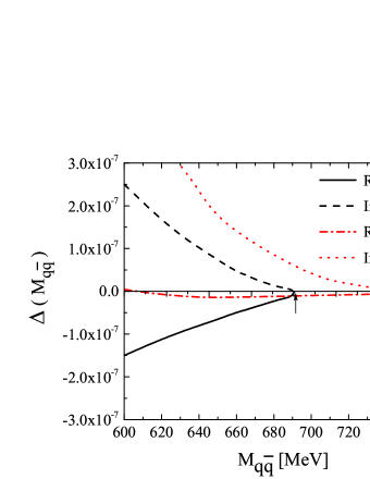
Figure 5: An illustration of the approach of the pole mass solution to the thermal mass $2\pi T$ at large temperatures for the Matsubara frequency with $N=1$. The real and imaginary parts of the determinant $\Delta$ at $T=110$ MeV are depicted by solid and dashed curves, respectively. The real and imaginary parts at $T=120$ MeV correspond to dotted and dot-dashed lines. The arrows point to the limit $|\bf P|=0$, i.e. the thermal mass limit.

We investigate now also the influence the Debye mass on the bound states for $N=1$. For this we consider the tBS equation with the solution of tDS equation with Debye mass taken into account. Results are exhibited in Fig. 6, where the solid curve denotes the pole mass without the Debye mass, cf. Fig. 4, and the dashed curve illustrates the effect of the Debye mass. As expected, at low temperatures, where $m_{g}$ is small, the two solutions are practically the same. At intermediate values of $T$, the interaction kernel is more compact, hence it leads to larger values of the masses. At larger temperatures both solutions approach the thermal mass limit, see Fig. 5. For completeness, in Fig. 6 we also present the values of two quasi-free quark masses $M_{2q}\equiv 2B({\bf 0},\omega_{0})/A({\bf 0},\omega_{0})$, as solutions of tDS equation with Debye mass (dot-dashed curve) and without Debye mass (dotted curve). It is seen that with Debye mass taken into account the pole mass becomes larger than the two free masses at already $T\sim 90$ MeV, i.e. the dissociation occurs at lower temperatures. This is in agreement with the behaviour of the inflection points $\chi_{B}$ of the mass solution $B$ and $\chi_{q\bar{q}}$ of the quark condensate $\langle q\bar{q}\rangle$, cf. Fig. 3.

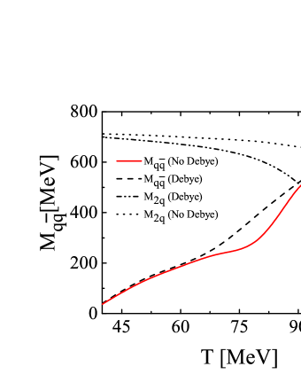
Figure 6: Comparison of the tBS solution for the Matsubara frequency with $N=1$ with (dashed curve) and without (solid curve) taking into account the Debye mass in the tDS equation. The dash-dotted and dotted curves represent the sum of masses $M_{q}\equiv B({\bf 0},\omega_{0})/A({\bf 0},\omega_{0})$ of two free quarks obtained from the solution of the tDS equation, also with and without the Debye mass, respectively.

VII Summary

We have investigated the solution of the truncated Dyson-Schwinger (tDS) equation at finite temperature within the rainbow approximation by employing the Alkofer-Watson-Weigel (AWW) model which consists only of the infra-red term in a more complex interaction kernel. The solution of the tDS equation is a prerequisite for a consistent solution of the truncated Bethe-Salpeter (tBS) equation for quark-antiquark bound states at finite temperature within the same approximation. The ultimate goal is to use the tBS equations, for an analysis of the behaviour of hadrons in hot matter, including possible (phase) transitions and dissociation effects. For this goal we investigate to what extent the model, which provides a fairly good description of ground-state mesons at zero temperatures, can be applied to the truncated tDS equation at finite temperatures. We find that a direct inclusion of the Debye mass in the interaction kernel results in a too low value of the pseudo-critical temperature $T_{c}$, defined as the inflection point of the mass function $B({\bf 0},\omega_{0})$ or/and of the normalized quark condensate $\langle q\bar{q}\rangle$, being by ${\cal O}(50\%)$ smaller than the ones found in lattice QCD calculations. Since in the considered model at a given temperature $T$, the Debye mass $m_{g}$ enters into the longitudinal part of the interaction as a (constant) Gaussian exponential factor $\propto\exp(-16\pi^{2}T^{2}/5\omega^{2})$, it makes problematic the attempts of obtaining larger values of the QCD deconfinement temperature $T_{c}$ close to the lattice values. We argue that, since the Debye mass $m_{g}$ is essentially a perturbative quantity, it has to be taken into account in the perturbative ultra-violet term to maintain a correct behaviour at large momenta, while in the nonperturbative infra-red term it can be omitted at all. We find that by omitting the Debye mass $m_{g}$ one is able to obtain critical temperatures closer (smaller by only 10-15%) to that from lattice $2+1$ flavour QCD. To achieve a better agreement with lattice data the IR term requires further meticulous analyse of the tDS equation at finite temperatures which will be done elsewhere.

As in the case of zero temperature, $T=0$, we consider the tBS equation within the rainbow approximation with the quark propagators entering the tBS equation found preliminarily as solutions of the tDS equation at the same temperature. In our calculations, we restrict the boson Matsubara frequency $\Omega_{N}=2\pi NT$ to $N=1$ and $N=2$. Larger values of $N$ provide large values of $M_{q\bar{q}}$ ($N>2$), far above masses of known lightest pseudo-scalar mesons. For each Matsubara frequency $\Omega_{N}$, the ground state mass $M_{q\bar{q}}^{2}=4\pi^{2}N^{2}T^{2}-{\bf P}^{2}$ is defined as the first (lowest) zero of the corresponding determinant as a function of $|{\bf P}|$. Such a mass is referred to as the Matsubara pole mass.

For both frequencies $\Omega_{N}$, $N=1$ and $N=2$, we find that the pole masses rapidly increase with increase of temperature. This is in agreement with the behaviour of the screening masses at large temperatures reported in literature, see e.g. Refs. yaponetz ; kalinovsky . It has been found that, for the lowest Matsubara frequency, where $N=1$, a solution of the tBS equation at large temperatures, $T>110$ MeV, can be found only in the limit of thermal masses, i.e. at $|{\bf P}|\to 0$. We analyse the behaviour of the pole masses as a function of temperature with respect to the $T$ dependence of the masses of free quarks obtained from the tDS equation. At large values of $T$, $T>100$ MeV, the pole masses become larger than the sum of two quarks. This implies that at large $T$ the ground state of two quark does not occur in the sense as commonly adopted in quantum mechanics where the binding energy is negative. This can be interpreted as dissociation instability of the state against a fragmentation into a state of two quasi-free quarks. The Matsubara pole masses do not have a direct relation to the inertial masses, however, one can expect that the obtained behaviour of the pole masses follow the same tendency as the inertial masses at the same temperature.

References

- (1) C. S. Fischer, S. Kubrak, R. Williams, Spectra of heavy mesons in the Bethe-Salpeter approach, Eur. Phys. J. A51 (2015) 10.
- (2) T. Hilger, M. Gómez-Rocha, A. Krassnigg, Light-quarkonium spectra and orbital-angular-momentum decomposition in a Bethe-Salpeter equation approach, Eur. Phys. J. C77 (2017) 625.
- (3) P. Maris, C. D. Roberts, Pi- and K meson Bethe-Salpeter amplitudes, Phys. Rev. C 56 (1997) 3369.
- (4) P. Maris, P. C. Tandy, Bethe-Salpeter study of vector meson masses and decay constants, Phys. Rev. C 60 (1999) 055214.
- (5) S. M. Dorkin, L. P. Kaptari, B. Kämpfer, Accounting for the analytical properties of the quark propagator from the Dyson-Schwinger equation, Phys. Rev. C 91 (2015) 055201.
- (6) S. M. Dorkin, M. Beyer, S.S. Semikh, L.P. Kaptari, Two-Fermion Bound States within the Bethe-Salpeter Approach, Few Body Syst. 42 (2008) 1.
- (7) T. Hilger, C. Popovici, M. Gomez-Rocha, A. Krassnigg, Spectra of heavy quarkonia in a Bethe-Salpeter-equation approach, Phys. Rev. D 91 (2015) 034013.
- (8) P. Maris, C. D. Roberts, Dyson-Schwinger equations: A tool for hadron physics, Int. J. Mod. Phys. E 12 (2003) 297.
- (9) A. Holl, A. Krassnigg, C. D. Roberts, Pseudoscalar meson radial excitations, Phys. Rev. C 70 (2004) 042203.
-
(10)
M. Blank, A. Krassnigg, Bottomonium in a Bethe-Salpeter-equation study,
Phys. Rev. D 84 (2011) 096014;
M. Blank, A. Krassnigg, A. Maas, Rho-meson, Bethe-Salpeter equation, and the far infrared, Phys. Rev. D 83 (2011) 034020. - (11) D. Jarecke, P. Maris, P. C. Tandy, Strong decays of light vector mesons, Phys. Rev. C 67 (2003) 035202.
- (12) A. Krassnigg, P. Maris, Pseudoscalar and vector mesons as q anti-q bound states, J. Phys. Conf. Ser. 9 (2005) 153.
- (13) C. D. Roberts, M. S. Bhagwat, A. Hol, S. V. Wright, Aspects of hadron physics, Eur. Phys. J. ST 140 (2007) 53.
-
(14)
S. M. Dorkin, T. Hilger, L. P. Kaptari, B. Kämpfer, Heavy pseudoscalar mesons in a Dyson-Schwinger–Bethe-Salpeter approach,
Few Body Syst. 49 (2011) 247;
S. M. Dorkin, L. P. Kaptari, C. Ciofi degli Atti, B. Kämpfer, Solving the Bethe-Salpeter Equation in Euclidean Space, Few Body Syst. 49 (2011) 233. -
(15)
S. -x. Qin, L. Chang, Y. -x. Liu, C. D. Roberts, D. J. Wilson, Interaction model for the gap equation,
Phys. Rev. C 84 (2011) 042202;
S. -x. Qin, L. Chang, Y. -x. Liu, C. D. Roberts, D. J. Wilson, Investigation of rainbow-ladder truncation for excite‘d and exotic mesons, Phys. Rev. C 85 (2012) 035202. - (16) P. Jain, H. J. Munczek, Calculation of the pion decay constant in the framework of the Bethe-Salpeter equation, Phys. Rev. D 44 (1991) 1873.
- (17) H. J. Munczek, P. Jain, Relativistic pseudoscalar q anti-q bound states: Results on Bethe-Salpeter wave functions and decay constants, Phys. Rev D 46 (1992) 438.
- (18) M. R. Frank, C. D. Roberts, Model gluon propagator and pion and rho meson observables Phys. Rev. C 53 (1996) 390.
- (19) R. Alkofer, P. Watson, H. Weigel, Mesons in a Poicare Bethe Salpeter approach, Phys. Rev. D 65 (2002) 094026.
- (20) C. S. Fischer, P. Watson, W. Cassing, Probing unquenching effects in the gluon polarisation in light mesons, Phys. Rev. D 72 (2005) 094025.
- (21) R. Alkofer, L. von Smekal, The Infrared behavior of QCD Green’s functions: Confinement dynamical symmetry breaking, and hadrons as relativistic bound states, Phys. Rept. 353 (2001) 281.
- (22) A. Bender, C. D. Roberts, L. von Smekal, Goldstone theorem and diquark confinement beyond rainbow ladder approximation, Phys. Lett. B 380 (1996) 7.
- (23) R. Delbourgo, M. D. Scadron, Proof of the Nambu-goldstone Realization for Vector Gluon Quark Theories, J. Phys. G: Nucl. Phys. 5 (1979) 1621.
- (24) H. J. Munczek, Dynamical chiral symmetry breaking, Goldstone’s theorem and the consistency of the Schwinger-Dyson and Bethe-Salpeter Equations, Phys. Rev. D 52 (1995) 4736.
- (25) T. Hatsuda,Y. Koike, S. H. Lee, Finite temperature QCD sum rules reexamined: rho, omega and A1 mesons, Nucl. Phys. B394 (1993) 221.
- (26) A. Ayala, A. Bashir, Longitudinal and transverse fermion boson vertex in QED at finite temperature in the HTL approximation, Phys. Rev. D 64 (2001) 025015.
- (27) C. D. Roberts, S. M. Schmidt, Dyson-Schwinger equations: Density, temperature and continuum strong QCD, Prog. Part. Nucl. Phys. 45 (2000) S1-S103.
- (28) T. Matsubara, A New approach to quantum statistical mechanics, Prog. Theor. Phys., 14 (1955) 351.
- (29) R. Haag, N. Hugenholtz, M. Winnink, On the Equilibrium States in Quantum Statistical Mechanics, Commun. Math. Phys. 5 (1967) 215.
- (30) J. Derezinski, C. -A. Pillet, KMS states, pillet.univ-tln.fr/data/pdf/KMS-states.pdf
- (31) J. I. Kapusta, ”Finite-Temperature Field Theory”, Cambridge University Press, N.Y., 1989.
- (32) A. A. Abrikosov, L. P. Gorkov, I. E. Dzyaloshinski, ”Methods of Quantum Field Theory in Statistical Physics”, (editor) R. A. Silverman, PRENTICE-HALL, INC., Englewood Cliffs, New Jersey, 1963.
- (33) C. S. Fischer, J. M. Pawlowski, A. Rothkopf, C. A. Welzbacher, . Bayesian analysis of quark spectral properties from the Dyson-Schwinger equation, e-Print: arXiv: 1705.03207 [hep-ph].
- (34) Kun-lun Wang,Yu-xin Liu, Lei Chang, C. D. Roberts, S .M. Schmidt, Baryon and meson screening masses, Phys.Rev. D 87 (2013) 074038.
- (35) M. Ishii, H. Kouno, M. Yahiro, Model prediction for temp. dep. of meson pole masses from LQCD on meson screening masses, Phys. Rev. D 95 (2017) 114022.
- (36) C. D. Roberts, Hadron Properties and Dyson-Schwinger Equations, Prog. Part. Nucl. Phys. 61 (2008) 50.
- (37) P. D. Morley, M. B. Kislinger, Relativistic Many Body Theory, Quantum Chromodynamics and Neutron Stars/Supernova, Phys. Rept. 51 (1979) 63.
- (38) D. Blaschke, A. Dubinin, A. Radzhabov, A. Wergieluk, Mott dissociation of pions and kaons in hot, dense quark matter, Phys.Rev. D96 (2017) 094008.
- (39) J. M. Pawlowski, N. Strodthoff, N. Wink, Finite temperature spectral functions in the O(N)-model, E-print: arXiv 1711.07444 [hep-th].
- (40) N. Strodthoff, Self-consistent spectral functions in the O(N) model from the functional renormalization group, Phys. Rev. D95 (2017) 076002.
- (41) J.M. Pawlowski, N. Strodthoff, Real time correlation functions and the functional renormalization group, Phys. Rev. D92 (2015) 094009.
- (42) P. Maris, C. D. Roberts, QCD modeling of hadron physics, Nucl. Phys. Proc. Suppl. 161 (2006) 136-152.
- (43) C. D. Roberts, A. Williams, Dyson-Schwinger equations and their application to hadronic physics, Prog. Part. Nucl. Phys. 33 (1994) 477.
- (44) S-X Qin, L. Chang, Y-X Liu, C. D. Roberts, Quark spectral density and a strongly-coupled QGP, Phys. Rev. D 84 (2011) 014017.
- (45) P. Maris, C. D. Roberts, S. M. Schmidt, P. C. Tandy, T - dependence of pseudoscalar and scalar correlations, Phys. Rev. C 63 (2001) 025202.
- (46) Si-xue Qin, Dirk H. Rischke, Quark Spectral Function and Deconfinement at Nonzero Temperature, Phys. Rev. D88 (2013) 056007.
- (47) S. M.Dorkin, M. Viebach, L. P. Kaptari, B. Kämpfer, Extending the truncated Dyson-Schwinger equation to finite temperatures, J. Mod.Phys. 7 (2016) 2071; e-Print: arXiv:1512.06596 [nucl-th].
- (48) M. Blank, A. Krassnigg, The QCD chiral transition temperature in a Dyson-Schwinger-equation context, Phys. Rev. D 82 (2010) 034006.
-
(49)
Fei Gao, Jing Chen, Yu-Xin Liu, Si-Xue Qin, Craig D. Roberts, Sebastian M. Schmidt,
Phase diagram and thermal properties of strong-interaction matter,
Phys. Rev. D 93 (2016), 094019;
F. Gao, S.-X. Qin, Y.-X. Liu, C. D. Roberts, S. M. Schmidt, Zero mode in a strongly coupled quark gluon plasma, Phys. Rev. D 89 (2014) 076009. - (50) F. Karsch, M. Kitazawa, Quark propagator at finite temperature and finite momentum in quenched lattice QCD, Phys. Rev. D 80 (2009) 056001.
- (51) C. S. Fischer, J. Luecker, C. A. Welzbacher, Phase structure of three and four flavor QCD, Phys. Rev. D 90 (2014) 034022.
- (52) C. S. Fischer, J. A. Mueller, Chiral and deconfinement transition from Dyson-Schwinger equations, Phys. Rev. D 80 (2009) 074029.
-
(53)
G. Eichmann, C. S. Fischer, C. A. Welzbacher,
Baryon effects on the location of QCD’s critical end point,
Phys. Rev. D 93 (2016) 034013;
C. S. Fischer, J. Lueckerb, C. A. Welzbacher, Locating the critical end point of QCD, Nucl. Phys. A 931 (2014) 774. - (54) Hui-Feng Fu, Qing Wang, Quark propagator in a truncation scheme beyond the rainbow approximation, Phys. Rev. D 93 (2016) 014013.
- (55) D. Binosi, Lei Chang, J. Papavassiliou, Si-Xue Qin, C. D. Roberts, Symmetry preserving truncations of the gap and Bethe-Salpeter equations, Phys. Rev. D 93 (2016) 096010.
- (56) B. El-Bennich, G. Krein, E Rojas, F E. Serna, Excited hadrons and the analytical structure of bound-state interaction kernels Few Body Syst. 57 (2016) 955.
- (57) Y. Aoki, S. Borsanyi, S. Durr, Z. Fodor, S. D. Katz, S. Krieg, K. K. Szabo, The QCD transition temperature: results with physical masses in the continuum limit II, JHEP 0906 (2009) 88.
- (58) C. S. Fischer, A. Maas, J. M. Pawlowski, On the infrared behavior of Landau gauge Yang-Mills theory, Ann. Phys. 324 (2009) 2408.
- (59) M. R. Pennington, D. J. Wilson, Are the Dressed Gluon and Ghost Propagators in the Landau Gauge presently determined in the confinement regime of QCD?, Phys. Rev. D 84 (2011) 094028; [ibid. D 84 (2011) 119901, Erratum].
- (60) N. Souchlas, Infrared and Ultraviolet QCD dynamics with quark mass for J=0,1 mesons, arXiv:nucl-th/1006.0942, June 2010.
- (61) H. Umezawa, H. Matsumoto, M. Tachiki, ”Termo Field Dynamics and Condensed States” (North-Holland, Amsterdam, 1982).
- (62) A. J. Niemi, G. W. Semenoff, Finite Temperature Quantum Field Theory in Minkowski Space, Ann. Phys. 152 (1984) 105.
- (63) Michel le Bellac, ”Thermal Filed Theory”, Cambridge Monographs on Mathematical Physics, General Editors: P. V. Landshoff, D. R. Nelson, D. W. Sciama, S. Weinberg, Cambridge University Press 1996 .
- (64) P. C. Martin, J. Schwinger, Theory of many particle systems. 1. Phys. Rev., 115 (1959) 1342.
- (65) N. P. Landsman, Ch. G. van Weert, Real and Imaginary Time Field Theory at Finite Temperature and Density, Phys. Rept. 145 (1987) 141.
- (66) A. Cucchieri, A. Maas, T. Mendes, Infrared properties of propagators in Landau-gauge pure Yang-Mills theory at finite temperature, Phys. Rev. D 75 (2007) 076003.
- (67) M. Harada, S. Tagaki, Phase transition in two flavor dense QCD from the Schwinger-Dyson equation, Prog. Theor. Phys. 107 (2002) 561.
- (68) D. K. Hong, V. A. Miransky, I. A. Shovkovy, L. C. R. Wijewardhana, Schwinger-Dyson approach to color superconductivity in dense QCD, Phys. Rev. D61 (2000), 056001, [ibid. D 62, (2000),059903, Erratum].
- (69) R. Alkofer, P. A. Amundsen, K. Langfeld, Chiral Symmetry Breaking and Pion Properties at Finite Temperatures, Z. Phys. C 42 (1989) 199.
- (70) S. Tagaki, Phase structure of hot and / or dense QCD with the Schwinger-Dyson equation, Prog. Theor. Phys. 109 (2003) 233.
- (71) D. Blaschke, G. Burau, Yu. L. Kalinovsky, P. Maris, P. C. Tandy, Finite T meson correlations and quark deconfinement, Int. J . Mod. Phys.A16 (2001) 2267-2291 A. Bender, D. Blaschke, Yu. Kalinovsky, C. D. Roberts, Continuum study of deconfinement at finite temperature, Phys. Rev. Lett. 77 (1996) 3724.
- (72) S. M. Dorkin, L. P. Kaptari, T. Hilger, B. Kämpfer, Analytical properties of the quark propagator from a truncated Dyson-Schwinger equation in complex Euclidean space, Phys. Rev. C 89 (2014) 034005.
- (73) S. Llewellyn, A relativistic formulation for the quark model for mesons, Ann. of Phys. 53 (1969) 521.
- (74) C. S. Fischer, J. Luecker, Propagators and phase structure of Nf=2 and Nf=2+1 QCD, Phys. Lett. B 718 (2013) 1036.
-
(75)
S. Fritzsche,
Maple procedures for the coupling of angular momenta. An up-date of the Racah module,
Computer Physics Communication 180 (2009) 2021;
Program summary URL:
http://cpc.cs.qub.ac.uk/summaries/ADFV_v10_0.html